arX

iv:a

stro

-ph/

0512

030v

1 1

Dec

200

5

A Parallel Adaptive P3M code with

Hierarchical Particle Reordering

Robert J. Thacker a,1 and H. M. P. Couchman b

aDepartment of Physics, Engineering Physics and Astronomy, Queen’s University,

Kingston, Ontario, K7L 3N6

bDepartment of Physics and Astronomy, McMaster University, 1280 Main St.

West, Hamilton, Ontario, L8S 4M1, Canada.

Abstract

We discuss the design and implementation of HYDRA OMP a parallel implemen-tation of the Smoothed Particle Hydrodynamics–Adaptive P3M (SPH-AP3M) codeHYDRA. The code is designed primarily for conducting cosmological hydrodynamicsimulations and is written in Fortran77+OpenMP. A number of optimizations forRISC processors and SMP-NUMA architectures have been implemented, the mostimportant optimization being hierarchical reordering of particles within chainingcells, which greatly improves data locality thereby removing the cache misses typi-cally associated with linked lists. Parallel scaling is good, with a minimum parallelscaling of 73% achieved on 32 nodes for a variety of modern SMP architectures. Wegive performance data in terms of the number of particle updates per second, whichis a more useful performance metric than raw MFlops. A basic version of the codewill be made available to the community in the near future.

Key words: Simulation, cosmology, hydrodynamics, gravitation, structureformation

PACS: 02:60.-x 95:30.Sf 95:30.Lz 98:80.-k

1 Introduction

The growth of cosmological structure in the Universe is determined primar-ily by (Newtonian) gravitational forces. Unlike the electrostatic force, whichcan be both attractive and repulsive and for which shielding is important, the

1 CITA National Fellow

Preprint submitted to Elsevier Science 4 June 2018

ubiquitous attraction of the gravitational force leads to extremely dense struc-tures, relative to the average density in the Universe. Galaxies, for example, aretypically 104 times more dense than their surrounding environment, and sub-structure within them can be orders of magnitude more dense. Modelling suchlarge density contrasts is difficult with fixed grid methods and, consequently,particle-based solvers are an indispensable tool for conducting simulations ofthe growth of cosmological structure. The Lagrangian nature of particle codesmakes them inherently adaptive without requiring the complexity associatedwith adaptive Eulerian methods. The Lagrangian Smoothed Particle Hydro-dynamics (SPH,(1)) method also integrates well with gravitational solversusing particles, and because of its simplicity, robustness and ability to easilymodel complex geometries, has become widely used in cosmology. Further,the necessity to model systems in which orbit crossing, or phase wrapping,occurs (either in collisionless fluids or in collisional systems) demands a fullyLagrangian method that tracks mass. While full six-dimensional (Boltzmann)phase-space models have been attempted, the resolution is still severely limitedon current computers for most applications.

Particle solvers of interest in cosmology can broadly be divided into hybriddirect plus grid-based solvers such as Particle-Particle, Particle-Mesh meth-ods (P3M,(2)) and “Tree” methods which use truncated low order multipoleexpansions to evaluate the force from distant particles (3). Full multipolemethods (4), are slowly gaining popularity but have yet to gain widespreadacceptance in the cosmological simulation community. There are also a num-ber of hybrid tree plus particle-mesh methods in which an efficient grid-basedsolver is used for long-range gravitational interactions with sub-grid forcesbeing computed using a tree. Special purpose hardware (5) has rendered thedirect PP method competitive in small simulations (fewer than 16 millionparticles), but it remains unlikely that it will ever be competitive for largersimulations.

The P3M algorithm has been utilized extensively in cosmology. The first highresolution simulations of structure formation were conducted by Efstathiou& Eastwood (6) using a modified P3M plasma code. In 1998 the Virgo Con-sortium used a P3M code to conduct the first billion particle simulation ofcosmological structure formation (7). The well-known problem of slow-downunder heavy particle clustering, due to a rapid rise in the number of short-range interactions, can be largely solved by the use of adaptive, hierarchical,sub-grids (8). Only when a regime is approached where multiple time stepsare beneficial does the adaptive P3M (AP3M) algorithm become less compet-itive than modern tree-based solvers. Further, we note that a straightforwardmultiple time-step scheme has been implemented in AP3M with a factor of 3speed-up reported (9).

P3M has also been vectorized by a number of groups including Summers (10).

2

Shortly after, both Ferrell & Bertschinger (11) and Theuns (12) adapted P3Mto the massively parallel architecture of the Connection Machine. This earlywork highlighted the need for careful examination of the parallelization strat-egy because of the load imbalance that can result in gravitational simula-tions as particle clustering develops. Parallel versions of P3M that use a 1-dimensional domain decomposition, such as the P4M code of Brieu & Evrard(13) develop large load imbalances under clustering rendering them usefulonly for very homogeneous simulations. Development of vectorized treecodes(14; 15) predates the early work on P3M codes and a discussion of a com-bined TREE+SPH (TREESPH) code for massively parallel architectures ispresented by Dave et al. (16). There are now a number of combined parallelTREE+SPH solvers (17; 18; 19; 20) and TREE gravity solvers (21; 22; 45).Pearce & Couchman (23) have discussed the parallelization of AP3M+SPH onthe Cray T3D using Cray Adaptive Fortran (CRAFT), which is a directive-based parallel programming methodology. This code was developed from theserial HYDRA algorithm (25) and much of our discussion in this paper drawsfrom this first parallelization of AP3M+SPH. A highly efficient distributedmemory parallel implementation of P3M using the Cray SHMEM library hasbeen developed by MacFarland et al. (26), and further developments of thiscode include a translation to MPI-2, the addition of AP3M subroutines and theinclusion of an SPH solver (24). Treecodes have also been combined with gridmethods to form the Tree-Particle-Mesh solver (27; 28; 30; 29; 31; 32). The al-gorithm is somewhat less efficient than AP3M in a fixed time-step regime, butits simplicity offers advantages when multiple time-steps are considered (32).Another interesting, and highly efficient N-body algorithm is the Adaptive Re-finement Tree (ART) method (33) which uses a short-range force correctionthat is calculated via a multi-grid solver on refined meshes.

There are a number of factors in cosmology that drive researchers towardsparallel computing. These factors can be divided into the desire to simulatewith the highest possible resolution, and hence particle number, and also theneed to complete simulations in the shortest possible time frame to enablerapid progress. The desire for high resolution comes from two areas. Firstly,simultaneously simulating the growth of structure on the largest and small-est cosmological scales requires enormous mass resolution (the ratio of massscales between a supercluster and the substructure in a galaxy is > 109). Thisproblem is fundamentally related to the fact that in the currently favouredCold Dark Matter (34) cosmology structure grows in a hierarchical manner.A secondary desire for high resolution comes from simulations that are per-formed to make statistical predictions. To ensure the lowest possible samplevariance the largest possible simulation volume is desired.

For complex codes, typically containing tens of thousands of lines, the effortin developing a code for distributed-memory machines, using an API such asMPI (35), can be enormous. The complexity within such codes arises from the

3

subtle communication patterns that are disguised in serial implementations.Indeed, as has been observed by the authors, development of an efficient com-munication strategy for a distributed memory version of the P3M code hasrequired substantially more code than the P3M algorithm itself (see (26)).This is primarily because hybrid, or multi-part solvers, of which P3M is aclassic example, have data structures that require significantly different datatopologies for optimal load balance at different stages of the solution cycle.Clearly a globally addressable work space renders parallelization a far simplertask in such situations. It is also worth noting that due to time-step constraintsand the scaling of the algorithm with the number of particles, doubling the lin-ear resolution along an axis of a simulation increases the computational workload by a factor larger than 20; further doubling would lead to a workload inexcess of 400 times greater.

The above considerations lead to the following observation: modern SMPservers with their shared memory design and superb performance character-istics are an excellent tool for conducting simulations requiring significantlymore computational power than that available from a workstation. Althoughsuch servers can never compete with massively parallel machines for the largestsimulations, their ease of use and programming renders them highly produc-tive computing environments. The OpenMP (http://www.openmp.org) APIfor shared-memory programming is simple to use and enables loop level par-allelism by the insertion of pragmas within the source code. Other than theirlimited expansion capacity, the strongest argument against purchasing an SMPserver remains hardware cost. However, there is a trade-off between scienceaccomplishment and development time that must be considered above hard-ware costs alone. Typically, programming a Beowulf-style cluster for challeng-ing codes takes far longer and requires a significantly greater monetary andpersonnel investment on a project-by-project basis. Conversely, for problemsthat can be efficiently and quickly parallelized on a distributed memory ar-chitecture, SMP servers are not cost effective. The bottom line remains thatindividual research groups must decide which platform is most appropriate.

The code that we discuss in this paper neatly fills the niche between work-station computations and massively parallel simulations. There is also a classof simulation problems in cosmology that have particularly poor parallel scal-ing, regardless of the simulation algorithm used (the fiducial example is themodelling of single galaxies, see (53)). This class of problems corresponds toparticularly inhomogeneous particle distributions that develop a large dispar-ity in particle-update timescales (some particles may be in extremely denseregions, while others may be in very low density regions). Only a very smallnumber of particles—insufficient to be distributed effectively across multiplenodes—will require a large number of updates due to their small time-steps.For this type of simulation the practical limit of scalability appears to be order10 PEs.

4

The layout of the paper is as follows: in section 2 we review the physicalsystem being studied. This is followed by an extensive exposition of the P3Malgorithm and the improvements that yield the AP3M algorithm. The primarypurpose of this section is to discuss some subtleties that directly impact ourparallelization strategy. At the same time we also discuss the SPH methodand highlight the similarities between the two algorithms. Section 2 concludeswith a discussion of the serial HYDRA code. Section 3 begins with a shortdiscussion of the memory hierarchy in RISC (Reduced Instruction Set Com-puter) systems, and how eliminating cache-misses and ensuring good cachereuse ensures optimal performance on these machines. This is followed by adiscussion of a number of code optimizations for RISC CPUs that also leadto performance improvements on shared memory parallel machines (primarilydue to increased data locality). In particular we discuss improvements in par-ticle bookkeeping, such as particle index reordering. While particle reorderingmight be considered an expensive operation, since it involves a global sort, itactually dramatically improves run time because of bottlenecks in the memoryhierarchy of RISC systems. In section 4 we discuss in detail the parallelizationstrategies adopted in HYDRA OMP. To help provide further understandingwe compare the serial and parallel call trees. In section 5 we consolidate ma-terial from sections 3 & 4 by discussing considerations for NUMA machinesand in particular the issue of data placement. Performance figures are givenin Section 6, and we present our conclusions in section 7.

2 Review of the serial algorithm

2.1 Equation set to be solved

The simulation of cosmic structure formation is posed as an initial value prob-lem. Given a set of initial conditions, which are usually constrained by ex-perimental data, such as the WMAP data (37), we must solve the followinggravito-hydrodynamic equations;

(1) the continuity equations,

dρgdt

+ ρg∇.vg = 0,dρdmdt

+ ρdm∇.vdm = 0 (1)

where g denotes gas and dm dark matter.(2) the Euler and acceleration equations,

dvg

dt= −

1

ρg∇P −∇φ,

dvdm

dt= −∇φ, (2)

5

(3) the Poisson equation,

∇2φ = 4πG(ρg + ρdm), (3)

(4) the entropy conservation equation,

ds

dt= 0, (4)

where the conservation of entropy is a result of ignoring dissipation, viscosityand thermal conductivity (i.e. an ideal fluid). The dynamical system is closedby the equation of state P = P (ρg, s). We assume an ideal gas equation ofstate, with γ = 5/3 in our code, although many others are possible. Alterna-tively, the entropy equation can be substituted with the conservation of energyequation,

du

dt= −

P

ρg∇.vg, (5)

and the equation of state is then P = P (ρg, u). We note that the use of aparticle-based method ensures that the continuity equations are immediatelysatisfied.

2.2 Gravitational solver

Let us first discuss the basic features of the P3M algorithm, a thorough reviewcan be found in (2). The fundamental basis of the P3M algorithm is that thegravitational force can be separated into short and long range components,i.e. ,

Fgrav = Fshort + Flong, (6)

where Flong will be provided by a Fourier-based solver and Fshort will becalculated by summing over particles within a given short range radius. TheFlong force is typical known as the PM force, for Particle-Mesh, while theFshort range force is typical known as the PP force, for Particle-Particle. Theaccuracy of the Fgrav force can be improved by further smoothing the meshforce, Flong, and hence increasing the range over the which the short-scalecalculation is done, at the cost of an increased number of particle–particleinteractions.

The first step in evaluating that PM force is to interpolate the mass densityof the particle distribution on to a grid which can be viewed as a map froma Lagrangian representation to an Eulerian one. The interpolation function

6

we use is the the ‘Triangular Shaped Cloud’ (TSC) ‘assignment function’ (see(2) for a detailed discussion of possible assignment functions). Two benefitsof using TSC are good suppression of aliasing from power above the Nyquistfrequency of the grid and a comparatively low directional force error aroundthe grid spacing. The mass assignment operation count is O(N), where N isthe number of particles.

Once the mass density grid has been constructed it is Fourier transformed us-ing an FFT routine, which is anO(L3 logL) operation, where L is the extent ofthe Fourier grid in one direction. The resulting k-space field is then multipliedwith a Green’s function that is calculated to minimize errors associated withthe mass assignment procedure (see Hockney & Eastwood for a review of the‘Q-minimization’ procedure). Following this convolution, the resulting poten-tial grid is differenced to recover the force grid. We use a 10-point differencingoperator which incorporates off-axis components and reduces directional forceerrors, but many others are possible. Finally, the PM accelerations are foundfrom the force grid using the mass assignment function to interpolate the ac-celeration field. The PM algorithm has an operation cost that is approximatelyO(αN + βL3 logL) where α and β are constants (the O(L3) cost of the dif-ferencing is adequately approximated by the logarithmic term describing theFFT) .

Resolution above the Nyquist frequency of the PM code, or equivalently subPM grid resolution, is provided by the pair-wise (shaped) short-range forcesummation. Supplementing the PM force with the short-range PP force givesthe full P3M algorithm, and the execution time scales approximately in pro-portion to αN+βL3 log L + γ

∑

N2

pp, where γ is a constant and N2

pp correspondsto the number of particles in the short range force calculation within a spec-ified region. The summation is performed over all the PP regions, which areidentified using a chaining mesh of size Ls3; see figure 1 for an illustrationof the chaining mesh overlaid on the potential mesh. P3M suffers the draw-back that under heavy gravitational clustering the short range sum used tosupplement the PM force slows the calculation down dramatically - the N2

pp

term dominates as an increasingly large number of particles contribute to theshort range sum. Although acutely dependent upon the particle number andrelative clustering in a simulation, the algorithm may slow down by a factorbetween 10-100 or possibly more. While finer meshes partially alleviate thisproblem they quickly become inefficient due to wasting computation on areasthat do not need higher resolution.

Adaptive P3M remedies the slow-down under clustering of P3M by isolatingregions where the N2

pp term dominates and solving for the short range force inthese regions using FFT methods on a sub-grid, which is then supplementedby short range calculations involving fewer neighbours. This process is a re-peat of the P3M algorithm on the selected regions, with an isolated FFT and

7

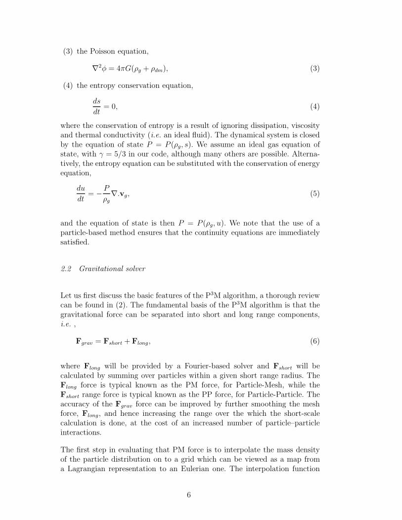
Particle chaining mesh

Neighboursearch radius

PotentialMesh

Fig. 1. Overlay of the chaining mesh on top of the potential mesh to show spacingand the search radius of the short range force. These two meshes do not need tobe commensurate except on the scale of the box, the required matching of forces isachieved by shaping the long and short range force components, Fshort and Flong.

shaped force. At the expense of a little additional bookkeeping, this methodcircumvents the sometimes dramatic slow-down of P3M. The operation countis now approximately,

αN + βL3 logL+nref∑

j=1

[

αjNj + βjL3

j logL+ γj∑

N2

jpp

]

, (7)

where nref is the number of refinements. The αj and γj are all expected to bevery similar to the α, and γ of the main solver, while the βj are approximatelyfour times larger than β due to the isolated Fourier transform. Ideally duringthe course of the simulation the time per iteration approaches a constant,roughly 2-4 times that of a uniform distribution (although when the SPHalgorithm is included this slow-down can be larger).

2.3 SPH solver

When implemented in an adaptive form (38), with smoothing performed overa fixed number of neighbour particles, SPH is an order N scheme and fits

8

well within the P3M method since the short-range force-supplement for themesh force can be used to find the particles which are required for the SPHcalculation. There are a number of excellent reviews of the SPH methodology(15; 39; 40) and we present, here, only those details necessary to understandour specific algorithm implementation. Full details of our implementation canbe found in (41).

We use an explicit ‘gather’ smoothing kernel and the symmetrization of theequation of motion is achieved by making the replacement,

∇jW (ri − rj, hj , hi) = −∇iW (ri − rj, hi, hj) +O(∇h) (8)

in the ‘standard’ SPH equation of motion (see (40), for example). Note thatthe sole purpose of ‘kernel averaging’ in this implementation, denoted by thebar on the smoothing kernel W , is to ensure that the above replacement iscorrect to O(h). Hence the equation of motion is,

dvi

dt= −

N∑

j=1,rij<2hi

mj (Pi

ρ2i+

Πij

2) ∇iW (ri − rj, hi, hj)

+N∑

j=1,rij<2hj

mj (Pj

ρ2j+

Πji

2) ∇jW (ri − rj, hj, hi). (9)

The artificial viscosity, Πij, is used to prevent interpenetration of particle flowsand is given by,

Πij =−αµij cij + βµ2

ij

ρijfi, (10)

where,

µij =

hijvij.rij/(r2

ij + ν2), vij.rij < 0;0, vij.rij ≥ 0,

(11)

ρij = ρi(1 + (hi/hj)3)/2, (12)

and

fi =|< ∇.v >i|

|< ∇.v >i|+ |< ∇×v >i|+ 0.0001ci/hi

. (13)

with bars being used to indicate averages over the i, j indices. Shear-correction(42; 43), is achieved by including the fi term which reduces the—unwanted—

9

artificial viscosity in shearing flows. Note that the lack of i − j symmetry inΠij is not a concern since the equation of motion enforces force symmetry.

The energy equation is given by,

dui

dt=

N∑

j=1,rij<2hi

mj(Pi

ρ2i+

Πij

2) (vi − vj).∇iW (ri − rj, hi, hj). (14)

The solution of these equations is comparatively straightforward. As in theAP3M solver it is necessary to establish the neighbour particle lists. The den-sity of each particle must be evaluated and then, in a second loop, the solutionto the force and energy equations can be found. Since the equation of motiondoes not explicitly depend on the density of particle j (the artificial viscosityhas also been constructed to avoid this) we emphasize that there is no needto calculate all the density values first and then calculate the force and en-ergy equations. If one does calculate all densities first, then clearly the listof neighbours is calculated twice, or alternatively, a large amount of memorymust be used to store the neighbour lists of all particles. Using our method thedensity can be calculated, one list of neighbours stored, and then the force andenergy calculations can be quickly solved using the stored list of neighbours(see (25)).

2.4 Summary of solution cycle for each iteration

As emphasized, the list data-structure used in the short-range force calculationprovides a common feature between the AP3M and SPH solvers. Hence, once alist of particle neighbours has been found, it is simple to sort through this andestablish which particles are to be considered for the gravitational calculationand the SPH calculation. Thus the incorporation of SPH into AP3M necessi-tates only the coordination of scalings and minor bookkeeping. The combinedadaptive P3M-SPH code, ‘HYDRA’, in serial FORTRAN 77 form is availableon the World Wide Web from http://coho.physics.mcmaster.ca/hydra.

The solution cycle of one time-step may be summarized as follows,

(1) Assign mass to the Fourier mesh.(2) Convolve with the Green’s function using the FFT method to get poten-

tial. Difference this to recover mesh forces in each dimension.(3) Apply mesh force and accelerate particles.(4) Decide where it is more computationally efficient to solve via the further

use of Fourier methods as opposed to short-range forces and, if so, placea new sub-mesh (refinement) there.

10

(5) Accumulate the gas forces (and state changes) as well as the short rangegravity for all positions not in sub-meshes.

(6) Repeat 1-5 on all sub-meshes until forces on all particles in simulationhave been accumulated.

(7) Update time-step and repeat

Note that the procedure of placing meshes is hierarchical in that a furthersub-mesh may be placed inside a sub-mesh. This procedure can continue toan arbitrary depth but, typically, even for the most clustered simulations,speed-up only occurs to a depth of six levels of refinement.

A pseudo call-tree for the serial algorithm can be seen in figure 2. The purposeof each subroutine is as follows,

• STARTUP Reads in data and parameter files• INUNIT Calculates units of simulation from parameters in start-up files• UPDATERV Time-stepping control• OUTPUT Check-pointing and scheduled data output routines• ACCEL Selection of time-step criteria and corrections, if necessary, for co-moving versus physical coordinates

• FORCE Main control routine of the force evaluation subroutines• RFINIT & LOAD Set up parameters for PM and PP calculation, in LOADdata is also loaded into particle buffers for the refinement.

• CLIST & ULOAD Preparation of particle data for any refinements thatmay have been placed, ULOAD also unloads particle data from refinementbuffers

• REFFORCE Call PM routines, controls particle bookkeeping, call PP rou-tines.

• GREEN & IGREEN Calculation of Green’s functions for periodic (GREEN)and isolated (IGREEN) convolutions.

• MESH & IMESH Mass assignment, convolution call, and calculation of PMacceleration in the periodic (MESH) and isolated (IMESH) solvers.

• CNVLT & ICNVLT Green’s function convolution routines.• FOUR3M 3 dimensional FFT routine for periodic boundary conditions.• LIST Evaluation of chaining cell particle lists• REFINE Check whether refinements need to be placed.• SHFORCE Calculate force look-up tables for PP• SHGRAVSPH Evaluate PP and SPH forces

11

Fig. 2. Call tree of the HYDRA serial algorithm. Only significant subroutines areshown for clarity. The refinement routines are the same as the top level routines,modulo the lack of periodic wrap-around. In an object-oriented framework theseroutines would be prime candidates for overloading.

3 Optimizations of the serial code for RISC processors

3.1 Memory hierarchy of the RISC architecture

The architecture of RISC CPUs incorporates a memory hierarchy with widelydiffering levels of performance. Consequently, the efficiency of a code runningon a RISC processor is dictated almost entirely by the ratio of the time spentin memory accesses to the time spent performing computation. This fact canlead to enormous differences in code performance.

The relative access times for the hierarchy are almost logarithmic. Access tothe first level of cache memory takes 1-2 processor cycles, while access to thesecond level of cache memory takes approximately 5 times as long. Access tomain memory takes approximately 10 times longer. It is interesting to notethat SMP-NUMA servers provide further levels to this hierarchy, as will bediscussed later.

To improve memory performance, when retrieving a word from main memorythree other words are typically retrieved: the ‘cache line’. If the additionalwords are used within the computation on a short time scale, the algorithmexhibits good cache reuse. It is also important to not access memory in dis-ordered fashion, i.e. optimally one should need memory references that arestored within caches. Thus to exhibit good performance on a RISC processor,a code must exhibit both good cache reuse and a low number of cache misses.In practice, keeping cache misses to a minimum is the first objective since

12

cache reuse is comparatively easy to achieve given a sensible ordering of thecalculation (such as a FORTRAN DO loop).

3.2 Serial Optimizations

A number of optimizations for particle codes that run on RISC processors arediscussed in Decyk et al.(45). Almost all of these optimizations are includedwithin our serial code, with the exception of the mass assignment optimiza-tions. Indeed a large number of their optimizations, especially those relating tocombining x, y, z coordinate arrays into one 3-d array, can be viewed as goodprogramming style. While Decyk et al. demonstrate that the complexity of theperiodic mass assignment function prevents compilers from software pipeliningthe mesh writes, we do not include their suggested optimization of removingthe modulo statements and using a larger grid. However, the optimization isnaturally incorporated in our isolated solver.

The first optimization we attempted was the removal of a ‘vectorizeable’ Nu-merical Recipes FFT used within the code (FOURN, see (36)). Although thecode uses an optimized 3-d FFT that can call the FOURN routine repeatedlyusing either 1-d or 2-d FFT strategy (to reduce the number of cache missesexhibited by the FOURN routine when run in 3-d), the overall performanceremains quite poor. Therefore we replaced this routine with the FFTPack (see(48)) routines available from Netlib, and explicitly made the 3-d FFT a com-bination of 1-d FFTs. Although there is no question that FFTW (47) providesthe fastest FFTs on almost all architectures we have found little difference be-tween FFTPack and FFTW within our parallel 3-d FFT routine. The greatestperformance improvement is seen in the isolated solver where the 3-d FFT iscompacted to account for the fact that multiple octants are initially zero.

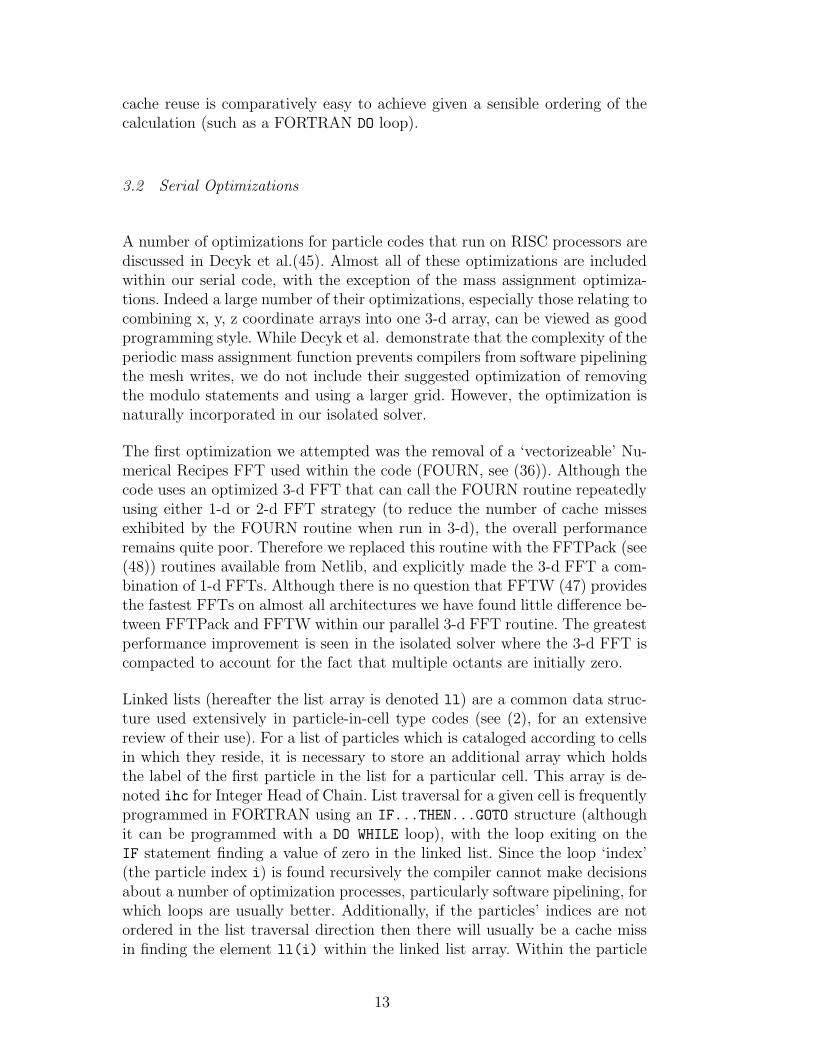
Linked lists (hereafter the list array is denoted ll) are a common data struc-ture used extensively in particle-in-cell type codes (see (2), for an extensivereview of their use). For a list of particles which is cataloged according to cellsin which they reside, it is necessary to store an additional array which holdsthe label of the first particle in the list for a particular cell. This array is de-noted ihc for Integer Head of Chain. List traversal for a given cell is frequentlyprogrammed in FORTRAN using an IF...THEN...GOTO structure (althoughit can be programmed with a DO WHILE loop), with the loop exiting on theIF statement finding a value of zero in the linked list. Since the loop ‘index’(the particle index i) is found recursively the compiler cannot make decisionsabout a number of optimization processes, particularly software pipelining, forwhich loops are usually better. Additionally, if the particles’ indices are notordered in the list traversal direction then there will usually be a cache missin finding the element ll(i) within the linked list array. Within the particle

13

data arrays, the result of the particle indices not being contiguous is anotherseries of cache misses. Since a number of arrays must be accessed to recoverthe particle data, the problem is further compounded, and removal of thecache miss associated with the particle indices should improve performancesignificantly.

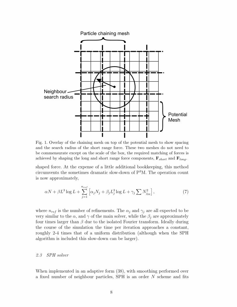
The first step that may be taken to improve the situation is to remove thecache misses associated with the searching through the linked list. To do thisthe list must be formed so that it is ordered. In other words the first particlein cell j, is given by ihc(j), the second particle is given by ll(ihc(j)), thethird by ll(ihc(j)+1) et cetera. This ordered list also allows the short rangeforce calculation to be programmed more elegantly since the IF..THEN..GOTOstructure of the linked list can be replaced by a loop. However, since thereremains no guarantee that the particle indices will be ordered, the compiler isstill heavily constrained in terms of the optimizations it may attempt, but thesituation is distinctly better than for the standard linked list. Tests performedon this ordered list algorithm show that a 30% improvement in speed is gainedover the linked list code (see figure 3). Cache misses in the data arrays are ofcourse still present in this algorithm.

As has been discussed, minimizing cache misses in the particle data arrays re-quires accessing them with a contiguous index. This means that within a givenchaining cell the particle indices must be contiguous. This can be achieved byreordering the indices of particles within chaining cells at each step of theiteration (although if particles need to be tracked a permutation array mustbe carried). This particle reordering idea was realized comparatively early andhas been discussed in the literature (44; 45; 46; 26). A similar concept has beenapplied by Springel (32) who uses Peano-Hilbert ordering of particle indicesto ensure data locality. However, in P3M codes, prior to the implementationpresented here only Macfarland et al.(26) and Anderson and Shumaker (44),actually revised the code to remove linked lists, other codes simply reorderedthe particles every few steps to reduce the probability of cache misses andachieved a performance improvement of up to 45% (26). Since the adaptiverefinements in HYDRA use the same particle indexing method, the particle or-dering must be done within the data loaded into a refinement, i.e. hierarchicalrearrangement of indices results from the use of refinements.

The step-to-step permutation is straightforward to calculate: first the particleindices are sorted according to their z-coordinate and then particle array in-dices are simply changed accordingly. It is important to note that this methodof particle bookkeeping removes the need for an index list of the particles (al-though in practice this storage is taken by the permutation array). All thatneed be stored is the particle index corresponding to the first particle in the celland the number of particles in the cell. On a RISC system particle reordering isso efficient that the speed of the HYDRA simulation algorithm more than dou-

14

0

50

100

150

200

250

300

350

400

0 0.1 0.2 0.3 0.4 0.5 0.6 0.7 0.8 0.9 1 1.1

CPU

tim

e (s

econ

ds)

Cosmological time

Linked listOrdered list (estimate)

Ordered particles

Fig. 3. Effect of changing the list structure on the execution time per iteration ofthe entire algorithm. We show results for the standard linked list implementation,ordered list and ordered particles. The ordered list times were estimated by takingthe ratio between the linked list time and the ordered list time at t=1 and scalingthe rest of the linked list values by this factor. The simulation was the Santa Barbaragalaxy cluster simulation (51) and it was conducted on a 266 Mhz Pentium III PC.

bled. For example, at the end of the Santa Barbara galaxy cluster simulation,the execution time was reduced from 380 seconds to 160 seconds on a 266 MhzPentium III processor. On a more modern 2 Ghz AMD Opteron, which hasfour times the L2 cache of a Pentium III, considerably better prefetch, as wellas an on-die memory controller to reduce latency, we found the performanceimprovement for the final iterations to be a reduction in time from 29 secondsto 17. This corresponds to a speed improvement of a factor of 1.7, which, whileslightly less impressive than the factor of 2.4 seen on the older Pentium III,is still a significant improvement. A comparison plot of the performance of alinked list, ordered list and ordered particle code is shown in figure 3.

4 Parallel Strategy

Particle-grid codes, of the kind used in cosmology, are difficult to parallelizeefficiently. The fundamental limitation to the code is the degree to which theproblem may be subdivided while still averting race conditions and unneces-sary buffering or synchronization. For example, the fundamental limit on thesize of a computational atom in the PP code is effectively a chaining cell,

15

while for the FFT routine it is a plane in the data cube. In practice, loadbalance constraints come into play earlier than theoretical limits as the workwithin the minimal atoms will rarely be equal (and can be orders of magni-tude different). Clearly these considerations set an upper bound on the degreeto which the problem can be subdivided, which in turn limits the number ofprocessors that may be used effectively for a given problem size. The code isa good example of Gustafson’s conjecture: a greater degree of parallelism maynot allow arbitrarily increased execution speed for problems of fixed size, butshould permit larger problems to be addressed in a similar time.

At an abstract level, the code divides into essentially two pieces: the top levelmesh and the refinements. Parallelization of the top level mesh involves paral-lelizing the work in each associated subroutine. Since an individual refinementmay have very little work a parallel scheme that seeks to divide work at allpoints during execution will be highly inefficient. Therefore the following divi-sion of parallelism was made: conduct all refinements of size greater than Nr

particles across the whole machine, for refinements with less than Nr particlesuse a list of all refinements and distribute one refinement to each processor (orthread) in a task farm arrangement. On the T3D the limiting Nr was found tobe approximately 32,768 particles, while on more modern machines we havefound that 262,144 is a better limit.

In the following discussion the term processor element (PE) is used to denotea parallel execution thread. Since only one thread of execution is allottedper processor (we do not attempt load balancing via parallel slackness), thisnumber is equivalent to the number of CPUs, and the two terms are usedinterchangeably. The call tree of the parallel algorithm is given in figure 4.

4.1 The OpenMP standard

The OpenMP API supports a number of parallel constructs, such as exe-cuting multiple serial regions of code in parallel (a single program multi-ple data model), as well as the more typical loop-based parallelism model(sometimes denoted ‘PAR DO’s), where the entire set of loop iterations is dis-tributed across all the PEs. The pragma for executing a loop in parallel, C$OMPPARALLEL DO is placed before the DO loop within the code body. Specificationstatements are necessary to inform the compiler about which variables areloop ‘private’ (each processor carries its own value) and ‘shared’ variables. Afull specification of the details for each loop takes only a few lines of code,preventing the ‘code bloat’ often associated with distributed memory parallelcodes.

16

MAIN

STARTUP INUNIT UPDATERV OUTPUT

ACCEL

FORCE

RFINIT REFFORCE C INDEX

TOP LEVEL(ACROSS THE

WHOLE MACHINE)

LOAD_R REFFORCE_P ULOAD_R

LOAD_P REFFORCE_P ULOAD_P

REFINE SHFORCE SHGRAVSPH_P

CNVLT

FOUR3M

REFINEMENTPLACING ROUTES

GREEN MESH_PLIST_P REORD_P

2 BY 2PSRSSORT

REFINE SHFORCE SHGRAVSPH_P

ICNVLT_P

REFINEMENTPLACING ROUTES

IGREEN IMESH_PLIST_P REORD_P

2 BY 2PSRSSORT

REFINE SHFORCE SHGRAVSPH_R

ICNVLT_R

REFINEMENTPLACING ROUTES

IGREEN IMESH_RLIST_R REORD_R

HPSORT_R

SMALL REFINEMENT(TASK FARM

ACROSS PEs)

LA

RG

E R

EF

INE

ME

NT

(AC

RO

SS

WH

OLE

MA

CH

INE

)

Fig. 4. Call tree of the HYDRA OMP algorithm. Only significant subroutines areshown for clarity. The call tree is similar to the serial algorithm except that anew class of routines is included for large refinements. Where possible conditionalparallelism has been used to enable the reuse of subroutines in serial or parallel.

4.2 Load balancing options provided by the OpenMP standard

We use loop level parallelism throughout our code. To optimize load balance ina given routine it is necessary to select the most optimal iteration schedulingalgorithm. The OpenMP directives allow for the following types of iterationscheduling:

• static scheduling - the iterations are divided into chunks (the size of whichmay be specified if desired) and the chunks are distributed across the pro-cessor space in a contiguous fashion. A cyclic distribution, or a cyclic dis-tribution of small chunks is also available.

• dynamic scheduling - the iterations are again divided up into chunks, how-ever as each processor finishes its allotted chunk, it dynamically obtains thenext set of iterations, via a master-worker mechanism.

• guided scheduling - is similar to static scheduling except that the chunk sizedecreases exponentially as each set of iterations is finished. The minimumnumber of iterations to be allotted to each chunk may be specified.

• runtime scheduling - this option allows the decision on which scheduling touse to be delayed until the program is run. The desired scheduling is thenchosen by setting an environment variable in the operating system.

17

The HYDRA code uses both static and dynamic scheduling.

4.3 Parallelization of particle reordering and permutation array creation

While the step-to-step permutation is in principle simple to calculate, thecreation of the list permutation array must be done carefully to avoid raceconditions. An effective strategy is to calculate the chaining cell residence foreach particle and then sort into bins of like chaining cells. Once particles havebeen binned in this fashion the rearrangement according to z-coordinates is alocal permutation among particles in the chaining cell. Our parallel algorithmworks as follows:

(1) First calculate the chaining cell that each particle resides in, and storethis in an array

(2) Perform an increasing-order global sort over the array of box indices(3) Using a loop over particle indices, find the first particle in each section

of contiguous like-indices (the ihc array)(4) Use this array to establish the number of particles in each contiguous

section (the nhc array)(5) Write the z-coordinates of each particle within the chaining cell into an-

other auxiliary array(6) Sort all the non-overlapping sublists of z-coordinates for all cells in paral-

lel while at the same time permuting an index array to store the preciserearrangement of particle indices required

(7) Pass the newly calculated permutation array to a routine that will rear-range all the particle data into the new order

The global sort is performed using parallel sorting by regular sampling, (49)with a code developed in part by J. Crawford and C. Mobarry. This code hasbeen demonstrated to scale extremely well on shared-memory architecturesprovided the number of elements per CPU exceeds 50,000. This is significantlyless than our ideal particle load per processor (see section 6). For the sortswithin cells, the slow step-to-step evolution of particle positions ensures datarearrangement is sufficiently local for this to be an efficient routine. Hence weexpect good scaling for the sort routines at the level of granularity we typicallyuse.

4.4 Parallelization of mass assignment and Fourier convolution

A race condition may occur in mass assignment because it is possible for PEsto have particles which write to the same elements of the mass array. Theapproaches to solving this problem are numerous but consist mainly of two

18

ideas; (a) selectively assign particles to PEs so that mass assignment occursat grid cells that do not overlap, thus race condition is avoided or (b) useghost cells and contiguous slabs of particles which are constrained in theirextent in the simulation space. The final mass array must be accumulated byadding up all cells, including ghosts. Ghost cells offer the advantage that theyallow the calculation to be load-balanced (the size of a slab may be adjusted)but require more memory. Controlling which particles are assigned does notrequire more memory but may cause a load imbalance. Because the types ofsimulation performed have particle distributions that can vary greatly, bothof these algorithms have been implemented.

4.4.1 Using controlled particle assignment

The particles in the simulation are ordered in the z-direction within the chain-ing cells. Because the chaining cells are themselves ordered along the z-axis(modulo their cubic arrangement) a naive solution would be to simply di-vide up the list of particles. However, this approach does not prevent a racecondition occurring, it merely makes it less likely. In the CRAFT code therace condition was avoided by using the ‘atomic update’ facility which is alock–fetch–update–store–unlock hardware primitive that allows fast updatingof arrays where race conditions are present. Modern cache coherency protocolsare unable to provide this kind of functionality.

Using the linked/ordered list to control the particle assignment provides anelegant solution to the race condition problem. Since the linked list encodesthe position of a particle to within a chaining cell, it is possible to selectivelyassign particles to the mass array that do not have overlapping writes. Toassure a good load balance it is better to use columns (Ls × B × B, whereLs is the size of the chaining mesh and B is a number of chaining cells) ofcells rather than slabs (Ls×Ls×B). Since there are more columns than slabsa finer grained distribution of the computation can be achieved and thus abetter load balance. This idea can also be extended to a 3-d decomposition,however in simple experiments we have found this approach to be inefficientfor all but the most clustered particle distributions (in particular cache reuseis lowered by using a 3-d decomposition).

Chaining mesh cells have a minimum width of 2.2 potential mesh cells in HY-

DRA and figure 1 displays a plot of the chaining mesh overlaid on the potentialmesh. When performing mass assignment for a particle, writes will occur overall 27 grid cells found by the TSC assignment scheme. Thus providing a bufferzone of one cell is not sufficient to avoid the race condition since particles inchaining cells one and three may still write to the same potential mesh cell.A spacing of two chaining mesh cells is sufficient to ensure no possibility ofconcurrent writes to the same mesh cell. The “buffer zones” thus divide up the

19

2x2 blocks whichcan be executedconcurrently

Large arrows indicatethe path through2x2 block groups

Small arrows indicatethe path through2x2 blocks

Fig. 5. Cell grouping and sorting in the 2× 2 configuration scheme.

simulation volume into a number of regions that can calculated concurrentlyand those that cannot. Moreover, there will be need to be a series of barriersynchronizations as regions that can be written concurrently are finished be-fore beginning the next set of regions. The size of the buffer zone means thatthere are two distinct ways of performing the mass assignment using columns:

• Ls× 1× 1 columns in 3× 3 groups. Assign mass for particles in each of thecolumns simultaneously and then perform a barrier synchronization at theend of each column. Since the columns are in 3 × 3 groups there are ninebarriers.

• Ls × 2 × 2 columns which are grouped into 2 × 2 groups. In this case thenumber of barriers is reduced to four, and if desired, the size of the columncan be increased beyond two while still maintaining four barriers. However,load-imbalance under clustering argues against this idea.

See figure 5 for a graphical representation of the algorithm.

To improve load balance, a list of the relative work in each column (that can beevaluated before the barrier synchronization) is calculated by summing overthe number of particles in the column. Once the workload of each column hasbeen evaluated, the list of relative workloads is then sorted in descending order.The calculation then proceeds by dynamically assigning the list of columns tothe PEs as they become free. The only load imbalance then possible is a waitfor the last PE to finish which should be a column with a low workload.Static, and even cyclic, distributions offer the possibility of more severe loadimbalance.

For portability reasons, we have parallelized the FFT by hand rather than

20

relying on a threaded library such as provided by FFTW. The 3-d FFT isparallelized over ‘lines’ by calling a series of 1-d FFTs. We perform the trans-pose operation by explicitly copying contiguous pieces of the main data arrayinto buffers which have a long stride. This improves data locality of the codeconsiderably as the stride has been introduced into the buffer which is a localarray. The FFTs are then performed on the buffer, and values are finally copiedback into the data arrays. The convolution which follows the FFT relies uponanother set of nested loops in the axis directions. To enable maximum gran-ularity we have combined the z- and y-directions into one larger loop whichis then statically decomposed among the processors. Parallel efficiency is highfor this method since if the number of processors divides the size of the FFTgrid we have performed a simple slab decomposition of the serial calculation.

4.5 Parallelization of the PP and SPH force components

The short range forces are accumulated by using 3 nested loops to sort throughthe chaining mesh. As in mass assignment, a race condition is present due tothe possibility of concurrent writes to the data arrays. Again, in the CRAFTcode, this race condition was avoided by using the atomic update primitive.

Because a particle in a given chaining mesh cell may write to its 26 nearest-neighbour cells it is necessary to provide a two cell buffer zone. We can there-fore borrow the exact same column decomposition that was used in massassignment. Tests showed that of the two possible column sorting algorithmsdiscussed in section 4.4.1, Ls × 2 × 2 columns are more efficient than theLs×1×1 columns. The difference in execution time in unclustered states wasnegligible, but for highly clustered distributions (as measured in the SantaBarbara cluster simulation (51)), the Ls × 2 × 2 method was approximately20% faster. This performance improvement is attributable to the differencein the number of barrier synchronizations required by each algorithm (fourversus nine) and also the better cache reuse of the Ls× 2× 2 columns.

4.6 Task farm of refinements

As discussed earlier, the smaller sub-meshes (Nr ≤ 262, 144) are distributedas a task farm amongst the PEs. As soon as one processor becomes free itis immediately given work from a pool via the dynamic scheduling option inOpenMP. Load imbalance may still occur in the task farm if one refinementtakes significantly longer than the rest and there are not enough refinementsto balance the workload over the remaining PEs. Note also the task farm is di-vided into levels, the refinements placed within the top level, termed ‘level onerefinements’ must be completed before calculating the ‘level two refinements’,

21

that have been generated by the level one refinements. However, we mini-mize the impact of the barrier wait by sorting refinements by the number ofparticles contained within them and then begin calculating the largest refine-ments first. This issue emphasizes one of the drawbacks of a shared memorycode—it is limited by the parallelism available and one has to choose betweendistributing the workload over the whole machine or single CPUs. It is notpossible in the OpenMP programming environment to partition the machineinto processor groups. This is the major drawback that has been addressed bythe development of an MPI version of the code (24).

5 Considerations for NUMA architectures

Because of the comparatively low ratio of work to memory read/write opera-tions the code is potentially sensitive to memory latency issues. To test thissensitivity in a broad sense, we have examined the performance of the codefor a range of problem sizes, from 2× 163 particles to 2× 1283, the smallest ofwhich is close to fitting in L2 cache. A strong latency dependence will translateinto much higher performance for problem sizes resident in cache as opposedto those requiring large amounts of main memory. We also consider the per-formance for both clustered and unclustered particle distributions since theperformance envelope is considerably different for these two cases. The bestmetric for performance is particle updates per second, since for the unclustereddistribution P3M has an operation dependence dominated by O(N) factors,while in the clustered state the algorithm dominated by the cost of the SPHsolution which also scales as O(N).

The results are plotted in figure 6, as a function of memory consumption.We find that the 2 × 163 simulations show equal performance for both thelinked list and ordered particle code under both clustering states. However,for larger problem sizes the unclustered state shows a considerable drop-off inperformance for the linked list code, while the ordered particle code begins tolevel off at the 2 × 643 problem size. The clustered distributions show littlesensitivity to problem size, which is clearly indicative of good cache reuse anda lack of latency sensitivity. We conclude that the algorithm is comparativelyinsensitive to latency because the solution time is dominated largely by thePP part of the code which exhibits good cache reuse.

The increased performance improvement seen for the ordered particle codeis caused by the increased data locality. On NUMA architectures this hasa direct benefit as although the penalty for distant memory fetches is large(several hundreds of nanoseconds) the cache reuse ensures this penalty is onlyfelt rarely. We have found that the locality is sufficiently high to render directdata placement largely irrelevant on the SGI Origin. The only explicit data

22

Fig. 6. Performance of the code for clustered and unclustered distributions of sizesbetween 2× 163 and 2× 1283, on a 2Ghz AMD Opteron. The logarithm of memoryconsumption in megabytes, rather than particle number, is plotted along the x-axis.Both the ordered particle (OP) and linked list (LL) versions of the code were used.The clustered state exhibits a similar level of RMS clustering to the Santa Barbarasimulation discussed in section 6. Comparatively little dependence upon latency isobserved.

placement we perform is a block distribution of the particle data over PEs. Theconstant reordering of particles ensures that this is an effective distribution.For the remainder of the arrays we use the “first touch” placement paradigm,namely that the first PE to request a specific memory page is assigned it.Despite the simplicity, this scheme works very effectively.

Since the granularity of the chaining cells is smaller than the smallest memorypage size, prefetching is better strategy than memory page rearrangement.This works particularly effectively in the PP part of the algorithm where acomparatively large amount of work is done per particle. In this section ofcode we specify that two cache lines should always be retrieved for each cachemiss, and we also allow the compiler to make further (aggressive) prefetchingpredictions. The net effect of this is to almost completely hide the latencyon the Origin. This can be seen in the performance scaling, where excellentresults are achieved up to 64 nodes (see section 6).

However, there is one particularly noticeable drawback to NUMA architec-tures. A number of the arrays used within the PM solver are equivalenced to

23

a scratch work space within a common block. First touch placement meansthat the pages of the scratch array are distributed according to the layout ofthe first array equivalenced to the common block. If the layout of this array isnot commensurate with the layout of subsequent arrays that are equivalencedto the scratch area then severe performance penalties result. Our solutionhas simply been to remove the scratch work space and suffer the penalty ofincreased memory requirements.

6 Performance

6.1 Correctness Checking

Our initial tests of correctness of large simulations (2 × 2563), comparingserial to parallel runs, showed variation in global values, such as the totalmass within the box at the 0.01 percent level. However, this turned out to bea precision issue, as increasing the summation variables to double precisionremoved any variation in values. With these changes made, we have confirmedthat the parallel code gives identical results to the serial code to machine-levelrounding errors. An extensive suite of tests of the HYDRA code are detailedin (25) and (41).

6.2 Overall Speed

Our standard test case for benchmarking is the ‘Santa Barbara cluster’ usedin the paper by Frenk et al.(51). This simulation models the formation of agalaxy cluster of mass 1.1×1015 M⊙ in a Einstein-de Sitter sCDM cosmologywith parameters Ωd = 0.9, Ωb=0.1, σ8=0.6, H0 = 0.5, and box size 64 Mpc.Our base simulation cube has 2×643 particles, which yields 15300 particles inthe galaxy cluster, and we use an S2 softening length of 37 kpc. Particle massesare 6.25× 1010 M⊙ for dark matter and 6.94× 109 M⊙ for gas. To prepare alarger data set we simply tile the cube as many times as necessary. An outputfrom z=7.9 is used as an ‘unclustered’ data set, and one from z=0.001 as a‘clustered’ data set.

We were given access to two large SMP machines to test our code on, a 64processor SGI Origin 3000 (O3k, hereafter) at the University of Alberta anda 64 processor Hewlett Packard GS1280 Alphaserver. Both of these machineshave NUMA architectures, the O3k topology being a hypercube, while theGS1280 uses a two dimensional torus. The processors in the O3k are 400 MhzMIPS R12000 (baseline SPECfp2000 319) while the GS1280 processors are

24

Fig. 7. Parallel speed-up for various particle configurations and processor countsin the strong scaling regime for the GS1280 and O3k. Open polygons correspond tothe z=7.9 dataset, pointed stars to the z=0.001 data set. Dashed lines correspondto the 2 × 643 data, dotted lines to the 2 × 1283 and the thin solid line to the2× 2563 data. Perfect linear scaling is given by the thick solid line. Provided thereis sufficient parallel work available, scaling is excellent to 32 processors (only theclustered 2× 643 run exhibits a notable lack of scaling). Beyond 32 processors onlythe 2× 2563 runs have sufficient work to scale well.

21364 EV7 Alpha CPUs running at 1150 Mhz (baseline SPECfp2000 1124).There is an expected raw performance difference of over a factor of threebetween the two CPUs, although in practice we find the raw performancedifference to be slightly over two.

We conducted various runs with differing particle and data sizes to test scalingin both the strong (fixed problem size) and weak (scaled problem size) regimes.The parallel speed-up and raw execution times are summarized in tables 1 & 2and speed-up is shown graphically in figure 7. Overheads associated with I/Oand start-up are not included. Further, we also do not include the overheadassociated with placing refinements on the top level of the simulation, as thisis only performed every 20 steps.

With the exception of the clustered 2× 643 run, parallel scaling is good (bet-ter than 73%) to 32 processors on both machines for all runs. The clustered2 × 643 simulation does not scale effectively because the domain decomposi-tion is not sufficiently fine to deal with the load imbalance produced by thisparticle configuration. Only the largest simulation has sufficient work to scaleeffectively beyond 32 processors. To estimate the scaling of the 2 × 2563 runwe estimated the speed-up on 8 nodes of the GS1280 as 7.9 (based upon theslightly lower efficiencies observed on the 2×1283 compared to the O3k), whileon the O3k we estimated the speed up as 8.0. We then estimated the scalingfrom that point. Speed-up relative to the 8 processor value is also given intable 1, and thus values may be scaled as desired.

25

Table 1Parallel scaling efficiencies and wall clock timings for a full gravity-hydrodynamiccalculation on the SGI Origin 3000. Results in parenthesis indicate that the valuesare estimated. The 64 processor results for the two smallest runs have been omittedbecause they resulted in a slowdown relative to the 32 processor run.

N Mesh PEs Redshift Wall Clock/s Speed-up Efficiency

2× 643 1283 1 7.9 12.2 1.00 100%2× 643 1283 2 7.9 6.27 1.95 98%2× 643 1283 4 7.9 3.27 3.73 93%2× 643 1283 8 7.9 1.70 7.18 90%2× 643 1283 16 7.9 0.94 13.0 81%2× 643 1283 32 7.9 0.60 20.3 63%

2× 643 1283 1 0.001 53.9 1.00 100%2× 643 1283 2 0.001 27.2 1.98 99%2× 643 1283 4 0.001 14.0 3.85 88%2× 643 1283 8 0.001 9.27 5.81 73%2× 643 1283 16 0.001 8.16 6.61 41%2× 643 1283 32 0.001 8.10 6.65 21%

2× 1283 2563 1 7.9 105 1.00 100%2× 1283 2563 2 7.9 51.9 2.02 101%2× 1283 2563 4 7.9 26.8 3.91 98%2× 1283 2563 8 7.9 13.7 7.66 96%2× 1283 2563 16 7.9 7.28 14.4 90%2× 1283 2563 32 7.9 3.88 27.1 85%2× 1283 2563 64 7.9 2.53 41.5 65%

2× 1283 2563 1 0.001 407 1.00 100%2× 1283 2563 2 0.001 208 1.96 98%2× 1283 2563 4 0.001 105 3.88 97%2× 1283 2563 8 0.001 53.6 7.59 95%2× 1283 2563 16 0.001 27.6 14.7 92%2× 1283 2563 32 0.001 15.4 26.4 83%2× 1283 2563 64 0.001 13.5 30.1 47%

2× 2563 5123 8 7.9 115. (8.0) (100%)2× 2563 5123 16 7.9 57.5 (16.0)[2.00] (100%)2× 2563 5123 32 7.9 30.9 (29.8)[3.72] (93%)2× 2563 5123 64 7.9 16.7 (55.1)[6.89] (86%)

2× 2563 5123 8 0.001 484 (8.0) (100%)2× 2563 5123 16 0.001 245 (15.8)[1.98] (100%)2× 2563 5123 32 0.001 130 (29.8)[3.72] (93%)2× 2563 5123 64 0.001 64.7 (59.8)[7.48] (93%)

26

Table 2Parallel scaling efficiencies and wall clock timings for a full gravity-hydrodynamiccalculation calculation on the HP GS1280. Results in parenthesis indicate that thevalues are estimated.

N Mesh PEs Redshift Wall Clock/s Speed-up Efficiency2× 643 1283 1 7.9 5.13 1.00 100%2× 643 1283 2 7.9 2.50 2.06 103%2× 643 1283 4 7.9 1.33 3.86 97%2× 643 1283 8 7.9 0.75 6.84 86%2× 643 1283 16 7.9 0.37 13.8 86%2× 643 1283 32 7.9 0.20 25.7 80%2× 643 1283 64 7.9 0.19 27.2 43%

2× 643 1283 1 0.001 20.7 1.00 100%2× 643 1283 2 0.001 10.5 1.98 99%2× 643 1283 4 0.001 5.38 3.84 96%2× 643 1283 8 0.001 3.94 5.25 67%2× 643 1283 16 0.001 3.21 6.45 40%2× 643 1283 32 0.001 2.99 6.92 22%2× 643 1283 64 0.001 2.80 7.39 12%

2× 1283 2563 1 7.9 41.2 1.00 100%2× 1283 2563 2 7.9 21.0 1.96 98%2× 1283 2563 4 7.9 11.0 3.75 94%2× 1283 2563 8 7.9 5.92 6.96 87%2× 1283 2563 16 7.9 3.26 12.7 79%2× 1283 2563 32 7.9 1.77 23.3 73%2× 1283 2563 64 7.9 1.06 38.9 61%

2× 1283 2563 1 0.001 154 1.00 100%2× 1283 2563 2 0.001 77.7 1.98 99%2× 1283 2563 4 0.001 39.7 3.88 97%2× 1283 2563 8 0.001 20.7 7.44 93%2× 1283 2563 16 0.001 10.9 14.1 88%2× 1283 2563 32 0.001 6.2 24.8 76%2× 1283 2563 64 0.001 5.3 29.3 46%

2× 2563 5123 8 7.9 49.5 (7.9) (99%)2× 2563 5123 16 7.9 26.4 (14.9)[1.88] (93%)2× 2563 5123 32 7.9 13.8 (28.4)[3.59] (89%)2× 2563 5123 64 7.9 8.13 (48.1)[6.09] (75%)

2× 2563 5123 8 0.001 215 (7.9) (99%)2× 2563 5123 16 0.001 110 (15.4)[1.95] (96%)2× 2563 5123 32 0.001 56.7 (29.9)[3.79] (93%)2× 2563 5123 64 0.001 30.0 (56.6)[7.16] (88%)

To quantify our results further we summarize the performance of the codeusing a popular performance metric for cosmological codes, namely the num-ber of particle updates per second. As a function of the number of nodeswithin the calculation this also gives a clear picture of the scaling achieved.Because the simulation results we obtained were run using the combined

27

gravity-hydrodynamic solver it is necessary for us to interpolate the gravi-tational speed. To do this we calculated the ratio of the code speed with andwithout hydrodynamics, and also without the PP correction, on 1 CPU of ourlocal GS160 Alphaserver, and on 1 CPU of the O3k. To ensure this approxi-mation is as reasonable as possible we calculated the ratios for both the z=7.9and z=0.001 datasets. Relative to the speed obtained for the combined solver,the gravity-only solver was found to be 1.63(1.29) times faster for the z=7.9dataset and 1.84(1.49) times faster for the z=0.001 dataset, for the GS1280(and O3k). The PM speed was found to 2.4(2.5) times faster for the z=7.9dataset and 9.21(10.3) times faster for the z=0.001 dataset.

In figure 8 we show the estimated number of gravitational updates per secondachieved on in both the clustered and unclustered state of the 2 × 1283 sim-ulation (other simulation sizes show almost identical speeds) on the GS1280.The clustered state is approximately three times slower than the unclusteredstate for all simulation sizes. To provide comparison to other published workwe have also included results presented by Dubinski et al.for a 2563 simu-lation conducted on a 5123 grid using a distributed memory Tree-PM code(“GOTPM”). Although a direct comparison of speed is not as instructive asmight be hoped, since both the machine specifications and particle distribu-tions differ, it is intriguing that the raw PM speed of both codes are verysimilar, with our code showing a moderate speed advantage (between 2.4 and1.8 times faster depending on clustering). Comparing the speed of the fullsolutions (for the 2 × 2563 simulation) in the clustered state shows HYDRAto be 2.3 times faster, although the initial configuration is 3.9 times faster,while reportedly Tree-PM codes have a roughly constant cycle time with clus-tering (29). This highlights the fact that while Tree-PM codes have a roughlyconstant cycle time with clustering, there is still significant room for improv-ing the execution on unclustered data sets. It is also worth noting that, asyet, our implementation of AP3M lacks any multiple time-step capability, andimplementing a mechanism that steps refinements within different time binshas potentially very significant performance gains. Such an integrator wouldbear similarities to the mixed-variable symplectic integrators used in planetaryintegrations (52).

6.3 Timing breakdown

Although overall performance is the most useful measure of utility for the code,analysis of the time spent in certain code sections may elucidate performancebottlenecks. Hence, for timing purposes, we break the code into three mainsections; the top level PM, the top level PP and the refinement farm. Thespeed of list making and particle book-keeping is incorporated within thesesections.

28

Fig. 8. Performance of the gravitational solver measured by particle updates persecond (PUPS) on the GS1280 and O3k. Values are given for both the raw PM speedas well as the full AP3M solution, with the shaded area denoting the performanceregion for the code from unclustered to clustered distributions. For comparison, datafor the Tree-PM (“GOTPM”) code of Dubinski et al for a data-set with comparablemass resolution, at an expansion epoch of z=1, are provided. Note that the GOTPMfigures are for a less clustered distribution than our z=0.001 dataset, however theprocessors used were approximately 14% slower than those of the GS1280, andthey used a high bandwidth Gigabit ethernet interconnect. Note that even the PMalgorithms are not truly comparable since HYDRA uses a ten point difference forforces compared to the four point difference used in GOTPM.

The execution time is initially dominated by the solution time for the top levelgrid, but the growth of clustering makes the solution time strongly dependentupon the efficiency of the refinement farm. While the top level solution (nec-essarily) involves a large number of global barriers, the refinement farm onlyuses a small number and performs a large number of independent operations.The only exception is a critical section where the global list of refinements isupdated, however we ensure the critical section is only entered if a refinementhas indeed derived new refinements. Thus, potentially, the refinement farmcan scale better than the top level solution.

In figure 9 we plot the relative scaling of the top level solution compared tothe refinement farm for a several different particle numbers. Provided sufficientwork is available for distribution, the refinement farm is seen to scale extremelywell, with parallel efficiencies of 99% and 83% observed for the 2× 2563 dataset on 64 processors for the O3k and GS1280 respectively.

7 Summary and Discussion

Conducting high resolution simulations of cosmological structure formationnecessitates the use of parallel computing. Although distributed architectures

29

Fig. 9. Comparison of parallel speed-up for the refinement farm versus the top levelsolver for different particle and processor counts. Scaling of the refinement farmon the O3k is better than the GS1280 in both cases, and is almost perfect for thelargest run out to 64 processors. The refinement farm does not scale as well in the2 × 1283 run as there is insufficient parallel work to scale out to 64 processors,however scaling to 32 is excellent.

provide an abundance of cheap computing power, the programming modelfor distributed systems is fundamentally complex. Shared memory simplifiesparallel programming greatly since the shared address space means that onlythe calculation itself need be distributed across nodes. In this paper we havediscussed a code for parallel shared memory computers that exhibits onlymarginally higher complexity than a serial version of the code and which alsoexhibits excellent performance. Additional constructs for parallel executionintroduce only a small (10%) penalty for running on 1 node compared to theserial code.

Although the code does have some problems with regards load balancing, inparticular a deficit in performance occurs when a refinement is too large to becalculated as part of the task farm but is not large enough to be efficient acrossthe whole machine, these situations are comparatively rare. The poor scalingof SPH under heavy clustering is the most significant cause of load imbalance.In particular, if the heavy calculational load is confined to one refinement thatis part of the task farm all threads will block until this refinement is completed.The most satisfactory solution to this problem is to substitute an alternativealgorithm for the SPH in high density regions. We will present details of analgorithm that improves the SPH cycle time for high density regions elsewhere(Thacker et al.in prep).

Most of the performance limitations can be traced to applying a grid code ina realm where it is not suitable. As has been emphasized before, treecodesare particularly versatile, and can be applied to almost any particle distribu-tion. However, for periodic simulations they become inefficient since Ewald’smethod must used to calculate periodic forces. FFT-based grid methods calcu-

30

late the periodic force implicitly, and exhibit particularly high performance forhomogeneous particle distributions under light to medium clustering. Highlyclustered (or highly inhomogeneous) particle distributions are naturally tai-lored to the multi-timestepping capability of treecodes. Although we see scopefor introducing a multi-time stepping version of AP3M where sub-grids are ad-vanced in different time step bins it is unclear in details what efficiencies couldbe gained. There are clearly parts of the algorithm, such as mass assignment,that are unavoidably subject to load imbalances. We expect that since theglobal grid update would be required infrequently the global integrator canstill be made efficient. An efficient implementation of multiple time-steps isthe last area where an order of magnitude improvement in simulation timecan be expected for this class of algorithm.

In terms of raw performance, the code speed is high relative to the valuesgiven by Dubinski et al. On the GS1280 the full solution time for the unclus-tered distribution even exceeds that of the PM solution quoted for GOTPMon 64 processors. AP3M has been criticized previously for exhibiting a cycletime that fluctuates depending upon the underlying level of clustering. Thedata we have presented here shows the range in speeds is comparatively small(a factor of 4). We would also argue that since the cost of the short rangecorrection is so small at early times, this criticism is misplaced. While recentimplementations of Tree-PM have an approximately constant cycle time irre-spective of clustering, the large search radius used in the tree correction leadsto the tree part of the algorithm dominating execution time for all stages ofthe simulation. Conversely, only at the end of the simulation is this true forHYDRA.

Arguments have also been presented that suggest the PM cycle introducesspurious force errors that can only been corrected by using a long range PPcorrection (out to 5 PM cells). It is certainly true that PM codes implementedwith the so called ‘Poor Man’s Poisson solver’ (54), and Cloud-in-cell inter-polation do suffer from large (∼50%) directional errors in the force around2-3 grid spacings. However, as has been shown, first by Eastwood (see (2)for references) and more recently by Couchman, a combination of higher or-der assignment functions, Q-minimized Green’s functions, and directionallyoptimized differencing functions can reduce errors in the inter-particle forcesto sub 0.3% levels (RMS). Surprisingly, although CIC gives a smooth forcelaw (as compared to NGP), it does not reduce the angular isotropy of themesh force. Indeed, in two dimensions, moving from CIC to TSC interpola-tion reduces directional errors from 50% to 6% and Q-minimization of theGreen’s function reduces the anisotropy to sub 0.5% levels (55). Furthermore,the technique of interlacing can be used to improve the accuracy of the PMforce still further, but the additional FFTs required for this method rapidlylead to diminished returns.

31

To date we have used this code to simulate problems ranging from galaxyformation to large-scale clustering. As emphasized in the introduction, thesimple programming model provided by OpenMP has enabled us to rapidlyprototype new physics algorithms which in turn has lead to the code beingapplied across a diverse range of astrophysics. Developing new physics modelswith this code takes a matter of hours, rather than the days typical of MPIcoding.

We plan to make a new version of the code, incorporating more streamlineddata structures and minor algorithmic improvements, publically available inthe near future.

8 Acknowledgments

We thank an anonymous referee for comments which improved the paper.Runs on the GS1280 machine were performed on our behalf by Andrew Feld ofHewlett Packard. We thank John Kreatsoulas for arranging time for us on thismachine. Figures 1, 2, 4 and 5 were prepared by Dr L. Campbell. RJT is fundedin part by a CITA National Fellowship. HMPC acknowledges the support ofNSERC and the Canadian Institute for Advanced Research. SHARCNET andWestGrid computing facilities were used during this research.

References

[1] R. Gingold and J. J. Monaghan, Mon. Not. Royal Astr. Soc., 181,(1977), 375.

[2] R. W. Hockney, and J. W. Eastwood, Computer Simulation using Par-

ticles, Institute of Physics Publishing, Philadelphia, 1994.[3] J. E. Barnes, and P. Hut, Nature, 324, (1986), 446.[4] L. Greengard, and V. Rohklin, J. Comp. Phys., 73, (1987), 325.[5] D. Sugimoto, Y. Chikada, J. Makino, T. Ito, T. Ebisuzaki, M. Umemura,

Nature, 345, (1990), 33.[6] G. Efstathiou, and J. W. Eastwood, Mon. Not. Royal Astr. Soc., 194,

(1981), 503.[7] A. E. Evrard, T. J. MacFarland, H. M. P. Couchman, J. M. Colberg, N.

Yoshida, S. D. M. White, A. Jenkins, C. S. Frenk, F. R. Pearce, J. A.Peacock, and P. A. Thomas, Astrophys. J., 573, (2002), 7.

[8] H. M. P. Couchman, Astrophys. J., 368, (1991), L23.[9] A. Serna, R. Dominguez-Tenreiro, and A. Saiz, Astrophys. J., 597,

(2003), 878.[10] F. J. Summers, Ph. D. thesis, University of California at Berkeley, 1993.

32

[11] R. Ferrell, and E. Bertschinger, Int. J. Mod. Phys. C, 5, (1994), 933.[12] T. Theuns, Comp. Phys. Comm., 78, (1994), 238.[13] P. P. Brieu and A. E. Evrard, New Astron., 2, (2000), 163.[14] L. Hernquist, J. Comp. Phys., 87, (1990), 137.[15] L. Hernquist, and N. Katz, Astrophys. J. Suppl. Series, 70, (1989), 419[16] R. Dave, J. Dubinski, and L. Hernquist, New Astron., 2, (1997), 277.[17] J. Wadsley, J Stadel, and T. Quinn, astro-ph/0303521[18] D. Kawata and B. Gibson, Mon. Not. Royal Astr. Soc., 340, (2003),

908.[19] V. Springel, N. Yoshida and S. White, New Astron., 6, (2001), 79.[20] C. Lia and G. Cavarro, Mon. Not. Royal Astr. Soc., 314, (2000), 145.[21] P. Miocchi, R. Capuzzo-Dolcetta, Astron. & Astrophys., 382, (2001),

758.[22] U. Becciani, V. Antonucci-Delogu, Comp. Phys. Comm., 136, (2001),

54.[23] F. R. Pearce and H. M. P. Couchman, New Astron., 2, (1997), 411.[24] R. J. Thacker, G. Pringle, H. M. P. Couchman, and S. Booth, in High

Performance Computing Systems and Applications 2003, NRC ResearchPress, Ottawa, (2003), 23.

[25] H. M. P. Couchman, P. A. Thomas and F. R. Pearce, Astrophys. J.,452, (1995), 797.

[26] T. MacFarland, H. M. P. Couchman, F. R. Pearce, and J. Pichlmeier,New Astron., 3, (1998), 687.

[27] J. W. Wadsley, Ph.D. thesis, University of Toronto, 1998.[28] P. Bode, J. P. Ostriker, G. Xu, Astrophys. J. Supp., 128, (2000), 561.[29] J. S. Bagla, Journal of Astrophys. and Astron., 23, (2002), 185.[30] M. White, Astrophs. J. Supp., 143, (2002), 241.[31] J. Dubinski, J. Kim, C. Park and R. Humble, New Astronomy, 9, (2004),

111.[32] V. Springel, preprint, astro-ph/0505010.[33] A. Kravtsov, A. Klypin and A. Khoklov, Astrophys. J. Supp., 111,

(1997),73.[34] G. R. Blumenthal, S. M. Faber, J. R. Primack, and M. J. Rees, Nature,

311, (1984), 517.[35] M. Snir, S. Otto, S. Huss-Lederman, D. Walker, and J. Dongarra, MPI:

The Complete Reference, MIT Press, Cambridge, 1996.[36] W. T. Vetterling, S. A. Teukolsky, W. H. Press, and B. P. Flannery,

Numerical Recipes in Fortran, New York, Cambridge University Press(1988).

[37] D. N. Spergel, et al., Astrophys. J. Supp., 148, (2003), 175.[38] D. Wood, Mon. Not. Royal Astron. Soc., 194, (1981), 201.[39] J. J. Monaghan, Ann. Rev. Astron. Astrophys., 30, (1992), 574.[40] M. Steinmetz, Mon. Not. Royal Astron. Soc., 268, (1996), 391.[41] R. J. Thacker, E. R. Tittley, F. R. Pearce, H. M. P. Couchman, and P.

A. Thomas, Mon. Not. Royal Astron. Soc., 319, (2000), 619.

33

[42] D. Balsara, J. Comp. Phys, 121, (1995), 357.[43] J. Navarro, and M. Steinmetz, Astrophys. J., 478, (1997), 13.[44] D. V. Anderson, and D. E. Shumaker, Comm. Phys. Comm., 87, (1995),

16.[45] V. K. Decyk, S. R. Karmesin, A. de Boer, and P. C. Liewer, Comp.

Phys. Comm., 10, (1996), 290.[46] R. J. Thacker, H. M. P. Couchman, and F. R. Pearce, in High Perfor-

mance Computing Systems and Applications 1998, Kluwer, Dordrecht,(1998), 213.

[47] M. Frigo, and S. G. Johnson, S.G., ICASSP 98 3, (1998), 1381.[48] P.N. Swarztrauber, Vectorizing the FFTs, in Parallel Computations, G.

Rodrigue, Ed., Academic Press, (1982), 51.[49] X. Li, P. Lu, J. Schaeffer, J. Shillington, P. S. Wong, H. Shi, Parallel

Computing, 19, (1993), 1079.[50] J. Dubinski, New Astron., 1, (1996), 133.[51] C. S. Frenk, S. D. M. White, P. Bode, J. R. Bond, G. L. Bryan, R.

Cen, H. M. P. Couchman, A. E. Evrard, N. Gnedin, A. Jenkins, A.M. Khokhlov, A. Klypin, J. F. Navarro, M. L. Norman, J. P. Ostriker,J. M. Owen, F. R. Pearce, U.-L. Pen, M. Steinmetz, P. A. Thomas,J. V. Villumsen, J. W. Wadsley, M. S. Warren, G. Xu, and G. Yepes,Astrophys. J., 525, (1999), 554.

[52] J. Wisdom and M. J. Holman, Astron. J., 102, (1991), 1528.[53] R. J. Thacker, and H. M. P. Couchman, Astrophys. J., 555, (2001), 17.[54] J. Boris, and K. V. Roberts, Comm. Phys. Comm., 4, (1969), 552.[55] J. W. Eastwood, and R. W. Hockney, Comm. Phys. Comm., 16, (1974),

342.

34