A numerical study of vortex shedding from rectanglesfhegedus/VortexShedding/Irodalom... · Vortex shedding from rectangles 47 7 FIGURE 1.Configuration definition. 2. Numerical modelling

J . F l ~ i d Me&. (1982), V O ~ . 116, pp. 475-606

Printed in &eat Britain

475

A numerical study of vortex shedding from rectangles

By R. W. DAVIS AND E. F. MOORE Fluid Engineering Division, National Bureau of Standards,

Washington, D.C. 20234, U.S.A.

(Received 3 December 1980 and in revised form 3 September 1981)

The purpose of this paper is to present numerical solutions for two-dimensional time-dependent flow about rectangles in infinite domains. The numerical method utilizes third-order upwind differencing for convection and a Leith type of temporal differencing. An attempted use of a lower-order scheme and its inadequacies are also described. The Reynolds-number regime investigated is from 100 to 2800. Other parameters that are varied are upstream velocity profile, angle of attack, and rectangle dimensions. The initiation and subsequent development of the vortex-shedding phenomenon is investigated. Passive marker particles provide an exceptional visualization of the evolution of the vortices both during and after they are shed. The pro- perties of these vortices are found to be strongly dependent on Reynolds number, as are lift, drag, and Strouhal number. Computed Strouhal numbers compare well with those obtained from a wind-tunnel test for Reynolds numbers below 1000.

1. Introduction The subject of bluff-body flows has recently been receiving a great deal of attention

(e.g. Mair & Maull 1971; Naudascher 1974; Sovran, Morel & Mason 1978; Simiu & Scanlan 1978; Bearman 1980; Bearman & Graham 1980). This is largely because of its importance for energy conservation. For instance, road vehicles must now meet stringent fuel-consumption requirements which translate into a need for reduced aerodynamic drag. Large structures such as skyscrapers must be designed so as to minimize convective heat loss. In addition, large structures must also be designed so as to avoid potentially disastrous wind-induced large-amplitude oscillations. This, of course, requires knowledge of the vortex-shedding characteristics of various structural shapes. Knowledge of vortex-shedding characteristics is also crucial in the design of the vortex-shedding flowmeter for measuring flow rates inside closed conduits. A well-designed flowmeter will show flow rate directly proportional to shedding frequency over a wide range of Reynolds numbers. Finally, it is noted that vortex ehedding is also an important phenomenon occurring when airfoils or plates are inclined at suitably high angles of attack (Lugt & Haussling 1974; Mehta & Lavan 1975; Kinney 1975).

In spite of the importance of bluff-body flows, relatively little is known about them. The vortex-shedding characteristics of even the simplest of bodies (e.g. circular and rectangular cylinders) are not well understood (Mair & Maull 1971). A number of numerical and experimental studies of shedding from circular cylinders have been done (Mair & Maull 1971; Bearman & Graham 1980; Chorin 1973; Swanson & Spauld- ing 1978; Thoman & Szewczyk 1969). Much less is known about rectangular cylinders.

16 F L M 116

476 R. W . Davis and E. F. Moore

Some experimental studies have been conducted at high Reynolds numbers (Vickery 1966; Wilkinson, Chaplin & Shaw 1974; Lee 1975; Rockwell 1977)) and an early computer simulation at low Reynolds number was reported by Fromm & Harlow (1963). This simulation, although a major achievement at the time, was flawed by the use of central differencing at large cell Reynolds numbers. This led to the now familiar spatial oscillations ahead of the rectangle.

There has recently been much interest in vortex shedding at fairly low Reynolds numbers since the phenomenon can then be studied without the complications introduced by turbulence (Bearman & Graham 1980). The purpose of the present paper is to present numerical solutions for two-dimensional flow about rectangles in infinite domains at Reynolds numbers between 100 and 2800. Effects of variations in rectangle dimensions, angle of attack, and upstream velocity profile are investigated. The onset and subsequent development of the vortex-shedding phenomenon is visualized through the use of passive marker particles. Good agreement is found between the computed shedding frequency and that obtained by a wind-tunnel test for Reynolds numbers less than 1000.

The numerical method used in this flow simulation is of special interest. It is a multi-dimensional version of the one-dimensional QUICKEST scheme recently proposed by Leonard (1979). This scheme utilizes an explicit, Leith type of time differencing (Roache 1976) and third-order upwinding on the convective terms, although, because of standard centred diffusion differencing, it is overall second-order accurate spatially for non-zero kinematic viscosity v. In the limit v-+ 0, the one-dimensional QUICKEST method is third-order accurate temporally. The use of third-order upwind differencing for convection greatly reduces the numerical diffusion associated with first-order upwinding (Roache 1976). This is illustrated in a recent paper by Baum et al. (1981). It is shown in this paper that the QUICKEST scheme can accurately model the motion of a moving shear layer in a swirling axisymmetric flow up to Reynolds numbers of a few thousand without an undue number of grid points. In contrast, the use of first-order upwinding on this problem resulted in excessive smearing of the shear layer, while central differencing was also clearly inferior to QUICKEST. In fact prior to adapting QUICKEST to the modelling of the flow around rectangles, the simulation was attempted with the convective terms modelled by a weighted average of upwind and central differencing (Hirt, Nichols & Romero 1975). Each of these methods by itself would have been unsatisfactory: upwinding because of excessive numerical diffusion and central because of its restrictive cell-Reynolds-number limit (Roache 1976). It was hoped that a suitable mix of the two would provide satisfactory results. However, it was found that the results of the simulation were strongly dependent on the weighting factor, and thus it was decided to utilize the higher-order QUICKEST

scheme. The major difficulties associated wit'h the use of the QUICKEST scheme in multi-

dimensions are in the application of boundary conditions. Section 2 describes t'he method as applied in two dimensions. More detail is also provided on the attempted use of a mix of upwind and central differencing to model the vortex-shedding phenomenon.

Vortex shedding from rectangles 47 7

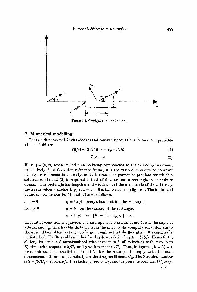
FIGURE 1. Configuration definition.

2. Numerical modelling

viscous fluid are The two-dimensional Navier-Stokes and continuity equations for an incompressible

( 1 )

v . q = 0. (2)

aq/at + (q . v) q = - vp + m q ,

Here q = (u ,v) , where u and v are velocity components in the x- and y-directions, respectively, in a Cartesian reference frame, p is the ratio of pressure to constant density, v is kinematic viscosity, and t is time. The particular problem for which a solution of (1) and (2) is required is that of flow around a rectangle in an infinite domain. The rectangle has length a and width b, and the magnitude of the arbitrary upstream velocity profile U(y) a t x = y = 0 is U,, as shown in figure 1 . The initial and boundary conditions for ( 1 ) and (2) are as follows:

at t = 0 ;

for t > 0

q = U(y)

q = 0

everywhere outside the rectangle

on the surface of the rectangle,

q+U(y) as 1x1 = I(X-X,,y)I-tOo.

The initial condition is equivalent to an impulsive start. I n figure 1 , a: is the angle of attack, and xR, which is the distance from the inlet to the computational domain to the upwind face of the rectangle, is large enough so that the flow at x = 0 is essentially undisturbed. The Reynolds number for this flow is defined as R = U,b/v. Henceforth, all lengths are non-dimensionalized with respect to b, all velocities with respect to U,, time with respect to b/U,, and p with respect to U;. Thus, in figure 1, b = U, = 1 by definition. Then the lift coefficient C, for the rectangle is simply twice the non- dimensional lift force and similarly for the drag coefficient, C i . The Strouhal number is S = fb/U,, = f, where f is the shedding frequency, and the pressure coefficient C, is 2p.

16-2

478 R. W . Davis and E . F . Moore

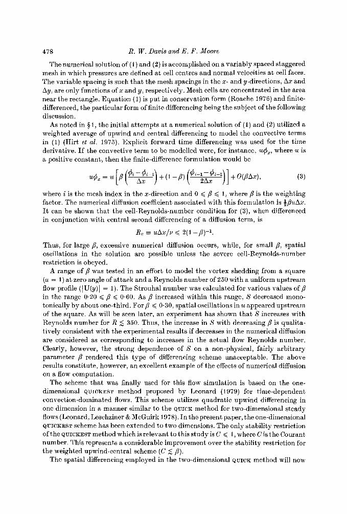
The numerical solution of (1) and (2) is accomplished on a variably spaced staggered mesh in which pressures are defined a t cell centres and normal velocities a t cell faces. The variable spacing is such that the mesh spacings in the x- and y-directions, Ax and Ay, are only functions of x and y, respectively. Mesh cells are concentrated in the area near the rectangle. Equation (1) is put in conservation form (Roache 1976) and finite- differenced, the particular form of finite differencing being the subject of the following discussion.

As noted in $1, the initial attempts a t a numerical solution of ( 1 ) and (2) utilized a weighted average of upwind and central differencing to model the convective terms in ( 1 ) (Hirt et al. 1975). Explicit forward time differencing was used for the time derivative. If the convective term to be modelled were, for instance, u # ~ , where u is a positive constant, then the finite-difference formulation would be

where i is the mesh index in the x-direction and 0 < < 1, where /3 is the weighting factor. The numerical diffusion coefficient associated with this formulation is BPuAx. It can be shown that the cell-Reynolds-number condition for (3), when differenced in conjunction with central second differencing of a diffusion term, is

R, U A X / V < 2( 1 -/?)-I.

Thus, for large p, excessive numerical diffusion occurs, while, for small P, spatial oscillations in the solution are possible unless the severe cell-Reynolds-number restriction is obeyed.

A range of p was tested in an effort to model the vortex shedding from a square ( a = 1) at zero angle of attack and a Reynolds number of 250 with a uniform upstream flow profile (IU(y)l = 1). The Strouhal number was calculated for various values of ,4 in the range 0.20 < p < 0.60. As p increased within this range, S decreased mono- tonically by about one-third. For /3 < 0-30, spatial oscillations in u appeared upstream of the square. As will be seen later, an experiment has shown that S increases with Reynolds number for R 5 350. Thus, the increase in S with decreasing ,4 is qualita- tively consistent with the experimental results if decreases in the numerical diffusion are considered as corresponding to increases in the actual flow Reynolds number. Clearly, however, the strong dependence of S on a non-physical, fairly arbitrary parameter p rendered this type of differencing scheme unacceptable. The above results constitute, however, an excellent example of the effects of numerical diffusion on a flow computation.

The scheme that was finally used for this flow simulation is based on the one- dimensional QUICKEST method proposed by Leonard (1 979) for time-dependent convection-dominated flows. This scheme utilizes quadratic upwind differencing in one dimension in a manner similar to the QUICK method for two-dimensional steady flows (Leonard, Leschziner & McGuirk 1978). I n the present paper, the one-dimensional QUICKEST scheme has been extended to two dimensions. The only stability restriction of the QUICKEST method which is relevant to this study is C < 1, where Cis the Courant number. This represents a considerable improvement over the stability restriction for the weighted upwind-central scheme (C 5 p).

The spatial differencing employed in the two-dimensional QUICK method will now

Vortex shedding from rectangles 479

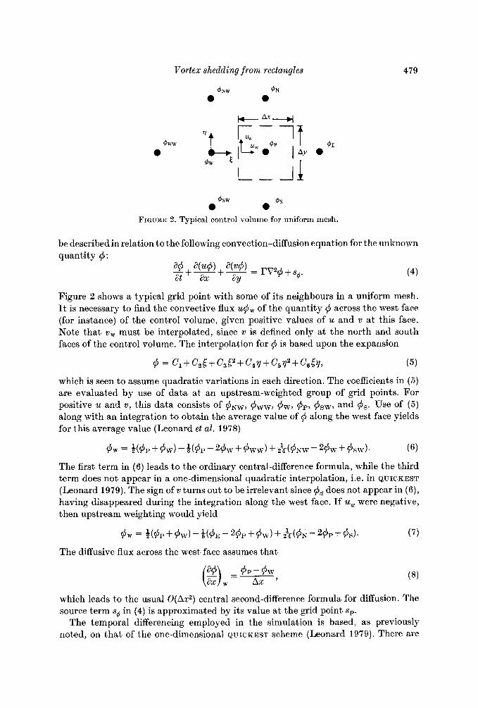
FIGURE 2. Typical control volume for uniform mesh.

be described in relation to the following convection-diffusion equat,ion for the unknown quantity 4:

Figure 2 shows a typical grid point with some of its neighbours in a uniform mesh. It is necessary to find the convective flux u$w of the quantity 4 across the west face (for instance) of the control volume, given positive values of u and v a t this face. Note that vw must be interpolated, since 2, is defined only at the north and south faces of the control volume. The interpolation for 4 is based upon the expansion

4 = c,+c2~+c,52+c4r+cgr2+c6~rl, ( 5 )

which is seen to assume quadratic variations in each direction. The coefficients in ( 5 ) are evaluated by use of data a t an upstream-weighted group of grid points. For positive u and v, this data consists of q&, q5ww, &, &,, 4sw, and ds. Use of ( 5 ) along with an integration to obtain the average value of q5 along the west face yields for t’his average value (Leonard et al. 1978)

4 w = i ( 4 P + 4 w ) - S(4P - 24w + 4w7w) + +d4,.w - 24w + 4sw). (6)

The first term in (6) leads to the ordinary central-difference formula, while the third term does not appear in a one-dimensional quadratic interpolation, i.e. in QUICKEST

(Leonard 1979). The sign of v turns out to be irrelevant since 4s does not appear in (6) , having disappeared during the integration along the west face. If u, were negative, then upstream weighting would yield

4 w = H 4 P + 4w) - Q ( 4 E - 24P + 4M7) + +d4x - 24P + 4s). (7)

The diffusive flux across the west face assumes that

4 P - 4 w (g),= Ax ’

which leads to the usual O(Ax2) central second-difference formula for diffusion. The source term s+ in (4) is approximated by its value a t the grid point sp.

The temporal differencing employed in the simulation is based, as previously noted, on t’hat of the one-dimensional QUICKEST scheme (Leonard 1979). There are


several ways of deriving this type of differencing scheme. Leonard employed convective integrations in which space replaced time as the integration variable, i.e. dx = udt. A simpler way of deriving the QUICKEST scheme which more clearly shows the approximations involved is to replace the time derivatives in a Taylor expansion with space derivatives. Consider the following source-free convection-diffusion equation in one dimension :

-+u- a4 84 = r- a24 at ax ax2 9

where r and u are constants. Expand qi about time level N to obtain

where t = NAt. Then, from (9))

(9)

where, since the spatial finite-difference approximations to be used contain fourth derivatives in their leading truncation errors, the generally small (being multiplied by I') fourth- and higher-spatial-derivative terms have been dropped from (1 1). Inserting (9) and ( 1 1) into (10) gives

a3+ N ++At3(-u3@)I . (12)

Spatial discretization about grid point i is accomplished by first fitting a quadratic across grid points i + 1, i , and i - 1 , and then integrating to obtain the average value of $ within the i th mesh cell. This average value is determined a t time levels N and N + 1, thus yielding r#N and $Iv+l. The difference ( 4 d V + l - 4 ~ ~ ) becomes

4 N+1- 4 N = 4 ~ + 1 - 4 ~ + ~ ~ [ ( 4 ~ ~ 1 - 2 4 ~ + l + 4 ~ ~ ~ 1 ) - ( 4 ; y , 1 - 2 4 ~ + 4 ~ 1 ) ] . (13)

The last two terms in ( I 3) can be interpreted as

from (9). Discretization in the manner previously described for QUICK is then applied to the spatial derivatives in (12) and (14) to finally obtain

$?+I = @ - &c(q5$$l - $El) + (y + iC2) ($S1 - 24T + $El) +C(+-y-+CZ) ( $ ; . + 1 - 3 4 ~ + 3 ~ ~ - 1 - 4 ~ ~ 2 ) , (16)

where C = uAt /hx and y = I'At/Ax2. Equation (15 ) is third-order accurate both temporally and spatially as --f 0. For small y , i t is stable for C d 1 (Leonard 1979).

Similarly, in two dimensions either convective integrations or a Taylor-series expansion in time can be straightforwardly applied to obtain a finite-difference approximation to (4). I n these derivations, only normal, and not tangential, diffusion is considered a t each control voliime face in figure 2, Also sc is treated as a constant


for each control volume. The two methods of derivation lead to identical results except for the presence on the right-hand side of (16) of some O(At2) spatial cross- derivative terms which appear only when the Taylor expansion is used. With these terms omitted for simplicity, the resulting finite-difference equation is

@+' = $$ + { - Q e [&(#p -I- 9 ~ ) - i c e ( & -$PI - (8 -YE- Qci) ($E - 2 4 ~ + &)I + CW[i(9, + 9w) - iCW(9P - 9w) - ( 8 - Y z - QQ:") (9ww - 29w + 9r)l- C,[ i (9P + 9 N )

- HCn(9, - 9d - (Q - Y1/ - QG) ($N - 2 9 P + &)I + Qf"P + 9s) - i Q d $ P - $s) - (Q --I?/ - -m ( 9 P - 29s + 9ss)l + Y J $ E - 29P + 9w) + YJ9N - 2 9 P + 4s ) + SP A t Y . (16)

In (16), the Cs are the Courant numbers (all assumed positive) at the various control- volume faces in figure 2 ; yz = FAt/Ax2 and yU = I'At/Ay2. Note that, because of two-dimensional spatial averaging within grid cells (as per (13) in one dimension), q5NW, &w, and q5SE do not appear in (16). It is (16), appropriately modified for a non-uniform grid, that is used to approximate the momentum equations (1). Owing to the small time steps employed, the effect of the neglected cross-derivatives on the numerical results was negligible, although their omission formally reduces the temporal accuracy of (16) as r-+O to O(At ) . The spatial accuracy as I'+O remains O(Ax3, Ay3) . Since the computed velocity field at a given time step will probably not satisfy the continuity equation (2), it is necessary to adjust this field. The adjustment procedure will be discussed next.

The velocity divergence for a given control volume is driven approximately to zero by adjusting the control volume pressure pp. This pressure adjustment produces a corresponding velocity adjustment, which for the u-component of velocity is determined from

Sue At Su, At 8pP Ax' 8pP Ax' (17) - = - - =--

where Su and Sp are the velocity and pressure increments. This adjustment process, which amounts to solving a Poisson equation for the pressure, is performed iteratively by successive over-relaxation until the sum of the absolute values of the mass residuals over all mesh cells is less than e times the inlet mass flow (Hirt et al. 1975). Finally, the pressure at the origin is set to zero.

The boundary conditions used in this simulation will now be described. The upstream undisturbed velocity profile U ( y ) is specified at x = 0 in figure 1, thus deter- mining the angle of attack a. The free-stream velocity is specified a t y = yim for all x. The situation a t the exit from the computational mesh is more complex. Use of zero-gradient boundary conditions here causes premature smoothing of the wake. Thus, as done previously by Lugt & Haussling (1974) and Mehta & Lavan (1975), the computation of local velocities a t the exit was selected as the best method of allowing vortices to leave the domain with minimal interference. I n order to reduce extrapolations to a minimum, the differencing of ( 1 ) a t the exit is accomplished by ignoring the diffusion terms and employing first-order upwind differencing on the convective terms. For the computation of the u-component of velocity a t the exit by this method, v a n d p are linearly extrapolated over a distance Ax downstream of their exit locations.


r - i

r - i

( b ) ( C )

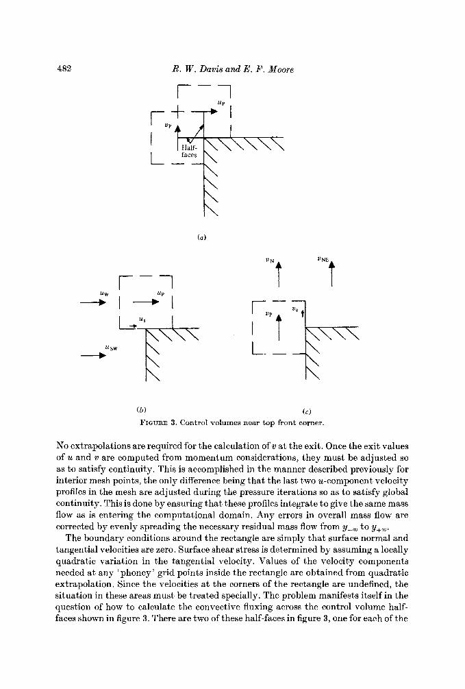
FIGURE 3. Control volumes near top front corner.

No extrapolations are required for the calculation of v a t the exit. Once the exit values of u and v are computed from momentum considerations, they must be adjusted so as to satisfy continuity. This is accomplished in the manner described previously for interior mesh points, the only difference being that the last two u-component velocity profiles in the mesh are adjusted during the pressure iterations so as to satisfy global continuity. This is done by ensuring that these profiles integrate to give the same mass flow as is entering the computational domain. Any errors in overall mass flow are corrected by evenly spreading the necessary residual mass flow from y--m to Y + ~ .

The boundary conditions around the rectangle are simply that surface normal and tangential velocities are zero. Surface shear stress is determined by assuming a locally quadratic variation in the tangential velocity. Values of the velocity components needed a t any 'phoney' grid points inside the rectangle are obtained from quadratic extrapolation. Since the velocities at the corners of the rectangle are undefined, the situation in these areas must be treated specially. The problem manifests itself in the question of how to calculate the convective fluxing across the control volume half- faces shown in figure 3. There are two of these half-faces in figure 3, one for each of the


control volumes surrounding the velocities nearest the front corner shown. The convective fluxing across these half-faces a t the front corners of the rectangle is accomplished by ( 1 ) assuming an average normal velocity across these half-faces equal to that a t the outer edge of the half-face (i.e. using vp for the normal velocity across the u-control volume’s half-face and vice versa), and (2) assuming that the fluxed quantity (us and v, in figures 3b, c) satisfies a linear fit a+bx+cy through the nearest three non-zero nodal values of the respective velocity component shown in figures 3 (b , c ) . Since the signs of the velocity components at the front corners do not vary with time, no provision need be made for this (e.g. changing the nodal values for the linear fit). The situation at the rear corners is different, since the velocities there change direction during the shedding cycle. Consequently, the convective fluxing across the rear corner half-faces is accomplished in the same manner as for interior cells (quadratic upwinding) with the addition of some linear interpolations to obtain values of the fluxed quantity a t the centre of each of the half-faces. Normal velocities across rear half-faces are determined in the same manner as for front half-faces. The procedures just described a t the four corners are obviously not the only possible ones. They do, however, lead to slightly better results than various other procedures that were tested, such as quadratic upwinding at all four corners. Research is clearly needed on the numerical treatment of flows near sharp corners. One such effort by Ghia & Davis ( 1974) employed similarity variables in conjunction with a conformal transformation in order to study the steady flow around a semi-infinite rectangular slab. A comparison between results obtained by them and some present results will be made subsequently.

The non-uniform computational meshes employed in this study ranged in size from 41 x 40 to 61 x 74, with the first number being the number of mesh points in the x-direction and the second in the y-direction. The value selected for \y*ml for a = 0 was 6, larger values having an insignificant effect on vortex street development and on quantities such as Strouhal number, lift and drag. The value for xR was 4.5, while values of x a t the exit from the mesh ranged from 15 to 20. The divergence criterion E

was set a t 2 x values ten times less or five times greater effecting negligible changes in the results. The initial conditions for the computations were either a uniform flow everywhere (impulsive Start) or the results of a previous calculation, often a t a different Reynolds number. The time step At was generally set a t 0.05 so as to maintain the maximum Courant number in the flow a t less than unity. Computation times on the NBS UNIVAC 1108 ranged up to 24 hours for the finest mesh starting from a uniform flow everywhere. Generally, nine hours of computation time sufficed to obtain constant-Strouhal-number vortex shedding when using results of a previous calculation as initial conditions. When starting from a uniform initial flow everywhere, vortex shedding would begin spontaneously after a while, with no upstream perturba- tion required.

3. Results and discussion Using the previously described numerical method, computations have been carried

out for flow around various rectangles. The parameters involved are a, R, a, and (U(y)/ . Table 1 shows the combinations of these parameters that were tested. The initial configuration was a square a t zero angle of attack with a uniform upstream velocity profile and Reynolds numbers between 100 and 2800. For this configuration,


Configuration a R a IU(Y)l 1 1 100-2800 0 1 2A 1 250; 1000 5" 1 2B 1 250; 1000 15' 1 3 1 250; 1000 0 1 + 0.1oy 4A 0.6 250; 1000 0 1 4B 1.7 250; 1000 0 1

TABLE 1. Computed parameter combinations

+ m x

A d

d

0.16 O F :

O + X

1 0.1 3

A

+ x 0 a A

A a + + x d

+ X +

x x + + +

0.1 2 100 500 1000

R

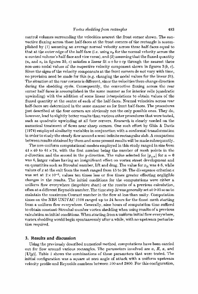
FIGURE 4. Numerical-experimental Strouhal-number comparison for configuration 1. Computed: 0, 41 x 40 grid; A , 51 x 62; 61 x 74. Experimental: x , run 1; +, run 2.

Strouhal number and average and r.m.s. values of the lift and drag coefficients were computed over the aforementioned Reynolds-number range. The Strouhal numbers were compared with the results of a wind-tunnel test, which will now be described.

A 3.175 mm (0.125 in.) square steel rod was mounted in the test section of the NBS Low Velocity Airflow Facility (Purtell & Klebanoff 1979), with the rod spanning the tunnel horizontally (0.94 m). The rod was normal to the flow in a region of constant velocity (outside the wall boundary layers), zero streamwise pressure gradient, and free-stream turbulence intensity of less than 0.05 yo. The free-stream velocity was measured by a Pitot-static tube. A 2.5 pm by 1 mm hot wire was placed parallel to the rod at selected positions attained by a traverse and checked by a cathetometer from outside the tunnel during testing. The signal from the hot-wire anemometer was observed on an oscilloscope and the vortex-shedding frequency estimated. This frequency was then more accurately determined by a digital averaging counter.


I’

l . 1 1.7

A

A

CI

A

0

A 0

0

A

c)

a 0

1.6 1 I I 100 500 1000

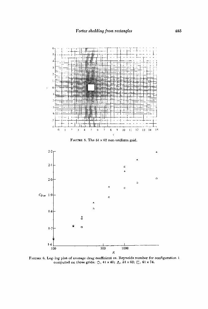
R FIQURE 6. Log-log plot of average drag coefficient vs. Reynolds number for configuration 1

computed on three grids: 0, 41 x 40; A, 51 x 62; m, 61 x 74.

486 R. W . Davis and E . F. Moore

0.60

0

-0.60

CL

- 1.20

-1.80, (

2.00

0

CL -2.00

-4.00

-6.00

I I I I I I I I

2 4 6 8 10 12 14 16 18 20 22 24 1 . . . . . . . 1l1.71

Time

7 3.35

2.95

2.5 5

2.15

1.75 2 4 6 8 10 12 14 16 18 20 22 24 26 28

CD

Time

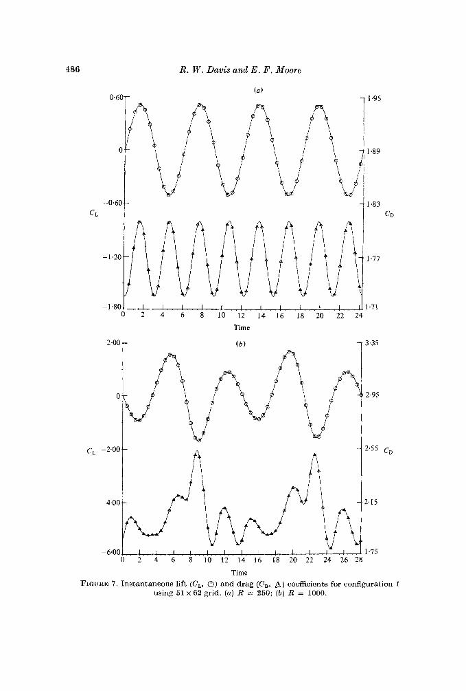
FIGURE 7. Instantaneous lift (CL, 0) and drag (CD, A ) coefficients for configuration 1 using 51 x 62 grid. ( a ) R = 250; ( b ) R = 1000.


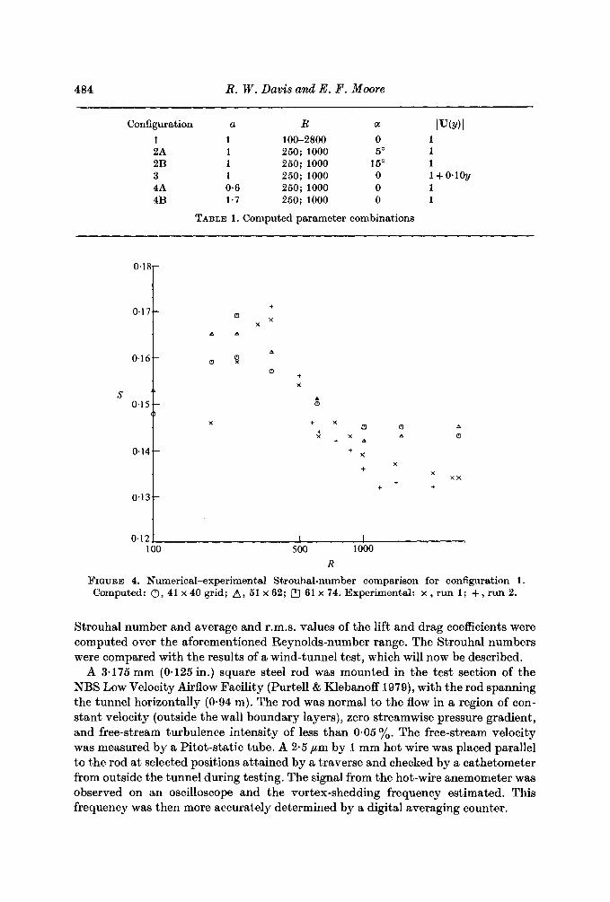
The computed and experimental values of Strouhal number for configuration 1 are shown as functions of Reynolds number in figure 4. The experimental values are shown for two test runs, thus giving an idea of the experimental uncertainty. The computed values were calculated on three non-uniform meshes, 41 x 40, 51 x 62, and 61 x 74, with the second one being shown in figure 5. These computed frequencies are based on the periodic fluctuations of the following four quantities: (1) the v-component of velocity on the centreline just off the rear face of the rectangle, (2) the y-co-ordinate of the stagnation point just off the front face of the rectangle, (3) the lift coefficient, and (4) the u-component of velocity at the downstream location where the wind-tunnel measurements were made. The fluctuations were allowed to reach a steady state before an average frequency was determined over approximately 4 cycles of each of these quantities. These four frequencies (generally within 3 % of each other) were then averaged to obtain the plotted values. The regularity of the fluctuations with time once steady-state vortex-shedding was reached is a function of Reynolds number and will be discussed below. It is clear from figure 4 that the three grids give very similar results and are in generally good agreement with the experimental resultsfor R < 1000. The 61 x 74 grid (with At = 0.025) was used at only two Reynolds numbers because of limited computer resources. The other two grids and the experiment show S peaking in the neighbourhood of R = 300. For R > :OOO, the computational and experimental results are no longer in qualitative agreement, with the numerical simulation failing to predict the continued decline in S with increasing R. It is noted, for reference, that for R = O( lo5) the Strouhal number is about 0.12 (Vickery 1966).

Also, as discussed previously, quadratic upwinding was tried at the four corners of the square and led to values of S about 7 % lower than those shown for R < 1000. This was clearly less satisfactory in predicting the behaviour of S in this Reynolds- number regime.

against Reynolds number for configuration 1 is presented in figure 6, with the computations once again being carried out on the three meshes mentioned previously. The plotted drag coefficients are based only upon pressure drag, as viscous-drag effects were negligible. As can be seen from figure 6, the average drag coefficient increases with Reynolds number, the rate of increase being greater with the 51 x 62 grid than with the 41 x 40 grid. For R < 1000 the differences among the three grids are less than 7 %. For reference, the average drag coefficient for smooth flow at high R [0( lo5)] is about 2.2 (Lee 1975). The average lift coefficient for configuration 1 was O( 10-2) or less.

Figures 7 (a, b ) present plots of computed instantaneous lift and drag coefficients, C , and C,, against time for configuration 1 at Reynolds numbers of 250 and 1000 after steady-state vortex shedding has been reached. Once again viscous effects are ignored in these coefficients, which were computed using the 51 x 62 grid. Although these plots (and figures 11 and 13 below) were constructed from data at each time step, the symbols are plotted only every ten time steps. The difference in the appearance of these two plots is striking, with figure 7 (a ) being a simple sine wave while figure 7 ( b ) shows the effects of harmonics appearing at the larger Reynolds number. Note that one period in the shedding cycle (two vortices shed) remains as the time between adjacent peaks in the lift curve regardless of amplitude variations. The appearance of the subharmonic in C , at R = 1000 signifies small modulations in shedding frequency which do not occur at R = 250. The drag, of course, oscillates at twice the frequency

A log-log plot of computed average drag coefficient C ,


=.

I

Y

-1 2. ,c

Y

. ?

c .II

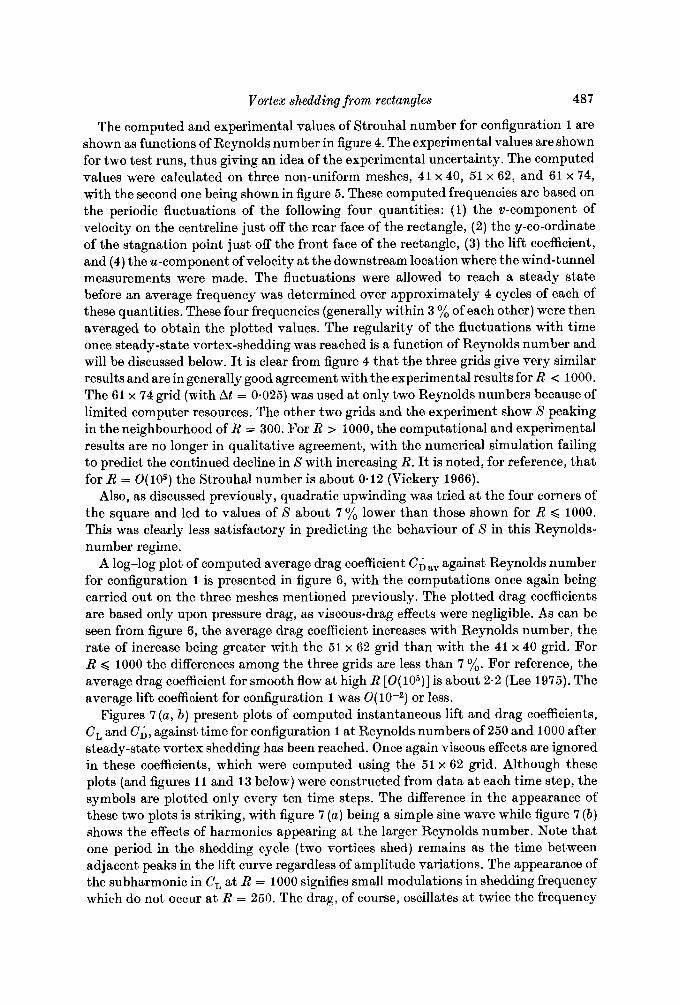
I FIGURE 8. Streakline plots for configuration 1 using 61 x 74 grid.

(a ) R = 250; ( b ) R = 1000.

of the lift. Root-mean-square values of the lift and drag coefficients will be presented later in a summary table for all the tested configurations. It is noted that the behaviour of the front-face stagnation point and rear-face centre-line vertical velocity component v is virtually identical to that of C, in figures 7 (a, b ) . The front-face stagnation point traverses the central 6 % of the face at R = 250 and 20 % at R = 1000.

Figures 8 (a, b ) are streakline plots of typical vortices for configuration 1 at Reynolds numbers of 250 and 1000 utilizing the 61 x 74 grid. The flow visualizers here are passive marker particles introduced ahead of the body, a different symbol being used for each approaching streakline. There are 14 streaklines with new particles being


3

1

Y

-1

-3

(a)

......... * . .. ..... .... ....... ...tv::::,+ri;.......'.:: ....... . . . . . : - m . . . * * * -.- ............... .....

............................ '._ m..Q".. a.

-.. .......

...........

..*-" .........

! I 1 I , . - , ! I 4 6 8 10 12 14

X

't

-5 4 6 8 10 12 14

X

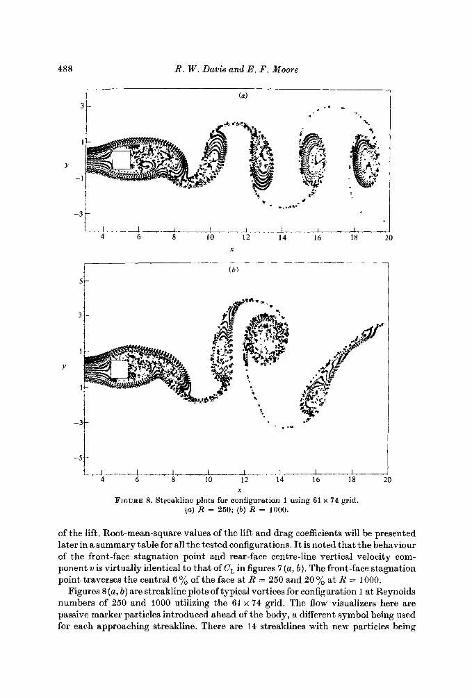
FIGURE 9. Particle trajectories for configuration 1 using 51 x 62 grid. (a) R = 250; (6) R = 1000.

injected at time intervals of 0.10. At time t + At a given particle is moved a distance IqI At in the appropriate direction. The velocity q here is obtained by linear interpolation among the surrounding grid points. This is done at both time t and time t + At and then the two qs are averaged to obtain the particle velocity over the time span At. The particles are swept into the vortices behind the body and are shed with them, thus providing an excellent means for visualizing the motion of these large coherent structures as they move downstream away from the body. It will be seen


Y

3

1

-1 6 8 10 12 4

1 .so

0

CL -1.50

-3.00

-4.5c

X

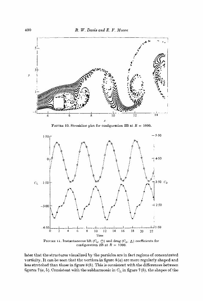
FIGURE 10. Streakline plot for configuration 2B at R = 1000.

7 5.50

4.50

3.50 CD

2.50

! . ! . . ! , . ! . . , L . , ! . . ! . , . I . ! , . ! . _ . I 1.50 2 4 6 8 10 12 14 16 18 20 22

Time

FIGURE 11. Instantaneous lift (CL, 0) and drag (GI,, A ) coefficients for configuration 2B at R = 1000.

later that the structures visualized by the particles are in fact regions of concentrated vorticity. It can be seen that the vortices in figure 8 (a) are more regularly shaped and less stretched than those in figure 8 (b) . This is consistent with the differences between figures 7 (a, b). Consistent with the subharmonic in C , in figure 7 ( b ) , the shapes of the

Vortex shedding from rectangles 49 1

Y

I I ! I I 4 6 8 10 12 14

I .- -3

X

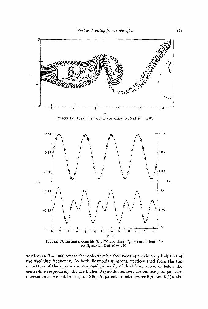
FIGURE 12. Streakline plot for configuration 3 a t R = 250.

-0.85 1.85

-1.35 1.75

-1-85 1.65

Time

FIGURE 13. Instantaneous lift (CL, 0) and drag (CD, A ) coefficients for configuration 3 at R = 250.

vortices a t R = 1000 repeat themselves with a frequency approximately half that of the shedding frequency. At both Reynolds numbers, vortices shed from the top or bottom of the square are composed primarily of fluid from above or below the centre-line respectively. At the higher Reynolds number, the tendency for painvise interaction is evident from figure 8 ( b ) . Apparent in both figures 8 (a) and 8 ( b ) is the

492

Y

R. W . Davis and E . F. Moore

7

-3 t t ! I I I , , , I . , , . , , I , , ,

4 6 8 10 12 14

X

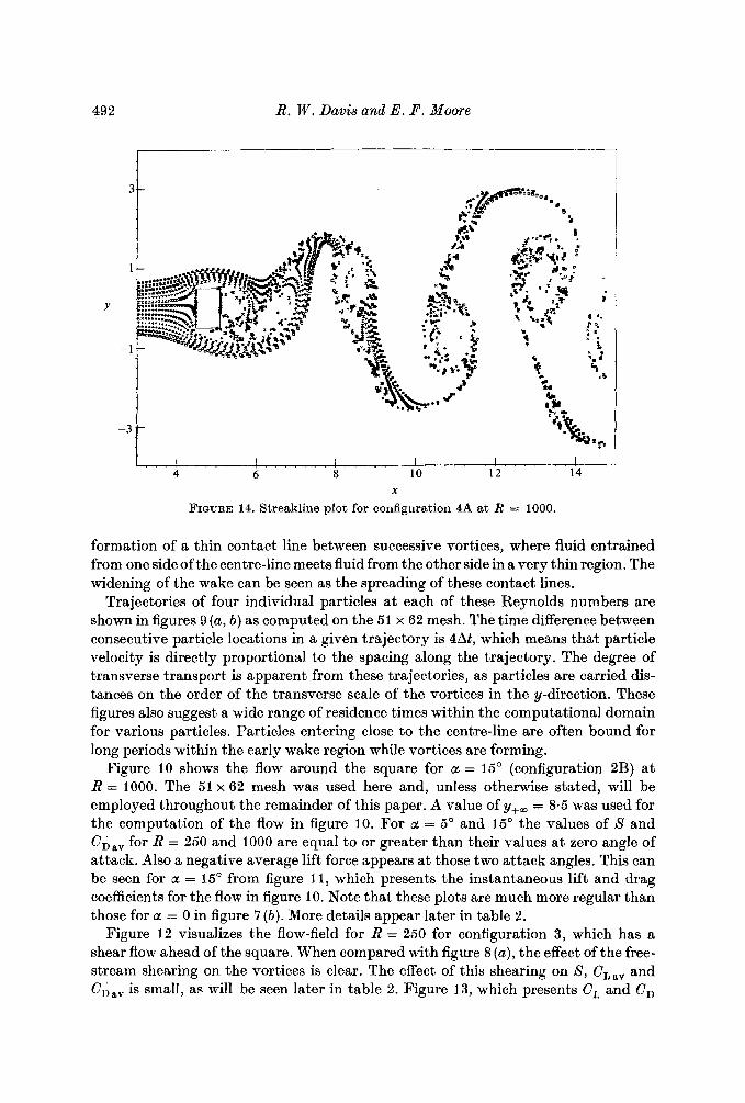
FIGURE 14. Streakline plot for configuration 4A at R = 1000.

formation of a thin contact line between successive vortices, where fluid entrained from one side of the centre-line meets fluid from the other side in a very thin region. The widening of the wake can be seen as the spreading of these contact lines.

Trajectories of four individual particles at each of these Reynolds numbers are shown in figures 9 (a, b ) as computed on the 51 x 62 mesh. The time difference between consecutive particle locations in a given trajectory is 4At, which means that particle velocity is directly proportional to the spacing along the trajectory. The degree of transverse transport is apparent from these trajectories, as particles are carried dis- tances on the order of the transverse scale of the vortices in the y-direction. These figures also suggest a wide range of residence times within the computational domain for various particles. Particles entering close to the centre-line are often bound for long periods within the early wake region while vortices are forming.

Figure 10 shows the flow around the square for a = 15' (configuration 2B) at R = 1000. The 51 x 62 mesh was used here and, unless otherwise stated, will be employed throughout the remainder of this paper. A value of y+03 = 8.5 was used for the computation of the flow in figure 10. For a = 5' and 15' the values of S and Ciav for R = 250 and 1000 are equal to or greater than their values a t zero angle of attack. Also a negative average lift force appears at those two attack angles. This can be seen for a = 15' from figure 11, which presents the instantaneous lift and drag coefficients for the flow in figure 10. Note that these plots are much more regular than those for a = 0 in figure 7 ( b ) . More details appear later in table 2.

Figure 12 visualizes the flow-field for R = 250 for configuration 3, which has a shear flow ahead of the square. When compared with figure 8 (a), the effect of the free- stream shearing on the vortices is clear. The effect of this shearing on s, C,,, and C1iav is small, as will be seen later in table 2. Figure 13, which presents C , and C ,


1

Y

-1

1 I I I 1 I I , , 1 4 6 8 10 12 14 16

X

I I , , I I _ , , . I , , , , , ,

4 6 8 10 12 14 X

3 c

1 Y

-1

I

-3 ! I I I , . . I t , , . . 4 6 8 10 12 14 1

X

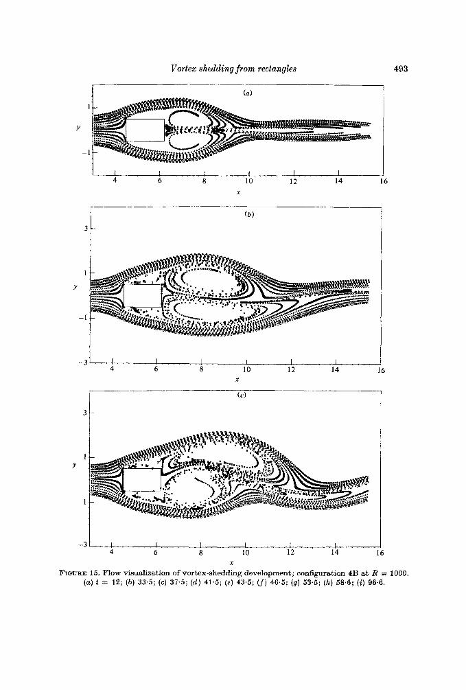
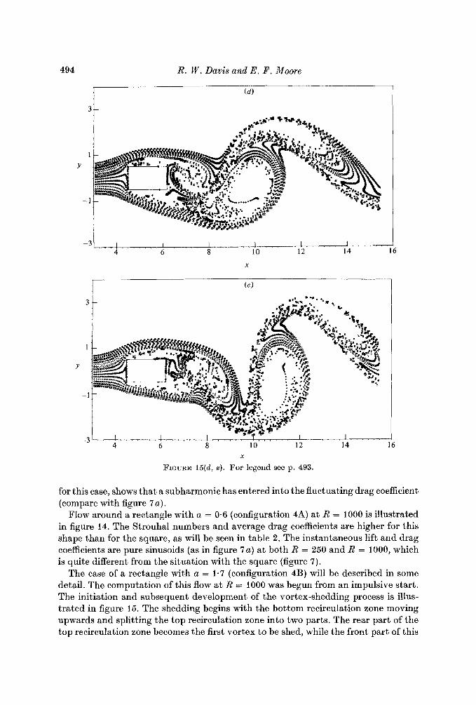
FIGURE 15. Flow visualization of vortex-shedding development; configuration 4B at R = 1000. (a) t = 12; (b ) 33.5; (c ) 37.5; ( d ) 41-5; ( e ) 43-5; (f) 46.5; (9) 53.5; (h) 58.6; ( i ) 96.6.

494 R. W . Davis and E . F. Moore

1

Y

-1

-31 I I I I I I , , ,

4 6 8 10 12 14

X

Y

3

1

-1

4 6 8 10 12 14 -3

X

FIGURE 15(d, e). For legend see p. 493.

- 16

6

for this case, shows that a subharmonic has entered into the fluctuating drag coefficient (compare with figure 7 a ) .

Flow around a rectangle with a = 0.6 (configuration 4A) a t R = 1000 is illustrated in figure 14. The Strouhal numbers and average drag coefficients are higher for this shape than for the square, as will be seen in table 2. The instantaneous lift and drag coefficients are pure sinusoids (as in figure 7 a ) a t both R = 250 and R = 1000, which is quite different from the situation with the square (figure 7) .

The case of a rectangle with a = 1.7 (configuration 4B) will be described in some detail. The computation of this flow a t R = 1000 was begun from an impulsive start. The initiation and subsequent development of the vortex-shedding process is illustrated in figure 15. The shedding begins with the bottom recirculation zone moving upwards and splitting the top recirculation zone into two parts. The rear part of the top recirculation zone becomes the first vortex to be shed, while the front part of this

Vortex shedding from rectangles

5 0

I I , , I I - 5 . . - ! . . . . ! .

Y

c

1

3c

Y

-1

I

495

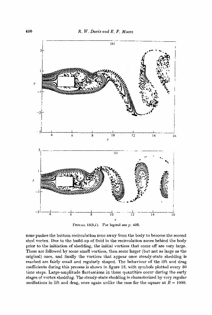
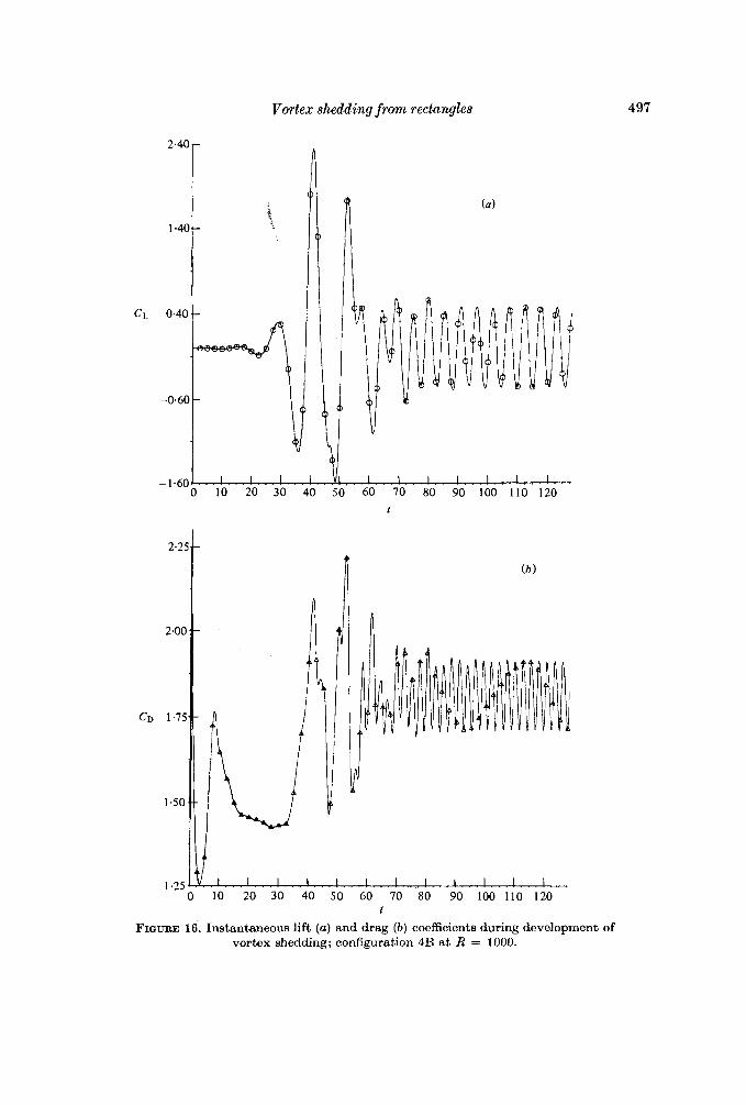
*ooo[ = 2 qo amnbs ayq .103 asm arp aygun up8o aauo '8o.1~ pus $311 u~ suoyqpso mIn8aJ han dq pazpaqoosoyo s! 8u!ppays aqoqs-dpsaqs ay;C -8uIppays xaqaon JO sa8oqs dpoa ay$ Bu!Jnp xnooo sayqusnb asayq ui suoyonqong apnqgdmo-a8m? .sdaqs amy 09 hana paqqold sloqmds Y+'M '91 am8y u~ UMO~S s! ssaoo.xd sryq 8urmp squapgaoo 8s~p pus 3311 ayq 30 anopwyaq ay;C .padsys dpqn8a;r pus pms Lp33 am payooan sr kppays aqoqs-dpoaqs aouo maddo qsyq sao!qJon ayq dpuy puo 'sauo (~ou@po ayq so a8.q so qou qnq) ~a8.1~1 amos uayq 'sao!qaon 11ou1s amos 6q pa~o~~oj am asay;C *aBJoI han am 30 amoo qoyq saoyJon pqu! ayq '8mppays 30 uopypq ayq oq aopd dpoq ayi puyaq sauoz uoyoIn3.qoa.I ayq UI pg 30 dn-ppq ayq oq ana 'xaqaon pays puooas ayq aurooaq oq dpoq ayq u10.13 LVMQ auoz uoyqnoapaa Uroqqoq ayq saysnd auoz

I I I I .p ' E- PI , ZI ,or, , 8,. , , 9

i' "' I

tS-

E-

I-

A

I

E

96V

2.40

1.40

CL 0.40

-0.60

-1.60

2.2f

2.00

CD 1.75

1 .so

1.25


R . . . . . . . . . I I ! , . . ! , . ~ ~ , , . ! . , ! . . . ! . . ! . . ! . . . ' . . . ! . . ,

10 20 30 40 50 60 70 80 90 100 110 120

t

( b )

FIGURE 16. Instantaneous lift (a) and drag (b) coefficients during development of vortex shedding; configuration 4B at R = 1000.

498

3

1

-1-

-3-

R. W . Davis and E . F. Moore

.-

I-

4 6 8 10 12 14

X

Y

j , , , ! , , , , , , , ! , , , , , , , ! , , , , , , ~! / , , , , , , ! , , , , , , , ! , , , , , 4 6 8 10 12 14

X

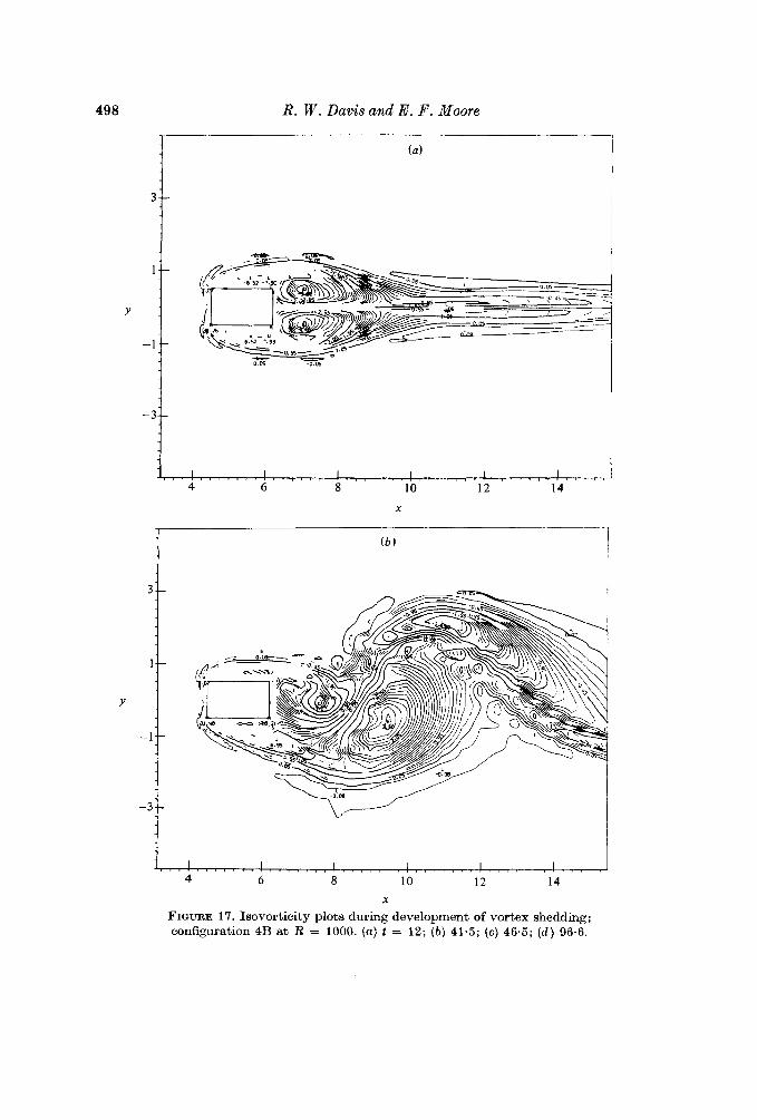
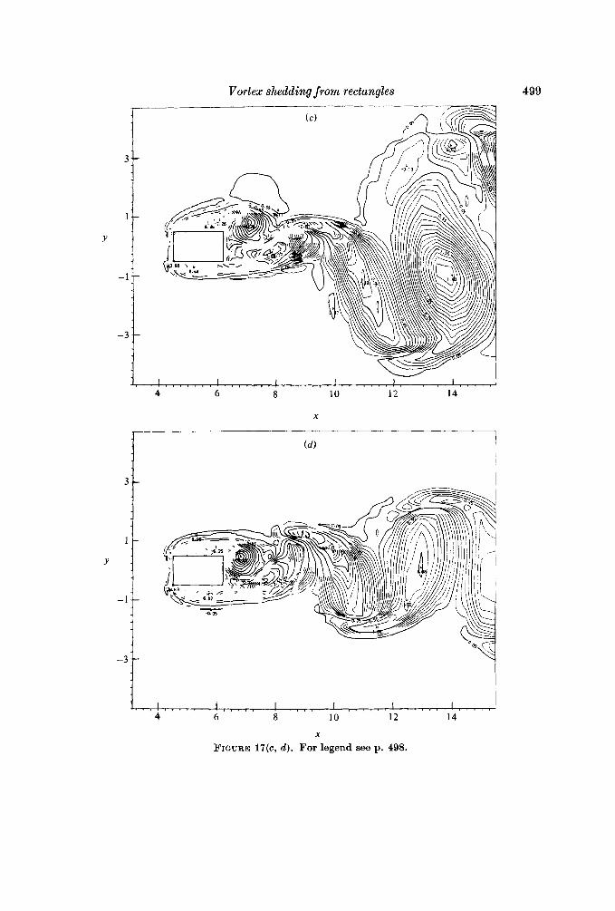
FIGURE 17. Isovorticity plots during development of vortex shedding; configuration 4B at R = 1000. (a) t = 12; ( b ) 41.5; ( c ) 46.5; ( d ) 96.6.


Y

4 6 8 10 12 14

X

- 1 I Y

i -31

\

i , , , ! , , , , , , , ! , , , , , , , ! , , , , / , , I , , , , , , , ! , , , , , , , 1 , . , ,

4 6 8 10 12 14

X

FIGURE 17(c, d) . For legend see p. 498.


Y

-2 I Y

4 6 8 X

X

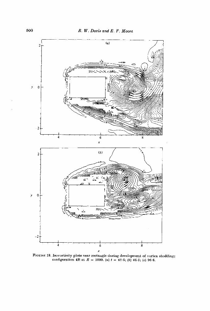
FIGURE 18. Isovorticity plots near rectangle during development of vortex shedding; configuration 4B at R = 1000. (a) t = 41.5; ( b ) 46.5; ( c ) 96.6.


Y 0..

-2 --

Y

4 6 8

X

FIGURE 18(c). For legend see p. 500.

- 1

-g I,..! , , . , ( , I ! , , , , ! , , ! , ~ , . , > , ! , - < , , , . ! , , , , , , , ! , / . , ,

4 6 8 10 12 14 X

FIGURE 19. Overlay of streakline plot on isovorticity plot after development of vortex shedding; configuration 4B a t R = 1000.

502 R. W . Davis and E. F . Moore

0

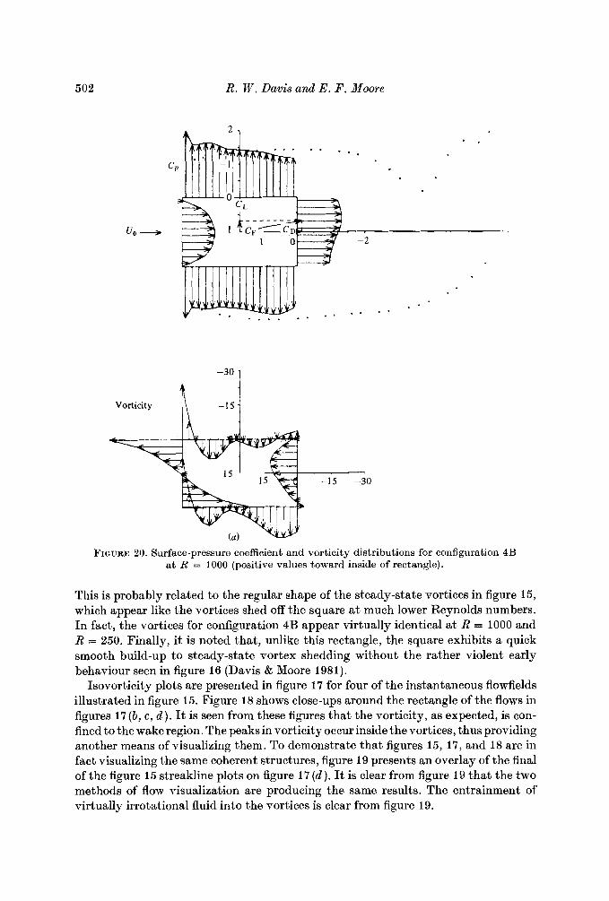
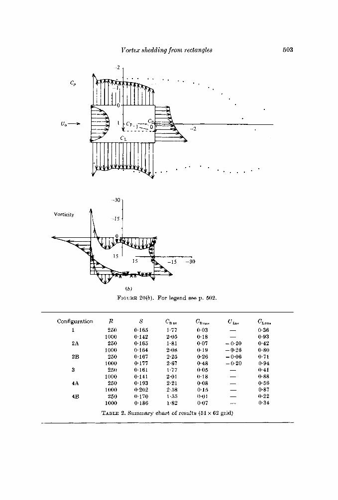
FIGURE 20. Surface-pressure coefficient and vorticity distributions for configuration 4B at R = 1000 (positive values toward inside of rectangle).

This is probably related to the regular shape of the steady-state vortices in figure 15, which appear like the vortices shed off the square at much lower Reynolds numbers. In fact, the vortices for configuration 4B appear virtually identical at R = 1000 and R = 250. Finally, i t is noted that, unlike this rectangle, the square exhibits a quick smooth build-up to steady-state vortex shedding without the rather violent early behaviour seen in figure 16 (Davis & Moore 1981).

Isovorticity plots are presented in figure 17 for four of the instantaneous flowfields illustrated in figure 15. Figure 18 shows close-ups around the rectangle of the flows in figures 17 (b, c, d ). It is seen from these figures that the vorticity, as expected, is con- fined to the wake region. The peaks in vorticity occur inside the vortices, thus providing another means of visualizing them. To demonstrate that figures 15, 17, and 18 are in fact visualizing the same coherent structures, figure 19 presents an overlay of the final of the figure 15 streakline plots on figure 17 ( d ) . It is clear from figure 19 that the two methods of flow visualization are producing the same results. The entrainment of virtually irrotational fluid into the vortices is clear from figure 19.

Vortex shedding from rectangles

-2 1

503

CP

rr, -

R 4 Vorticity

( b )

FIGURE 20(b). For legend see p. 502.

Configuration R

1 250 1000

2A 250 1000

2B 250 1000

3 250 1000

4A 250 1000

4B 250 1000

s 0.165 0.142 0.165 0.164 0.167 0.177 0.161 0.141 0.193 0.202 0.170 0.186

CD BY C D rme

1.77 0.03 2.05 0.18 1.81 0.07 2.08 0.19 2.25 0.26 2.67 0.48 1-77 0-05 2.01 0.18 2.21 0.08 2.58 0.15 1.55 0.01 1.82 0.07

- - 0.20 - 0.26 - 0.06 - 0.20 -

CLrms

0.36 0.93 0.42 0.80 0.71 0.94 0.41 0.88 0.56 0.87 0.22 0.34

TABLE 2. Summary chart of results (51 x 62 grid)

604 R. W. Davis and E . F . Moore

FIGURE 21. Extended downstreEtm flow visualization for configuration 1 at R = 1000.

The situation illustrated in figures 15 (a ) and 17 (a) prior to the breakup of the symmetric wake into vortices represents an essentially steady flow near the front corners. The flow near these corners is thus very similar to that mentioned previously of Ghia & Davis (1974) for Aow past a semi-infinite rectangular slab. They found that, in the Reynolds-number range of approximately 250-1200, t,he flow negotiated the sharp corner without separating. Separation in fact occurred at a distance of about 0.2 downstream of the corner. Similarly, in the present study, the surface vorticity changes sign, indicating separation, at about this same location during the quasi- steady phase of the computation prior to the onset of vortex shedding.

Distributions of surface-pressure coefficient and vorticity are presented in figure 20 for configuration 4B at R = 1000. Figures 20(a, b ) occur a quarter shedding cycle apart after the shedding cycle has steadied out. A rough idea of the vortex structure behind the body at each of these times is provided by the particles marking the outer edge of this structure in the two pressure plots. The lift, drag, and resultant force C , vectors are also displayed in the pressure coefficient plots.

Table 2 is a summary chart which presents Strouhal numbers and average and r.1n.s. values of lift and drag for the various configurations at Reynolds numbers of 250 and 1000. It is seen that average drag increases with angle of attack and decreases as the rectangle dimension a increases. A non-zero average lift appears only at non-zero angles of attack. Root-mean-square values of lift and drag increase with Reynolds number.

4. Concluding remarks The computer simulation described in this paper was carried out on a UNIVAC 1108

with a maximum storage capacity of about 100 K words. From comparison with the experimental Strouhal number data that was obtained, the results appear to be reasonably reliable up to Reynolds numbers around 1000. Use of a more modern computer would have allowed considerably finer meshes to have been used, i.e. up to 20 K grid points instead of 4 K. This could well have extended the range of reliability. Of course, more extcrisive experimentation, including force measurements, would be


helpful in assessing accuracy. It may well, however, require fully three-dimensional computer simulations to achieve really close comparisons with experimental data.

The tracking of the marker particles through this highly unsteady flow may have applications in the area of mixing in chemically reacting flows. The duration of time a particle remains in a given region of the flow will affect the net reaction rate. Thin contact regions between two reagents, easily visualized by particles, promote higher reaction rates. Certainly the particles should prove very useful in the study of the motion of large coherent structures generated by obstacles or mixing layers. An example of this is provided by figure 2 1, which portrays an enlarged downstream region for configuration 1 at R = 1000. Quite a variety of structures is evident here. The addition of turbulence models to a code such as this may prove helpful in studying these structures at extremely high Reynolds numbers. Another promising approach at high Reynolds numbers is the discrete-vortex method. Comparisons among results at intermediate Reynolds numbers obtained with both this approach and with Navier-Stokes solvers would be very interesting and useful.

The authors are grateful to Drs S. Deutsch and L. P. Purtell for performing the wind-tunnel test described herein. They also acknowledge helpful discussions wit,h Dr J. M. McMichael.

R E F E R E N C E S

BAUM, H. R., CIMENT, M., DAVIS, R. W. & MOORE, E. F. 1981 Numerical solutions for a moving shear layer in a swirling axisymmetric flow. In Proc. 7th Int. Conf. on Numerical Methods in Fluid Dyn. (ed. W. C. Reynolds & R. W. MacCormack). Lect. Notes in Phys., vol. 141, pp. 74-79. Springer.

BEARMAN, P. W. 1980 Bluff body flows applicable to vehicle aerodynamics. Trans. A.S.M.E. I, J . Fluids Engng 102, 265-274.

BEARMAN, P. W. & GRAHAM, J. M. R. 1980 Vortex shedding from bluff bodies in oscillatory flow: a report on Euromech 119. J. Fluid Mech. 99, 225-245.

CHORIN, A. J. 1973 Numerical study of slightly viscous flow. J. Fluid Mech. 57, 785-796. DAVIS, R. W. & MOORE, E. F. 1981 The numerical simulation of flow around squares. In

Proc. 2nd Int . Conf. on Numerical Methods in Laminar and Turbulent Flow (ed. C. Taylor & B. A. Schrefler), pp. 279-290. Swansea: Pineridge.

FROMM, J. E. & HARLOW, F. H. 1963 Numerical solution of the problem of vortex street development. Phys. Fluids 6, 975-982.

GHIA, U. & DAVIS, R. T. 1974 Navier-Stokes solutions for flow past a class of two-dimensional semi-infinite bodies. A.I .A.A. J. 12, 1659-1665.

HIRT, C. W., NICHOLS, B. D. & ROMERO, N. C. 1975 SOLA - A numerical solution algorithm for transient fluid flows. Los Alamos Scientific Laboratory Rep. LA-5852.

KINNEY, R. B. 1975 Unsteady Aerodynamics. University of Arizona, Tucson. LEE, B. E. 1975 The effect of turbulence on the surface pressure field of a square prism. J. FZuid

Mech. 69, 263-282. LEONARD, B. P. 1979 A stable and accurate convective modelling procedure based on quadratic

upstream interpolation. Camp. Meth. Appl . Mech. & Engng 19, 59-98. LEONAXLD, B. P., LESCHZINER, M. A. & MCGUIRK, J. 1978 Third-order finite-difference method

for steady two-dimensional convection. In Numerical Methods in Laminar and Turbulent Flow (ed. C . Taylor, K. Morgan & C. A. Brebbia), pp. 807-819. Wiley.

LUQT, H. J. & HAUSSLINQ, H. J. 1974 Laminer flow past an abruptly accelerated elliptic cylinder at 45" incidence. J. Fluid Mech. 65, 711-734.

MAIR, W. A. & MATJLL, D. J. 1971 Bluff bodies and vortex shedding - a report on Euromech 17. J. Fluid Mech. 45, 209-224.

506

MEHTA, U. B. & LAVAN, Z. 1975 Starting vortex, separation bubbles and stall: a numerical

NAUDASCHER, E. (ed.) 1974 Flow-Induced Structural Vibrations. Springer. PURTELL, L. P. & KLEBANOFF, P. S. 1979 A low-velocity airflow calibration and research

ROACHE, P. J. 1976 Computational Fluid Dynamics. Albuquerque: Hermosa. ROCKWELL, D. 0. 1977 Organized fluctuations due to flow past a square cross section cylinder.

SIMIU, E. & SCANLAN, R. H. 1978 Wind Effects on Structures. Wiley. SOVRAN, G., MOREL, T. & MASON, W. T. (eds) 1978 Aerodynamic Drag Mechanisms of Bluff

Bodies and Road Vehicles. Plenum. SWANSON, J. C. & SPAULDING, M. L. 1978 Three-dimensional numerical model of vortex

shedding from a circular cylinder. In Nonsteady Fluid Dynamics (ed. D. E. Crow & J. A. Miller), pp. 207-216. A.S.M.E. Book no. H00118.

THOMAN, D. & SZEWCZYK, A. A. 1969 Time dependent viscous flow over a circular cylinder.

VICKERY, B. J. 1966 Fluctuating lift and drag on a long cylinder of square cross-section in a smooth and in a turbulent stream. J . Fluid Mech. 25, 481-494.

WILKINSON, R. H., CHAPLIN, J. R. & SHAW, T. L. 1974 On the correlation of dynamic pressures on the surface of a prismatic bluff body. In Flow-Induced Structural Vibrations (ed. E. Nau- dascherj, pp. 471-487. Springer.

R. W . Davis and E. F. Moore

study of laminar unsteady flow around an airfoil. J . Fluid Mech. 67, 227-256.

facility. National Bureau of Standards Technical Note no. 989.

Trans. A.S.M.E. I, J . Fluids Engng 99, 511-516.

Phys. Fluids S u p ~ l . 11-76-11-87.

Documents

A numerical study of vortex shedding from rectanglesfhegedus/VortexShedding/Irodalom... · Vortex shedding from rectangles 47 7 FIGURE 1.Configuration definition. 2. Numerical modelling