A numerical study of floe in Athens area using the MIUU model

Environmental Software 8 (1993) 55-63

A numerical study of flow in Athens area using the MIUU model

Dimitrios Melas Laboratory of Atmospheric Physics, Physics Department, Aristotle University Thessaloniki, GR-54006 Thessaloniki, Greece

&

Leif Enger Department of Meteorology, Uppsala University, Box 516, S-75120 Uppsala, Sweden

ABSTRACT

The flow regime in Greater Athens Area (GAA) is numerically investigated by a mesoscale, higher-order turbulence closure model. The model is three-dimensional, hydrostatic, and with a terrain following coordinate system. It has been developed at the Department of Meteorology in Uppsala (MIUU). The numerical investigation was performed within the frame of the Athenian Photochemical Smog Intercomparison of Simulations (APSIS) and the day chosen for simulation is May 25, 199(I. Although the geostrophic wind was kept constant throughout the simulation period, the simulated wind fields in the lower layers are quite variable both in time as well as in space. The major characteristics of the flow field during day-hours, are identified and discussed.

KEY WORDS

Mesoscale numerical modeling, sea-breeze circulation

SOFTWARE AVAILABILITY

Contact Leif Enger.

INTRODUCTION

Pollutant emissions in Athens area are at such a high level that there is a constant threat of a pollution episode whenever the meteorological conditions are not favorable for the dispersion of pollutants (Mantis et al)). In recent years,

55

alarmingly elevated concentrations are often reported and received wide international attention. Several investigations, both observational and numerical, have been devoted in studying the mechanisms leading to the formation of high pollution levels. These studies shed light to the main features of the problem and clearly demonstrated

Environmental Software 0266-9838/93/$06.00 © 1993 Elsevier Science Publishers Ltd

56 D. Melas, L. Enger

that pollution episodes are, generally, .not caused by a sudden increase in pollutant emissions but are rather induced by the meteorological conditions in conjunction with topographic features• It is thus essential to understand the dynamics of the atmospheric boundary layer and its various influences such as synoptic forcing, topography and land-sea distribution.

Numerical model simulations have been used previously to study problems related to air quality in GAA (e.g. Bartzis et al. 2, Flassak and

• 7~ Mousslopoulos, Kallos et al.4). These studies could provide the general characteristics of the flow over Athens as it is revealed in observational investigations (Carapiperis and Catsoulis 5, Lalas et al. 6, Zerefos et al. 7) but there still exist some controversy about some important features of the flow field.

In the present study, a three-dimensional, higher-order turbulence closure model is applied to simulate the flow in GAA during a pollution episode, at May 25, 1990. The model solves the mean quantities as well as the turbulent energy equation prognostically. This enables the explicit treatment of horizontal inhomogeneity and unsteadiness, which are key features in the area under study. The model has been developed at the Department of Meteorology in Uppsala (Enger 8, Tjenstrom 9, Andren l°, Yang It, Enger and Tjenstrom 12) and is designed for studies in the meso-y-scale i.e. roughly in the interval 2-20 km. The model was verified against measured data in a number of investigations (e.g. Tjenstrom 13, Enger 14, Enger et a1.15). Yet, we feel that it is very important to validate the model against measurements before undertaken studies in an area featuring a new type of forcing or scale. Unfortunately the available observational material during the simulation period does not admit a detailed validation of model simulations and only a limited number of model results have been compared to observations. In addition, a subjective verification is undertaken in the present study, where some predicted features of the flow dynamics are qualitatively analyzed. Considering that the topography in GAA gives rise to preferred flow patterns, it is anticipated that this type of analysis may still provide some meaningful results.

MODEL DESCRIPTION

Basic equations

A terrain following coordinate system is used to introduce the topography in the model. The new vertical coordinate, 11, is defined as

Z - Z g

!1 = s (1) S - Z g

where s is the height of the model top, taken as constant in this study, z is the actual height above sea level and Zg is the terrain height. The basic equations of the model, transformed to this new coordinate system, are presented in table 1. In the above equations, the pressure terms have been decomposed into two parts. The large scale pressure force is expressed with the geostrophic wind, and the other two pressure terms in the equations represent the mesoscale forcing. Given the condition that the terrain slope is much less than 45", the pressure field is determined according to Pielke and Martin 16.

Turbulent closure

The turbulence closure in this model is based on the approach developed by Yamada and Mellor's 17 'Level 2.5' model, that is, only one more prognostic equation besides the equations for the mean quantities is introduced, namely the turbulent kinetic energy equation, and the remaining turbulent moments are determined by diagnostic expressions. The 'Level 2.5' model is a considerable simplification in terms of computational task, compared to the "Level 4' model, but retain most essential features of the model. The main difficulty in all higher-order closure models is the parameterization of the higher order terms. In the 'Level 2.5' closure, the turbulent kinetic energy equation is solved by parameterizing the third order moments. Details about the parameterization of the higher order terms are found elsewhere (Launder et al. 18, Lumley 19, Mellor 2°, Enger 8, AndrenZl). The closure problem is thus reduced to the design of a master length- scale formulation sufficiently general to handle the

A numerical study of flow in Athens area using the MIUU model 57

Table i .

The basic equations of the model.

2 dU , , s O OU a11 n - s az 811

- ' - - ' - - K - - - 8 - O g -

dt [ ) s z 80 M an Ox s - z ax 80 q q

2 dV . . s a 8V BI] rl - s 8z 811

- [ - - 1 K ® - - - ® g - dt [s-z ) a~ N an ay s - z ay an

g g

8U aV aW 1 ( az az ) - I U g + V + + i

J 8x 8y 8z s - z L ax 8y g

2 de s a a®

dt an an g

f v g

f U g

+ f V

+fU

2 dR s a aR

g

dt

2 2 dq 2 s a 5 8Cl 2 s -(; / ) [ - / dt - z a n 3 o r / s z

g g

3 aV 2 s a® q

Orl s - z Or/ B g 1

8 8 a a + u - - + v - - + w - -

a t ax ay a~

T

various types of flows that appear in the boundary layer of the atmosphere.

In stable conditions a simple algebraic expression fl~r the length-scale is used. From tests in a situation with a ground based inversion and a moderate geostrophic wind (Enger 22, Tjenstrom 13) a diagnostic relation for the mixing length succeeded remarkably well in simulating observed features of the local wind field that were primarily due to the local topography. In unstable conditions a length scale according to Enger 8 is used. This length scale is a function of z, z i and L where z i

is the height of the convective boundary layer and L is the Obukhov length.

Applying the boundary layer approximation, i.e. keeping only vertical derivatives and applying the above closure assumptions, leads to a set of diagnostic expressions for the second-order moments (see Appendix A in Andren21).

Numerical method

The prognostic equations are solved by using a forward-in-time, upstream-in-space finite difference


scheme for the advection terms. For diffusion terms, a semi-implicit centered scheme with weight 0.75 on the future time step is used. Coriolis terms in the momentum equations are fully implicit in order to dampen inertial oscillations. Solving the dissipation term in the equation for turbulent kinetic energy was discussed by Tjenstrom 13 and a semi-implicit formulation with a weight of 0.75 on the future time steps was suggested as appropriate. The differential equations are solved by using a Gaussian elimination method.

The derivative of this expression is used as a lower boundary condition. At the upper boundary the derivative of turbulent kinetic energy is assumed to be equal to zero.

The derivative of temperature at the model top is assumed to be equal to zero. The temperature at lower boundary is given as a function of time.

Constant inflow - gradient outflow is used for the lateral boundary conditions.

In order to properly resolve the sharp surface layer gradients of meteorological parameters, vertical grid levels are log linearly spaced, with mean and turbulent quantities vertically staggered. The vertical resolution at the lower boundary is chosen to be 2 m. The vertical coordinate contains 20 levels and the model top is at 10000 m AGL.

Boundary conditions

Since Zg in the terrain following coordinate system is defined as the sum of the terrain height, the zero plain displacement and the surface roughness length the wind at rl=0 is equal to zero. In order to resolve very sharp gradients of meteorological parameters close to the surface, the wind speed is calculated at the second vertical grid point, 2 m AGL, from the Monin-Obukhov similarity theory. The derivatives of the horizontal wind components at the upper boundary are set to zero.

The lower boundary conditions for turbulent kinetic energy is derived by assuming balance between dissipation and production terms in the turbulent energy equation, and that the Monin-Obukhov similarity theory is valid. This yields

q3 = BI _ _ u , 3 (q)m " z / L ) (2) k z

where q2 is double the turbulent kinetic energy, B l is a closure constant, ~. is the master length scale, k is the von Karman constant, u. is friction velocity and ~rn is the Monin-Obukhov similarity function.

T H E M O D E L A R E A AND INITIAL CONDITIONS

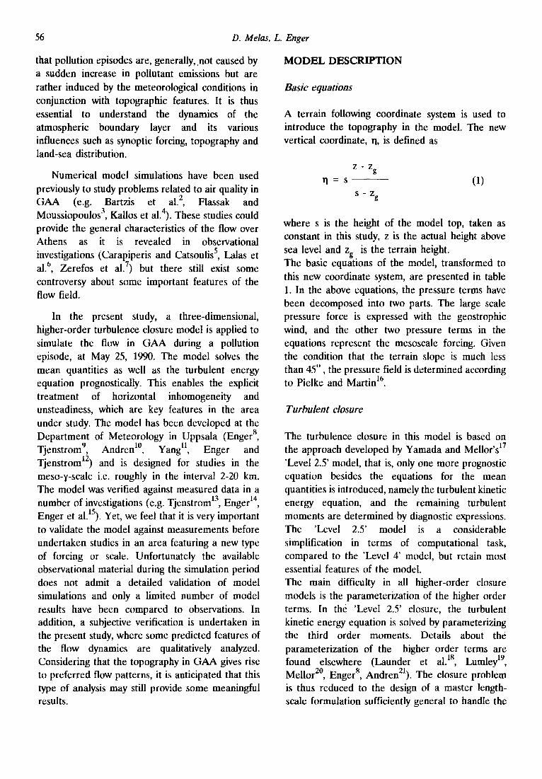
Athens basin is located on the west coast of the Attica peninsula (Fig. 1). The city of Athens is surrounded by moderately high mountains forming a channel with only one major opening toward the sea to the southwest. There are four main mountains, Mount Aigaleo to the west of the valley (with elevations up to 450 m), Hymetus to the east (1050 m), Pendeli to the north-east (1100) and Parnitha to the north-west (1400m). The mountains are acting as physical barriers with only small gaps between them. The most important is the channel

Figure I. Topographic map of Attica peninsula.


between Hymetus and Pendeli leading to the northeast coast of Attica peninsula which gives the Athens basin access to the Etesians, the system of persistent northerly winds which reduce the likelihood of prolonged pollution episodes. Multistorey buildings almost cover the floor of the valley for a distance of 20 km inland.

Details about the terrain height and the land use for the study area were provided by the coordinator of APSIS, Prof. N Moussiopoulos. The values of potential temperature at the lower boundary were prescribed according to the observations. The diurnal change of the potential temperature was represented by a sinusoidal wave which was fitted to temperature observations at Hellinikon airport. The potential temperature at the different gridpoints are furthermore supposed to be a function of height above sea level. In the present study it is assumed

O o = (9os - Zg /150 (3)

where (9os is the temperature at sea level. The temperature of the sea surface was set to 20°C.

In the horizontal a telescoping grid is employed, thc grid distance being 1 km in the central parts of the model. The total amount of grid points on each vertical level is 35 x 35, covering a horizontal domain with dimensions 80 x 100 km. At the onset of the integration there is no topography in the model during 4h of integration. As initial temperature profile we have used the measured profile according to the radiosonde measurements. As initial wind profile we have used the geostrophic wind estimated from the radiosonde measurements at 2.00 LST and below 150 m a logarithmic wind profile. The geostrophic wind speed was kept constant throughout the simulation period. This is found necessary because of the serious problems that might arise when the geostrophic wind varies with time. In that case, spurious inertial oscillations may occur in the model which tend to ruin the simulations.

it is considered that the temperature and the wind fields have come into some kind of balance with each other. After this initialization period the real simulation starts by changing the surface boundary conditions for potential temperature with time. The time step was chosen at 15s.

0 bservations

The only meteorological measurements available in this study are surface meteorological data that have been recorded at seven meteorological stations operating in GAA and upper air data from the radiosonde station at the airport of Athens.

The surface meteorological data obtained in the urban environment are expected to show local effects and should be interpreted with care.

ANALYSIS OF THE RESULTS

During the simulation day of the 25th of May, 1990, Greece was under the influence of a high pressure system which covered the east part of the Mediterranean. The pressure gradients were rather weak and the associated synoptic wind at 700 hPa was during night from the NW with speeds of -6.9 ms q. At 1400 LST the flow at 700 hPa was from the NNW and the wind speed decreased to about

-1 4.2 ms

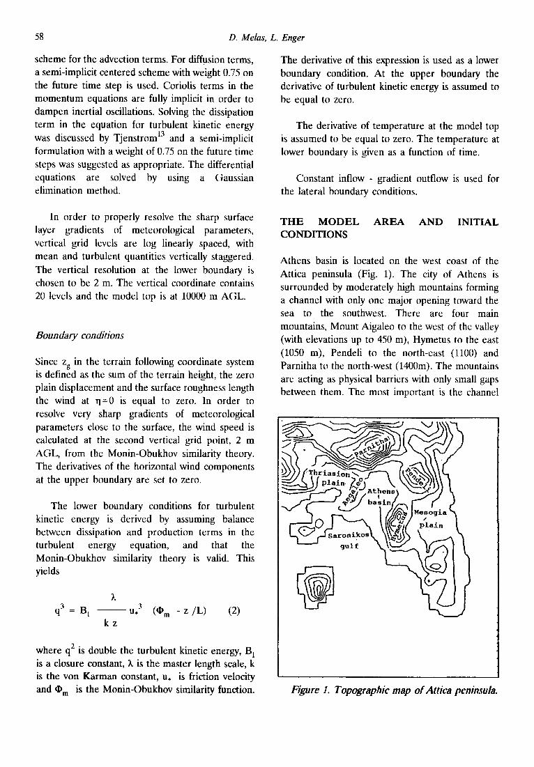
In figs 2a-d the simulated wind fields at 6.00, 9.00, 12.00 and 2100 LST are shown. The corresponding height is 25.4 m above the surface. The simulated wind fields are quite variable both in time as well as in space. At 6.00 local time, the flow is W over the sea, while the winds over Athens basin are light with variable directions (mostly from SW). Since the temperature of the land surface was slightly higher than the sea surface temperature, a land breeze circulation did not occur during this specific day. This was also confirmed by the observations at NOA which show light winds from S at 6.00 LST.

After this initial phase, we start the integration with the three-dimensional model and the terrain is allowed to grow linearly from zero to its final height. The model is run for 3 more hours before

During day-hours, the situation changes drastically. Thermally induced local circulations start to develop and the flow regime in GAA is more complicated. At 9.00 local time, the flow over the sea is generally


( km l

l O

1 J

20

I t

' i ' r ~ i i~ i ; i , , • • i . r r r i l . i . . . . . . . , , , • 1 , ~ t . l . , l ' r T l T r r l ' l r . . . . l . . . . . . .

, . ' . "1 " " " , " " ' ~ ' . ' , i " . • ! . . . . , q " . . . . ' . . - . " ' . . , ' , , , • . . . : ;

• " . ' / ; I " ' " . J ' - . . ; , . . - - !

, ! t . . .. -..,.. .. , . . . . . . .: , '1 i . l • . " * I , ' ~ l ~ ' ; ; " . . . . . . . " - ~ " . . . . . | ~ i • " . • * " " ' "'~ " , ," . ' . . ; ' ' ~ t .

• ," '| . . . . . . . . ' ..... ".,"~".'.t'.'." • I" " "

. . . . J ~ " i ' x i , .L : I . - / I l l I 0

• * l , i " "" ',,, . . . . . . . . . .~ .... ~ . . . . . . . . . . : 2 : : ~" : l . . . . . . , , : . . . . . . . . . . . . ~ . . . . . ~ . . . , . . , ~ . "

• . o , ~ , - , o * * * * * * * . ~ , . ~ o , o . o . o o • .- . . • ¢ , . , o , . . . 1 1 1 , , . - o . . . .

0 - • • • , . . . . . i . ' . . . , , , . . . r ~ . . . " : : . . . .

= . . . ' _ r . ' : : = . . . . . . r - - - .~ i - : . ' - ' - . - - ~ ; " ; : - " -

.,, : : ::::::::::::::::::i .... - I,: if: r . . . . ' i " I -- I ' - --C' ~ : ? k T il ~ i - - I !"

" : : : : : : : : . . . . . . . . "r. / r : / " .,, ; : , : / " "~ . . . . . . . . F - : - i"

f ~ r? 'F r~ tT ~ I 1 r | 1T I1 ' ' ' 1 . . . . I " ' ' ' 1 r '

- 3 0 -2J -10 - I ! - I 0 -$ 0 $ I 0 I S ~10 ~ 3 } 0 ( k i n )

( i t , . ) ,.-.v • i . . . . i . . . . r , . , " l . . . . i • .. - i a.p • • I - , ~ ~, i ,,, i • 1~ , • • i . . T r r r l r l ' l ~ r l ? l ~ r r f 4

~ - . . ~ ' - . - ~ - " ..' _ ~ - _ - . ~ i • . . . . . . . " i I ',

.... .tr. , : 7 : . • ;" ~- , . f . ,'2-. " . . , . . l o "~ ~ ~ . " ~ - ~ " . ~ ' - " ~ ' - ~ ' ) . ' . : "..'" . . . . . . , .... . ' - , - , - . . , ' . : . : , ~ . . . . . . . . , , , , ~.L . . . . . !

" . ; . . ' V / ? ; . ; ; ; . ; , ~ 3 2 o ; L , 2 . 3 , , - ' . . , .,.•.,,. , , - : T - / . ~ . . . . . . ~ , .% . . . . . . . ; . . - : t : - = " ~ t \ * :- • .

? -

: I . . . . . . - - : ' "_"__, - - ; . . - " . - ' - - ! - - - - q _ _ _ I L - ',. i l . . q - - - . - - - , ? ; . . . . . C ' , ' - ' - t - - ; -

] j _ - _ J ~ . . . . . . . . ~ v ' . : , . 2 , : ~ ' - ~ _ _ ! _ .,ot / ,,"',, ,.-. ° -- ' v " . ' . I

T -~'-r . . . . . . . . . . . . . . . . . . . ~ - - , - , - -"

.10 L t" i

..10 - l J -10 - IS - tO -5 0 $ I 0 15 ~ 2~t ~11 l i m p

( imp

I O

I t

i O

I I

t O

!

0 {

. 1 2

• tO 2

, I S

- 2 0

- l l

. 1 0

r l ' l I ' | I f i ' l | I r l ~ ' r r r y i i . ' , , , I , , . r l , , . . i , ~ , , i , , i , l l . , , l . y i , l . . . . i I , , , i , , • l

• : . :.~. :;-. ;-~,:..- L..~-AY\. L • • : ;, " <, , , . : : ;.:. ; " : . :~v , I Z ........ ; - / / / , ..__" -., ,,, ~ "" ~ r " . '7 ..-.-.:.,', ,,.'_2 ,(_,. ," ~---'-, _ J " > " " "',">:> "- ":~" .... -'" " i" "

I " ~' • . , - . - i . 7 , " , . . 7 : . ~ . - ; : ; . ; ' ; ~ . " \ ~

., , . " I . . . . . ; L . . . . . . . L. V" "'" ~ "v,~., ! ~ . u , ' " " " ' " ' - ; T r ~ " "

. . _ , . , . . . . . . . . . - . . . . . . . . . . . . ' - . ~ : ~ . - . : . r * .

. . . . . . - = - ~ :;:;L :iX_,-.'-'Z_.,2 212 ; - - - - ' ~ * ' - ~ . . ~ : ; ~ " " I /

j i " i : • / t

" l ~ ' r | ~ r l l ~ I v t i "1 r r ~ l I ' " " ' I . . . . i . . . . I ° ' ' ' l . . . . I . . . . l ' ' ' ' l / ' • ' f t ' ' '

. I f1 . l ~ .111 .1~ 40 .~ I I ~ tO iS IO 25 30 ( k i n )

( I nn )

30 -

2 0 -"

I - 5 - '

no 2

- 5 -

0 -

- I 0 -

-15 A

-20 -

-2~

-]0

, t . d • ~ . J / r . ~ \ ~ . '~ . ' I I .< ,-'x. . . . . , - . . e , ~ . , ~ . t J . . . . . . . . - , . - . / M / " I \ , ,.

PJ ~ ( . , - . , . - , .~-~.=. . , . ,e . . , .~. . l ( . :~-~, . .X,3 t .~ . . . . " J r ) . / ~ . . . . ~ . , J . ~ I ~t ",. \\'.\.'"\\ ~ "~ I

. . . . . . " : " ' , , . " - - ' _ ' r ~ ' r " r " " . . . . ~ -~ ~ " " - " " l ; t ' , ~ " ~ . . . . . . , ' " . , . ' ~ - ~ . ~ " r " "

--~ : : : : , - . ~ : : ' i : : : . . ~ ; : : , . . i ~ : . - ] ~ : . : .

............. -....%1 i.,,~.~:i~ . . . . . . . . ~. .

: ~ - 7 ~ : : . . . . . . . . ~,~,,~>;~<~- ; h " ~<.= ¢ - - . . . . : : : : : : : : ' - : , : ~ ~ ' : : " L " ~ ' V ' ~ I : ~- ~ : . . . . . . . ~. ~ . , ll<~.-".t I

r . . . . . . . . ~ ' ~ . . . . . . . . %." ~ - ' \ e < . . - r - " ! -

I . . , . ' . . . _ _ .

\ / 2 - L : 2c_:_;. :: {:- :- ,

.... i .... i .... I .... i .... i .... i.,•.i .... i .... i .... i .... i .... II'••i '.,

* l O - l ~ - 1 0 . I J - I 0 -~ 0 ~ I(1 1.5 I I I ~.~ I l l l i m p

Figure 2. Simulated wind 5elds at 25.4 rn A(.;L at (a) 6.00 LST, (b) 9.00 1.ST, (c) 12.00 LST, (d) 2t.OO LST.

from the W with speeds - 4 ms -1 but there is a splitting over Saronic gulf and part of the air moves over the Athens basin. This is due to the development of the sea breeze circulation which diverts part of the flow towards Athens basin. The winds over Athens area are coming from SW and they are rather light, 1-2 ms 1. This model prediction is in agreement with the observed winds over Athens area (Fig. 5 in Kallos et al.4). The notable wind deceleration downwind the shoreline is resulting from the high roughness of the city and has large consequences on pollutant dispersion in the area.

This is the only sea breeze circulation which can be readily identified from the simulated wind field• In the west side of mountain Aigaleo, at Thriassion plain, the flow is from the WSW and a probable explanation is that the sca-breeze merges with the prevailing flow and is difficult to distinguish. In the east part of Attica peninsula, at Mesogia plain, model results show that the flow is from W, thus prohibiting the development of a sea breeze circulation. This result is confirmed by observations at Spata airport which do not indicate the existence of a sea-breeze circulation in the area for the specific day (Fig. 5 in Kallos et al.4).

A numerical study offlow in Athens area using the MIUU model 61

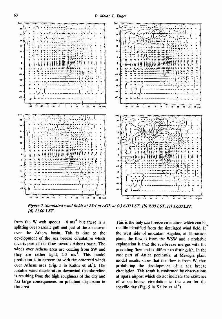
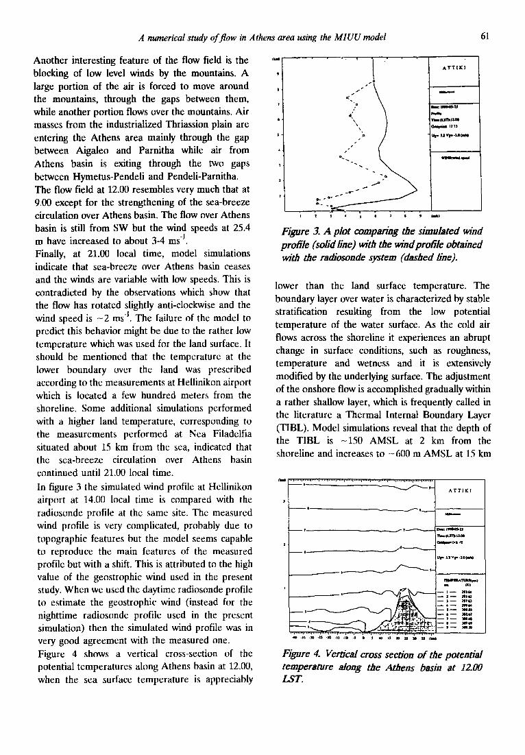
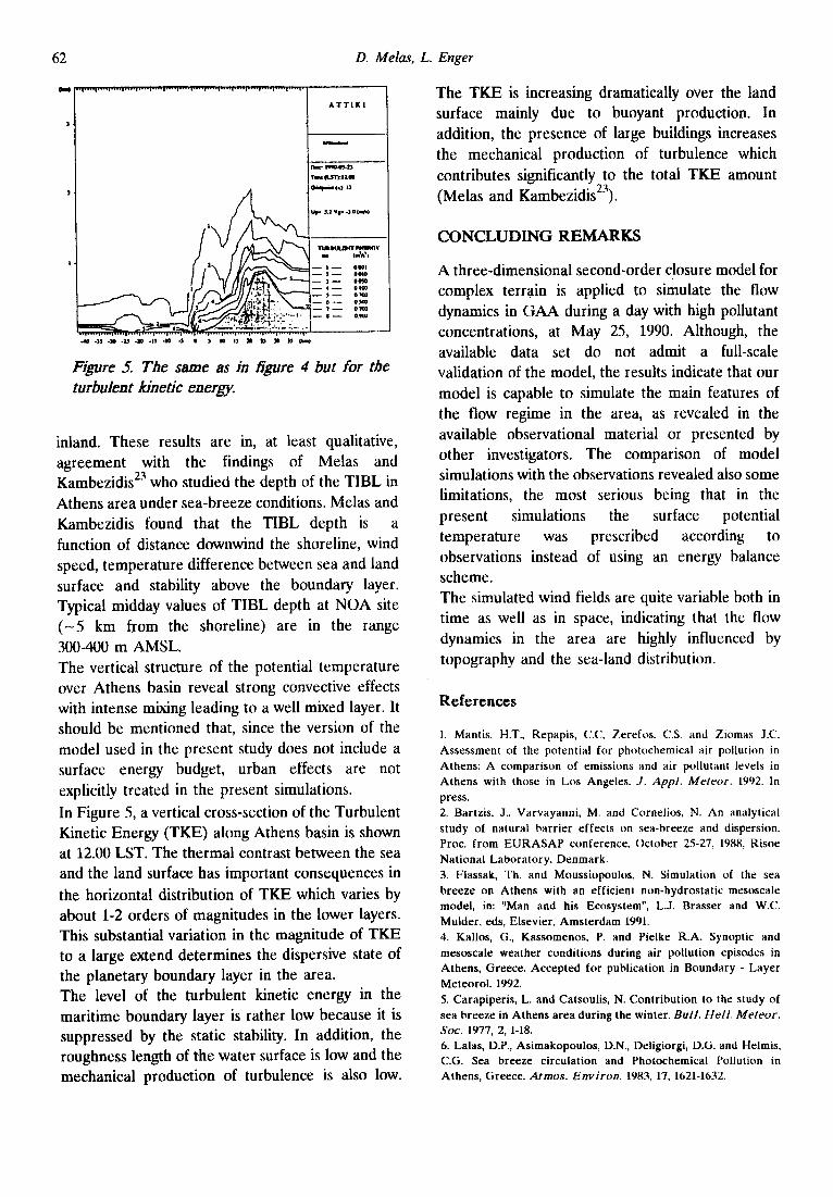
Another interesting feature of the flow field is the blocking of low level winds by the mountains. A large portion of the air is forced to move around the mountains, through the gaps between them, while another portion flows over the mountains. Air masses from the industrialized Thriassion plain are entering the Athens area mainly through the gap between Aigaleo and Parnitha while air from Athens basin is exiting through the two gaps between Hymetus-Pendeli and Pendeli-Parnitha. The flow field at 12.00 resembles very much that at 9.00 except for the strengthening of the sea-breeze circulation over Athens basin. The flow over Athens basin is still from SW but the wind speeds at 25.4 m have increased to about 3-4 ms -l. Finally, at 21.00 local time, model simulations indicate that sea-breeze over Athens basin ceases and the winds are variable with low speeds. This is contradicted by the observations which show that the flow has rotated slightly anti-clockwise and the wind speed is N 2 ms -l. The failure of the model to predict this behavior might be due to the rather low temperature which was used for the land surface. It should be mentioned that the temperature at the lower boundary over the land was prescribed according to the measurements at Hellinikon airport which is located a few hundred meters from the shoreline. Some additional simulations performed with a higher land temperature, corresponding to the measurements performed at Nea Filadelfia situated about 15 km from the sea, indicated that the sea-breeze circulation over Athens basin continued until 21.00 local time. In figure 3 the simulated wind profile at HeUinikon airport at 14.00 local time is compared with the radiosonde profile at the same site. The measured wind profile is very complicated, probably due to topographic features but the model seems capable to reproduce the main features of the measured profile but with a shift. This is attributed to the high value of the geostrophic wind used in the present study. When we used the daytime radiosonde profile to estimate the geostrophic wind (instead for the nighttime radiosonde profile used in the present simulation) then the simulated wind profile was in very good agreement with the measured one. Figure 4 shows a vertical cross-section of the potential temperatures along Athens basin at 12.00, when the sea surface temperature is appreciably

IlVml

9

I .

T

5 '

4

A T T [ K I

k ~

1711

O r U V p - ~

Figure 3. A plot comparing the simulated wind profile (soh'd h'ne) with the wind profile obtained with the ra~'osonde system (dashed line).

lower than the land surface temperature. The boundary layer over water is characterized by stable stratification resulting from the low potential temperature of the water surface. As the cold air flows across the shoreline it experiences an abrupt change in surface conditions, such as roughness, temperature and wetness and it is extensively modified by the underlying surface. The adjustment of the onshore flow is accomplished gradually within a rather shallow layer, which is frequently called in the literature a Thermal Internal Boundary Layer (TIBL). Model simulations reveal that the depth of the TIBL is -150 AMSL at 2 km from the shoreline and increases to -600 m AMSL at 15 km

~ ' ' 1 . ` ' ' ~ ' ' 1 ' ' . - r - ' . ` v -~ . ` 1" . - ` v '~ - . 1 ' ' . ' 1 - ' ' ' ~ - ' ' - l ' ' - ' r ' ' - . ~ * ' ' - ~ ' ' ' ~1" . ' ' ' r ~ - " I ,

)

I , , ,

7

It

t - - j 6 - . . - - . . . - - . . . . . _ _ . _ _

/ ~ ' - - - % - 5-

A T T I K I

u p ~,1 v p -lOte~l

I 'rbl;11u~'ralm@~l Oil

' _ _ - - I - ~ I . I I - - ~S61

3 - - ~ M I 6 - - IOll~

I - - =- ,-:-- "'-.'" -15 .lid .U .ID . i j .HI . i I J I0 i I I l l ]~ ] l !.5 (1111~

Figure 4. Vertical cross section of the potential temperature along the Athens basin at 12.00 LST.


)

I

S~

ATT IK I

T R ¢ J ' ~ IZIO

U w. $.| Vp .)@lai~}

- - I - o w l - - 2 - OO~ - - 3 - - 0 0 ~ 0

- - ~ J - - Ooao

- - 6 - - 0 5 0 ~ - - ~ - - 03qO0

- - $ - - O.5m

• ~ -35 .N .ZS 40 - I J . t o -5 • 3 t o t , I o ~ l o I~ Ibm)

Figure 5. The same as in tigure 4 but for the turbulent kinetic energy.

inland. These results are in, at least qualitative, agreement with the findings of Melas and Kambezidis 23 who studied the depth of the TIBL in Athens area under sea-breeze conditions. Melas and Kambezidis found that the TIBL depth is a function of distance downwind the shoreline, wind speed, temperature difference between sea and land surface and stability above the boundary layer. Typical midday values of TIBL depth at NOA site (N5 km from the shoreline) are in the range 300-400 m AMSL. The vertical structure of the potential temperature over Athens basin reveal strong convective effects with intense mixing leading to a well mixed layer. It should be mentioned that, since the version of the model used in the present study does not include a surface energy budget, urban effects are not explicitly treated in the present simulations. In Figure 5, a vertical cross-section of the Turbulent Kinetic Energy (TKE) along Athens basin is shown at 12.00 LST. The thermal contrast between the sea and the land surface has important consequences in the horizontal distribution of TKE which varies by about 1-2 orders of magnitudes in the lower layers. This substantial variation in the magnitude of TKE to a large extend determines the dispersive state of the planetary boundary layer in the area. The level of the turbulent kinetic energy in the maritime boundary layer is rather low because it is suppressed by the static stability. In addition, the roughness length of the water surface is low and the mechanical production of turbulence is also low.

The TKE is increasing dramatically over the land surface mainly due to buoyant production. In addition, the presence of large buildings increases the mechanical production of turbulence which contributes significantly to the total TKE amount (Melas and Kambezidis23).

CONCLUDING REMARKS

A three-dimensional second-order closure model for complex terrain is applied to simulate the flow dynamics in GAA during a day with high pollutant concentrations, at May 25, 1990. Although, the available data set do not admit a full-scale validation of the model, the results indicate that our model is capable to simulate the main features of the flow regime in the area, as revealed in the available observational material or presented by other investigators. The comparison of model simulations with the observations revealed also some limitations, the most serious being that in the present simulations the surface potential temperature was prescribed according to observations instead of using an energy balance scheme. The simulated wind fields arc quite variable both in time as well as in space, indicating that the flow dynamics in the area are highly influenced by topography and the sea-land distribution.

References

1. Mantis, H.T., Repapis, C.C, Zerefos. C.S. and Ziomas J.C'. Assessment of the potential for photochemical air pollution in Athens: A comparison of emissions and air pollutant levels in Athens with those in Los Angeles. J. Appl. Meteor. 1992. In press. 2. Bartzis. J., Varvayanni, M. and Cornelios, N. An analytical study of natural barrier effects on sea-breeze and dispersion. Proc. from EURASAP conference. October 25-27, 1988, Risoe National Laboratory. Denmark. 3. Flassak, Th. and Moussiopoulos, N. Simulation of the sea breeze on Athens with an efficient non-hydrostatic mesoscale model, in: 'JMan and his Ecosystem", L.J. Brasser and W.C. Mulder, eds, Elsevier. Amsterdam 1991. 4. Kallos, G., Kassomenos, P. and Pielke R.A. Synoptic and mesoscale weather conditions during air pollution episodes in Athens, Greece. Accepted for publication in Boundary - Layer Meteorol. 1992. 5. Carapiperis, L. and Catsoulis, N. Contribution to the study of sea breeze in Athens area during the winter. Bull. Hell. Meteor. Soc. 1977, 2, 1-18. 6. Lalas, D.P., Asimakopouios, D.N., Deligiorgi, D.G. and Helmis, C.G. Sea breeze circulation and Photochemical Pollution in Athens, Greece. Atmos. Environ. 1983, 17, 1621-1632.


7. Zerefos, C., Ziomas, I., Bais, A., Mantis, H., Repapis, C., Amanatidis, G., Paliatsos, A. and Roemer, G. Development of air pollution levels in the Athens basin, Report to the Greek Ministry of Environment, Land use and Public Works. Athens 1989 (in Greek). 8. Enger. L. A higher order closure model applied to dispersion in a convective PBL. Atmos. Environ. 1986, 20. 879-894. 9. Tjenstrom, M. Numerical simulation of stratiform boundary layer clouds on the meso-'t-scale. Part 1: The influence of terrain height differences. Boundary-Layer Meteorol. 1988. 44,

207-230. 10. Andren, A. A TKE-dissipation model for the atmospheric bounadary layer. Boundary-Layer Meteorol. 1991, 56, 207-221. 11. Yang, X. A study of nonhydrostatic effects in idealized sea breeze systems. Boundary-Layer Meteor. 1991, 54, 183-208. 12. Enger, L. and Tjenstrom, M. Estimating the effect on the regional precipitation climate in a semi-arid region caused by an artificial lake using a mesoscale model. J. Appl. Meteor. 1991.30,

227-250. 13. Tjenstrom, M. A study of flow over complex terrain using a three dimensional model. A preliminary model evaluation focusing on stratus and fog. Annales Oeophysicae 1987, 5B. 4~)9-486. 14. Enger. L. Simulation of dispersion in moderately complex terrain-Part A. The fluid dynamic model. Atmos. Environ. 1991, 24. 2431-2446.

15. Enger, L., Koracin, D. and Yang, X. A numerical study of the boundary layer in complex terrain. Part 1. Sensitivity tests of boundary conditions and external forcing. Accepted for publication in Boundary-Layer Meteorology 1992. 16. Pielke. R.A. and Martin, C.L. The derivation of a terrain following coordinate system for use in a hydrostatic model. J. Atmos. Sci. 1981, 38, 1707-1713. 17. Yamada, T. and Mellor, G.L A simulation of the Wangara atmospheric boundary layer data . . I . Atmos. Sci. 1975, 32,

2309-2329.

18. Launder, G., Reece, J. and Rodi, W. Progress in the development of a Reynolds stress turbulent closure. J. F lu id

Mech. 1975. 68, 537-566. 19. Lumley, J.L. Computational modeling of turbulent flows. Adv. Appl. Sci. 1979, 18, 123-176. 20. Mellor, G.L. Analytic prediction of the properties of stratified planetary surface layers. J. Atmos. Sci. 1973, 30, 1061-1069. 21. Andren, A. Evaluation of a turbulence closure scheme suitable for air-pollution applications. J. Appl. Meteor. 1990, 29, 224-239. 22. Enger, L. A three-dimensional time dependent model for the meso-7-scale - some test results with a preliminary version. Report No 80. Department of Meteorology. Uppsala tTniversily, Uppsala. Sweden 1984. 23. Melas, D. and Kambezidis H. D. The depth of the internal boundary layer at an urban area under sea breeze conditions. Boundary - Layer Meteorol . 1992, 61, 247-264.

Documents

A numerical study of floe in Athens area using the MIUU model