Embed Size (px)
Citation preview
A Novel Linear Polarization Resistance Corrosion Sensing Methodologyfor Aircraft Structure
Douglas W. Brown1, Richard J. Connolly2, Bernard Laskowski3, Margaret Garvan4, Honglei Li5, Vinod S. Agarwala6, andGeorge Vachtsevanos7
1,2,3 Analatom, Inc., 3210 Scott Blvd., Santa Clara, CA 95054, [email protected]
[email protected]@analatom.com
4,5,7 Department of Electrical and Computer Engineering, Georgia Institute of Technology, Atlanta, GA 30332, [email protected]@gatech.edu
6 Iron Pillar Technical Services, 1600 Green Street, Philadelphia, PA 19130, [email protected]
ABSTRACT
A direct method of measuring corrosion on a structure us-ing a micro-linear polarization resistance (µLPR) sensor ispresented. The new three-electrode µLPR sensor design pre-sented in this paper improves on existing LPR sensor tech-nology by using the structure as part of the sensor system,allowing the sensor electrodes to be made from a corro-sion resistant or inert metal. This is in contrast to a two-electrode µLPR sensor where the electrodes are made fromthe same material as the structure. A controlled experiment,conducted using an ASTM B117 salt fog, demonstrated thethree-electrode µLPR sensors have a longer lifetime and bet-ter performance when compared to the two-electrode µLPRsensors. Following this evaluation, a controlled experimentusing the ASTM G85 Annex 5 standard was performed toevaluate the accuracy and precision of the three-electrodeµLPR sensor when placed between lap joint specimens madefrom AA7075-T6. The corrosion computed from the µLPRsensors agreed with the coupon mass loss to within a 95%confidence interval. Following the experiment, the surfacemorphology of each lap joint was determined using laser mi-croscopy and stylus-based profilometry to obtain local andglobal surface images of the test panels. Image processing,feature extraction, and selection tools were then employed toidentify the corrosion mechanism (e.g. pitting, intergranular).
Douglas Brown et al. This is an open-access article distributed under theterms of the Creative Commons Attribution 3.0 United States License, whichpermits unrestricted use, distribution, and reproduction in any medium, pro-vided the original author and source are credited.
1. INTRODUCTION
Recent studies have exposed the generally poor state of ournation’s critical infrastructure that has resulted from wearand tear under excessive operational loads and environmen-tal conditions. The British Standards Institution’s PubliclyAvailable Specification for the optimized management ofphysical assets defines asset management as the “systematicand coordinated activities and practices through which an or-ganization optimally and sustainably manages its assets andasset systems, their associated performance, risks and expen-ditures over their life cycles for the purpose of achievingits organizational strategic plan.” The motivation for effec-tive asset management is driven by owners’ desire for highervalue assets at less overall costs, thus extracting the maximumvalue from their assets (Herder & Wijnia, 2011). Condition-based maintenance aims to maximize asset value by extend-ing the useful life of assets through mitigation of unnecessarymaintenance actions performed during schedule-based main-tenance strategies (Huston, 2010). By providing maintenanceengineers with information regarding the health of the struc-ture, maintenance can be performed on a basis of necessityunique to each asset, as opposed to schedule-based predic-tions formed on statistical trends of operational reliability.These systems must be low-cost and simple to install witha user interface designed to be easy to operate.
To reduce the cost and complexity of such a system for mon-itoring corrosion in an avionics environment, a generic inter-face node using low-powered wireless communications has
1
ANNUAL CONFERENCE OF THE PROGNOSTICS AND HEALTH MANAGEMENT SOCIETY 2014
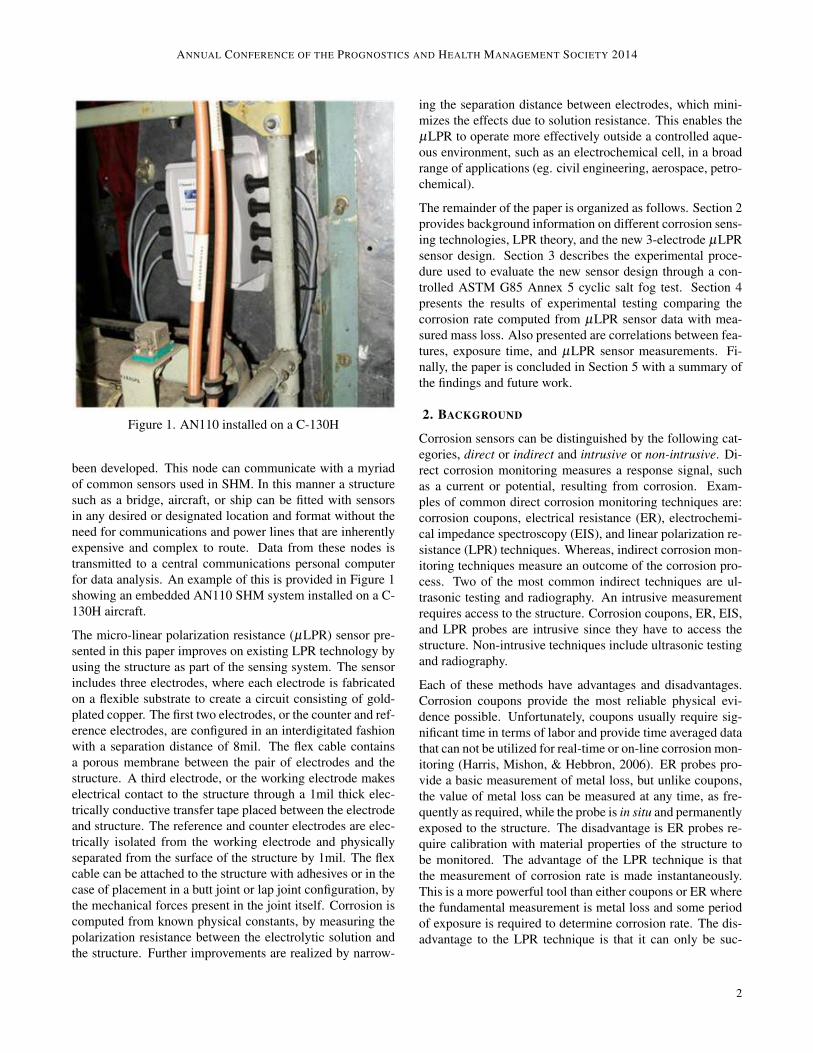
Figure 1. AN110 installed on a C-130H
been developed. This node can communicate with a myriadof common sensors used in SHM. In this manner a structuresuch as a bridge, aircraft, or ship can be fitted with sensorsin any desired or designated location and format without theneed for communications and power lines that are inherentlyexpensive and complex to route. Data from these nodes istransmitted to a central communications personal computerfor data analysis. An example of this is provided in Figure 1showing an embedded AN110 SHM system installed on a C-130H aircraft.
The micro-linear polarization resistance (µLPR) sensor pre-sented in this paper improves on existing LPR technology byusing the structure as part of the sensing system. The sensorincludes three electrodes, where each electrode is fabricatedon a flexible substrate to create a circuit consisting of gold-plated copper. The first two electrodes, or the counter and ref-erence electrodes, are configured in an interdigitated fashionwith a separation distance of 8mil. The flex cable containsa porous membrane between the pair of electrodes and thestructure. A third electrode, or the working electrode makeselectrical contact to the structure through a 1mil thick elec-trically conductive transfer tape placed between the electrodeand structure. The reference and counter electrodes are elec-trically isolated from the working electrode and physicallyseparated from the surface of the structure by 1mil. The flexcable can be attached to the structure with adhesives or in thecase of placement in a butt joint or lap joint configuration, bythe mechanical forces present in the joint itself. Corrosion iscomputed from known physical constants, by measuring thepolarization resistance between the electrolytic solution andthe structure. Further improvements are realized by narrow-
ing the separation distance between electrodes, which mini-mizes the effects due to solution resistance. This enables theµLPR to operate more effectively outside a controlled aque-ous environment, such as an electrochemical cell, in a broadrange of applications (eg. civil engineering, aerospace, petro-chemical).
The remainder of the paper is organized as follows. Section 2provides background information on different corrosion sens-ing technologies, LPR theory, and the new 3-electrode µLPRsensor design. Section 3 describes the experimental proce-dure used to evaluate the new sensor design through a con-trolled ASTM G85 Annex 5 cyclic salt fog test. Section 4presents the results of experimental testing comparing thecorrosion rate computed from µLPR sensor data with mea-sured mass loss. Also presented are correlations between fea-tures, exposure time, and µLPR sensor measurements. Fi-nally, the paper is concluded in Section 5 with a summary ofthe findings and future work.
2. BACKGROUND
Corrosion sensors can be distinguished by the following cat-egories, direct or indirect and intrusive or non-intrusive. Di-rect corrosion monitoring measures a response signal, suchas a current or potential, resulting from corrosion. Exam-ples of common direct corrosion monitoring techniques are:corrosion coupons, electrical resistance (ER), electrochemi-cal impedance spectroscopy (EIS), and linear polarization re-sistance (LPR) techniques. Whereas, indirect corrosion mon-itoring techniques measure an outcome of the corrosion pro-cess. Two of the most common indirect techniques are ul-trasonic testing and radiography. An intrusive measurementrequires access to the structure. Corrosion coupons, ER, EIS,and LPR probes are intrusive since they have to access thestructure. Non-intrusive techniques include ultrasonic testingand radiography.
Each of these methods have advantages and disadvantages.Corrosion coupons provide the most reliable physical evi-dence possible. Unfortunately, coupons usually require sig-nificant time in terms of labor and provide time averaged datathat can not be utilized for real-time or on-line corrosion mon-itoring (Harris, Mishon, & Hebbron, 2006). ER probes pro-vide a basic measurement of metal loss, but unlike coupons,the value of metal loss can be measured at any time, as fre-quently as required, while the probe is in situ and permanentlyexposed to the structure. The disadvantage is ER probes re-quire calibration with material properties of the structure tobe monitored. The advantage of the LPR technique is thatthe measurement of corrosion rate is made instantaneously.This is a more powerful tool than either coupons or ER wherethe fundamental measurement is metal loss and some periodof exposure is required to determine corrosion rate. The dis-advantage to the LPR technique is that it can only be suc-
2
ANNUAL CONFERENCE OF THE PROGNOSTICS AND HEALTH MANAGEMENT SOCIETY 2014
cessfully performed in relatively clean aqueous electrolyticenvironments (Introduction to Corrosion Monitoring, 2012).EIS is a very powerful technique that can provide a corrosionrate and classification of the corrosion mechanism. EIS mea-sures the magnitude and phase response of an electrochemicalcell. Physical parameters, such as the polarization resistance,solution resistance, and double-layer capacitance, can be de-rived from these responses, which provides more informationthan just LPR alone. The disadvantage with EIS is that ituses sophisticated instrumentation that requires a controlledsetting to obtain an accurate spectrum. In fielded environ-ments, EIS is highly susceptible to noise. Additionally, in-terpretation of the data can be difficult (Buchheit, Hinkebein,Maestas, & Montes, 1998). Ultrasonic testing and radiog-raphy can be used to detect and measure (depth) corrosionthrough non-destructive and non-intrusive means (Twomey,1997). The disadvantage with the ultrasonic testing and ra-diography equipment is the same with corrosion coupons,both require significant time in terms of labor and can notbe utilized for real-time or on-line corrosion monitoring. Asthis paper is focused on a three-electrode µLPR sensor, theremainder of the background will focus on LPR.
2.1. LPR Theory
Corrosion occurs as a result of oxidation and reduction re-actions occurring at the interface of a metal and an elec-trolyte solution. This process occurs by electrochemical half-reactions; (1) anodic (oxidation) reactions involving dissolu-tion of metals in the electrolyte and release of electrons, and(2) cathodic (reduction) reactions involving gain of electronsby the electrolyte species like atmospheric oxygen, O2, H2O,or H+ ions in an acid (Harris et al., 2006). The flow of elec-trons from the anodic reaction sites to the cathodic reactionsites creates a corrosion current. The electrochemically gen-erated corrosion current can be very small (on the order ofnanoamperes) and difficult to measure directly. Applicationof an external potential exponentially increases the anodicand cathodic currents, which allows instantaneous corrosionrates to be extracted from the polarization curve. Extrapo-lation of these polarization curves to their linear region pro-vides an indirect measure of the corrosion current, which isthen used to calculate the rate of corrosion (Burstein, 2005).
The electrochemical technique of LPR is used to study corro-sion processes since the corrosion reactions are electrochem-ical reactions occurring on the metal surface. Modern cor-rosion studies are based on the concept of mixed potentialtheory postulated by Wagner and Traud, which states that thenet corrosion reaction is the sum of independently occurringoxidation and reduction reactions (Wagner & Traud, 1938).For the case of metallic corrosion in presence of an aqueousmedium, the corrosion process can be written as,
M+ zH2Of↔b
Mz++z2
H2 + zOH−, (1)
where z is the number of electrons lost per atom of the metal.This reaction is the result of an anodic (oxidation) reaction,
Mf↔b
Mz++ ze−, (2)
and a cathodic (reduction) reaction,
zH2O+ ze−f↔b
z2
H2 + zOH−. (3)
It is assumed that the anodic and cathodic reactions occur at anumber of sites on a metal surface and that these sites changein a dynamic statistical distribution with respect to locationand time (Kossowsky, 1989). Thus, during corrosion of ametal surface, metal ions are formed at anodic sites with theloss of electrons and these electrons are then consumed bywater molecules to form hydrogen molecules. The interac-tion between the anodic and cathodic sites as described on thebasis of mixed potential theory is represented by well-knownrelationships using current (reaction rate) and potential (driv-ing force). For the above pair of electrochemical reactions (2)and (3), the relationship between the applied current Ia andapplied potential, Ea, follows the Butler-Volmer equation,
Ia = Icorr
[e2.303(Ea−Ecorr)/βa − e−2.303(Ea−Ecorr)/βc
], (4)
where βa and βc are the anodic and cathodic Tafel parametersgiven by the slopes of the polarization curves ∂Ea/∂ log10 Iain the anodic and cathodic Tafel regimes, respectively andEcorr is the corrosion, or open circuit potential (Bockris,Reddy, & Gambola-Aldeco, 2000). The corrosion current,Icorr, cannot be measured directly. However, a priori knowl-edge of βa and βc along with a small signal analysis tech-nique, known as polarization resistance, can be used to in-directly compute Icorr. The polarization resistance technique,also referred to as linear polarization, is an experimental elec-trochemical technique that estimates the small signal changesin Ia when Ea is perturbed by Ecorr ± 10mV (G102, 1994).The slope of the resulting curve over this range is the polar-ization resistance,
Rp ,∂Ea
∂ Ia
∣∣∣∣|Ea−Ecorr |≤10mV
. (5)
ASTM standard G59 outlines procedures for measuring po-larization resistance. Potentiodynamic, potential step, andcurrent-step methods can be used to compute Rp (G59, 1994).The potentiodynamic sweep method is the most commonmethod for measuring Rp. A potentiodynamic sweep is con-ducted by applying Ea between Ecorr±10mV at a slow scanrate, typically 0.125 mV/s. A linear fit of the resulting Ea vs.Ia curve is used to compute Rp. Note, the applied current, Ia,is the total applied current and is not multiplied by the elec-trode area so Rp as defined in (5) has units of Ω. Provided that|Ea−Ecorr|/βa 1 and |Ea−Ecorr|/βc 1, the first order
3
ANNUAL CONFERENCE OF THE PROGNOSTICS AND HEALTH MANAGEMENT SOCIETY 2014
(a) (b)
(c) (d)
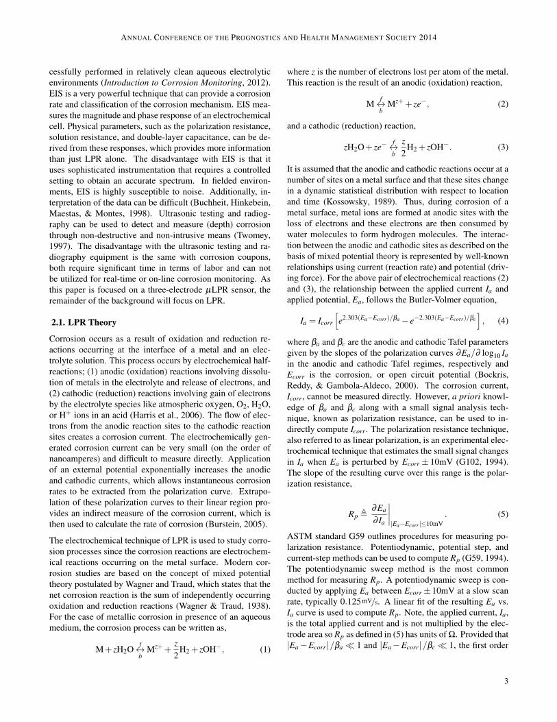
Figure 2. The (a) two-electrode µLPR sensor, (b) three-electrode µLPR sensor, (c) two-electrode µLPR sensor identifyingeach sensor element when mounted to a substrate, and (d) three-electrode µLPR sensor identifying each sensor element whenattached using the structure as the third electrode.
Taylor series expansion ex u 1+ x can be applied to (4) and(5) to arrive at the Stern-Geary equation,
Icorr =B?
Rp, (6)
where,
B? =βaβc
2.303(βa +βc). (7)
Knowledge of Rp, βa, and βc enables direct determination ofIcorr at any instant in time. The corrosion rate, Rloss, can befound by applying Faraday’s law,
Rloss (t) =Bloss
Rp (t), (8)
where,
Bloss =B?
FAsen
(AW
z
), (9)
such that F is Faraday’s constant, z is the number of electronslost per atom of the metal during an oxidation reaction, Asenis the effective area of the sensor, and AW is atomic weight.The total mass loss, Mloss, due to corrosion can be found byintegrating (8),
Mloss (t) =ˆ t
t0Rloss (τ)dτ. (10)
Finally, since Rp is not measured continuously (10) needs tobe discretized for the sample period Ts,
Mloss (t)∣∣∣∣t=NTs
= Ts
N
∑k=1
Rloss (kTs) . (11)
2.2. Sensor Design
The two-electrode µLPR design consists of a sensor withinterdigitated electrodes photo-etched from 2mil aluminumshim-stock material with a thickness and separation distance
of 12mil. In this configuration one of the electrode pairs actsas the counter electrode (cathode) and the other as the work-ing electrode (anode). The sensor is designed to corrode inthe same environment as the structure, effectively measuringthe corrosivity of the environment. An image of the two-electrode µLPR sensor is provided in Figure 2(a). An illus-tration showing the two-electrode µLPR sensor mounted tothe structure is shown in Figure 2(c).
Improving on the two-electrode design, the three-electrodeµLPR is fabricated on a flexible Kapton substrate where eachelectrode is coated with a noble metal. The first two elec-trodes, counter and reference electrodes, are fabricated us-ing 0.5 oz. copper with an electroless nickel immersion gold(ENIG) finish and an overall thickness of 1mil. The counterand reference electrode pair is configured in a interdigitatedgeometric layout with a separation distance of 9mil. The flexcable contains an insulating porous scrim material betweenthe pair of electrodes and the structure. A third electrode,made from the same ENIG finish, is placed in close proxim-ity to the counter and reference electrodes; electrical contactis made with the structure by placing a 1mil thick electricallyconductive transfer tape between the electrode and structure.This allows the structure to serve as the working electrodefor the sensor measurement. The flex cable, shown in Fig-ures 2(b) and (d), can be attached to the structure through theuse of adhesives or in the case of placement in a butt joint orlap joint configuration, the holding force is provided by thejoint itself.
3. EXPERIMENTAL PROCEDURES
3.1. Tafel Measurements
ASTM standard G59 outlines the procedure for measuringthe Tafel slopes, βa and βc. First, Ecorr is measured fromthe open circuit potential. Next, Ea is initialized to E corr-250mV. Then, a potentiodynamic sweep is conducted by in-creasing Ea from Ecorr−250mV to Ecorr +250mV at a slow
4
ANNUAL CONFERENCE OF THE PROGNOSTICS AND HEALTH MANAGEMENT SOCIETY 2014
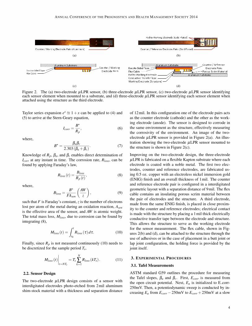
Figure 3. AA7075-T6 lap joint assembly.
scan rate, typically 0.125 mV/s. Finally, a Tafel curve is plot-ted for Ea vs. log10 Ia. Values for βa and βc are estimatedfrom the slopes of the linear extrapolated anodic and cathodiccurrents.
3.2. Sample Preparation
Lap joint samples were made using two 6” by 3” panels madefrom AA7075-T6 with a thickness of 1/8”. These panels weresecured together with six polycarbonate fasteners. Before as-sembly of the lap joint each panel was cleaned with a 35 minimmersion into a constantly stirred solution of 50 g/L Turco4215 NC-LT at 65C. After completing this alkaline cleaningthe panels were rinsed with deionized water and immersedinto a 70% solution of nitric acid solution for 5min at 25C.The samples were then rinsed again in the deionized waterand air dried. Weights were recorded to the nearest fifthsignificant figure and the samples were stored in a desicca-tor. Once the panels were prepared and massed, two µLPRsensors were installed between the panels. At this point thesix polycarbonate bolts were torqued down evenly to 2N ·m.This lap joint assembly is shown in Figure 3. After assem-bling the lap joints, the samples were evenly coated with 2mils of epoxy-based paint and 2 mils of polyurethane on allexposed surfaces. These coatings were allowed to fully sealover a 24 hour period at 35C before testing.
3.3. Comparing Two vs. Three Electrode Design
A preliminary experiment was performed to highlight thebenefits between a two-electrode µLPR sensor made fromAA7075-T6 and a three-electrode µLPR sensor made fromnickel. This experiment was performed by placing four two-electrode µLPR and four three electrode µLPR sensors into abeaker filled with a B117 salt solution modified to a pH of 5.5.A stirbar was used to constantly mix the solution. The sensorswere placed inside the beaker around a plastic cylindrical fix-ture. The two and three-electrode µLPR sensors were evenlyspaced in an alternating arrangement. Approximately every4 days, the coupons were removed, cleaned, massed and then
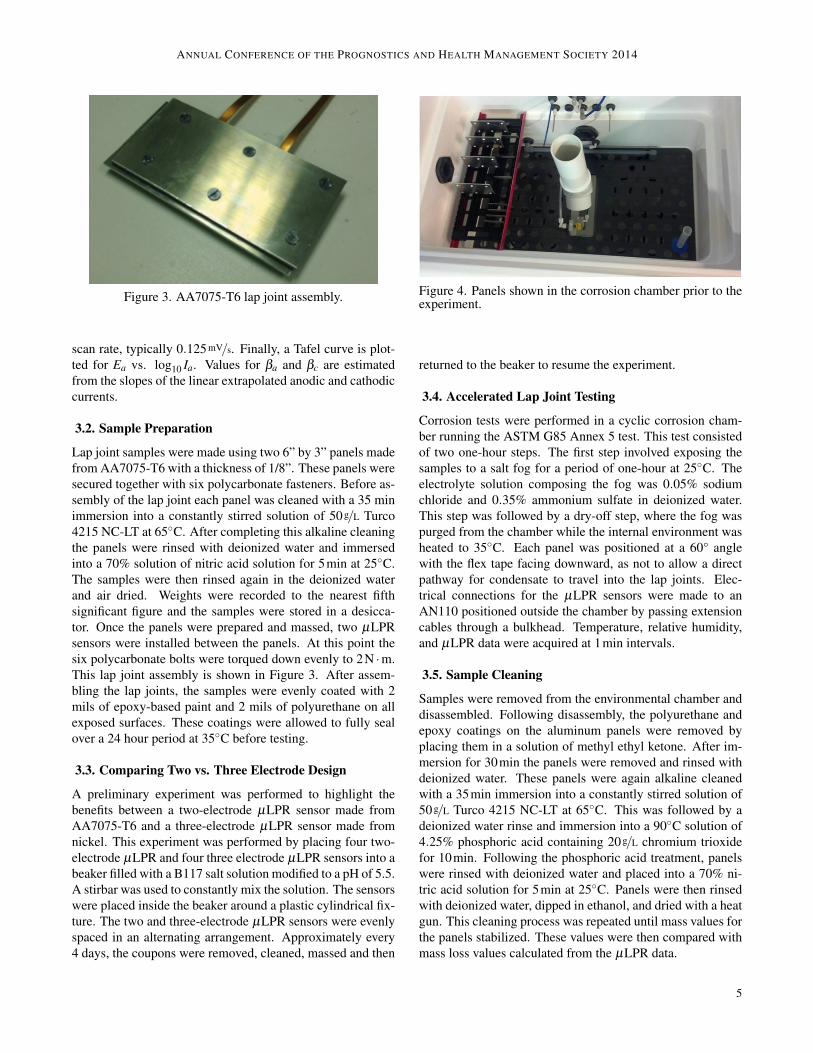
Figure 4. Panels shown in the corrosion chamber prior to theexperiment.
returned to the beaker to resume the experiment.
3.4. Accelerated Lap Joint Testing
Corrosion tests were performed in a cyclic corrosion cham-ber running the ASTM G85 Annex 5 test. This test consistedof two one-hour steps. The first step involved exposing thesamples to a salt fog for a period of one-hour at 25C. Theelectrolyte solution composing the fog was 0.05% sodiumchloride and 0.35% ammonium sulfate in deionized water.This step was followed by a dry-off step, where the fog waspurged from the chamber while the internal environment washeated to 35C. Each panel was positioned at a 60° anglewith the flex tape facing downward, as not to allow a directpathway for condensate to travel into the lap joints. Elec-trical connections for the µLPR sensors were made to anAN110 positioned outside the chamber by passing extensioncables through a bulkhead. Temperature, relative humidity,and µLPR data were acquired at 1min intervals.
3.5. Sample Cleaning
Samples were removed from the environmental chamber anddisassembled. Following disassembly, the polyurethane andepoxy coatings on the aluminum panels were removed byplacing them in a solution of methyl ethyl ketone. After im-mersion for 30min the panels were removed and rinsed withdeionized water. These panels were again alkaline cleanedwith a 35min immersion into a constantly stirred solution of50 g/L Turco 4215 NC-LT at 65C. This was followed by adeionized water rinse and immersion into a 90C solution of4.25% phosphoric acid containing 20 g/L chromium trioxidefor 10min. Following the phosphoric acid treatment, panelswere rinsed with deionized water and placed into a 70% ni-tric acid solution for 5min at 25C. Panels were then rinsedwith deionized water, dipped in ethanol, and dried with a heatgun. This cleaning process was repeated until mass values forthe panels stabilized. These values were then compared withmass loss values calculated from the µLPR data.
5
ANNUAL CONFERENCE OF THE PROGNOSTICS AND HEALTH MANAGEMENT SOCIETY 2014
4. RESULTS
4.1. Comparing Two vs. Three Electrode Design
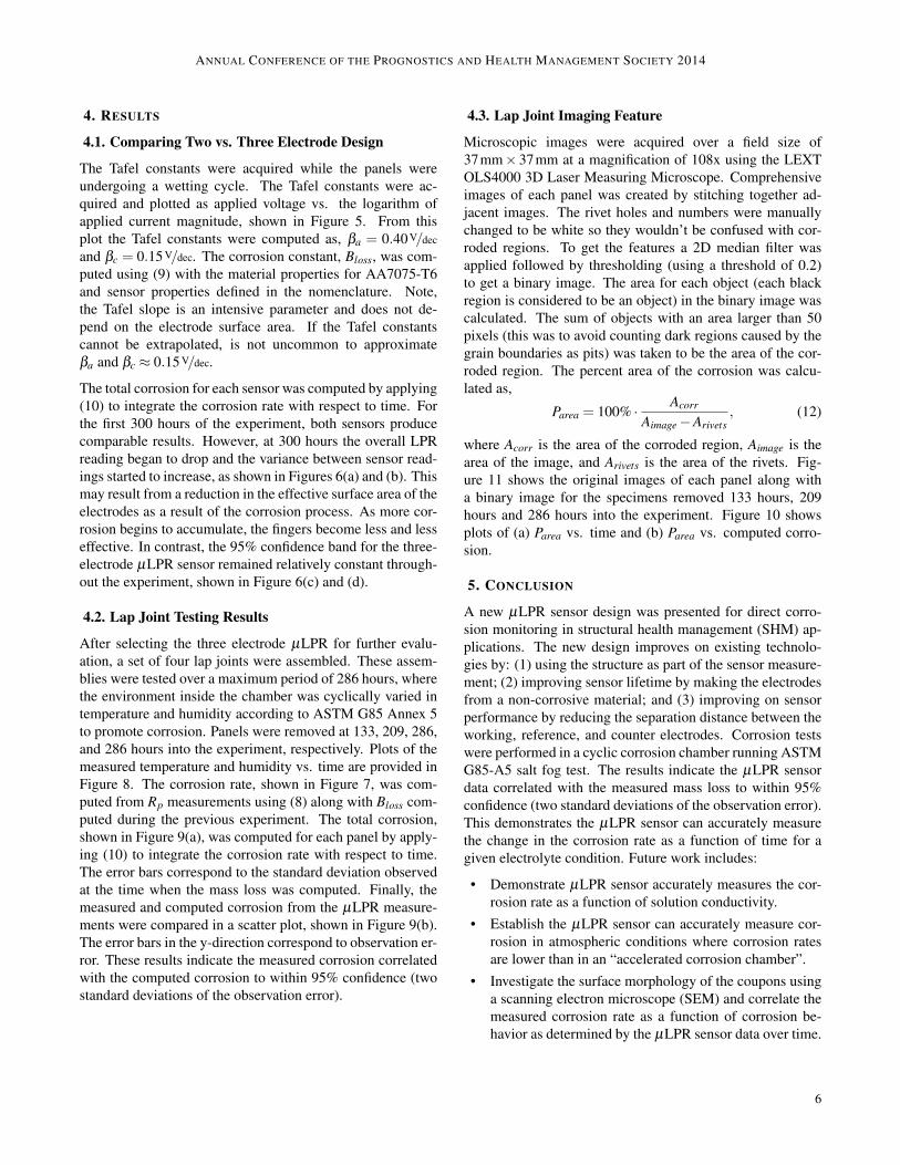
The Tafel constants were acquired while the panels wereundergoing a wetting cycle. The Tafel constants were ac-quired and plotted as applied voltage vs. the logarithm ofapplied current magnitude, shown in Figure 5. From thisplot the Tafel constants were computed as, βa = 0.40 V/dec
and βc = 0.15 V/dec. The corrosion constant, Bloss, was com-puted using (9) with the material properties for AA7075-T6and sensor properties defined in the nomenclature. Note,the Tafel slope is an intensive parameter and does not de-pend on the electrode surface area. If the Tafel constantscannot be extrapolated, is not uncommon to approximateβa and βc ≈ 0.15 V/dec.
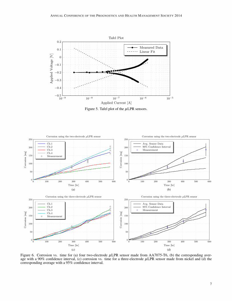
The total corrosion for each sensor was computed by applying(10) to integrate the corrosion rate with respect to time. Forthe first 300 hours of the experiment, both sensors producecomparable results. However, at 300 hours the overall LPRreading began to drop and the variance between sensor read-ings started to increase, as shown in Figures 6(a) and (b). Thismay result from a reduction in the effective surface area of theelectrodes as a result of the corrosion process. As more cor-rosion begins to accumulate, the fingers become less and lesseffective. In contrast, the 95% confidence band for the three-electrode µLPR sensor remained relatively constant through-out the experiment, shown in Figure 6(c) and (d).
4.2. Lap Joint Testing Results
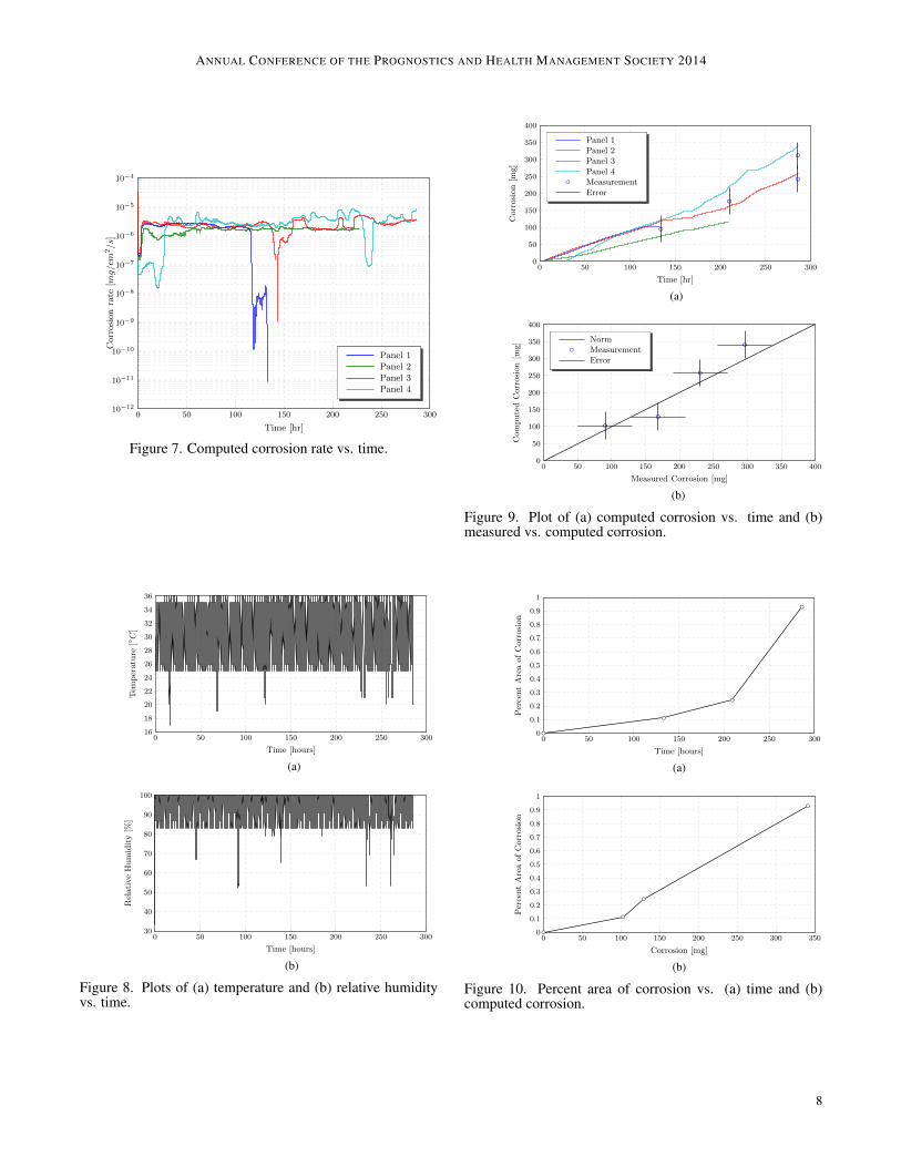
After selecting the three electrode µLPR for further evalu-ation, a set of four lap joints were assembled. These assem-blies were tested over a maximum period of 286 hours, wherethe environment inside the chamber was cyclically varied intemperature and humidity according to ASTM G85 Annex 5to promote corrosion. Panels were removed at 133, 209, 286,and 286 hours into the experiment, respectively. Plots of themeasured temperature and humidity vs. time are provided inFigure 8. The corrosion rate, shown in Figure 7, was com-puted from Rp measurements using (8) along with Bloss com-puted during the previous experiment. The total corrosion,shown in Figure 9(a), was computed for each panel by apply-ing (10) to integrate the corrosion rate with respect to time.The error bars correspond to the standard deviation observedat the time when the mass loss was computed. Finally, themeasured and computed corrosion from the µLPR measure-ments were compared in a scatter plot, shown in Figure 9(b).The error bars in the y-direction correspond to observation er-ror. These results indicate the measured corrosion correlatedwith the computed corrosion to within 95% confidence (twostandard deviations of the observation error).
4.3. Lap Joint Imaging Feature
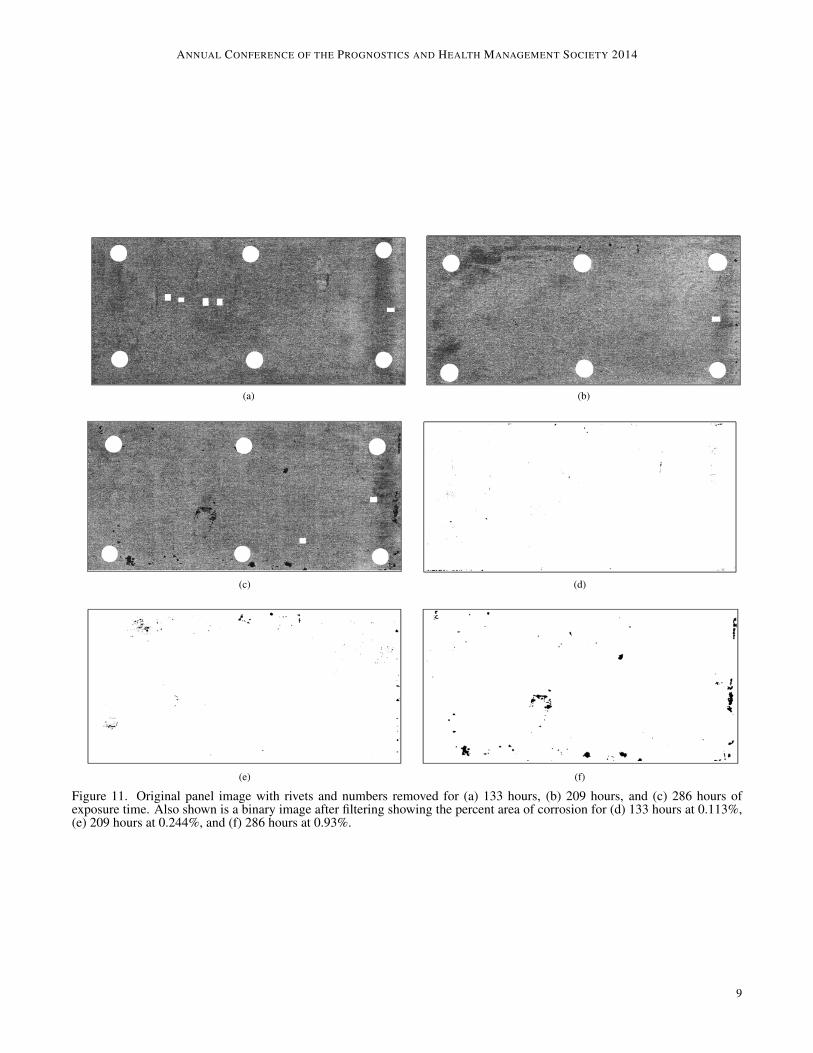
Microscopic images were acquired over a field size of37mm× 37mm at a magnification of 108x using the LEXTOLS4000 3D Laser Measuring Microscope. Comprehensiveimages of each panel was created by stitching together ad-jacent images. The rivet holes and numbers were manuallychanged to be white so they wouldn’t be confused with cor-roded regions. To get the features a 2D median filter wasapplied followed by thresholding (using a threshold of 0.2)to get a binary image. The area for each object (each blackregion is considered to be an object) in the binary image wascalculated. The sum of objects with an area larger than 50pixels (this was to avoid counting dark regions caused by thegrain boundaries as pits) was taken to be the area of the cor-roded region. The percent area of the corrosion was calcu-lated as,
Parea = 100% · Acorr
Aimage−Arivets, (12)
where Acorr is the area of the corroded region, Aimage is thearea of the image, and Arivets is the area of the rivets. Fig-ure 11 shows the original images of each panel along witha binary image for the specimens removed 133 hours, 209hours and 286 hours into the experiment. Figure 10 showsplots of (a) Parea vs. time and (b) Parea vs. computed corro-sion.
5. CONCLUSION
A new µLPR sensor design was presented for direct corro-sion monitoring in structural health management (SHM) ap-plications. The new design improves on existing technolo-gies by: (1) using the structure as part of the sensor measure-ment; (2) improving sensor lifetime by making the electrodesfrom a non-corrosive material; and (3) improving on sensorperformance by reducing the separation distance between theworking, reference, and counter electrodes. Corrosion testswere performed in a cyclic corrosion chamber running ASTMG85-A5 salt fog test. The results indicate the µLPR sensordata correlated with the measured mass loss to within 95%confidence (two standard deviations of the observation error).This demonstrates the µLPR sensor can accurately measurethe change in the corrosion rate as a function of time for agiven electrolyte condition. Future work includes:
• Demonstrate µLPR sensor accurately measures the cor-rosion rate as a function of solution conductivity.
• Establish the µLPR sensor can accurately measure cor-rosion in atmospheric conditions where corrosion ratesare lower than in an “accelerated corrosion chamber”.
• Investigate the surface morphology of the coupons usinga scanning electron microscope (SEM) and correlate themeasured corrosion rate as a function of corrosion be-havior as determined by the µLPR sensor data over time.
6
ANNUAL CONFERENCE OF THE PROGNOSTICS AND HEALTH MANAGEMENT SOCIETY 2014
10−9 10−8 10−7 10−6 10−5−0.5
−0.4
−0.3
−0.2
−0.1
0
0.1
0.2
Applied Current [A]
Applied
Voltage[V
]
Tafel Plot
bbbbbbbbbbbbbbbb
bbbbbbbbbbbbbbbb
bbbbbbbbbbbbbbbb
bbb b b b b bb b b b b b b b b bb b b b b b b b
b b b b b b b bb b b b b b b b
b b b b b b b bb b b b b b b bb b b b b b b bb b b b b
Measured DataLinear Fit
b
Figure 5. Tafel plot of the µLPR sensors.
0 100 200 300 400 500 6000
50
100
150
200
250
Time [hr]
Corrosion[m
g]
Corrosion using the two-electrode µLPR sensor
bCbCbCbCbCbCbCbC
bCbCbCbC
bCbCbCbC
bCbC
bC
bC
Ch.1Ch.2Ch.3Ch.4MeasurementbC
(a)
0 100 200 300 400 500 6000
50
100
150
200
250
Time [hr]
Corrosion[m
g]
Corrosion using the two-electrode µLPR sensor
bCbC
bCbC
bCbC
bCbC
bCbC
Avg. Sensor Data90% Confidence IntervalMeasurementbC
(b)
0 100 200 300 400 500 6000
50
100
150
200
250
Time [hr]
Corrosion[m
g]
Corrosion using the three-electrode µLPR sensor
bCbCbCbCbCbCbCbC
bCbCbCbC
bCbCbCbC
bCbC
bC
bC
Ch.1Ch.2Ch.3Ch.4MeasurementbC
(c)
0 100 200 300 400 500 6000
50
100
150
200
250
Time [hr]
Corrosion[m
g]
Corrosion using the three-electrode µLPR sensor
bCbC
bCbC
bCbC
bCbC
bCbC
Avg. Sensor Data95% Confidence IntervalMeasurementbC
(d)
Figure 6. Corrosion vs. time for (a) four two-electrode µLPR sensor made from AA7075-T6, (b) the corresponding aver-age with a 90% confidence interval, (c) corrosion vs. time for a three-electrode µLPR sensor made from nickel and (d) thecorresponding average with a 95% confidence interval.
7
ANNUAL CONFERENCE OF THE PROGNOSTICS AND HEALTH MANAGEMENT SOCIETY 2014
0 50 100 150 200 250 30010−12
10−11
10−10
10−9
10−8
10−7
10−6
10−5
10−4
Time [hr]
Corrosionrate
[mg/cm
2/s]
Panel 1Panel 2Panel 3Panel 4
Figure 7. Computed corrosion rate vs. time.
0 50 100 150 200 250 30016
18
20
22
24
26
28
30
32
34
36
Time [hours]
Tem
perature
[C]
(a)
0 50 100 150 200 250 30030
40
50
60
70
80
90
100
Time [hours]
RelativeHumidity[%
]
(b)
Figure 8. Plots of (a) temperature and (b) relative humidityvs. time.
0 50 100 150 200 250 3000
50
100
150
200
250
300
350
400
Time [hr]
Corrosion[m
g]
bCbC
bCbC
bCbC
bCbC
Panel 1Panel 2Panel 3Panel 4MeasurementError
bC
(a)
0 50 100 150 200 250 300 350 4000
50
100
150
200
250
300
350
400
Measured Corrosion [mg]
ComputedCorrosion[m
g]
bCbCbCbC
bCbC
bCbCNormMeasurementError
bC
(b)
Figure 9. Plot of (a) computed corrosion vs. time and (b)measured vs. computed corrosion.
0 50 100 150 200 250 3000
0.1
0.2
0.3
0.4
0.5
0.6
0.7
0.8
0.9
1
Time [hours]
PercentAreaofCorrosion
bC
bC
bC
bC
(a)
0 50 100 150 200 250 300 3500
0.1
0.2
0.3
0.4
0.5
0.6
0.7
0.8
0.9
1
Corrosion [mg]
PercentAreaofCorrosion
bC
bC
bC
bC
(b)
Figure 10. Percent area of corrosion vs. (a) time and (b)computed corrosion.
8
ANNUAL CONFERENCE OF THE PROGNOSTICS AND HEALTH MANAGEMENT SOCIETY 2014
(a) (b)
(c) (d)
(e) (f)
Figure 11. Original panel image with rivets and numbers removed for (a) 133 hours, (b) 209 hours, and (c) 286 hours ofexposure time. Also shown is a binary image after filtering showing the percent area of corrosion for (d) 133 hours at 0.113%,(e) 209 hours at 0.244%, and (f) 286 hours at 0.93%.
9
ANNUAL CONFERENCE OF THE PROGNOSTICS AND HEALTH MANAGEMENT SOCIETY 2014
ACKNOWLEDGMENT
All funding and development for the µLPR sensor and sys-tems in the project has been part of the US government’sSBIR programs. In particular: 1) Funding for the preparationof the initial system design and development was providedby the US Air Force under SBIR Phase II contract # F33615-01-C-5612 monitored by Dr. James Mazza; 2) Funding forthe development and experimental set-up was provided bythe US Navy under SBIR Phase II contract # N68335-06-C-0317 monitored by Dr. Paul Kulowitch; and 3) furtherimprovements, scheduled field installations, and technologytransition by the US Air Force under SBIR Phase II contract# FA8501-11-C-0012 and BAA/RIF contract # FA8650-12-C-0001 monitored by Mr. Feraidoon Zahiri.
NOMENCLATURE
βa V/dec 0.40 anodic Tafel constantβc V/dec 0.15 cathodic Tafel constantτ s - time variabledτ s - time stepk - - sample indext s - timet0 s - initial timez - 3 electron lossAcorr cm2 - % area of corrosionAimage cm2 - % area of imageArivets cm2 - % area of of rivetsAsen cm2 4.233×10⁻² sensor areaAW g/mol 2.899×101 atomic weightB? V/dec 4.95×10⁻² constantBloss Ω·g/cm2/s 1.170×10⁻⁴ constantEa V - applied potentialEcorr V - corrosion potentialIa A/cm2 - applied currentIcorr A/cm2 - corrosion currentF C/mol 9.649×10⁴ Faraday’s constantMloss g/cm2 - mass lossN - - total samplesParea - - Percent area of corrosionRloss g/cm2/s - corrosion rateRp Ω - polarization resistanceTs s 60 sample period
REFERENCES
Bockris, J. O., Reddy, A. K. N., & Gambola-Aldeco, M.(2000). Modern electrochemistry 2a. fundamentalsof electrodics (2nd ed.). New York: Kluwer Aca-demic/Plenum Publishers.
Buchheit, R. G., Hinkebein, T., Maestas, L., & Montes,L. (1998, March 22-27). Corrosion monitoring of
concrete-lined brine service pipelines using ac and dcelectrochemical methods. In Corrosion 98. San Diego,Ca.
Burstein, G. T. (2005, December). A century of tafel’s equa-tion: 1905-2005. Corrosion Science, 47(12), 2858-2870.
G102, A. S. (1994). Standard practice for calculation of cor-rosion rates and related information from electrochem-ical measurements. Annual Book of ASTM Standards,03.02.
G59, A. S. (1994). Standard practice for conducting potentio-dynamic polarization resistance measurements. AnnualBook of ASTM Standards, 03.02.
Harris, S. J., Mishon, M., & Hebbron, M. (2006, October).Corrosion sensors to reduce aircraft maintenance. InRto avt-144 workshop on enhanced aircraft platformavailability through advanced maintenance conceptsand technologies. Vilnius, Lithuania.
Herder, P., & Wijnia, Y. (2011). Asset management: Thestate of the art in europe from a life cycle perspective(T. van der Lei, Ed.). Springer.
Huston, D. (2010). Structural sensing, health mon-itoring, and performance evaluation (B. Jones &W. B. S. J. Jnr., Eds.). Taylor and Francis.
Introduction to corrosion monitoring. (2012,August 20). Online. Available fromhttp://www.alspi.com/introduction.htm
Kossowsky, R. (1989). Surface modification engineering(Vol. 1). Boca Raton, Florida: CRC Press, Inc.
Twomey, M. (1997). Inspection techniques for detecting cor-rosion under insulation. Material Evaluation, 55(2),129-133.
Wagner, C., & Traud, W. (1938).Elektrochem, 44, 391.
BIOGRAPHIES
Douglas W. Brown is the Senior Systems Engineer forAnalatom, Inc. He received the bachelor of science degree inelectrical engineering from the Rochester Institute of Tech-nology and his master of science and doctor of philosophydegrees in electrical engineering from the Georgia Instituteof Technology. Dr. Brown has ten years of experience de-veloping and maturing Prognostics & Health Management(PHM) and fault-tolerant control systems in avionics appli-cation. He is a recipient of the National Defense Scienceand Engineering Graduate (NDSEG) Fellowship and has re-ceived several best-paper awards for his work in PHM andfault-tolerant control.
Richard J. Connolly is the Senior Research Engineer forAnalatom, Inc. He completed his bachelor of science anddoctor of philosophy degree in chemical and biomedical en-gineering at the University of South Florida. Dr. Connolly is
10
ANNUAL CONFERENCE OF THE PROGNOSTICS AND HEALTH MANAGEMENT SOCIETY 2014
a fellow of the National Science Foundation and is regardedas an expert in interfacing of engineering devices with skin.He has extensive experience in bioelectrics, electrochemistry,and data analysis. Much of this experience was gained whileperforming bioelectric data collection on human and animalmodels. During his tenure at Analatom he has overseen test-ing and validation of the µLPR technology for aerospace andcivil engineering applications.
Bernard Laskowski is the President and Senior ResearchScientist at Analatom since 1981. He received the licen-tiaat and doctor of philosophy degrees in physics from theUniversity of Brussels in 1969 and 1974, respectively. Dr.Laskowski has published over 30 papers in internationalrefereed journals in the fields of micro-physics and micro-chemistry. As president of Analatom, Dr. Laskowski hasmanaged 93 university, government, and private industry con-tracts, receiving a U.S. Small Business Administration Ad-ministrator’s Award for Excellence.
Margaret Garvan received her master of science degree inelectrical and computer engineering (ECE) from the GeorgiaInstitute of Technology, and bachelor of science in electricalengineering from the University of Florida. She is currently aPh.D. candidate and graduate research assistant at the Geor-gia Institute of Technology. Her research is focused on intel-ligent machine learning, and methodologies for diagnosticsand prognostics for structural health monitoring.
Honglei Li received her master of science degree in electricaland computer engineering (ECE) from the Georgia Instituteof Technology, and in Instrumental Engineering from Shang-hai Jiao Tong University respectively. She is currently a grad-uate research assistant at Intelligent Control Systems Labora-tory, working on her doctoral degree in ECE at the GeorgiaInstitute of Technology. Her current research is focused onintelligent machine learning, methodologies for prognosticsand structural health monitoring and health management, aswell as asset life-cycle and risk management.
Vinod S. Agarwala Dr. Vinod S. Agarwala is a recently re-tired from the U.S. Civil Service as a Navy senior staff sci-entist and Esteemed Fellow of Naval Air Systems Command,Patuxent River, MD. He received a bachelor of science de-gree in Physics, Chemistry and Mathematics, two masters ofscience degrees, and a doctor of philosophy degree in Chem-istry and Metallurgy from Banaras Hindu University (India)and Massachusetts Institute of Technology (USA). He has 35years of distinguished civil service with major contributionsin aircraft research and development technologies; he wasawarded Department of The Navy Superior Civilian ServiceMedal. From 2006 - 2008, he was Associate Director at theU. S. Office of Naval Research Global - London, UK. Therehe served as an international agent for U.S. Navy with a mis-sion to encourage international collaboration in Science andTechnology through priority R&D in support of U.S. Navalforces.
George Vachtsevanos is a Professor Emeritus of Electricaland Computer Engineering at the Georgia Institute of Tech-nology. He was awarded a B.E.E. degree from the City Col-lege of New York in 1962, a M.E.E. degree from New YorkUniversity in 1963 and the Ph.D. degree in Electrical En-gineering from the City University of New York in 1970.He directs the Intelligent Control Systems laboratory at theGeorgia Institute of Technology where faculty and studentsare conducting research in intelligent control, neurotechnol-ogy and cardiotechnology, fault diagnosis and prognosis oflarge-scale dynamical systems and control technologies forUnmanned Aerial Vehicles. His work is funded by govern-ment agencies and industry. He has published over 240 tech-nical papers and is a senior member of IEEE. Dr. Vachtse-vanos was awarded the IEEE Control Systems Magazine Out-standing Paper Award for the years 2002-2003 (with L. Willsand B. Heck). He was also awarded the 2002-2003 GeorgiaTech School of Electrical and Computer Engineering Distin-guished Professor Award and the 2003-2004 Georgia Insti-tute of Technology Outstanding Interdisciplinary ActivitiesAward.
11