A new instrument for measuring the high dynamic range ...rads.physics.miami.edu/optics/ken/RefPapers/079_WDLMV_OE_2012.pdf · A new instrument for measuring the high dynamic range

A new instrument for measuring the high dynamic range radiance distribution in near-

surface sea water

Jianwei Wei,1 Ronnie Van Dommelen,2 Marlon R. Lewis,1,2,* Scott McLean,3 and Kenneth J. Voss4

1Department of Oceanography, Dalhousie University, Halifax, Nova Scotia, B3H 4J1, Canada 2Satlantic LP, Halifax, Nova Scotia, B3K 5X8, Canada

3Ocean Networks Canada, Victoria, British Columbia, V8W 2Y2, Canada 4Department of Physics, University of Miami, Coral Gables, Florida, 33124, USA

*[email protected]

Abstract: A new instrument for measuring the full radiance distribution in the ocean interior is introduced. The system is based on CMOS technology to achieve intra-scene dynamic range of 6 decades and system dynamic range of more than 9 decades. The spatial resolution is nominally 0.5 degrees with a temporal frame rate between 1 and 15 frames per second. The general instrumentation, detailed calibration, and a characterization of the system are described. Validity of the camera systems is demonstrated by comparison of the radiance measurements with other classical oceanographic radiometers.

©2012 Optical Society of America

OCIS codes: (010.4450) Oceanic optics; (280.0280) Remote sensing and sensors; (120.5630) Radiometry; (350.4600) Optical engineering; (010.1290) Atmospheric optics.

References and links

1. N. G. Jerlov, Marine Optics (Elsevier Scientific Publishing Company, Amsterdam, 1976), p. 231. 2. N. G. Johnson and G. Liljequist, “On the angular distributions of submarine daylight and on the total submarine

illumination,” Sven. Hydrogr. - Biol. Komm. Skr., Ny Ser. Hydrogr. 14, 1–15 (1938). 3. H. Pettersson, “Measurements of the angular distribution of submarine light,” Rapp. Cons. Explor. Mer. 108, 7–

12 (1938). 4. L. V. Whitney, “The angular distribution of characteristic diffuse light in natural waters,” J. Mar. Res. 4, 122–

131 (1941). 5. J. E. Tyler, “Radiance distribution as a function of depth in the submarine environment,” SIO Ref. 58–25(1958). 6. T. Sasaki, S. Watanabe, G. Oshiba, and N. Okami, “Measurements of angular distribution of submarine daylight

by means of a new instrument,” J. Oceanogr. Soc. Jpn 14, 47–52 (1958). 7. N. G. Jerlov and M. Fukuda, “Radiance distribution in the upper layers of the sea,” Tellus 12(3), 348–355

(1960). 8. B. Lundgren and N. K. Højerslev, “Daylight measurements in the Sargasso sea. Results from the ‘Dana’

expedition (January-April 1966),” 14 (Department of Physical Oceanography, University of Copenhagen, Copenhagen, 1971).

9. K. J. Voss and G. Zibordi, “Radiometric and geometric calibration of a visible spectral electro-optic fisheye camera radiance distribution system,” J. Atmos. Ocean. Technol. 6(4), 652–662 (1989).

10. K. J. Voss, A. Morel, and D. Antoine, “Detailed validation of the birectional effect in various case 1 waters for application to ocean color imagery,” Biogeosciences 4(5), 781–789 (2007).

11. A. A. Gershun, “The light field (translated in English by P. Moon and G. Timoshenko),” J. Math. Phys. 18, 51–151 (1939).

12. S. Q. Duntley, R. J. Uhl, R. W. Austin, A. R. Boileau, and J. E. Tyler, “An underwater photometer,” J. Opt. Soc. Am. 45, 904A (1955).

13. E. Aas and N. K. Højerslev, “Analysis of underwater radiance observations: apparent optical properties and analytic functions describing the angular radiance distribution,” J. Geophys. Res. 104(C4), 8015–8024 (1999).

14. R. C. Smith, R. W. Austin, and J. E. Tyler, “An oceanographic radiance distribution camera system,” Appl. Opt. 9(9), 2015–2022 (1970).

15. R. C. Smith, “Structure of solar radiation in the upper layers of the sea,” in Optical Aspects of Oceanography N.G. Jerlov and E.S. Nielsen, eds. (Academic Press, London and New York, 1974), pp. 95–119.

#175679 - $15.00 USD Received 6 Sep 2012; revised 29 Oct 2012; accepted 6 Nov 2012; published 15 Nov 2012(C) 2012 OSA 19 November 2012 / Vol. 20, No. 24 / OPTICS EXPRESS 27024

16. K. J. Voss and A. Chapin, “Upwelling radiance distribution camera system, NURADS,” Opt. Express 13(11), 4250–4262 (2005).

17. K. J. Voss, C. D. Mobley, L. K. Sundman, J. E. Ivey, and C. H. Mazel, “The spectral upwelling radiance distribution in optically shallow waters,” Limnol. Oceanogr. 48(1_part_2), 364–373 (2003).

18. M. R. Lewis, J. Wei, R. van Dommelen, and K. J. Voss, “Quantitative estimation of the underwater radiance distribution,” J. Geophys. Res. 116, C00H06 (2011), doi:10.1029/2011JC007275.

19. M. Darecki, D. Stramski, and M. Sokolski, “Measurements of high-frequency light fluctuations induced by sea surface waves with an underwater porcupine radiometer system,” J. Geophys. Res. 116, C00H09 (2011), doi:10.1029/2011JC007338.

20. K. Miyamoto, “Fish eye lens,” J. Opt. Soc. Am. 54(8), 1060–1061 (1964). 21. K. J. Waters, R. C. Smith, and M. R. Lewis, “Avoiding ship-induced light-field perturbation in the determination

of oceanic optical properties,” Oceanography (Wash. D.C.) 3, 18–21 (1990). 22. F. E. Nicodemus, Self-study Manual on Optical Radiation Measurements: Part I - Concepts, Chapters 4 and 5

(U.S. Government Printing Office, Washington, 1978), p. 118. 23. H. Du and K. J. Voss, “Effects of point-spread function on calibration and radiometric accuracy of CCD

camera,” Appl. Opt. 43(3), 665–670 (2004). 24. G. Zibordi, S. B. Hooker, J. Mueller, and G. Lazin, “Characterization of the immersion factor for a series of in-

water optical radiometers,” J. Atmos. Ocean. Technol. 21(3), 501–514 (2004). 25. T. H. Waterman, “Polarization patterns in submarine illumination,” Science 120(3127), 927–932 (1954). 26. C. L. Wyatt, V. Privalsky, and R. Datla, Recommended Practice: Symbols, Terms, Units and Uncertainty

Analysis for Radiometric Sensor Calibration (U.S. Dept. of Commerce, Washington, D.C., 1998), p. 120. 27. K. J. Voss, S. McLean, M. R. Lewis, C. Johnson, S. Flora, M. Feinholz, M. Yarbrough, C. C. Trees, M. S.

Twardowski, and D. K. Clark, “An example crossover experiment for testing new vicarious calibration techniques for satellite ocean color radiometry,” J. Atmos. Ocean. Technol. 27(10), 1747–1759 (2010).

28. A. W. Harrison and C. A. Coombes, “An opaque cloud cover model of sky short wavelength radiance,” Sol. Energy 41(4), 387–392 (1988).

29. M. Stramska and T. D. Dickey, “Short-term variability of the underwater light field in the oligotrophic ocean in response to surface waves and clouds,” Deep Sea Res. Part I Oceanogr. Res. Pap. 45(9), 1393–1410 (1998).

1. Introduction

Radiance is the total radiant energy of photons per unit solid angle per unit surface area and per unit time [1]. The angular distribution of radiance in the upper water column is of fundamental importance for many problems met in aquatic sciences and accurately measuring the underwater radiance distribution has been one of the critical tasks in hydrologic optics [2–10].

One of the earliest instruments for in-water radiance was a screened photometer designed by Johnson and Liljequist [2] and Pettersson [3]. This apparatus consisted of an irradiance meter (with a horizontal receiving surface) and a movable black plate. The plate was suspended above the irradiance sensor, and moved along the vertical to yield a sum of azimuthally averaged radiances over different zenith intervals. This instrument was later modified to measure the radiance over azimuthal directions replacing the overhead screen with a cylindrical screen so that the photometer received light from a narrow cone (half angle α1/2 = 7.5°). The primitive instruments provided the earliest picture of the depth evolution of the radiance field underwater [also see 4].

A convenient design for a radiance sensor is the Gershun-tube [11] radiometer. One early development in this approach was the Scripps radiance photometer [12]. For in-water operation, the radiometer was suspended by a cable and rotated so that it measured the radiance in different directions [5–8]. Spatial scanning with coarse resolutions around 10-30° along both the zenith and azimuthal directions required about 10-20 minutes at only one depth [e.g 5.], limiting the conditions under which it could be deployed. As well, the large field of view (FOV), α1/2 = 3.5°-7.5°, results in averaging out many fine features pertinent to the radiance field. A similar instrument has also been deployed by Aas and Højerslev [13].

The first development of a radiance camera system to instantaneously image the radiance distribution underwater was completed by Smith, Austin and Tyler [14]. Their instrument relied on a fisheye lens and a film camera. The fisheye lens projected the incoming hemispheric light onto the image plane (see Fig. 1), and the radiance was related to the density of the exposed film negative [15]. A more advanced radiance camera was built by


Voss and Chapin [16], based on solid state cameras (e.g. CCD). The CCD radiance camera measures the full radiance distribution with very low noise and very high spatial resolution (~0.5°); it has provided the most complete data for the upwelling radiance distribution in various waters [10, 16, 17]. However, as the CCD radiance cameras are based on linear system transfer functions, they are prone to saturation when viewing scenes including extremely intense radiation like direct sunlight in the near-surface water.

The radiance distribution in the sea is a consequence of the refraction of the radiance distribution from the sun and sky at the air-sea interface and the subsequent light absorption and scattering within the water itself. These phenomena result in an anisotropic in-water radiance field. For example, the downwelling radiance distribution varies over a dynamic range of more than 6 decades [5, 18], while the intra-scene dynamic range for the upwelling light rarely exceed two decades [16, 18]. Furthermore, in open ocean areas, the sea surface is rarely a static environment and this results in fluctuations of less than one second in the underwater light field [19]. An ideal instrument to measure the in-water radiance distribution requires a radiometer that is calibrated against international standards over a wide dynamic range, and that can take synoptic observations with a fine angular resolution.

The objective of this study is to describe a new high dynamic range (HDR) solid-state camera system (RadCam), capable of measuring the full radiance field at high temporal and angular frequency in the upper ocean. The basic configuration of the camera system is introduced in Section 2. We describe steps taken to calibrate and characterize the sensor in Section 3. The measurement uncertainty is estimated in Section 4. A few example measurements of the radiance distribution in natural environments are demonstrated in Section 5, followed by a discussion and summary in Section 6.

Zenith

φ

θx

y

(x′,y′)

Image plane

Fisheye lens∆A1

∆A2

O1

O2 x΄

y΄

Fig. 1. Schematic drawing of the geometry for measuring directional radiance. Camera with fisheye lens maps the radiance L(θ,φ) in one hemispheric space onto the image plane, which is defined by pixel (x',y').

2. RadCam instrument

The design of the RadCam radiometer is inspired by previous underwater fisheye radiance cameras [9, 14, 16], with the above-mentioned challenges in mind. A high dynamic range sensor was used as the imaging element.

2.1 Fisheye lens and input optics

The optical components of the radiance camera are composed of a fisheye lens (Coastal Optics Systems) and a customized optical relay system. The layout of the optical system is shown in Fig. 2. The fisheye lens covers a hemispherical field of view and follows an


equidistant projection (radius on image is linearly proportional to field angle θ). The assembled underwater camera employs a BK-7 glass dome (not shown in the figure) to protect the lens. The relay uses a pair of achromatic doublet lenses to achieve the desired image magnification. A triplet field lens is also employed to increase the FOV of the relay and to reduce the lens system roll-off. A spectral bandpass filter is inserted into the relay system, so that the optical system projects light centered at 555 nm, with 20 nm bandwidth on the detector array. The optical system projects a circular image of a hemisphere of the radiance distribution. All optical components except the dome and array are antireflection coated.

Fig. 2. Camera components and configuration. (a) Schematic of the optical system including the fisheye lens and optical relay. (b) Picture of the assembled optical system with the CMOS camera. (c) Picture of the customized camera- head electronics. The silver rectangular box in (c) is the fiber transceiver.

2.2 CMOS imager

The imager used in our camera is a Micron® Complementary Metal Oxide Semiconductor (CMOS) image sensor. The CMOS technology allows the incorporation of on-chip electronics with the photo-detectors. The on-chip electronics allows increased functionality, for example, to obtain the high intra-scene dynamic range using a variety of response functions. The CMOS array is also inherently non-blooming and capable of measuring radiant flux up to 9 orders of magnitude, which is critical for imaging the full radiance field including the sun. Some shortcomings are also apparent, however, like increased noise and reduced uniformity; some of which can be minimized and accounted for by a complete radiometric calibration. The CMOS array has 752 × 480 pixels, each 6 × 6 μm in size. It employs a global shutter that prevents smearing of the dynamic scenes. A frame grabber is used to digitize the video signal into a 2D rectangular array of 10-bit integer values.

The circular image captured by the array is represented by a total of πD2/4 pixels, where D is the diameter of the captured image described in number of pixels. Since the fisheye lens follows the equidistant projection, the pixel position in the image plane is proportional to the direction of the incident ray [20]

r α θ= ⋅ (1)

where r is the radial distance of the active pixel from the image center (also in number of pixels), α is a constant, and θ is the field angle of incoming ray relative to the principal optical


axis. These geometrical parameters are determined empirically during the initial characterization.

The electronics on the chip surrounding the array are sensitive to the incident light and produces a spatially nonuniform pixel gain. The chip incorporates a shield to reduce this effect, but during calibration we needed to illuminate the whole array with high intensity light and this shield is not sufficient. We overcame this problem by attaching a black metal shield directly on top of the chip. This reduces the effective array size to less than 420 pixels in diameter.

The system's acquisition speed is greater than 40 frames per second (fps) for the shortest exposure time that we use. However, the recorded frame rate is limited by the logging computer system (particularly the custom software) to 15 frames per second (fps). At the lowest light levels, for example when measuring the radiance distribution at depth under a cloudy sky, the system is limited to about 1 fps due to an extended exposure time.

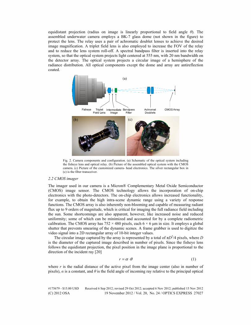
2.3 Camera system

Three types of radiance distribution camera systems have been built with the same configuration of the optical systems and imagers: a water-column profiling camera, a sky camera, and a self-logging camera. All three camera systems are assembled in aluminum housings. They all include a tilt/compass sensor (Advanced Orientation System) to record the pitch, roll and yaw of the instrument.

The profiler in Fig. 3(a) is equipped with dual cameras, one looking upward and the other one viewing downward. The two cameras together image the full radiance field. This system is designed for free-fall operation [21] with two fins installed on the upper end of the housing, symmetric about the camera. A CTD sensor (Falmouth Scientific) and multichannel OCR-504I/R radiometers (Satlantic LP) are set up on each fin with the upward viewing instrument measuring the planar irradiance and the downward looking instrument measuring the nadir radiance. Both are operated at four wavelengths (412, 443, 490 and 555 nm). The instrument buoyancy is adjusted by adding/removing foam from inside the fins so that the package descends at a speed of less than 0.5 m s−1. With this arrangement, the instrument's tilt is generally less than 5° except in the first few meters below the sea surface. The fins also help the instrument package trail away from the deployment vessel before data collection. A guard cage is used to protect the upwelling camera window. The overall height for the profiler is 115 cm, the width is 46 cm (distance including the two fins), and the weight in air is 26 kg. The depth rating is 200 m. The profiling system communicates with the on-deck computer running logging software via a fiber optic cable. The ancillary data including the downwelling irradiance and upwelling nadir radiance from the OCR-504I/R sensor, CTD data and tilt and heading information are synchronized with the image data and saved in a separate file.

The sky camera in Fig. 3(b) images the full sky radiance distribution including the sun without the glass dome. It communicates with the same control computer via a separate fiber optic cable. This camera system is 36 cm in height and 11 cm in diameter, and weights 3.8 kg in air. This camera is designed to work simultaneously with the profiling camera, to provide information on the incident light above the sea surface, but can also operate independently.

The third camera system is a self-logging camera specifically designed for operations on various underwater platforms such as an autonomous underwater vehicle (AUV). An on-board custom computer controls the camera and internally logs the radiance data where it is downloaded when the system is recovered. This system is 26 cm in height and 23 cm in diameter and the weight in air is about 9.6 kg. The logging camera can also be mounted in a cage as shown in Fig. 3(c) and lowered into the water from a boom to make depth profiles in one hemisphere.


Fig. 3. Radiance distribution camera systems. (a) Profiling camera. The downwelling camera is on the top and the upwelling camera is at the bottom; OCR-504I/R radiometers are installed on the left wing and the CTD is on the right wing. (b) Sky camera mounted on a tripod. (c) Self-logging underwater radiance camera mounted in a cage. Image courtesy of Satlantic LP.

3. Radiometric and geometric calibration and characterization

The general form of the calibration equation describes the spectral radiance L(λ) as a function of the output signal [22]

[ ]( ) ( )L f sλ λ= (2)

where s is the output signal per unit of input, in this case, the radiance. The wavelength dependency will be dropped since only one wavelength is considered in our cameras. The absolute radiance responsivity function f is an essential parameter to be determined in calibrations.

A complete calibration of the sensor requires corrections in several domains be applied to the measurement equation. The system is designed to be nonlinear over the dynamic range of response. Characterizing the nonuniformity of pixel-to-pixel response for the array detector is also critical in the spatial (angular) domain. The modulation transfer function (MTF) of the optical system is another parameter to be determined to make necessary corrections in the system level calibration.

3.1 HDR response functions

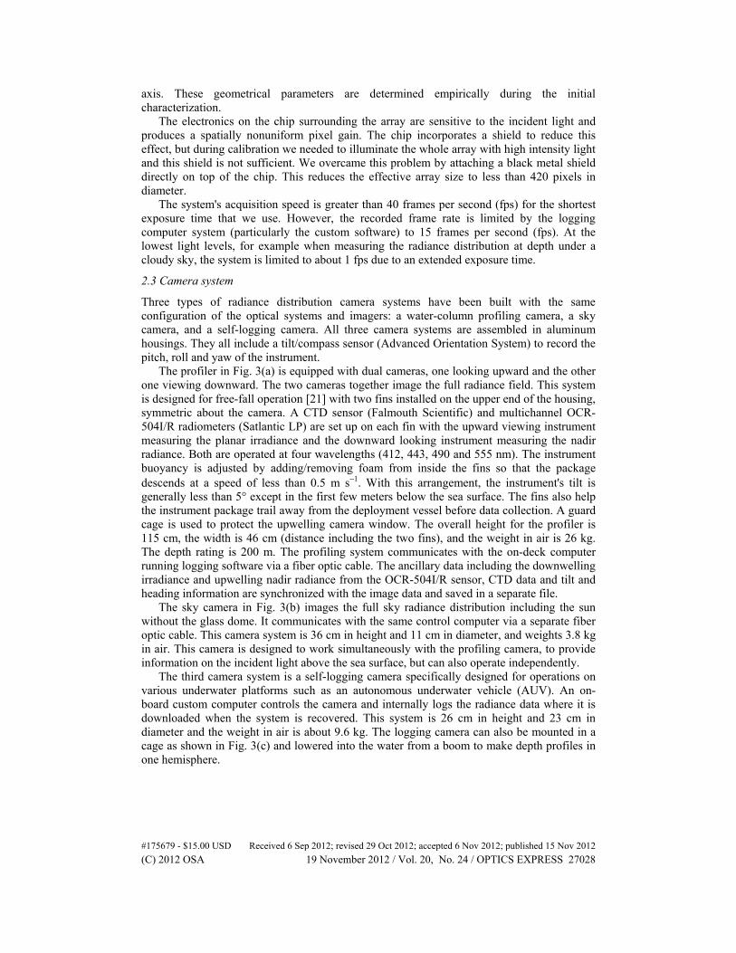
The first step in the calibration is to define the shape of high dynamic range response functions over the 210 gray scales in the range of camera counts from 0 to 1023. Different combinations of register settings including the shutter widths, vertical blanking and potential barrier limits, etc., were tested with the bare imager (no optical system) illuminated by a 1000 w FEL lamp (Fig. 4(a)). The incoming light flux was varied by adding neutral density (ND) filters between the imager and the lamp. The incident radiation was also changed by moving the imager relative to the light source. For higher incident radiance, a Helium-Neon laser beam was used to illuminate pixels on the array (Fig. 4(b)). Three sets of register settings were determined after the experimentation, which are regarded as the low, mid and high exposure settings in our study. For each exposure setting, the pixel responds to the incident light in a characteristic way. Figure 5(a) presents three example response curves representative of distinctive exposure settings, where the output signals s are described as a


function of the irradiance. The three response curves cover relatively low, moderate, and high radiance ranges and partly overlap. The moderate and high exposures each permit intra-scene contrasts of more than 6 decades (60 dB) and the total range is over 9 decades (90 dB). Exposure time ranges between 0.02 and 1.0 seconds. Each curve can be divided into several segments and each segment is fit to a simple model; the goodness of fit is usually better than 0.99. The high-exposure response curve is designed to measure the most intense light, such as the radiance distribution in near-surface sea water, and the exposure time is approximately 0.02 seconds in this case.

The pixels on the CMOS array have their own amplifiers. Each active pixel behaves as an independent radiance sensor, receiving photons, converting them to a voltage and transferring the information directly to the output. To account for the potential nonuniformity of the pixel array, a flat-field correction was performed. This calibration first measures the response of each pixel to the same light source (FEL lamp) (Fig. 4(a)). The second step involves the use of a Helium-Neon laser as the light source, with the CMOS imager being mounted on a precision three-axis translation stage (Fig. 4(b)). The array was scanned across the laser beam, to build up a composite calibration image. Neutral density filters were also used in this step to vary the incident light flux. We note that the intensity profile of the laser beam is actually a Gaussian shape. A single pixel on the array was therefore used to scan across the laser beam and determine the beam radius (in pixels) that is suitably uniform to be used for calibration.

526x

y

O

11’ 2 3 4

(a)

(b)

3

(c)

9

8 2

10

73

3

1

Fig. 4. Experimental setup.(a) The pixel array receives the light emitting from the 1000 w FEL lamp. (b) The pixel array is scanned with the laser beam. (c) The assembled camera receives light from the integrating sphere. The experimental components consist of 1) the bare imager, 2) neutral density filter, 3) light baffle, 4) FEL lamp, 5) Helium-Neon laser, 6) XYZ translator, 7) integrating sphere, 8) arc lamp, 9) assembled camera and 10) rotation stage; 1') shows the same bare imager mounted at a distance different from that indicated by 1).

3.2 Absolute responsivity

The purpose of the system calibration is to convert the response curve to absolute responsivity for every pixel. For this calibration, the imager and the optics were assembled together. For the underwater camera, the glass dome was installed as well. Figure 4(c) shows the experimental setup for the system calibration. The integrating sphere was set up on the optical bench and illuminated by an arc lamp. The camera was mounted onto a rotation stage with its lens toward the sphere's exit and imaged the light exiting the sphere. The camera's lens was scanned over the full 180° as the camera was rotated. The end result is a bright circular image covering the entire hemispheric field of view. The absolute radiance of the light exiting the sphere was measured with a transfer radiometer (HyperOCR, Satlantic LP), which was calibrated with a NIST-traceable radiometric calibration transfer standard. This image of absolute radiance is then used to scale the relative response curves to an absolute responsivity.

This experimental setup is necessary to achieve the high radiance values required. The typical method for radiance calibration using an FEL lamp and a planar Lambertian plaque [e.g 9.] does not provide a source with sufficient energy. The roll-off of the optical system is


less than 8% at θ = 90° due to the use of a field lens at the output of the fisheye lens. The system level calibration performed by rotating the camera has calibrated every pixel and in theory has removed the system's roll-off. The beam spreading effect requires the point spread function (PSF) and is described below. This system level calibration is carried out for the other two exposure settings by inserting neutral density filters between the integrating sphere and the arc lamp.

3.3 Geometric projection

The camera was mounted onto the rotation stage as in previous experiments. A green light-emitting diode (LED) was positioned at the same height and at a distance of at least 1 m from the camera lens. This arrangement allows the LED emitted light to be completely imaged by a single pixel. The scanning was done at 1° steps throughout the hemispheric field of view of the camera and then with the camera head rolled about its principal axis. Two such scanning lines can be used to define the location for the image center and the diameter D with simple trigonometry.

As implied in Eq. (1), the radial distance r of the active pixel from the image center (x, y) conforms to the linearity, r = Dθ/π, where θ is the polar direction of the incident ray sensed by the active pixel. This test indicates that the geometrical projection is linear (Fig. 5(b)), with an r2 = 0.999. For a system with an image diameter D = 400 pixels, the measured radiance field has the nominal spatial resolution of ~0.45° along the radial direction (i.e. the zenith direction in the spherical coordinate). The azimuthal resolution is related to the pixel's radial distance. For example, the resolution is about ∆φ = 10° at polar angle 5° and increases to ∆φ = 1° at polar position 45°. The solid angle dΩ(i,j) subtended by a pixel area (dA) also varies with its radial distance in the image plane [also see 16] and can be represented as

( , ) sin( )ij

ij

ld i j dA

l D D

ππΩ = ⋅ ⋅ (3)

According to Eq. (3), the solid angle dΩ(i,j) for each active pixel is slightly dependent on the radial distance. For example, the dΩ is about 6.46 × 10−5 sr near the Zenith and decreases to 4.77 × 10−5 sr at zenith angle θ = 85°.

3.4 Point spread function

Beam spreading will also affect the accuracy of the radiometric measurement [e.g [23].]. The point spread function (PSF) of the optical system was measured to account for this effect, which is also known as the beam spread function (BSF). A beam expander was used to expand the Helium-Neon laser beam so that the entire camera's dome was illuminated by the incoming light. The imager array was set to operate in linear mode and multiple exposures used to achieve the complete dynamic range needed to measure the PSF out to the largest radii. The point spread function is assumed to be spatially-invariant and is derived by binning and averaging the camera response (in digital counts) as a function of the radial distance from the image center (x, y). The PSF varies up to 6 orders of magnitude in digital counts, from the center of a point source to the 200th pixel (Fig. 5(c)). The measured point spread function was applied by an iterative image deblurring approach using the Lucy-Richardson algorithm. This method was chosen because the radiant energy can be conserved during the calculation, which is critical for the absolute radiometric output.

3.5 Immersion factor

When immersed in the sea water, the ambient light enters the camera through the water-glass-air path. The index of refraction of sea water (nw = 1.34) will impact the absolute responsivity determined in air [e.g [24].]; an immersion factor that accounts for the change in absolute responsivity must be determined. The experimental procedure of Voss and Chapin [16] was


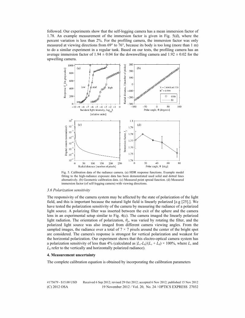
followed. Our experiments show that the self-logging camera has a mean immersion factor of 1.78. An example measurement of the immersion factor is given in Fig. 5(d), where the percent variation is less than 2%. For the profiling camera, the immersion factor was only measured at viewing directions from 69° to 76°, because its body is too long (more than 1 m) to do a similar experiment in a regular tank. Based on our tests, the profiling camera has an average immersion factor of 1.94 ± 0.04 for the downwelling camera and 1.92 ± 0.02 for the upwelling camera.

Fig. 5. Calibration data of the radiance camera. (a) HDR response functions. Example model fitting to the high-radiance exposure data has been demonstrated used solid and dotted lines alternatively. (b) Geometric calibration data. (c) Measured point spread function. (d) Measured immersion factor (of self-logging camera) with viewing directions.

3.6 Polarization sensitivity

The responsivity of the camera system may be affected by the state of polarization of the light field, and this is important because the natural light field is linearly polarized [e.g [25].]. We have tested the polarization sensitivity of the camera by measuring the radiance of a polarized light source. A polarizing filter was inserted between the exit of the sphere and the camera lens in an experimental setup similar to Fig. 4(c). The camera imaged the linearly polarized light radiation. The orientation of polarization, θp, was varied by rotating the filter, and the polarized light source was also imaged from different camera viewing angles. From the sampled images, the radiance over a total of 7 × 7 pixels around the center of the bright spot are considered. The camera's response is strongest for vertical polarization and weakest for the horizontal polarization. Our experiment shows that this electro-optical camera system has a polarization sensitivity of less than 4% (calculated as |Lv-Lh|/(Lv + Lh) × 100%, where Lv and Lh refer to the vertically and horizontally polarized radiance).

4. Measurement uncertainty

The complete calibration equation is obtained by incorporating the calibration parameters


1[ ] PSFfL f s I ρ −= ⋅ ⋅ ⋅ (4)

where the absolute responsivity f is fitted to polynomial functions of the sensor response s, f[s] = p1s

n + p2sn−1 + … + pn+1, with polynomial coefficients pn; If is the immersion factor; ρ is

the spectral response function (SRF); and PSF is a mathematic operator rather than a scalar, representing the introduction of the PSF correction. Uncertainties of the calibration parameters propagate to the radiance measurements.

Uncertainty of f[s] is subject to the quantization noise and errors of the raw sensor response. The temporal variation of the absolute measurement was estimated by continuously imaging the integrating sphere illuminated by the arc lamp as shown in Fig. 4(c). The relative uncertainty is calculated as the ratio of the standard deviation of the mean to the mean of the radiance measurements, which has been shown generally to be less than 2% (Table 1). The estimate for temporal uncertainty includes contributions from variations in the light source.

Table 1. Uncertainty of the sensor responsivity as determined from the radiance measurements (555 nm).

Hi-exposure measurements Mid-exposure measurements

Mean radiance* 211 89 51 6.9 5.9 3.47 1.70 0.73 0.31 0.07 0.03

Relative uncertainty (%)

0.05 0.06 0.24 0.56 0.84 1.10 0.85 1.09 0.07 0.45 0.48

| | | | | | | | | | |

3.11 1.13 0.50 1.11 1.20 1.30 1.56 1.59 0.30 0.98 1.05

*unit: μWcm−2sr−1nm−1

The description of the response function f[s] may be incomplete since that the available experimental data for establishing the nonlinear fitting models are limited by the experimental setups. This uncertainty due to insufficient formulation remains unknown, however. One consequence is that the model fittings applied to every pixel will generate residual variations in the flat field, causing the reproducibility variation. We have tested the residual spatial uniformity of radiance measurements over the field of view of the camera in a setup similar to Fig. 4(c). The camera was rotated horizontally in steps of approximately 10° from 2° to 86°, while the output light from the integrating sphere was imaged. Groups of 7 × 7 pixels were averaged for each field angle. The results are listed in Table 2, which shows a measurement uncertainty generally less than 10%. This pixel-to-pixel variation is mainly contributed by the variation of the absolute responsivity in the spatial domain.

Table 2. Large scale uniformity determined as the relative uncertainty of radiance measurements (555 nm) in ten different field angles from 2° to 86°.

Radiance measurements

Mean radiance* 300 180 50 6.5 9.5 8.6 4.4 2.2 1.1 0.30 0.07 0.04

Exposure setting hi hi hi hi mid mid mid mid mid mid mid mid

Relative uncertainty (%)

9.7 10.2 0.8 1.4 3.3 4.1 6.0 3.2 2.1 2.9 13.7 5.2

*unit: μWcm−2sr−1nm−1

The SRF has a FWHM of λFWHM = 19.8 nm with a standard deviation 0.06 nm. To estimate the uncertainty, we assumed a single line-source falling within nominal band of 546 nm to 564nm. The mean and variance were calculated for this band from the spectral response data. In this case, the relative uncertainty uSRF is 1.4%.

The combined measurement uncertainty involves all contributing components [e.g [26].]. Such an estimate is difficult to make considering the effect of the point spread function. As an alternative, we look at the absolute difference by comparing the camera measurements in the lab to a reference radiometer. The reference sensor is the same HyperOCR radiometer used in


the system calibration, which has been calibrated with a NIST-traceable lamp and is accurate to within about 2% [27]. In this experiment, the input optics of the two sensors were positioned at a very short distance (~8 cm) to the exit port of the sphere, so that the entire FOV of the instrument was illuminated by the light exiting the sphere. The experiment was carried out with the input radiance spanning 5 orders of magnitude. The lowest radiance we observed was on the order of 0.01 μWcm−2sr−1nm−1, and the highest radiance was slightly less than 300 μWcm−2sr−1nm−1. The symmetric mean absolute percentage difference (SMAPD) was calculated for these data pairs,

1

1100%

( ) / 2

Nt t

t t t

A FSMAPD

N A F=

−= ×

+ (5)

where At refers to the values from the reference radiometer and Ft is the RadCam measurement averaged over 20 × 20 pixels. The radiance measurements at around 100 μWcm−2sr−1nm−1 (high exposure, denoted as closed circles in Fig. 6) gave a difference of 28.7%. The middle-exposure radiance data (denoted as open squares in Fig. 6) had a difference of 13.0%. Under low-exposure settings (denoted by closed squares in Fig. 6), the SMAPD for the radiance measurements was 9.7%. The overall difference is about 16.3%.

Fig. 6. Comparison of the radiance measurements (555 nm). The data were collected from the RadCam and the HyperOCR radiometer in the lab. Three exposure settings are tested for different intensities of light source. Note that all these data points have been used for the regression analysis.

The high-exposure experiment described above has merely considered the radiance at the lower end of the corresponding response curve (in this case, less than 300 μWcm−2sr−1nm−1). The radiance from the solar disk however could reach as high as 106-107 μWcm−2sr−1nm−1. An experiment was devised to check the camera calibrations using the highest radiance in nature. First, the camera was set up to image the sun directly; and then the measurement was repeated but through neutral density filters of various optical densities. The radiance distribution measured with the ND filters can be corrected for the applied optical density, d, using the fractional transmittance LND/L0 = 10-d, where LND and L0 refer to the radiance measured with and without the filters, respectively. If the responsivity were correctly determined in our aforementioned calibrations, the radiance measurements with and without the ND filters (when accounting for the ND filter) of the sunlight and skylight in this experiment would give the same results. The indirect measurements are compared with the direct measurements in Fig. 7. Only those pixels less than 5° away from the sun are considered. Two data sets are fit to a linear function with a coefficient of determination ~0.9 and a slope very close to one.


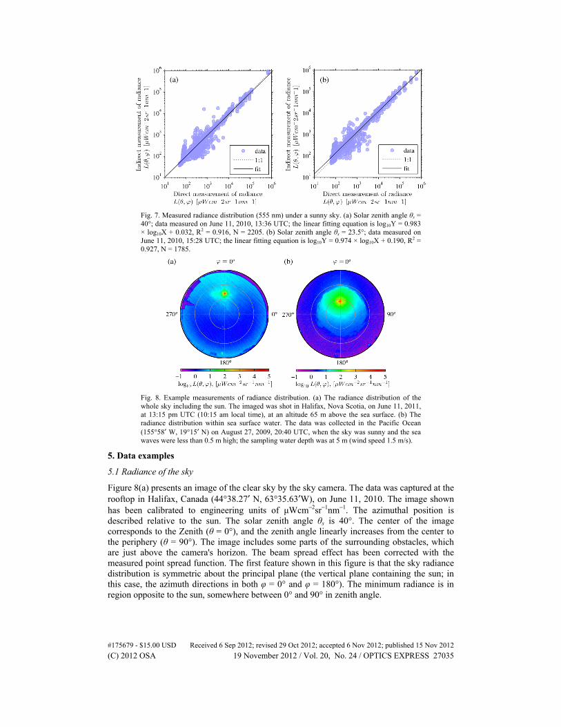
Fig. 7. Measured radiance distribution (555 nm) under a sunny sky. (a) Solar zenith angle θs = 40°; data measured on June 11, 2010, 13:36 UTC; the linear fitting equation is log10Y = 0.983 × log10X + 0.032, R2 = 0.916, N = 2205. (b) Solar zenith angle θs = 23.5°; data measured on June 11, 2010, 15:28 UTC; the linear fitting equation is log10Y = 0.974 × log10X + 0.190, R2 = 0.927, N = 1785.

Fig. 8. Example measurements of radiance distribution. (a) The radiance distribution of the whole sky including the sun. The imaged was shot in Halifax, Nova Scotia, on June 11, 2011, at 13:15 pm UTC (10:15 am local time), at an altitude 65 m above the sea surface. (b) The radiance distribution within sea surface water. The data was collected in the Pacific Ocean (155°58′ W, 19°15′ N) on August 27, 2009, 20:40 UTC, when the sky was sunny and the sea waves were less than 0.5 m high; the sampling water depth was at 5 m (wind speed 1.5 m/s).

5. Data examples

5.1 Radiance of the sky

Figure 8(a) presents an image of the clear sky by the sky camera. The data was captured at the rooftop in Halifax, Canada (44°38.27′ N, 63°35.63′W), on June 11, 2010. The image shown has been calibrated to engineering units of μWcm−2sr−1nm−1. The azimuthal position is described relative to the sun. The solar zenith angle θs is 40°. The center of the image corresponds to the Zenith (θ = 0°), and the zenith angle linearly increases from the center to the periphery (θ = 90°). The image includes some parts of the surrounding obstacles, which are just above the camera's horizon. The beam spread effect has been corrected with the measured point spread function. The first feature shown in this figure is that the sky radiance distribution is symmetric about the principal plane (the vertical plane containing the sun; in this case, the azimuth directions in both φ = 0° and φ = 180°). The minimum radiance is in region opposite to the sun, somewhere between 0° and 90° in zenith angle.


One inherent artifact with the full sky measurement is the lens flare induced by internal reflections and scattering in the lens and relay optics when imaging the sun. As shown in Fig. 8(a), the lens flare is most evident as several artefacts (bright dots) along the solar principal plane. The effect of lens flare is also significant in the circumsolar region (from 0.5° to ~10° relative to the sun). Reflection can also be seen at the bottom of the image.

Another potential problem, which is common for digital cameras, arises when the apparent image size of the object is larger than a pixel, such as the solar disk in our case. As a consequence, the image of the sun usually falls onto several neighbouring pixels instead of just one pixel. Since there is always one highest pixel value, we take the highest pixel as the radiance of the solar disk.

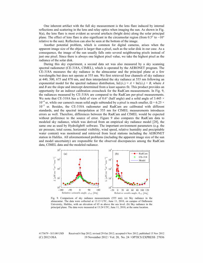
During this sky experiment, a second data set was also measured by a sky scanning spectral radiometer (CE-318A, CIMEL), which is operated by the AERONET program. The CE-318A measures the sky radiance in the almucantar and the principal plane at a few wavelengths but does not operate at 555 nm. We first retrieved four channels of sky radiance at 440, 500, 675 and 870 nm, and then interpolated the sky radiance at 555 nm following an exponential model for the spectral radiance distribution, lnL(λ1) = A × lnL(λ2) + B, where A and B are the slope and intercept determined from a least squares fit. This product provides an opportunity for an indirect calibration crosscheck for the RadCam measurements. In Fig. 9, the radiances measured by CE-318A are compared to the RadCam per-pixel measurements. We note that CE-318A has a field of view of 0.6° (half angle) and a solid angle of 3.445 × 10−4 sr, while our camera's mean solid angle subtended by a pixel is much smaller, Ω = 6.25 × 10−5 sr. Besides, the CE-318A radiometer and RadCam are calibrated with different standards, and the spectral interpolation at 555 nm for CIMEL measurements introduces errors as well. Therefore, differences between the RadCam and CIMEL would be expected without preference to the source of error. Figure 9 also compares the RadCam data to modeled sky radiance, which was derived from an empirical sky radiance model [28], the same one as used by Hydrolight® software. The important environment parameters (e.g. the air pressure, total ozone, horizontal visibility, wind speed, relative humidity and precipitable water content) was monitored and retrieved from local stations including the AERONET station in Halifax. All aforementioned problems (including the apparent image size of the sun and model uncertainty) are responsible for the observed discrepancies among the RadCam data, CIMEL data and the modeled radiance.

Fig. 9. Comparison of sky radiance measurements (555 nm). (a) Sky radiance in the almucantar. The data were collected at 13:15 UTC, June 11, 2010, on campus of Dalhousie University, Halifax, with an elevation of 65 m above the sea level. (b) Sky radiance in the principal plane. The data were measured at 13:24 UTC, June 11, 2010, at the same location.


Fig. 10. Comparison of the camera measurements with the OCR-504 radiometer measurements (555 nm) under sunny skies. (a) Example depth profiles of the downwelling plane irradiance Ed. (b) Example depth profiles of the upwelling nadir radiance Lu. (c) Scatter plots of the downwelling plane irradiance retrieved from measured depth profiles; the best fit is given as log10Y = 0.992 × log10X + 0.009, R2 = 0.938, N = 2189. (d) Scatter plots of the upwelling nadir radiance from retrieved depth profiles; the best fit is log10Y = 1.025 × log10X + 0.006, R2 = 0.990, N = 2211.These data were collected from surface down to 40 m in Pacific Ocean off the Big Island of Hawaii, during August 27 to September 14, 2010.

5.2 Radiance in the sea

Example measurements for the full radiance distribution offshore of Hawaii are given in Fig. 8(b). The sky was sunny but slightly hazy. For the underwater radiance image, we rarely observe obvious lens flare as in above-water applications. That is because the radiance of the refracted sun underwater is often attenuated relative to the sun in the air, and the sea water has a larger refractive index than the air which further reduces the surface reflection upon the window. For this example, the downwelling radiance field spans up to 6 orders of magnitude. The upwelling radiance field varies within one order of magnitude (figure not shown).

The OCR-504I/R measures the irradiance and radiance at wavelengths identical to the RadCam. Figure 10(a) illustrates the downwelling irradiance profiles measured by two sensors in the Pacific Ocean and under sunny skies and shows no significant difference in the wave-induced fluctuations. The fluctuations seen in Fig. 10(b) are mainly caused by the sensor inclinations. The camera measurements are quantitatively compared with OCR-504 data in Fig. 10(c) and Fig. 10(d), each of which is composed of more than 2000 data points collected in different locations in the Pacific Ocean. The observed difference is less than measured in the lab: SMAPDs are 14.2% for the irradiance data and 6.2% for the upwelling radiances. We note that these estimated differences have included both the measurement uncertainty and the variance of the spatial distribution of the light field as influenced by sea waves. As the wave focusing effect is more significant for the downwelling light than the


upwelling light distribution [e.g [29].], the real measurement uncertainties for downwelling plane irradiance and upwelling nadir radiance are likely smaller than 14% and 6% respectively.

6. Discussion and summary

To the best of our knowledge, RadCam is the first imaging radiometer capable of a response spanning over 6 orders of magnitude in a given scene and up to 9 orders with changes in exposure. The high dynamic range measuring capability permits the mapping of the full 4π radiance field in the near-surface water environment. And the new camera can operate at a faster rate, up to 15 Hz, than existing oceanographic radiance camera systems [e.g 16.]. This development of high dynamic range radiance camera system represents a fundamental improvement to the radiometry of in-water optical measurements.

Based on the data comparison made in the lab and field, good agreement has been achieved between the RadCam measurements and other reference instruments with an average difference of 14%-16% over the wide dynamic range (Fig. 6 and Fig. 10). Uncertainties in the light source, non-linear high dynamic range response functions, immersion factor, point spread function and the nonuniform spectral response over the 20-nm bandwidth all contribute to the combined uncertainty. Among them, the high dynamic range response functions are the hardcore in the instrument development and are probably the principal contributor to the total uncertainty. The upwelling radiance measurement was always collected with low-exposure settings, which showed a small uncertainty of only 6%-10%.

The high dynamic range, geometrically and radiometrically accurate, and multi-angular imaging system provides new possibilities for applications of hydrologic optics. For example, it can be readily deployed to measure the light field at clam or high seas. Data can be directly used for ocean optical modeling and quantification of the optical properties of the water [1]. The simultaneous measurement of the sky (plus the sun) radiance distribution allows the evaluation of the influence of both the sea-surface roughness and in-water inherent optical properties in shaping the evolution of the radiance distribution with depth.

The newly developed instrument has also shown excellent potential for atmospheric monitoring. In particular, the un-occluded camera system can be employed for all-sky (including the sun) radiance mapping in absolute scales. Such data are requisite in atmospheric radiative transfer modelling, solar radiation, lighting condition and cloudiness monitoring, etc.

We anticipate that the sensor development will continue for improvement of the measurement accuracy. A future design may also consider multi-spectral resolving capability. Related data processing algorithms are worth investigating as well, in particular, for the high dynamic range image deblurring.

Acknowledgments

The authors would like to acknowledge support from the Office of Naval Research (N00014-04-C-0132, N00014-07-C0139, and N00014-09-C-0084) for the development of RadCam and for field trials as part of the Radiance in a Dynamic Ocean (RaDyO) program. The MITACS Accelerate PhD Fellowship program provided support to Jianwei Wei during 2011-2012. Dr. Glen Lesins provided assistance in the CIMEL sky radiance measurement. The authors are grateful to two anonymous reviewers for their comments and suggestions.


Documents

A new instrument for measuring the high dynamic range ...rads.physics.miami.edu/optics/ken/RefPapers/079_WDLMV_OE_2012.pdf · A new instrument for measuring the high dynamic range