A NEW BEHAVIOR OF CHAOTIC ATTRACTORS

Nahed AOUF, Nader.BELGITH, Kais.BOUALLEGUE, Mohsen MACHOUT1Department Electronic and Micro-Electronic Laboratory, Faculty of Sciences of

Monastir, University of Monastir 5000, Tunisia.(E-mail: nahedaouf@gmail.com)

2Department of Electrical Engineering, Higher Institute of Applied Sciences andTechnology of Sousse, University of Sousse, Tunisia.

Cite Taffala ( ISSAT ), 4003 Sousse Tunisie,

Abstract

This paper presents a new behavior of chaotic attractor. Therefore,creatinga chaotic attractor with bounded behavior is a theoretically very attractiveand yet technically a quite challenging task.It is obviously significant to cre-ate more complicated multi chaotic attractor with bounded behavior, in boththeory and engineering application. Simulation demonstrates the validity andfeasibility of the proposed method.

Keywords: Chua attractor, Rossler attractor, bounded function with bounded sup-port,bounded function with compact support.

1 Introduction

The behavior of chaotic attractor is very interesting nonlinear effect which hasbeen competently studied during the last four decades [1]. It reaches many naturaland artificial dynamic systems such as human heart, mechanical system, electroniccircuits, etc [2]. There are so many classical attractors are known until now suchus Lorenz , Rossler , Chua , Chen, and others... Our approach in this paper is togenerate a new behavior of chaotic attractor using Chua attractor and Julia Process.

2 Julia’s Process

In recent years, there have been a lot of developments in Julia sets, including qual-itative characters, applications and controls. In this section, the use of algorithmsinspired from Julia processes, will be presented. To generate Julia processes, someof the properties are well known:

• The Julia set is a repeller.

551

• The Julia set is invariant.

• An orbit on Julia set is either periodic or chaotic.

• All unstable periodic points are on Julia set.

• The Julia set is either wholly connected or wholly disconnected.

• All sets generated only with Julia sets combination has fractal structure[5].

Real and imaginary parts of the complex numbers are separately calculated.xi+1 = x2

i − y2i + xc

yi+1 = xiyi + yc(1)

The listing of algorithm P is as follows:

Algorithm 1 (yi+1, xi+1) = P (arctan(xi), yi)1: if xi < 0 then2: xi+1 =

√(√

((arctan(xi))2 + (yi)2) + arctan(xi)2 )

3: yi+1 = yi2xi+1

4: end if5: if xi = 0 then6: xi+1 =

√|yi|2

7: if xi > 0 then8: xi+1 = yi

2yi+19: end if

10: if xi < 0 then11: yi+1 = 012: end if13: end if14: if xi > 0 then15: yi+1 =

√(√

((arctan(xi))2 + (yi)2)− arctan(xi)2 )

16: xi+1 = yi2xi+1

17: if yi < 0 then18: yi+1 = −yi+119: end if20: end if

552

3 Rossler attractor

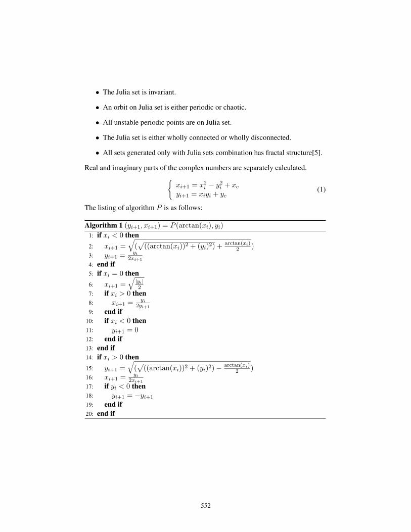
Rossler system was introduced in the 1970s as prototype equation with the mini-mum ingredients for continuous time chaos. This system is minimal for continuouschaos for at least three reasons: Its phase space has the minimal dimension three,its nonlinearity is minimal because there is a single quadratic term, and it generatesa chaotic attractor with a single scroll, in contrast to the Lorenz attractor with hastwo scrolls.

M

z1 = −(z2 + z3)z2 = z1 + αz2z3 = (z1z3 − βz3 + γz1)

(2)

(a)

Figure 1: Rossler chaotic attractor

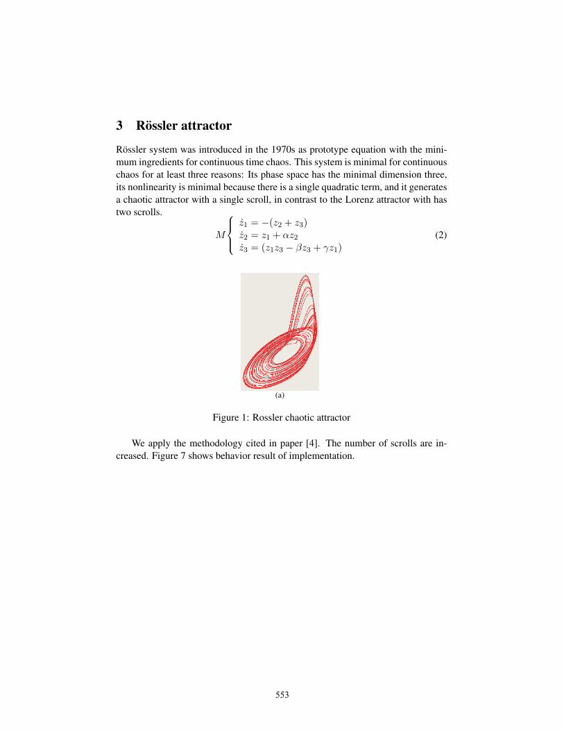
We apply the methodology cited in paper [4]. The number of scrolls are in-creased. Figure 7 shows behavior result of implementation.

553

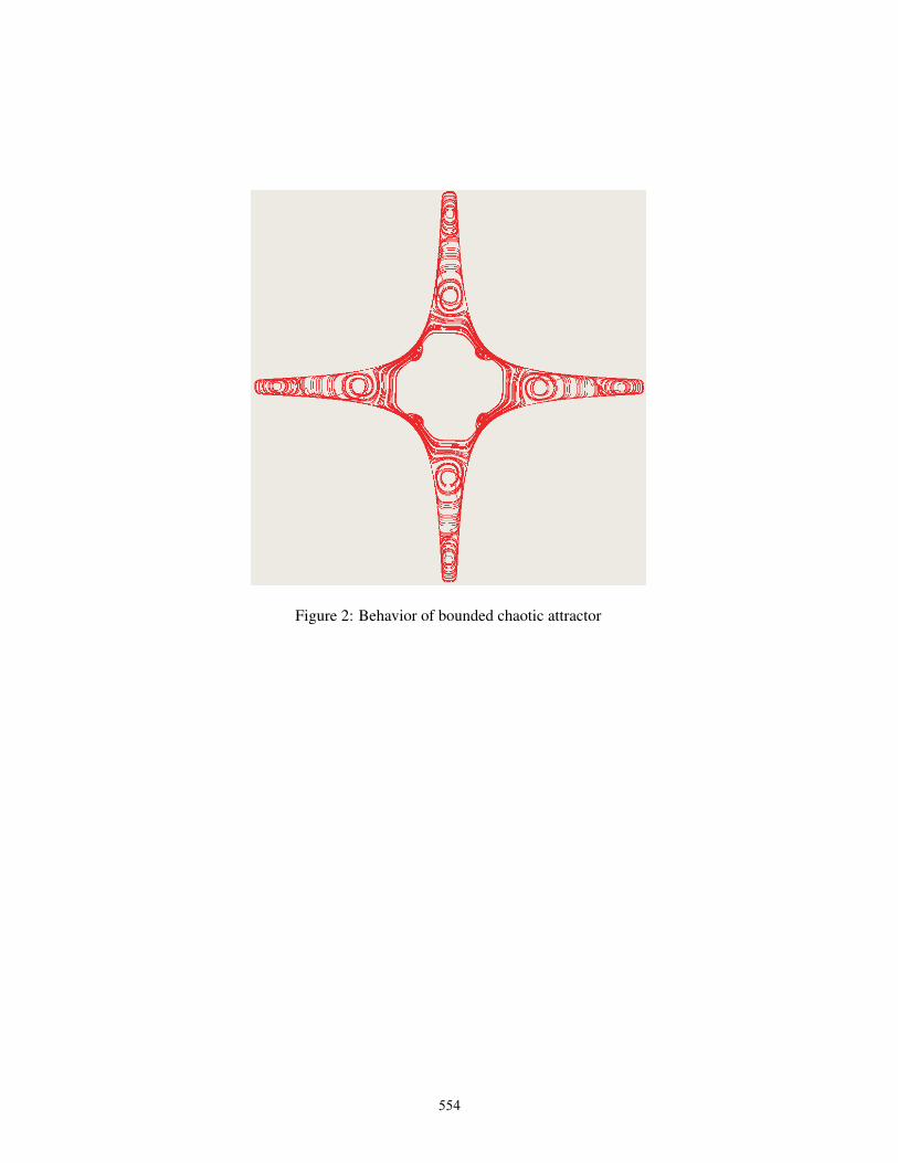
Figure 2: Behavior of bounded chaotic attractor

554

Figure 3: An other behavior of bounded chaotic attractor

555

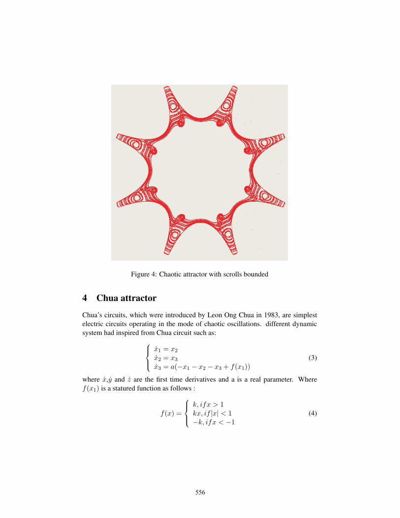
Figure 4: Chaotic attractor with scrolls bounded

4 Chua attractor

Chua’s circuits, which were introduced by Leon Ong Chua in 1983, are simplestelectric circuits operating in the mode of chaotic oscillations. different dynamicsystem had inspired from Chua circuit such as:

x1 = x2x2 = x3x3 = a(−x1 − x2 − x3 + f(x1))

(3)

where x,y and z are the first time derivatives and a is a real parameter. Wheref(x1) is a statured function as follows :

f(x) =

k, ifx > 1kx, if |x| < 1−k, ifx < −1

(4)

556

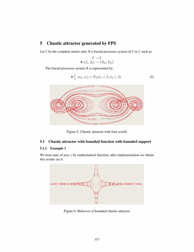
5 Chaotic attractor generated by FPS

Let E be the complete metric unit, Φ a fractal processes system of E in E such as:

E→ E

Φ:(f1, f2)→ (XG, YG)

The fractal processes system Φ is represented by:

Φ

(u1, v1) = PJ(x1 + β, x2 + β) (5)

Figure 5: Chaotic attractor with four scrolls

5.1 Chaotic attractor with bounded function with bounded support

5.1.1 Example 1

We treat state of axis x by mathematical function, after implementation we obtainthis results see 6.

Figure 6: Behavior of bounded chaotic attractor

557

via changing the value of β the behavior of bounded chaotic attractor changed.

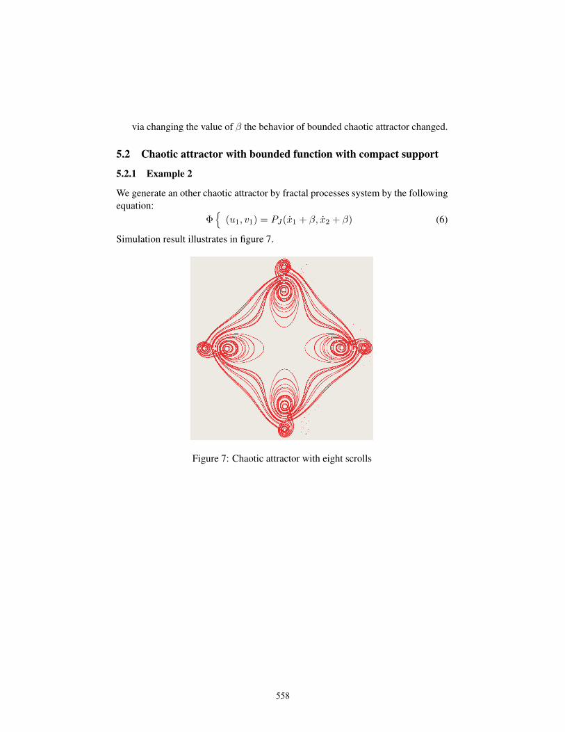
5.2 Chaotic attractor with bounded function with compact support

5.2.1 Example 2

We generate an other chaotic attractor by fractal processes system by the followingequation:

Φ

(u1, v1) = PJ(x1 + β, x2 + β) (6)

Simulation result illustrates in figure 7.

Figure 7: Chaotic attractor with eight scrolls

558

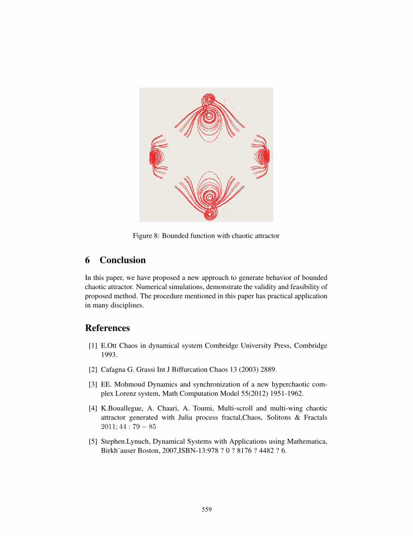
Figure 8: Bounded function with chaotic attractor

6 Conclusion

In this paper, we have proposed a new approach to generate behavior of boundedchaotic attractor. Numerical simulations, demonstrate the validity and feasibility ofproposed method. The procedure mentioned in this paper has practical applicationin many disciplines.

References

[1] E.Ott Chaos in dynamical system Combridge University Press, Combridge1993.

[2] Cafagna G. Grassi Int J Biffurcation Chaos 13 (2003) 2889.

[3] EE. Mohmoud Dynamics and synchronization of a new hyperchaotic com-plex Lorenz system, Math Computation Model 55(2012) 1951-1962.

[4] K.Bouallegue, A. Chaari, A. Toumi, Multi-scroll and multi-wing chaoticattractor generated with Julia process fractal,Chaos, Solitons & Fractals2011; 44 : 79− 85

[5] Stephen.Lynuch, Dynamical Systems with Applications using Mathematica,Birkh¨auser Boston, 2007,ISBN-13:978 ? 0 ? 8176 ? 4482 ? 6.

559

560

HYPERCHAOS SET BY FRACTAL PROCESSES SYSTEMSalah NASR1,+,Nahed AOUF2, Kais BOUALLEGUE3,Hassen MEKKI4,Mohsen Machhout 2.

1

1+CEM Lab, National Engineering School of Sfax, BP-1173, 3038 Sfax, Tunisia2Department Electronic and Micro-Electronic Laboratory, Faculty of Sciences of Monastir, university ofMonastir 5000, Tunisia. 3Department of Electrical Engineering. Higher Institute of Applied Sciences and

Technology of Sousse, Tunisia4 National Engineering School of Sousse, Sousse, Tunisia

Abstract.This paper presents a new class of hyper chaotic attractor. This hyperchaos is a set of chaoticattractors with different number of scrolls. It has different behavior forms either separated ornot with or without other nested chaotic attractors. This class of systems is constructed by us-ing fractal processes system (FPS). For each parameter value which is treated by process thatis presented in the FPS generates a new behavior and increases the number of scrolls. There-fore,creating a multi chaotic attractors with nested ones is a theoretically very attractive and yettechnically a quite challenging task.It is obviously significant to create more complicated multichaotic attractor and multi hyper-chaotic attractor, in both theory and engineering application.Simulation demonstrates the validity and feasibility of the proposed method.

Keywords: Multi-chaotic attractor, hyper chaotic attractor, fractal processes.

1 Introduction

Chaotic system has became a popular research area around the world after the first three-dimensional chaoticsystem was discovered by Lorenz, and many new chaotic systems have been proposed (i.e., Chen system,Lu system, Liu system)[3]

Recently, exploiting chaotic dynamics in high-tech and industrial engineering applications has attractedmuch interest, wherein more attention has been focused on creating chaos effectively[4].

Compared with the simple chaotic attractors, multi chaotic attractors can provide more complex dynamicbehaviors, more adjustability and more encryption parameters. These properties indicate that multi- chaoticattractors have a general potential applications to communications, cryptography and many other fields.

Many methods have been used to construct a hyperchaotic system and several hyper chaotic have beendiscovered in high dimensional dynamics such as Hyperchaotic Rossler system [6], hyperchaotic Chua’scircuit [7] and hyperchaotic Lorenz system [8]. Our approach is regarded as a new class of hyper chaos.

The rest of the paper is organized as follows: In section 2, We describe generation of multi chaoticattractors separated and non separated with the same behavior. In section 3 introduce an another generationof multi chaotic attractors with different form of behavior.

Finally ,in section 4 we conclude this paper by providing a summary of the above finding.

2 Chaos with the same form of behavior

We recall the structure of fractal processes system described in paper [10]. Here, we present a structure of asystem of fractal processes by associating multiple fractal processes in a cascading manner. This structurestarts with a set of initial conditions, a number of fractal processes, and a set of transformations.

Let E be the complete metric unit, Φ a system of fractal processes in E such as:

E→ E

Φ:(xi, yi)→ (xm, ym)1 Corresponding author

E-mail address: nasrsalah-tun@hotmail.fr

_________________

8th CHAOS Conference Proceedings, 26-29 May 2015

Henri Poincaré Institute, Paris France

© 2015 ISAST

561

The fractal processes system Φ is represented by:

Φ

(x0, y0)(xi+1, yi+1) = P1(αxi + γ, βyi + λ)(xi+2, yi+2) = P2(xi+1, yk+1)(xi+3, yi+3) = T1(xi+2, yi+2)(xi+4, yi+4) = P3(xi+3, yi+3)...(xj+1, yj+1) = Tk(xj−1, yj−1)...(xm, ym) = Pm−k(xm−1, ym−1)

(1)

The dynamics of the system of fractal processes is controlled by the assignment of xi+1 to xi and of yi+1 toyi.

xi ← xi+1yi ← yi+1

(2)

The system (1) is a combination of different transformations and different processes. It consists of mequations and k transformations, so m− k processes for n iterations where the first iteration is (x0, y0).

We give different examples using FPS to show and validate our approach.

2.1 Chaos with separated chaotic attractors

In this paper, we use two classical chaotic attractors the first one we take Lorenz attractor in the second wechoose Chua attractor. We recall the structure of the two chaotic attractors.

The Lorenz system [2]has become one of paradigms in the research of chaos, and is described by wherex1, x2 and x3 are system states and σ, ρ and β

M

z1 = σ(z2 − z1)z2 = ρz1 − z2 − z1z3z3 = (z1z2 − βz3)

(3)

And the second is Chua’s circuits[?], which were introduced by Leon Ong Chua in 1983, are simplestelectric circuits operating in the mode of chaotic oscillations. different dynamic system had inspired fromChua circuit such as:

x1 = x2x2 = x3x3 = a(−x1 − x2 − x3 + f(x1))

(4)

where y1,y2 and y3 are the first time derivatives and a is a real parameter. Where f(y1) is a statured functionas follows :

f(x) =

k, ifx > 1kx, if |x| < 1−k, ifx < −1

(5)

2.2 Chaos with same behavior of separated chaotic attractors

Consider the following Φ a fractal processes system :Let E be the complete metric unit, Φ a fractal processes system of E in E such as:

E→ E

Φ:(f1, f2)→ (XG, YG)

562

The fractal processes system Φ is represented by:

Φ

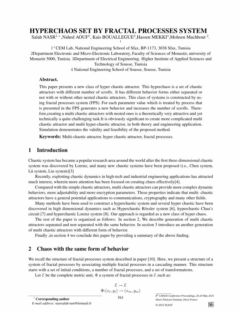
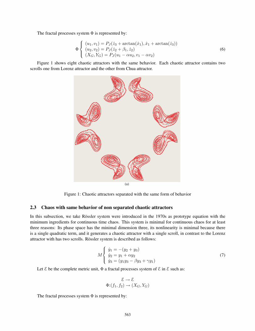
(u1, v1) = PJ(z3 + arctan(x1), x1 + arctan(z3))(u2, v2) = PJ(z2 + β1, z2)(XG, YG) = PJ(u1 − αu2, v1 − αv2)

(6)

Figure 1 shows eight chaotic attractors with the same behavior. Each chaotic attractor contains twoscrolls one from Lorenz attractor and the other from Chua attractor.

(a)

Figure 1: Chaotic attractors separated with the same form of behavior

2.3 Chaos with same behavior of non separated chaotic attractors

In this subsection, we take Rossler system were introduced in the 1970s as prototype equation with theminimum ingredients for continuous time chaos. This system is minimal for continuous chaos for at leastthree reasons: Its phase space has the minimal dimension three, its nonlinearity is minimal because thereis a single quadratic term, and it generates a chaotic attractor with a single scroll, in contrast to the Lorenzattractor with has two scrolls. Rossler system is described as follows:

M

y1 = −(y2 + y3)y2 = y1 + αy2y3 = (y1y3 − βy3 + γy1)

(7)

Let E be the complete metric unit, Φ a fractal processes system of E in E such as:

E→ E

Φ:(f1, f2)→ (XG, YG)

The fractal processes system Φ is represented by:

563

Φ

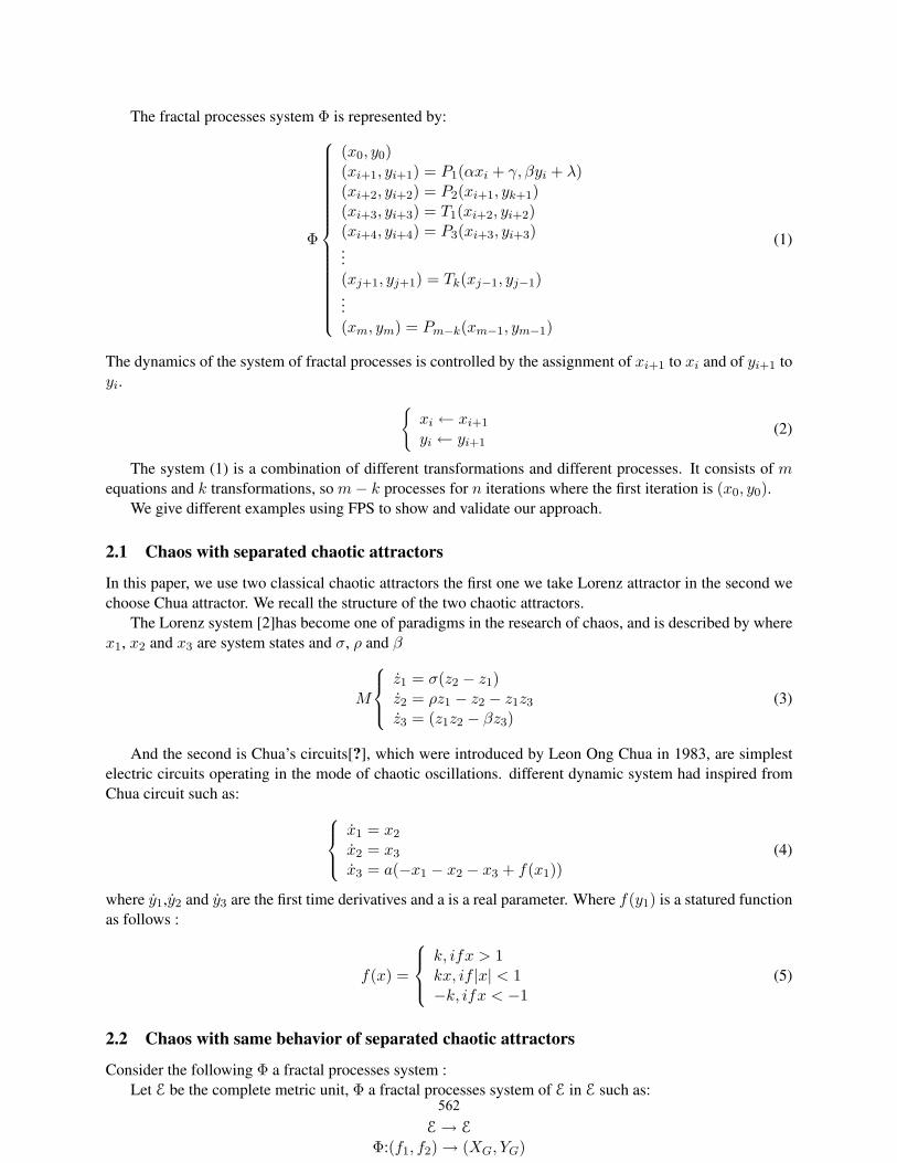
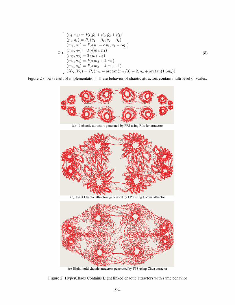
(u1, v1) = PJ(y1 + β1, y2 + β2)(p1, q1) = PJ(y1 − β1, y2 − β2)(m1, n1) = PJ(u1 − αp1, v1 − αq1)(m2, n2) = PJ(m1, n1)(m3, n3) = T (m2, n2)(m4, n4) = PJ(m3 + 4, n3)(m5, n5) = PJ(m3 − 4, n3 + 1)(XG, YG) = PJ(m4 − arctan(m5/3) + 2, n4 + arctan(1.5n5))

(8)

Figure 2 shows result of implementation. These behavior of chaotic attractors contain multi level of scales.

(a) 16 chaotic attractors generated by FPS using Rossler attractors

(b) Eight Chaotic attractors generated by FPS using Lorenz attractor

(c) Eight multi chaotic attractors generated by FPS using Chua attractor

Figure 2: HyperChaos Contains Eight linked chaotic attractors with same behavior

564

3 Chaos with the different form of behavior

3.1 Chaos with two behavior of chaotic attractors

A new chaotic attractors with two forms of behavior is established by the following Fractal Processes Sys-tem:

Let E be the complete metric unit, Φ a fractal processes system of E in E such as:

E→ E

Φ:(f1, f2)→ (XG, YG)

The fractal processes system Φ is represented by:

Φ

(u1, v1) = PJ(x1 + arctan(x1), x2 + arctan(x2))(u2, v2) = (1− u1, 1− v1)(p1, q1) = PJ(z2 + β, z3 − β)(p2, q2) = (α1p1(1− p1), α2q1(1− q1))(m1, n1) = PJ(u1 − p1, v1 − q1)(r1, s1) = PJ(x1 − β1, x2 − β2)(XG, YG) = PJ(r1 − ρm1 + λ, s1 − ρn1)

(9)

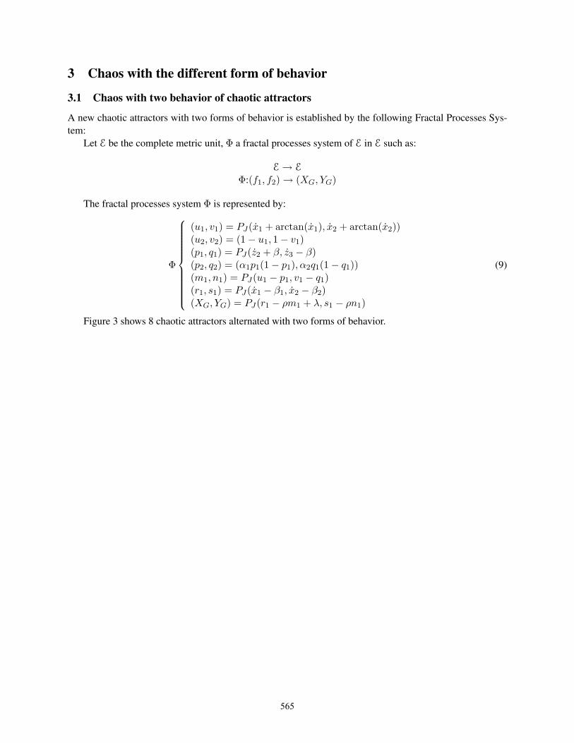
Figure 3 shows 8 chaotic attractors alternated with two forms of behavior.

565

(a) 8 chaotic attractors separated

(b) First behavior chaotic attractors (c) Second behavior chaotic attractors

Figure 3: Chaos with two behavior of chaotic attractors

3.2 Chaos with three behavior of chaotic attractors with four times

Let E be the complete metric unit, Φ a fractal processes system of E in E such as:

E→ E

Φ:(f1, f2)→ (XG, YG)

The fractal processes system Φ is represented by:

Φ

(u1, v1) = PJ(x1 + arctan(x1), x2 + arctan(x2))(u2, v2) = PJ(z2 + β1, z3)(u3, v3) = PJ(u1 − 2u2 + β2, v1 − v2)(p1, q1) = PJ(z2 + β3, z3)(p2, q2) = PJ(u1 − 2p1, v1 − q1)(XG, YG) = PJ(u3 − 2p2, v3 − 2q2)

(10)566

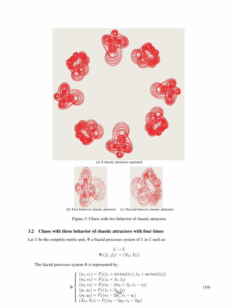
Fractal processes system contains two different chaotic attractors the first one we choose Chua attractornoted with x the other Lorenz attractor noted with z. Implementation of fractal processes system showsresult in figure

Figure 4 shows the result of implementation, It contains multi chaotic attractors with fractal and multifractal scrolls.

(a)

Figure 4: Chaotic attractors with three forms of behavior

Figure5 illustrates the three forms of behavior of chaotic attractors with fractal scrolls.

(a) First form of behavior(b) Second form of behavior (c) Third form of behavior

Figure 5: Three forms of behavior of chaotic attractors

3.3 Chaos with nested and three behavior of chaotic attractors

Let E be the complete metric unit, Φ a fractal processes system of E in E such as:

E→ E

Φ:(f1, f2)→ (XG, YG)

The fractal processes system Φ is represented by:

567

Φ

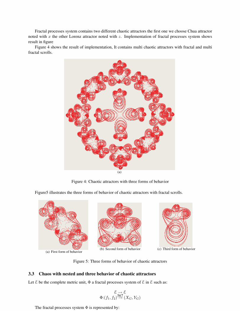
(u1, v1) = PJ(x1 + arctan(x1), x2 + arctan(x2))(u2, v2) = PJ(z2 + β1, z3 − β)(u3, v3) = PJ(u1 − αu2 + β2, v1 − v2)(p1, q1) = PJ(z2 + β3, z3)(p2, q2) = PJ(u1 − αp1, v1 − q1)(XG, YG) = PJ(u3 − 2p2, v3 − 2q2)

(11)

(a)

Figure 6: Chaotic attractors separated within nested chaotic attractors

3.4 Chaos with four behavior of chaotic attractors

Let E be the complete metric unit, Φ a fractal processes system of E in E such as:

E→ E

Φ:(f1, f2)→ (XG, YG)

The fractal processes system Φ is represented by:

Φ

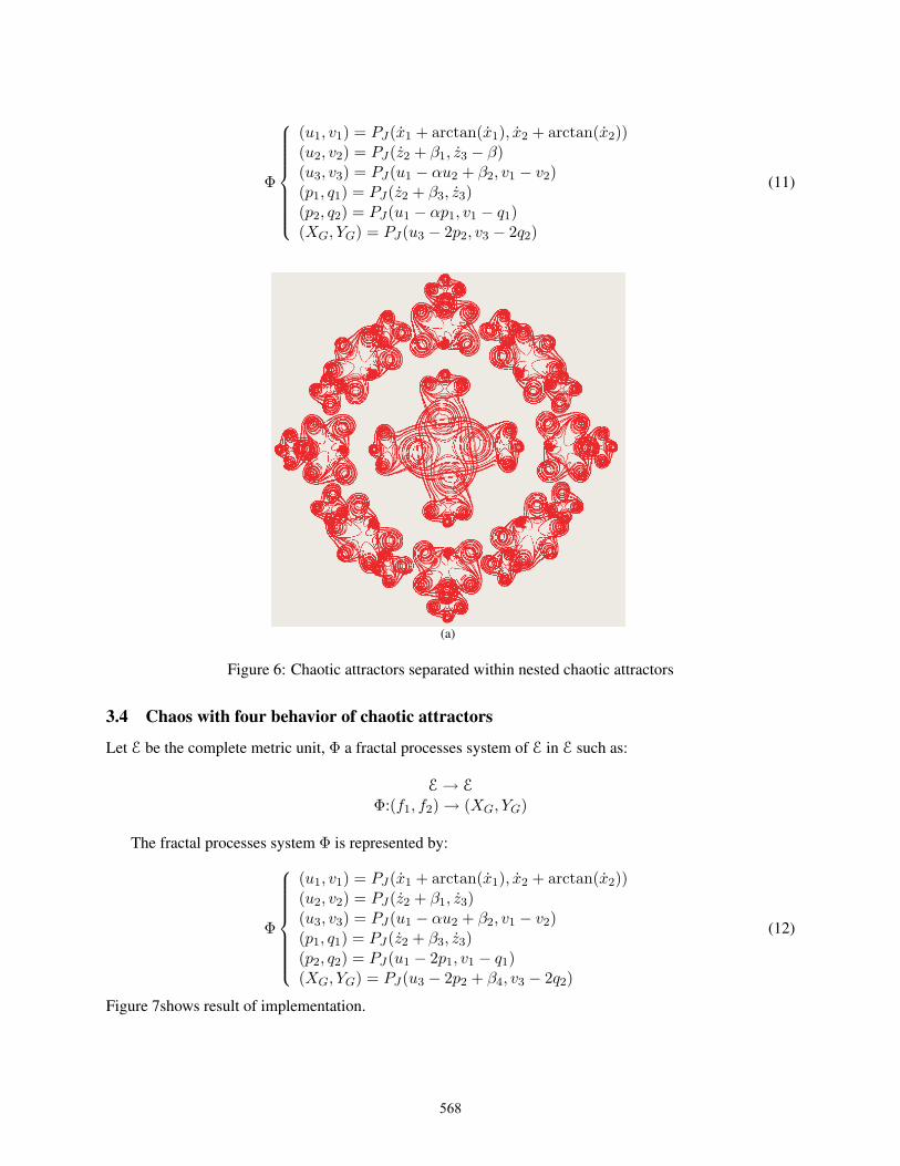
(u1, v1) = PJ(x1 + arctan(x1), x2 + arctan(x2))(u2, v2) = PJ(z2 + β1, z3)(u3, v3) = PJ(u1 − αu2 + β2, v1 − v2)(p1, q1) = PJ(z2 + β3, z3)(p2, q2) = PJ(u1 − 2p1, v1 − q1)(XG, YG) = PJ(u3 − 2p2 + β4, v3 − 2q2)

(12)

Figure 7shows result of implementation.

568

(a)

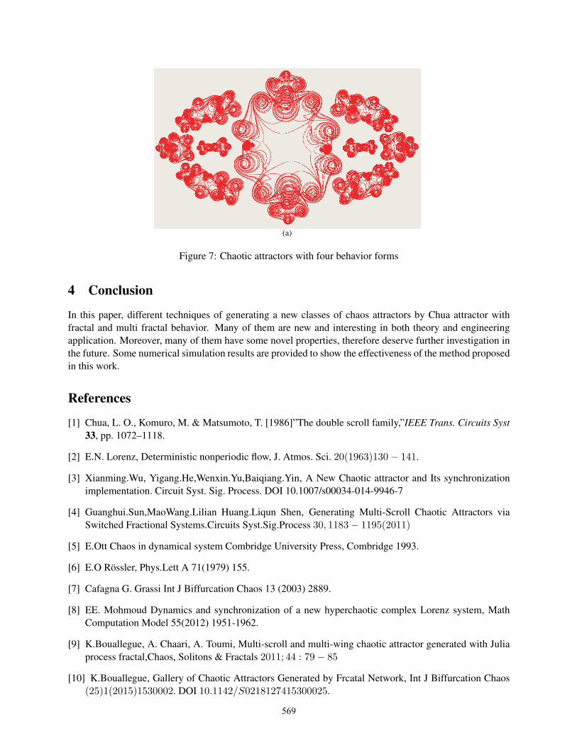
Figure 7: Chaotic attractors with four behavior forms

4 Conclusion

In this paper, different techniques of generating a new classes of chaos attractors by Chua attractor withfractal and multi fractal behavior. Many of them are new and interesting in both theory and engineeringapplication. Moreover, many of them have some novel properties, therefore deserve further investigation inthe future. Some numerical simulation results are provided to show the effectiveness of the method proposedin this work.

References

[1] Chua, L. O., Komuro, M. & Matsumoto, T. [1986]”The double scroll family,”IEEE Trans. Circuits Syst33, pp. 1072–1118.

[2] E.N. Lorenz, Deterministic nonperiodic flow, J. Atmos. Sci. 20(1963)130− 141.

[3] Xianming.Wu, Yigang.He,Wenxin.Yu,Baiqiang.Yin, A New Chaotic attractor and Its synchronizationimplementation. Circuit Syst. Sig. Process. DOI 10.1007/s00034-014-9946-7

[4] Guanghui.Sun,MaoWang.Lilian Huang.Liqun Shen, Generating Multi-Scroll Chaotic Attractors viaSwitched Fractional Systems.Circuits Syst.Sig.Process 30, 1183− 1195(2011)

[5] E.Ott Chaos in dynamical system Combridge University Press, Combridge 1993.

[6] E.O Rossler, Phys.Lett A 71(1979) 155.

[7] Cafagna G. Grassi Int J Biffurcation Chaos 13 (2003) 2889.

[8] EE. Mohmoud Dynamics and synchronization of a new hyperchaotic complex Lorenz system, MathComputation Model 55(2012) 1951-1962.

[9] K.Bouallegue, A. Chaari, A. Toumi, Multi-scroll and multi-wing chaotic attractor generated with Juliaprocess fractal,Chaos, Solitons & Fractals 2011; 44 : 79− 85

[10] K.Bouallegue, Gallery of Chaotic Attractors Generated by Frcatal Network, Int J Biffurcation Chaos(25)1(2015)1530002. DOI 10.1142/S0218127415300025.

569

570

_________________

8th

CHAOS Conference Proceedings, 26-29 May 2015, Henri Poincaré Institute, Paris France

© 2015 ISAST

Statistics of Chaos

David C. Ni

Dept. of Mathematical Research, Direxion Technology

9F, No. 177-1, Ho-Ping East Rd., Sec 1, Daan District, Taipei, Taiwan, R.O.C.

Abstract. In a previous effort, we demonstrated that transition to chaos being related to

symmetry broken of the divergent sets in fractal forms of complex momentum-and-

angular-momentum plane, which are constructed by an extended Blaschke product

(EBP).

In the recent efforts, we demonstrated root computation via iteration of EBP. Using

newly developed algorithms, we iterate the EBP and have mapped the convergent sets in

the domains to the disconnected solution sets in the codomains. We demonstrated that

solution sets showing various forms of canonical distributions and found counter

examples of Fundamental Theorem of Algebra (FTA).

In this paper, we further extend the root-computation algorithms to the transition regions

of chaos in the domains and the mapped codomains. We characterize the solution sets

and explore the methodologies and the related theories to the modelling of physical

phenomena, such as formation of galaxy cluster and stellar system.

Keywords: Nonlinear Lorentz Transformation, Nonlinear Relativity, Blaschke Equation,

Fractal, Iterated solutions, Chaos, Statistics, dynamical systems.

1 Introduction

Contemporary models for N-body systems are mainly extended from temporal,

two-body, and mass point representation of Newtonian mechanics. Other

mainstream models include 2D/3D Ising models constructed from the lattice

structures. These models have been encountering on-going debates in statistics.

We were motivated to develop a new construction directly from complex-

variable N-body systems based on the extended Blaschke functions (EBF)[1],

which represent a non-temporal and nonlinear extension of Lorentz

transformation on the complex plane – the normalized momentum-angular-

momentum space. A point on the complex plane represents a normalized state of

momentum and angular momentum (or phase) observed from a reference frame

in the context of the theory of special relativity. This nonlinear representation

couples momentum and angular momentum through real-imaginary equation of

complex number.

571

The limited convergent sets in the domains and the corresponding codomains

demonstrated hierarchical structures and topological transitions depending on

parameter space. Among the transitions, continuum-to-discreteness transitions,

nonlinear-to-linear transitions, and phase transitions manifest this construction

embedded with structural richness for modelling broad categories of physical

phenomena. In addition, we have recently developed a set of new algorithms for

solving EBF iteratively in the context of dynamical systems. The solution sets

generally follow the Fundamental Theorem of Algebra (FTA), however,

exceptional cases are also identified. Through iteration, the solution sets show a

form of σ + i [-t, t], where σ and t are the real numbers, and the [-t, t] shows

canonical distributions.

As in the previous paper [2,3,4,5,6,7], we introduce an angular momentum to

the EBF, and for the degree of EBF, n, is greater than 2, we observed that the

fractal patterns showing lags as shown in Fig. 9(a). As angular momentum

increases, the divergent sets (fractal patterns) are connected to the adjacent sets

and diffuse as shown in Fig. 9(a). As iteration further increasing, subsequently

all convergent sets will become null set, which we define as chaotic state in this

paper. The main effort hereby is to extend the solution iteration algorithm to the

transition regions, where the domains and codomains becoming chaotic state.

Particularly, we characterize the convergent sets in the codomain near the

chaotic transition. The related theories and methodologies manifest a new

paradigm for modeling chaos. As an example of efforts on the applications of

modeling the physical phenomena, we apply the observations to the theories of

formation of galaxy clusters and stellar systems.

2 Construction of functions and equations

2.1. Functions and Equations

Given two inertial frames with different momentums, u and v, the observed

momentum, u’, from v-frame is as follows:

u’ = ( u - v ) / ( 1 - vu/c2 ) (1)

We set c2 = 1 and then multiply a phase connection, exp(iψ(u)), to the

normalized complex form of the equation (1) to obtain the following:

(u’/u) = exp(iψ(u))(1/u)[(u-v)/(1-uv)] (2)

We hereby define a generalized complex function as follows:

fB,(z,m)= z-1

ΠmCi

(3)

And Ci has the following forms:

572

Ci = exp(gi(z))[(ai-z)/( 1-āiz)] (4)

Where z is a complex variable representing the momentum u, ai is a parameter

representing momentum v, āi is the complex conjugate of a complex number ai

and m is an integer. The term gi(z) is a complex function assigned to Σp2pπiz

with p as an integer. The degree of fB(z,m) = P(z)/Q(z) is defined as Maxdeg P,

deg Q. The function fB is called an extended Blaschke function (EBF). The

extended Blaschke equation (EBE) is defined as follows:

fB(z,m) – z = 0 (5)

2.2. Domains and Codomains

A domain can be the entire complex plane, C∞, or a set of complex numbers,

such as z = x+yi, with (x2

+y2)1/2 ≦ R, and R is a real number. For solving the

EBF and EBE, a function f will be iterated as:

f n(z) = f f

n-1(z), (6)

Where n is a positive integer indicating the number of iteration. The function

operates on a domain, called domain. The set of f n(z) is called mapped

codomain or simply a codomain. In the figures, the regions in black color

represent stable Fatou sets containing the convergent sets of the concerned

equations and the white (i.e., blank) regions correspond to Julia sets containing

the divergent sets, the complementary sets of Fatou sets on C∞ in the context of

dynamical systems.

2.3. Parameter Space

In order to characterize the domains and codomains, we define a set of

parameters called parameter space. The parameter space includes six parameters:

1) z, 2) a, 3) exp(gi(z)), 4) m, 5) iteration, and 6) degree. In the context of this

paper we use the set z, a, exp(gi(z)), m, iteration, degree to represent this

parameter space. For example, a, is one of the subsets of the parameter space.

2.4. Domain-Codomain Mapping

On the complex plane, the convergent domains of the EBFs form fractal patterns

of with limited-layered structures (i.e., Herman rings), which demonstrate skip-

symmetry, symmetry broken, chaos, and degeneracy in conjunction with

parameter space [7]. Fig. 1 shows a circle in the domain is mapped to a set of

twisted figures in the codomain. We deduce that the mapping related to the tori

structures in conjunction with EBFs.

573

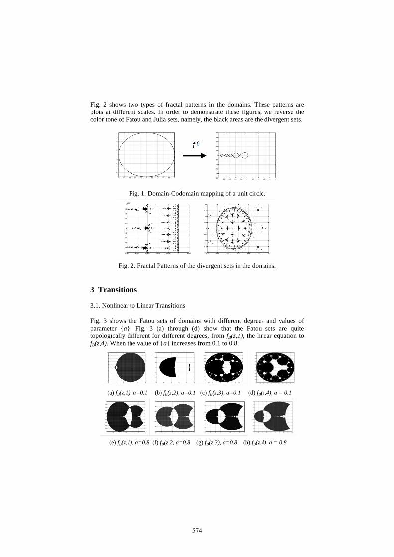
Fig. 2 shows two types of fractal patterns in the domains. These patterns are

plots at different scales. In order to demonstrate these figures, we reverse the

color tone of Fatou and Julia sets, namely, the black areas are the divergent sets.

Fig. 1. Domain-Codomain mapping of a unit circle.

Fig. 2. Fractal Patterns of the divergent sets in the domains.

3 Transitions

3.1. Nonlinear to Linear Transitions

Fig. 3 shows the Fatou sets of domains with different degrees and values of

parameter a. Fig. 3 (a) through (d) show that the Fatou sets are quite

topologically different for different degrees, from fB(z,1), the linear equation to

fB(z,4). When the value of a increases from 0.1 to 0.8.

(a) fB(z,1), a=0.1 (b) fB(z,2), a=0.1 (c) fB(z,3), a=0.1 (d) fB(z,4), a = 0.1

(e) fB(z,1), a=0.8 (f) fB(z,2, a=0.8 (g) fB(z,3), a=0.8 (h) fB(z,4), a = 0.8

574

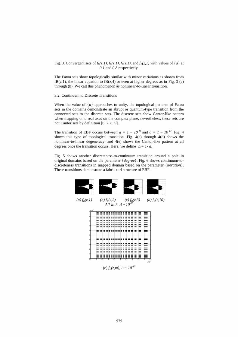
Fig. 3. Convergent sets of fB(z,1), fB(z,1), fB(z,1), and fB(z,1) with values of a at

0.1 and 0.8 respectively.

The Fatou sets show topologically similar with minor variations as shown from

fB(z,1), the linear equation to fB(z,4) or even at higher degrees as in Fig. 3 (e)

through (h). We call this phenomenon as nonlinear-to-linear transition.

3.2. Continuum to Discrete Transitions

When the value of a approaches to unity, the topological patterns of Fatou

sets in the domains demonstrate an abrupt or quantum-type transition from the

connected sets to the discrete sets. The discrete sets show Cantor-like pattern

when mapping onto real axes on the complex plane, nevertheless, these sets are

not Cantor sets by definition [6, 7, 8, 9].

The transition of EBF occurs between a = 1 – 10-16

and a = 1 – 10-17

. Fig. 4

shows this type of topological transition. Fig. 4(a) through 4(d) shows the

nonlinear-to-linear degeneracy, and 4(e) shows the Cantor-like pattern at all

degrees once the transition occurs. Here, we define Δ= 1- a.

Fig. 5 shows another discreteness-to-continuum transition around a pole in

original domains based on the parameter degree. Fig. 6 shows continuum-to-

discreteness transitions in mapped domain based on the parameter iteration.

These transitions demonstrate a fabric tori structure of EBF.

(a) fB(z,1) (b) fB(z,2) (c) fB(z,3) (d) fB(z,10)

All with Δ~ 10-16

(e) fB(z,m),Δ= 10

-17

575

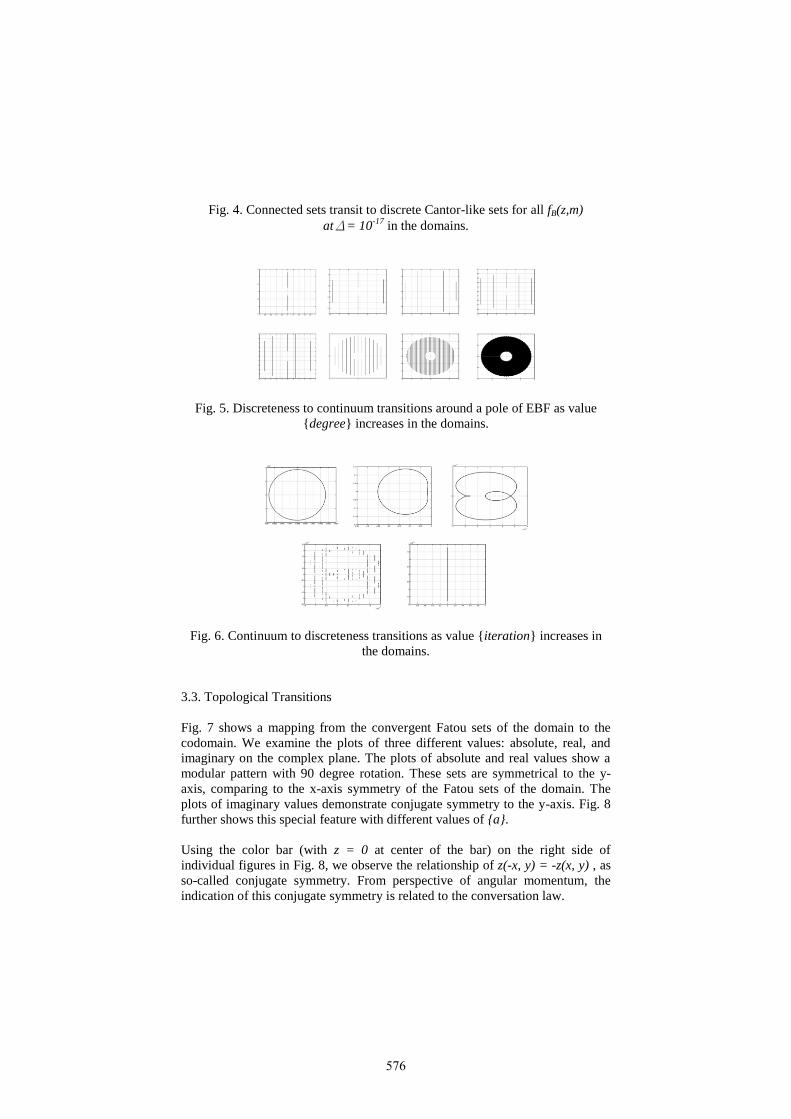
Fig. 4. Connected sets transit to discrete Cantor-like sets for all fB(z,m)

atΔ= 10-17

in the domains.

Fig. 5. Discreteness to continuum transitions around a pole of EBF as value

degree increases in the domains.

Fig. 6. Continuum to discreteness transitions as value iteration increases in

the domains.

3.3. Topological Transitions

Fig. 7 shows a mapping from the convergent Fatou sets of the domain to the

codomain. We examine the plots of three different values: absolute, real, and

imaginary on the complex plane. The plots of absolute and real values show a

modular pattern with 90 degree rotation. These sets are symmetrical to the y-

axis, comparing to the x-axis symmetry of the Fatou sets of the domain. The

plots of imaginary values demonstrate conjugate symmetry to the y-axis. Fig. 8

further shows this special feature with different values of a.

Using the color bar (with z = 0 at center of the bar) on the right side of

individual figures in Fig. 8, we observe the relationship of z(-x, y) = -z(x, y) , as

so-called conjugate symmetry. From perspective of angular momentum, the

indication of this conjugate symmetry is related to the conversation law.

576

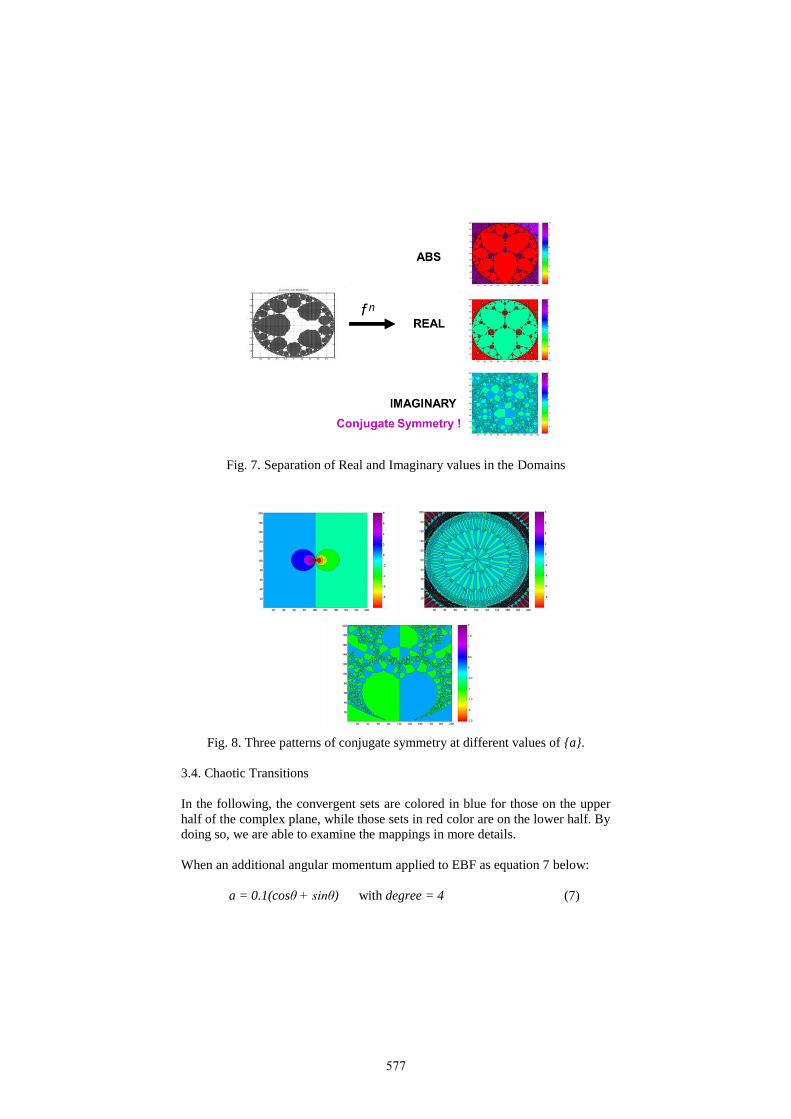
Fig. 7. Separation of Real and Imaginary values in the Domains

Fig. 8. Three patterns of conjugate symmetry at different values of a.

3.4. Chaotic Transitions

In the following, the convergent sets are colored in blue for those on the upper

half of the complex plane, while those sets in red color are on the lower half. By

doing so, we are able to examine the mappings in more details.

When an additional angular momentum applied to EBF as equation 7 below:

a = 0.1(cosθ + sinθ) with degree = 4 (7)

577

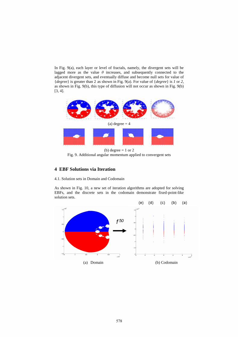
In Fig. 9(a), each layer or level of fractals, namely, the divergent sets will be

lagged more as the value θ increases, and subsequently connected to the

adjacent divergent sets, and eventually diffuse and become null sets for value of

degree is greater than 2 as shown in Fig. 9(a). For value of degree is 1 or 2,

as shown in Fig. 9(b), this type of diffusion will not occur as shown in Fig. 9(b)

[3, 4].

(a) degree = 4

(b) degree = 1 or 2

Fig. 9. Additional angular momentum applied to convergent sets

4 EBF Solutions via Iteration

4.1. Solution sets in Domain and Codomain

As shown in Fig. 10, a new set of iteration algorithms are adopted for solving

EBFs, and the discrete sets in the codomain demonstrate fixed-point-like

solution sets.

(a) Domain (b) Codomain

578

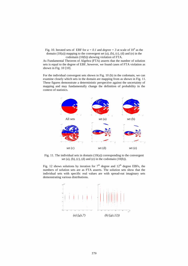
Fig. 10. Iterated sets of EBF for a = 0.1 and degree = 3 at scale of 104 as the

domain (10(a)) mapping to the convergent set (a), (b), (c), (d) and (e) in the

codomain (10(b)) showing violation of FTA.

As Fundamental Theorem of Algebra (FTA) asserts that the number of solution

sets is equal to the degree of EBF, however, we found cases of FTA violation as

shown in Fig. 10 [10].

For the individual convergent sets shown in Fig. 10 (b) in the codomain, we can

examine closely which sets in the domain are mapping from as shown in Fig. 11.

These figures demonstrate a deterministic perspective against the uncertainty of

mapping and may fundamentally change the definition of probability in the

context of statistics.

All sets set (a) set (b)

set (c) set (d) set (e)

Fig. 11. The individual sets in domain (10(a)) corresponding to the convergent

set (a), (b), (c), (d) and (e) in the codomain (10(b)).

Fig. 12 shows solutions by iteration for 7th

degree and 12th

degree EBFs, the

numbers of solution sets are as FTA asserts. The solution sets show that the

individual sets with specific real values are with spread-out imaginary sets

demonstrating various distributions.

(a) fB(z,7) (b) fB(z,12))

579

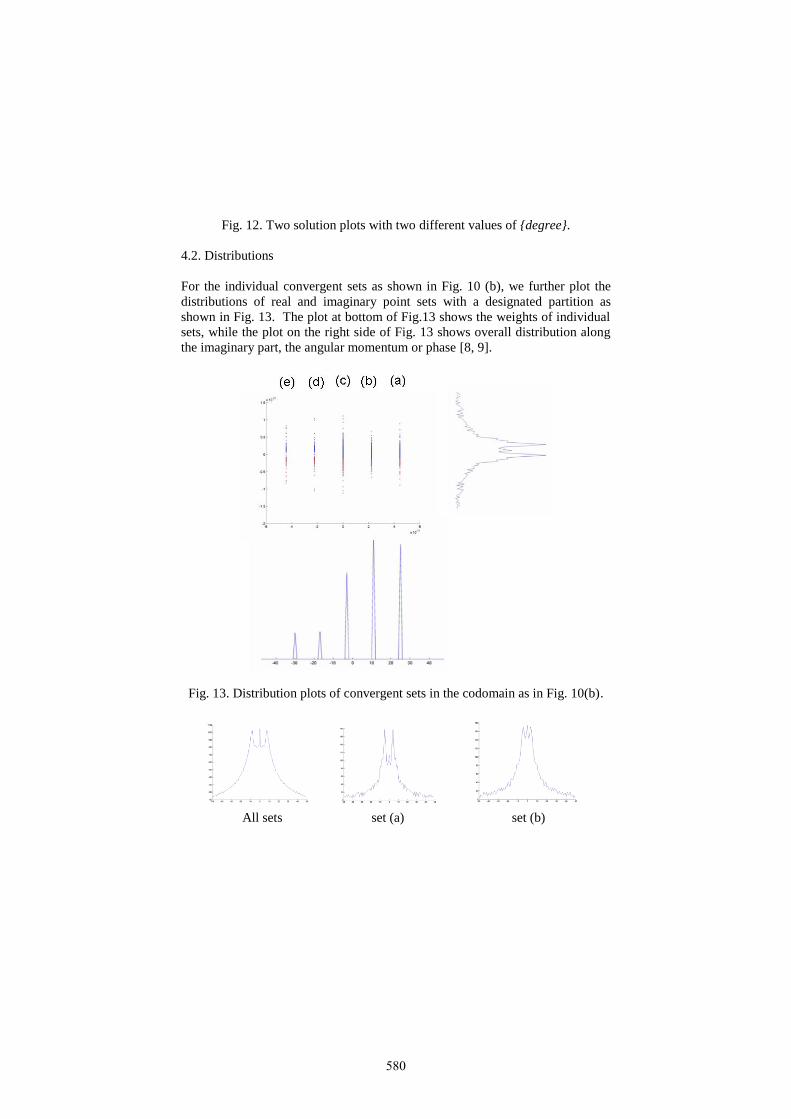
Fig. 12. Two solution plots with two different values of degree.

4.2. Distributions

For the individual convergent sets as shown in Fig. 10 (b), we further plot the

distributions of real and imaginary point sets with a designated partition as

shown in Fig. 13. The plot at bottom of Fig.13 shows the weights of individual

sets, while the plot on the right side of Fig. 13 shows overall distribution along

the imaginary part, the angular momentum or phase [8, 9].

Fig. 13. Distribution plots of convergent sets in the codomain as in Fig. 10(b).

All sets set (a) set (b)

580

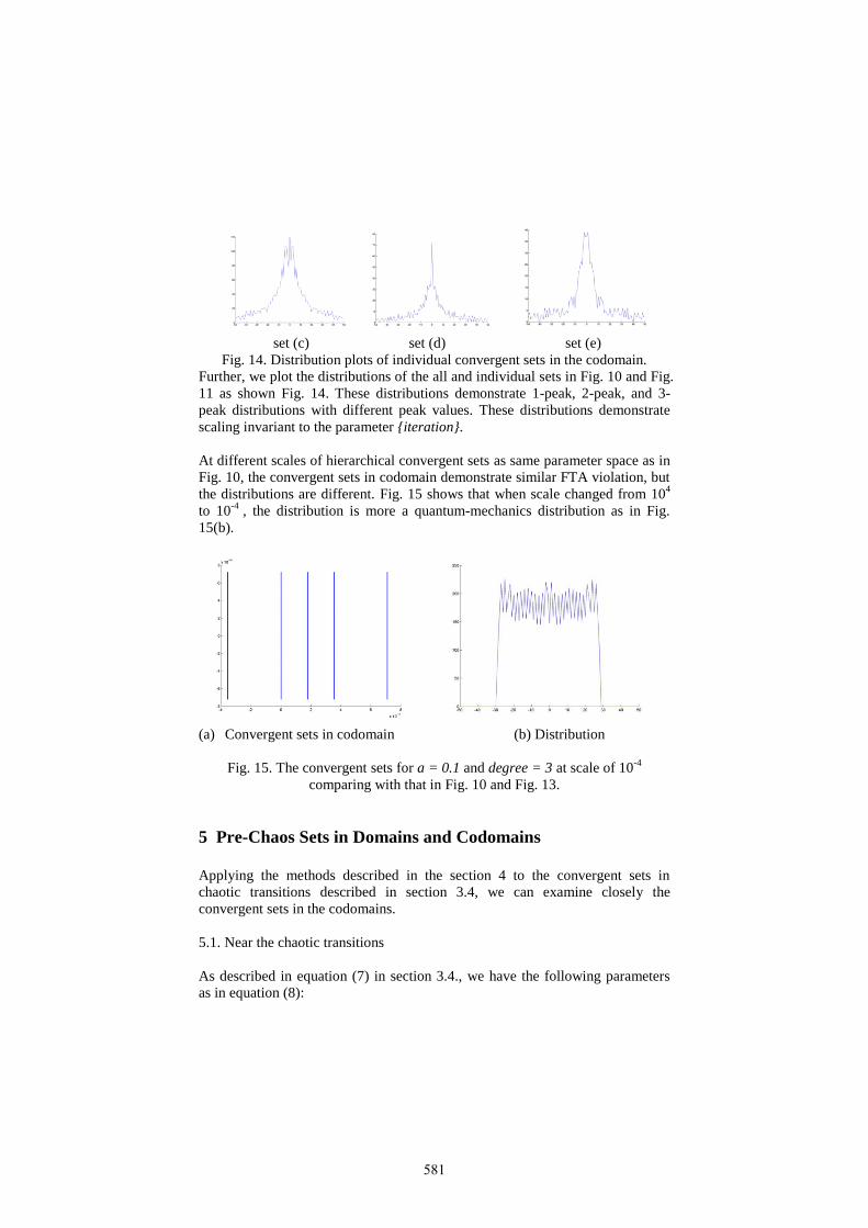
set (c) set (d) set (e)

Fig. 14. Distribution plots of individual convergent sets in the codomain.

Further, we plot the distributions of the all and individual sets in Fig. 10 and Fig.

11 as shown Fig. 14. These distributions demonstrate 1-peak, 2-peak, and 3-

peak distributions with different peak values. These distributions demonstrate

scaling invariant to the parameter iteration.

At different scales of hierarchical convergent sets as same parameter space as in

Fig. 10, the convergent sets in codomain demonstrate similar FTA violation, but

the distributions are different. Fig. 15 shows that when scale changed from 104

to 10-4

, the distribution is more a quantum-mechanics distribution as in Fig.

15(b).

(a) Convergent sets in codomain (b) Distribution

Fig. 15. The convergent sets for a = 0.1 and degree = 3 at scale of 10-4

comparing with that in Fig. 10 and Fig. 13.

5 Pre-Chaos Sets in Domains and Codomains

Applying the methods described in the section 4 to the convergent sets in

chaotic transitions described in section 3.4, we can examine closely the

convergent sets in the codomains.

5.1. Near the chaotic transitions

As described in equation (7) in section 3.4., we have the following parameters

as in equation (8):

581

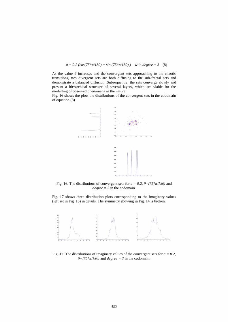
a = 0.2 (cos(75*π/180) + sin (75*π/180) ) with degree = 3 (8)

As the value θ increases and the convergent sets approaching to the chaotic

transitions, two divergent sets are both diffusing to the sub-fractal sets and

demonstrate a balanced diffusion. Subsequently, the sets converge slowly and

present a hierarchical structure of several layers, which are viable for the

modelling of observed phenomena in the nature.

Fig. 16 shows the plots the distributions of the convergent sets in the codomain

of equation (8).

Fig. 16. The distributions of convergent sets for a = 0.2, θ=(75*π/180) and

degree = 3 in the codomain.

Fig. 17 shows three distribution plots corresponding to the imaginary values

(left set in Fig. 16) in details. The symmetry showing in Fig. 14 is broken.

Fig. 17. The distributions of imaginary values of the convergent sets for a = 0.2,

θ=(75*π/180) and degree = 3 in the codomain.

582

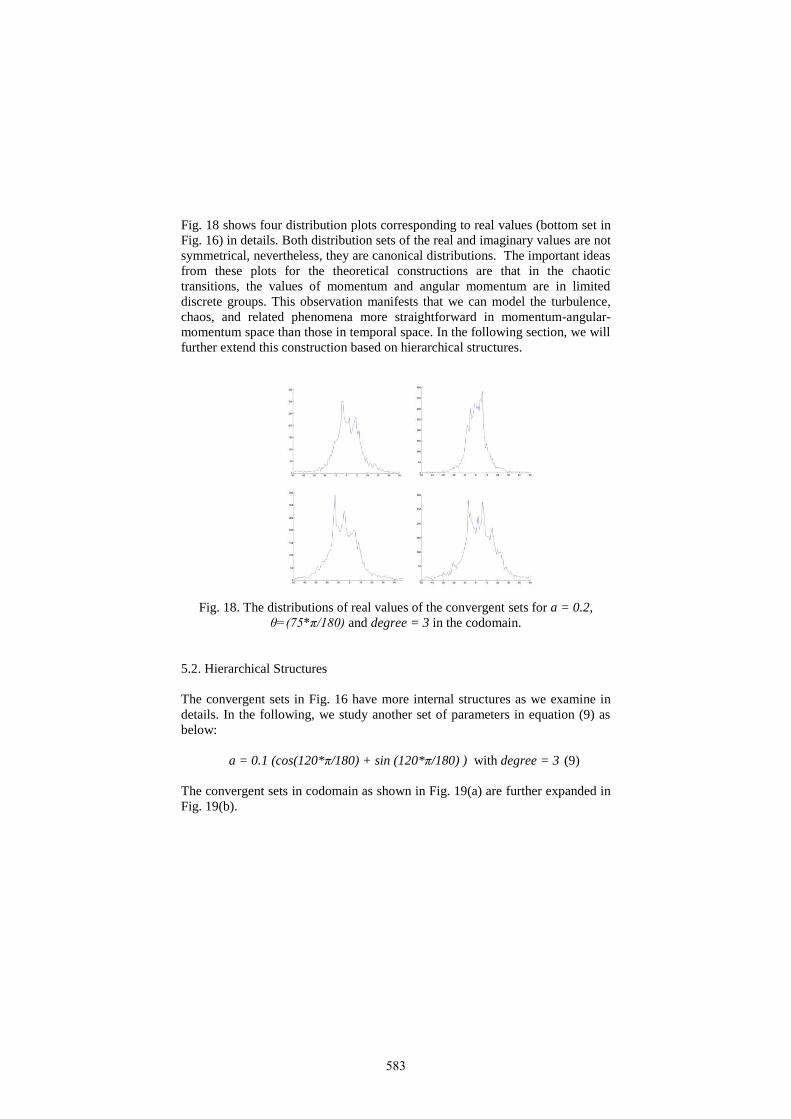
Fig. 18 shows four distribution plots corresponding to real values (bottom set in

Fig. 16) in details. Both distribution sets of the real and imaginary values are not

symmetrical, nevertheless, they are canonical distributions. The important ideas

from these plots for the theoretical constructions are that in the chaotic

transitions, the values of momentum and angular momentum are in limited

discrete groups. This observation manifests that we can model the turbulence,

chaos, and related phenomena more straightforward in momentum-angular-

momentum space than those in temporal space. In the following section, we will

further extend this construction based on hierarchical structures.

Fig. 18. The distributions of real values of the convergent sets for a = 0.2,

θ=(75*π/180) and degree = 3 in the codomain.

5.2. Hierarchical Structures

The convergent sets in Fig. 16 have more internal structures as we examine in

details. In the following, we study another set of parameters in equation (9) as

below:

a = 0.1 (cos(120*π/180) + sin (120*π/180) ) with degree = 3 (9)

The convergent sets in codomain as shown in Fig. 19(a) are further expanded in

Fig. 19(b).

583

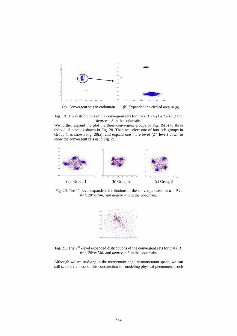
(a) Convergent sets in codomain (b) Expanded the circled area in (a)

Fig. 19. The distributions of the convergent sets for a = 0.1, θ=(120*π/180) and

degree = 3 in the codomain.

We further expand the plot the three convergent groups of Fig. 19(b) to three

individual plots as shown in Fig. 20. Then we select one of four sub-groups in

Group 1 as shown Fig. 20(a), and expand one more level (2nd

level) down to

show the convergent sets as in Fig. 21.

(a) Group 1 (b) Group 2 (c) Group 3

Fig. 20. The 1st

-level expanded distributions of the convergent sets for a = 0.1,

θ=(120*π/180) and degree = 3 in the codomain.

Fig. 21. The 2nd

-level expanded distributions of the convergent sets for a = 0.1,

θ=(120*π/180) and degree = 3 in the codomain.

Although we are studying in the momentum-angular-momentum space, we can

still see the richness of this construction for modeling physical phenomena, such

584

as formation of galaxy cluster and stellar system, statistics related to Boltzmann

Equations and Navier-Stokes equation.

As an example of modeling the formation of our stellar system, we can adopt

the momentum-angular-momentum groups shown in Fig. 21 to the formation of

individual planets from flattening disk of the solar nebular system.

Conclusions

In this paper, we explore the chaotic transition based on the mathematical

construction of the extended Blaschke product (EBP), which can be claimed as

foundation of Nonlinear Relativity. We present the domain-codomain mapping

in the context of dynamical systems, and elaborate the convergent sets of

solution to chaotic transition.

We can summarize our study as follows:

The solution sets of chaotic transitions are discrete, simple, hierarchical,

and slowly convergent in the momentum space comparing with those in

temporal space.

The solution sets of pre-chaos demonstrate discrete distributions and

potentially provide models for formation and structure of galaxy cluster,

Boltzmann Equation, Navier-Stokes equations, among other studies.

The complex functions with conjugate forms produce root counts higher

than that of FTA asserts.

We will further investigate this mathematical construction to the modeling of

chaos in the future.

References

1. W. Blaschke, Eine Erweiterung des Satzes von Vitali, “über Folgen analytischer

Funktionen” Berichte Math.-Phys. Kl., Sächs. Gesell. der Wiss. Leipzig , No. 67, pp.

194–200, 1915.

2. D. C. Ni and C. H. Chin, “Z-1C1C2C3C4 System and Application”, Proceedings of

TIENCS workshop, Singapore, August 1-5, 2006.

3. D. C. Ni and C. H. Chin, Symmetry Broken in Low Dimensional N-body Chaos, Proc.

of Chaos 2009 Conference, Chania, Crete, Greece, pp. 53 (Abstract), June 1-5, 2009.

4. D. C. Ni and C. H. Chin, Symmetry Broken in low dimensional N-Body Chaos,

CHAOTIC SYSTEMS: Theory and Applications (ed. by C. H. Skisdas and I.

Domotikalis), pp. 215-223, 2010

5. D. C. Ni, “Chaotic Behavior Related to Potential Energy and Velocity in N-Body

Systems”, Proceedings of 8th AIMS International Conference on Dynamical Systems,

Differential Equations and Applications, May 25-28, 2010, Dresden, Germany, pp.

328.

585

6. D. C. Ni and C. H. Chin, “Classification on Herman Rings of Extended Blaschke

Equations”, Differential Equations and Control processes, Issue No. 2, Article 1,

2010.

(http://www.neva.ru/journal/j/EN/numbers/2010.2/issue.html).

7. D. C. Ni, “Numerical Studies of Lorentz Transformation”, Proceeding of 7th

EASIAM, Kitakyushu, Japan, June 27-29, 2011, pp. 113-114.

8. D. C. Ni, “Statistics constructed from N-body systems”, Proceeding of World

Congress, Statistics and Probability, Istanbul, Turkey, July 9-14, 2012, pp. 171.

9. D. C. Ni, “Phase Transition Models based on A N-Body Complex Statistics”,

Proceedings of the World Congress on Engineering 2013 (WCE 2013), Vol I, pp.

319-323, , July 3 - 5, 2013, London, U.K.

10. D.C. Ni, “A Counter Example of Fundamental Theorem of Algebra: Extended

Blaschke Mapping”, Proceedings of ICM 2014, August 13-August 21, Seoul, Korea,

2014.

586

From chaotic motion to Brownian motion.

A survey and some connected problems

Gabriel V. Orman and Irinel Radomir

Department of Mathematics and Computer Science ”Transilvania” University ofBrasov, 500091 Brasov, Romania(E-mail: ogabriel@unitbv.ro)

Abstract. In this paper we shall refer to the passing from chaotic motion toBrownian motion. To this end a review of some aspects concerning the Markoviannature of the Brownian path is presented. We discuss about some interesting resultsregarding to the 3-dimensional Brownian motion in connection with the Markovprocess in a generalized sense and the k-dimensional Brownian motion in connectionwith the Dirichlet problem. Then, we shall refer to some special connected studies.

Keywords: stochastic calculus, Markov processes, Markov property, Brownianmotion, convergence.

1 Introduction

Let us imagine a chaotic motion of a particle of colloidal size immersed in a fluid.Such a chaotic motion of a particle is called, usually, Brownian motion and theparticle which performs such a motion is referred to as a Brownian particle. Sucha chaotic perpetual motion of a Brownian particle is the result of the collisions ofparticle with the molecules of the fluid in which there is.

But this particle is much bigger and also heavier than the molecules of thefluid which it collide, and then each collision has a negligible effect, while thesuperposition of many small interactions will produce an observable effect.

On the other hand, for a Brownian particle such molecular collisions appear ina very rapid succession, their number being enormous. For a so high frequency,evidently, the small changes in the particle’s path, caused by each single impact,are too fine to be observable. For this reason the exact path of the particle can bedescribed only by statistical methods.

Used especially in Physics, Brownian motion is of ever increasing importancenot only in Probability theory but also in classical Analysis. Its fascinating proper-ties and its far-reaching extension of the simplest normal limit theorems to func-tional limit distributions acted, and continue to act, as a catalyst in random ana-lysis. As some authors remarks too, the Brownian motion reflects a perfection thatseems closer to a law of nature than to a human invention.

Brownian motion was frequently explained as due to the fact that particles werealive.

We remind that Poincare thought that it contradicted the second law of Ther-modynamics._________________

8th CHAOS Conference Proceedings, 26-29 May 2015, Henri Poincaré Institute, Paris France

© 2015 ISAST

587

Today we know that this motion is due to the bombardament of the particlesby the molecules of the medium. In a liquid, under normal conditions, the orderof magnitude of the number of these impacts is of 1020 per second. It is only in1905 that kinetic molecular theory led Einstein to the first mathematical modelof Brownian motion. He began by deriving its possible existence and then onlylearned that it had been observed.

A completely different origin of mathematical Brownian motion is a game the-oretic model for fluctuations of stock prices due to L. Bachelier from 1900.

In the sequel we shell refer shortly to his vision. At the same time we shalldiscuss some aspects regarding the Markovian nature of the Brownian path, the 3-dimensional Brownian motion in connection with a Markov process in a generalizedsense and the extension to the k-dimensional Brownian motion. Finally, we shallrefer shortly to some special connected studies.

2 The Markovian nature of the Brownian path

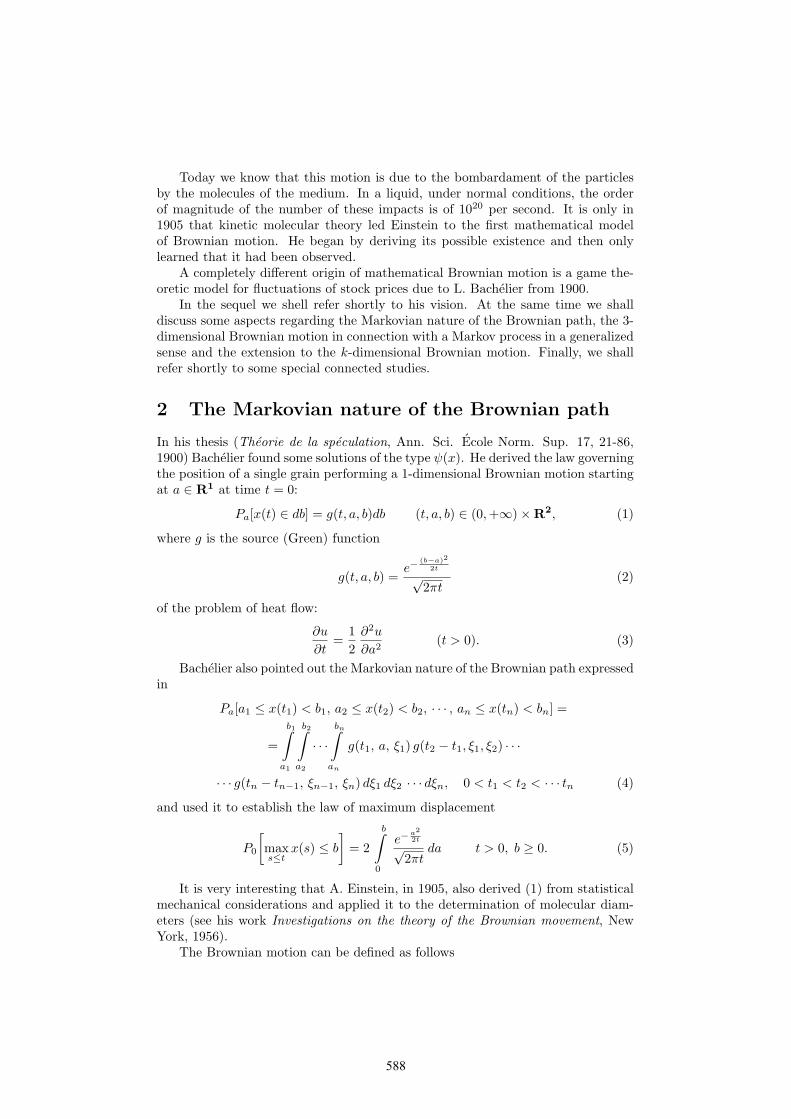
In his thesis (Theorie de la speculation, Ann. Sci. Ecole Norm. Sup. 17, 21-86,1900) Bachelier found some solutions of the type ψ(x). He derived the law governingthe position of a single grain performing a 1-dimensional Brownian motion startingat a ∈ R1 at time t = 0:

Pa[x(t) ∈ db] = g(t, a, b)db (t, a, b) ∈ (0,+∞)×R2, (1)

where g is the source (Green) function

g(t, a, b) =e−

(b−a)2

2t

√2πt

(2)

of the problem of heat flow:

∂u

∂t=

12∂2u

∂a2(t > 0). (3)

Bachelier also pointed out the Markovian nature of the Brownian path expressedin

Pa[a1 ≤ x(t1) < b1, a2 ≤ x(t2) < b2, · · · , an ≤ x(tn) < bn] =

=

b1∫a1

b2∫a2

· · ·bn∫an

g(t1, a, ξ1) g(t2 − t1, ξ1, ξ2) · · ·

· · · g(tn − tn−1, ξn−1, ξn) dξ1 dξ2 · · · dξn, 0 < t1 < t2 < · · · tn (4)

and used it to establish the law of maximum displacement

P0

[maxs≤t

x(s) ≤ b]

= 2

b∫0

e−a22t

√2πt

da t > 0, b ≥ 0. (5)

It is very interesting that A. Einstein, in 1905, also derived (1) from statisticalmechanical considerations and applied it to the determination of molecular diam-eters (see his work Investigations on the theory of the Brownian movement, NewYork, 1956).

The Brownian motion can be defined as follows

588

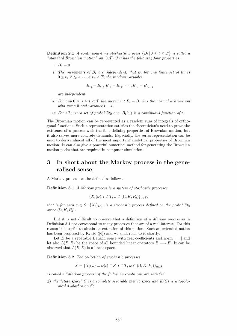
Definition 2.1 A continuous-time stochastic process Bt | 0 ≤ t ≤ T is called a”standard Brownian motion” on [0, T ) if it has the following four properties:

i B0 = 0.

ii The increments of Bt are independent; that is, for any finite set of times0 ≤ t1 < t2 < · · · < tn < T, the random variables

Bt2 −Bt1 , Bt3 −Bt2 , · · · , Btn −Btn−1

are independent.

iii For any 0 ≤ s ≤ t < T the increment Bt − Bs has the normal distributionwith mean 0 and variance t− s.

iv For all ω in a set of probability one, Bt(ω) is a continuous function of t.

The Brownian motion can be represented as a random sum of integrals of ortho-gonal functions. Such a representation satisfies the theoretician’s need to prove theexistence of a process with the four defining properties of Brownian motion, butit also serves more concrete demands. Especially, the series representation can beused to derive almost all of the most important analytical properties of Brownianmotion. It can also give a powerful numerical method for generating the Brownianmotion paths that are required in computer simulation.

3 In short about the Markov process in the gene-ralized sense

A Markov process can be defined as follows:

Definition 3.1 A Markov process is a system of stochastic processes

Xt(ω), t ∈ T, ω ∈ (Ω,K, Pa)a∈S ,

that is for each a ∈ S, Xtt∈S is a stochastic process defined on the probabilityspace (Ω,K, Pa).

But it is not difficult to observe that a definition of a Markov process as inDefinition 3.1 not correspond to many processes that are of a real interest. For thisreason it is useful to obtain an extension of this notion. Such an extended notionhas been proposed by K. Ito ([6]) and we shall refer to it shortly.

Let E be a separable Banach space with real coefficients and norm || · || andlet also L(E,E) be the space of all bounded linear operators E −→ E. It can beobserved that L(E,E) is a linear space.

Definition 3.2 The collection of stochastic processes

X = Xt(ω) ≡ ω(t) ∈ S, t ∈ T, ω ∈ (Ω,K, Pa)a∈S

is called a ”Markov process” if the following conditions are satisfied:

1) the ”state space” S is a complete separable metric space and K(S) is a topolo-gical σ-algebra on S;

589

2) the ”time internal” T = [0,∞);

3) the ”space of paths” Ω is the space of all right continuous functions T −→ Sand K is the σ-algebra K[Xt : t ∈ T ] on Ω;

4) the probability law of the path starting at a, Pa(H), is a probability measure on(Ω,K) for every a ∈ S which satisfy the following conditions:

4a) Pa(H) is K(S)-measurable in a for every H ∈ K;

4b) Pa(X0 = a) = 1;

4c) Pa(Xt1 ∈ E1, · · · , Xtn ∈ En) =∫. . .

∫ai∈Ei

Pa(Xt1 ∈ da1)Pa1(Xt2−t1 ∈ da2) . . .

. . . Pan−1(Xtn−tn−1 ∈ dan) for 0 < t1 < t2 < . . . < tn.

According to Definition 3.2, X will be referred as a Markov process in thegeneralized sense.

Now let X be a Markov process in a generalized sense and let us denote byB(S) the space of all bounded real K(S)-measurable functions. Also let us considera function f ∈ B(S).

It is supposed that

Ea

( ∞∫0

|f(Xt)|dt)

(6)

is bounded in a. Therefore

Uf(a) = Ea

( ∞∫0

f(Xt)dt)

(7)

is well-defined and is a bounded K(S)-measurable function of a ∈ S.The Uf is called the potential of f with respect to X. Having in view that

Uf = limα↓0Rαf , it is reasonable to write R0 instead of U . Based on this fact,Rαf will be called the potential of order α of f .

Remark 3.1 It is useful to retain that Rαf ∈ B(S) for α > 0; and generallyf ∈ B(S) while R0f(= Uf) ∈ B(S) under the condition (6).

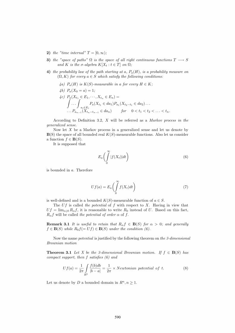
Now the name potential is justified by the following theorem on the 3-dimensionalBrownian motion

Theorem 3.1 Let X be the 3-dimensional Brownian motion. If f ∈ B(S) hascompact support, then f satisfies (6) and

Uf(a) =1

2π

∫R3

f(b)db|b− a|

=1

2π×Newtonian potential of t. (8)

Let us denote by D a bounded domain in Rn, n ≥ 1.

590

Definition 3.3 A function g is called ”harmonic” in D if g is C∞ in D and if∆g = 0 (where C∞ is the class of functions differentiable infinitely many times).

Now let f be a continuous function defined on the boundary ∂D and let usdenote by X a k-dimensional Brownian motion defined as follows

Definition 3.4 The k-dimensional Brownian motion is defined on S = Rk by theequality

pt(a, db) = (2πt)−k2 e−

|b−a|22t db = Nt(b− a)db,

where |b− a| is the norm of b− a in Rk.

Given a k-dimensional Brownian motion X, if there exists a solution g for theDirichlet problem (D, f)1, then

g(a) = Ea(f(Xλ)), (9)

where λ ≡ λD = exit time from D (that is to say λD = inft > 0 : Xt 6∈ D, thehitting time of DC).

In this context an interesting result is given in the following theorem

Theorem 3.2 If D is a bounded domain and g is a solution of the Dirichlet problem(D, f), then

g(a) = Ea(f(Xλ))

where a ∈ D and λ = λD.

On the other hand, the Dirichlet problem (D, f) has a solution if ∂D is smoothas it is prooved in the following theorem

Theorem 3.3 If ∂D is smooth, then

g(a) = Ea(f(Xλ)),

where λ = λD = exit time fromD, is the solution of the Dirichlet problem (D, f).

Note 3.1 The expression ”∂D is smooth” means that ∂D has a unic tangent planeat each point x of ∂D and the outward unit normal of the tangent plane at x movescontinously with x.

4 A general survey of some special connectedstudies

Bachelier was unable to obtain a clear picture of the Brownian motion and hisideas were unappreciated at that time. This because a precise definition of theBrownian motion involves a measure on the path space, and it was not until 1909when E. Borel published his classical memoir on Bernoulli trials (Les probabilites

1The Diriclet problem (D, f) is to find a continuous function g = gD,f on the closure

D ≡ D ∪ ∂D such that g is harmonic in D and g = f g ∂D.

591

denombrables et leurs applications arithmetique Rend. Circ. Mat. Palermo 27,1909, 247-271.

As soon as the ideas of Borel, Lebesgue and Daniell appeared, it was possible toput the Brownian motion on a firm mathematical foundation and this was achivedby N. Wiener in 1923 (Differential space, J. Math. Phis. 2,1923, 131-174).

Many researchers were fascinated by the great beauty of the theory of Brownianmotion and many results have been obtained in the last decades. As for example,among other things, in Diffusion processes and their sample paths by K. Ito andH.P. McKean, Jr., in Theory and applications of stochastic differential equations byZ. Schuss, or in Stochastic approximation by M.T. Wasan as in Stochastic calculusand its applications to some problems in finance by J.M. Steele. In this context onecan consider also our book Aspects of convergence and approximation in randomsystems analysis.

As we have already emphasized a rigorous definition and study of (mathema-tical) Brownian motion requires measure theory.

Consider the space of continuous path w : t ∈ [0,+∞)→ R1 with coordinatesx(t) = w(t) and let β be the smallest Borel algebra of subsets B of this path spacewhich includes all the simple events

B = (w : a ≤ x(t) < b), (t ≥ 0, a < b).

Wiener established the existence of non-negative Borel measures Pa(B), (a ∈ R1, B ∈β) for which (4) holds. Among other things, this result attaches a precise meaningto Bachelier’s statement that the Brownian path is continuous.

Paul Levy (Sur certain processus stochastiques homogenes, Compositio Math.7, 1939, pp. 283-339) found another construction of the Brownian motionand also gave a profound description of the fine structure of the individualBrownian path2.

Levy’s results with several complements due to D.B. Ray (Sojourn timesof a diffusion process, IJM 7, 1963, 615-630) and K. Ito & H.P. McKean Jr.(Diffusion processes and their Sample Path, Springer-Verlag Berlin heidel-berg, 1956) are of a special attention to the standard Brownian local time(la measure du voisinage of P. Levy):

τ(t, a) = limb↓ameasure(s : a ≤ x(s) < b, s ≤ t)

2(b− a). (10)

Given a Sturm-Liouville operator

D(c2/2)D2 + c1D, c2 > 0

on the line, the source (Green) function p = p(t, a, b) of the problem

∂u

∂t= Du, t > 0 (11)

share with the Gauss kernel g of (2) the properties:(a) 0 ≤ p

2P. Levy, Processus stochastiques et mouvement brownien, Paris, 1948

592

(b)∫R1 p(t, a, b)db = 1

(c) p(t, a, b) =∫R1 p(t− s, a, c)p(s, c, b)dc, t > s > 0.

Soon after the publication of Wiener’s monograph (Generalized harmonicana-lysis, Acta Math. 5, 1930, 117-258), the associated stochastic motions(diffusions) analogous to the Brownian motion (D = D2/2) made their de-but. At a later date (1946) K. Ito (On a stochastic integral equation, Proc.Japan acad. 22, 1946, 32-35) proved that if

|c1(b)− c1(a)|+ |√c2(b)−

√c2(a)| < constant× |b− a|, (12)

then the motion associated with

D = (c2/2)D2 + c1D

is identical in law to the ”continuous” solution of

a(t) = a(0) +∫ t

0c1(a)ds+

∫ t

0

√c2(a)db (13)

where b is a standard Brownian motion.W. Feller took to lead in the next development. Given a Markovian

motion with sample paths w : t → x(t) and probabilities Pa(B) on a linearinterval Q, the operators

Ht : f →∫Pa[x(t) ∈ db]f(b) (14)

constitute a semi-group :

Ht = Ht−sHs, t ≥ s (15)

and as E. Hille (Represenation of one-parameter semi-groups of linear tans-formations, PNAS 28, 1942, 175-178) and K. Yosida (On the differentiabilityand the representation of one-parameter semi-group of linear operators, J.Math. Soc. Japan 1, 1948, 15-21) proved,

Ht = etD, t > 0 (16)

with a suitable interpretation of the exponential, where D is the so-calledgenerator.

We mention again the name of D. Ray to emphasize that he proved(Stationary Markov processes with continuos path, TAMS, 82, 1956, pp.452-493) that if the motion is strict Markov (i.e. if it starts afresh at certainstochastic (Markov) times including that passage times ma = min(t : x(t) =a), etc.), then the so-called generator D is local if and only if the motionhas continuous sample paths, substantiating a conjecture of W. Feller.

593

Then by combining this with some other Feller’s papers as

•W. Feller, The paraboloc differential equations and the associated semi-groups of tansformaions, AM 55, 1952, 468-519;• W. Feller, The general diffusion operator and positivity preserving

semi-groups in one dimension, AM 60, 1954, 417-436;•W. Feller, On second order differential operators, AM 61, 1955, 90-105;• W. Feller, Generalized second order differential operators and their

lateral conditions, IJM 1, 1957, 456-504,

it is implied that the generator of a strict Markovian motion with continuouspaths (diffusion) can be expressed as a differential operator

(Du)(a) = limb↓a

u+(b)− u+(a)m(a, b)

, (17)

where m is a non-negative Borel measure positive on open intervals and,with a change of scale

u+(a) = limb↓a

(b− a)−1 [u(b)− u(a)],

except of certain singular points where D degenerates to a differential oper-ator of degreee ≤ 1.

Finally we remark that E.B. Dynkin (Continous one-dimensional Markovprocesses, Dokl. Akad. Nauk SSSR, 105, 1955, 405-408) also arrived at theidea of a stict Markov process. He derived an elegant formula for D andused it to make a simple (proba-bilistic) proof of Feller’s expression for D.

At the same time we consider that the papers of R. Blumenthal - Anextended Markov property, TAMS 85, 1957, 52-72, and G. Hunt - Sometheorems concerning Brownian motion, TAMS 81, 1956, 294-319, as well asthe monographs of E.B. Dynkin - Principles of the theory of Markov randomprocesses, Moskow-Leningrad, 1959; and Markov processes, Moskow, 1963,must also to be mentioned in such a connection.q

Remark 4.1 Many other details regarding to the topics just discussed, proofsand some related problems can be found in [6], [5], [1], [4], [21], [10], [22],[9], [15], [13].

References

[1] Bharucha-Reid, A.T. Elements of the Theory of Markov Processes andTheir Applications. Dover Publications, Inc., Mineola, New York, 1997.

[2] Gihman, I.I. and Skorohod, A.V. Stochastic Differential Equations.Spriger-Verlag, Berlin, 1972.

594

[3] Gnedenko, B.V. The Theory of Probability. Mir Publisher, Moskow,1976.

[4] K. Ito. Selected Papers. Springer, 1987.

[5] K. Ito and H.P. McKean Jr. Diffusion Processes and their Sample Paths.Springer-Verlag, Berlin Heidelberg, 1996.

[6] Ito, K. Stochastic Processes. Edited by Ole E. Barndorff-Nielsen, Ken-iti Sato. Springer, 2004.

[7] Kushner, H.J. and Yin, G.G. Stochastic Approximation Algorithms andApplications. Springer-Verlag New York, Inc., 1997.

[8] Øksendal, B. Stochastic Differential Equations: An Introduction withApplications. Sixth Edition. Springer-Verlag, 2003.

[9] Øksendal, B. and Sulem, A. Applied Stochastic Control of Jump Dif-fusions. Springer, 2007.

[10] P. Olofsson and M. Andersson. Probability, Statistics and StochasticProcesses, 2nd Edition. John Wiley & Sons, Inc., Publication, 2012.

[11] Orman, G.V. Lectures on Stochastic Approximation Methods and Re-lated Topics. ”Gerhard Mercator” University, Duisburg, Germany,2001.

[12] Orman, G.V. Handbook of Limit Theorems and Stochastic Approxi-mation. Transilvania University Press, Brasov, 2003.

[13] G.V. Orman. On Markov Processes: A Survey of the Transition Prob-abilities and Markov Property. In C. H. Skiadas and I. Dimotikalis,editors, Chaotic Systems: Theory and Applications, World ScientificPublishing Co Pte Ltd., 224-232, 2010.

[14] Orman, G.V. On a Problem of Approximation of Markov Chains by aSolution of a Stochastic Differential Equation. In: Christos H. Skiadas,Ioannis Dimotikalis and Charilaos Skiadas (Eds.) Chaos Theory: Mod-eling, Simulation and Applications. World Scientific Publishing Co PteLtd., 2011, 30-40.

[15] Orman, G.V. and Radomir, I. New Aspects in Approximation of aMarkov Chain by a Solution of a Stochastic Differential Equation.Chaotic Modeling and Simulation (CMSIM) International Journal,2012, 711-718.

[16] Orman, G.V. Aspects of convergence and approximation in randomsystems analysis. LAP Lambert Academic Publishing, 2012.

595

[17] Orman, G.V. and Radomir, I. On Stochastic Calculus and DiffusionApproximation to Markov Processes. In: Chaos and Complex Systems,Eds. S.G. Stavrinides, S. Banerjee, S.H. Caglar, M. Ozer, Springer-Verlag Berlin Heidelberg 2013, 239-244.

[18] Orman, G.V. Basic Probability Theory, Convergence, Stochastic Pro-cesses and Applications (to appear).

[19] Qi-Ming He. Fundamentals of Matrix-Analytic Methods. Springer NewYork, 2014.

[20] Steele, J. M. Stochastic Calculus and Financial Applications. Springer-Verlag New York, Inc., 2001.

[21] Stroock, D. W. Markov Processes from K. Ito Perspective. PrincetonUniv. Press, Princeton, 2003.

[22] Schuss, Z. Theory and Application of Stochastic Differential Equations.John Wiley & Sons, New York, 1980.

[23] Wasan, M.T. Stochastic Approximation. Cambridge University Press,1969.

596

_________________

8th

CHAOS Conference Proceedings, 26-29 May 2015, Henri Poincaré Institute, Paris France

© 2015 ISAST

An Analysis Study on Role of Chaos in Symmetric

Encryption Algorithm

Fatih Özkaynak1, Ahmet Bedri Özer2

1 Fırat University, Department of Software Engineering, 23119 Elazig, Turkey

(E-mail: ozkaynak_fatih@hotmail.com) 2

Fırat University, Department of Computer Engineering, 23119 Elazig, Turkey

(E-mail: bedriozer@firat.edu.tr)

Abstract. In this study, we examine randomness properties of chaos based cryptographic designs. The analysis studies show that chaotic outputs which are used as a source of randomness, successfully pass the standard statistical tests, but their cryptographic randomness properties are worse than any standard random function. With these results, suitability of digital chaos in new cryptologic designs should be re-evaluated by the

chaotic cryptology literature. Keywords: Chaos; Cryptography; Cryptographically randomness; Effect of computation precision; Digital chaos.

1 Introduction

Basic goal of modern cryptography is ensuring security of communication

across an insecure medium such as Internet. In order to achieve this goal,

modern cryptography supplies a protocol. Briefly, the modern cryptography is

about constructing and analyzing protocols which overcome the influence of

adversaries [1-4]. A protocol is a collection of programs. These programs tell each party how to behave. A protocol can be probabilistic. This means that it

can make random choices. Therefore, pseudo random functions are central tools

in the design of protocols. A pseudo random function is a family of functions

with the property that the input-output behavior of a random instance of the

family is “computationally indistinguishable” from that of a random function [1,

2].

Chaos theory has been developed to model complex behavior using quite

simple mathematical models. Chaotic systems are the highly unpredictable and

random-looking signals [5]. In theory, there is a relationship between chaos and

cryptography. The main characteristics of chaotic dynamics (dependency on the

initial conditions and control parameters, ergodicity, mixing) are connected to the requirements of cryptography (confusion and diffusion of information) [6,

7].

Although there are number of chaos based cryptologic system proposals in

the literature, it is curious that the subject is quite far from mainstream

cryptology literature [8, 9]. This is largely because of the misinterpretation of

597

the relationship between chaos and cryptology sciences. Chief aim of the

cryptology science is to design and analyze the protocols to provide secure

communication. Theoretically even if it is possible to use the chaotic systems

during protocol design stage, [10-19] when practical applications considered

there are several deficient problems [20-27, 37]. This study analyses the effects of chaotic system behaviors over

cryptography systems depending on computational precision, when definite

chaotic systems are used as pseudo random processes during cryptologic

protocol design. As the result of analyses it is revealed that, although chaotic

outputs successfully pass the standard statistical tests but, their randomness

properties are worse than any standard random function. With this result, it is

shown that neither digital chaos is suitable for cryptologic designs nor the

statistical test packages are cryptographically adequate.

The outline of the study is as follows. In the next section, we examine basic

problems of chaos based cryptography. In section 3, we show that effect of

computational precision in chaotic systems. In the section 4, we present the

summary of the random mapping statistics. In Section 5, we demonstrate performance comparisons. Finally, we give concluding remarks.

2 Problems of Chaos Based Cryptography In the cryptography, there are two development paradigms, namely

cryptanalysis-driven design and proof-driven design [1-3]. Chaos based

cryptography studies have been used cryptanalysis-driven design paradigm. This paradigm has worked something like this.

1. A cryptographic goal is recognized.

2. A solution is offered.

3. One searches for an attack on the proposed solution.

4. When one is found, if it is deemed damaging or indicative of a

potential weakness, you go back to Step 2 and try to come up with a

better solution. The process then continues.

There are some difficulties with the approach of cryptanalysis-drive design. The obvious problem is that one never knows if things are right, nor when one is

finished! The process should iterate until one feels “confident” that the solution

is adequate. But one has to accept that design errors might come to light at any

time. Despite that problem, cryptanalysis-drive design process is still

employable. However, the main problem of chaos based cryptographic designs

is the usage of very simple statistical tests for cryptanalysis studies. For

example, NPCR (number of pixels change rate), UACI (unified average

changing intensity) and histogram analysis have been used for differential and

linear cryptanalysis of almost all chaos based image encryption algorithms.

In addition to the problems arising from the analysis, the fact that the chaotic

systems are realized on digital computers is another issue to be evaluated. While cryptologic designs use a finite set of integers as the workspace, chaotic systems

use a set of real numbers [20]. As a result, simulations of chaotic systems on

digital computers suffer from truncation and round-off errors. In consequence,

598

random behavior expected from chaos is replaced with periodical behavior

which does not meet the confusion and diffusion requirements of the cryptologic

designs. This effect is shown in detail in next section.

3 Effects of Computational Precision in Chaotic Systems Data representation is one of the most important theoretical problems for the

computers which are designed to process, control and store of data. Data types

like integers, real numbers or strings can be infinite by nature. However, since

computers only have finite computational capacity, numerical errors will arise

depending on computational precision. These numerical errors cause different

data values to be perceived as representing the same value. Pigeonhole

principle which is one of the most powerful tools in computer science can be applied to show this problem theoretically. If there are more pigeons than holes

they occupy, then at least two pigeons must be in the same hole.

Theorem: (Pigeonhole Principle). If , then for every total

function , there exist two different elements of that are

mapped by to the same element of .

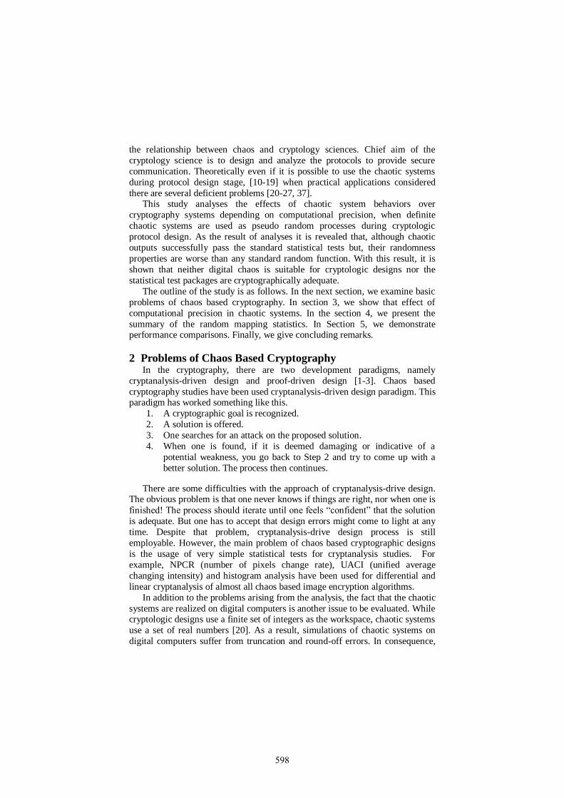
In the interval [0, 1], there are infinitely real numbers. Let’s consider

representing these numbers with 4 bits computational precision. In such case,

the [0, 1] interval will be divided into 24-1=15 different intervals. The upper and

lower limits of those 15 intervals will be as shown in Fig 1. This implies that all

real numbers falling into same interval will be represented with a single value,

for instance all real numbers between 0.0625 and 0.1250 will be represented as

0,0625, producing numerical errors in all computations. This type of numerical

errors will affect the pseudorandom behavior of the chaotic system. To

illustrate, a logistic map implemented on a computer with 4 bits computational

precision and the resulting trajectories are shown in Fig. 2. Although there are

24-1=15 different intervals and theoretically it is expected to obtain 15 different trajectories, only 2 different trajectories are obtained.

Fig. 1. Computation intervals for 4 bits computational precision

4 Properties of Random Mapping

Let be a function, , where denote the finite domain of size

and let denote the collection of all functions where every function is equally

likely to be chosen. So the sample space consists of random mappings, in

other words, the probability that a particular function from is chosen is

. Starting from a point and iteratively applying , the following

sequence is obtained;

(1)

599

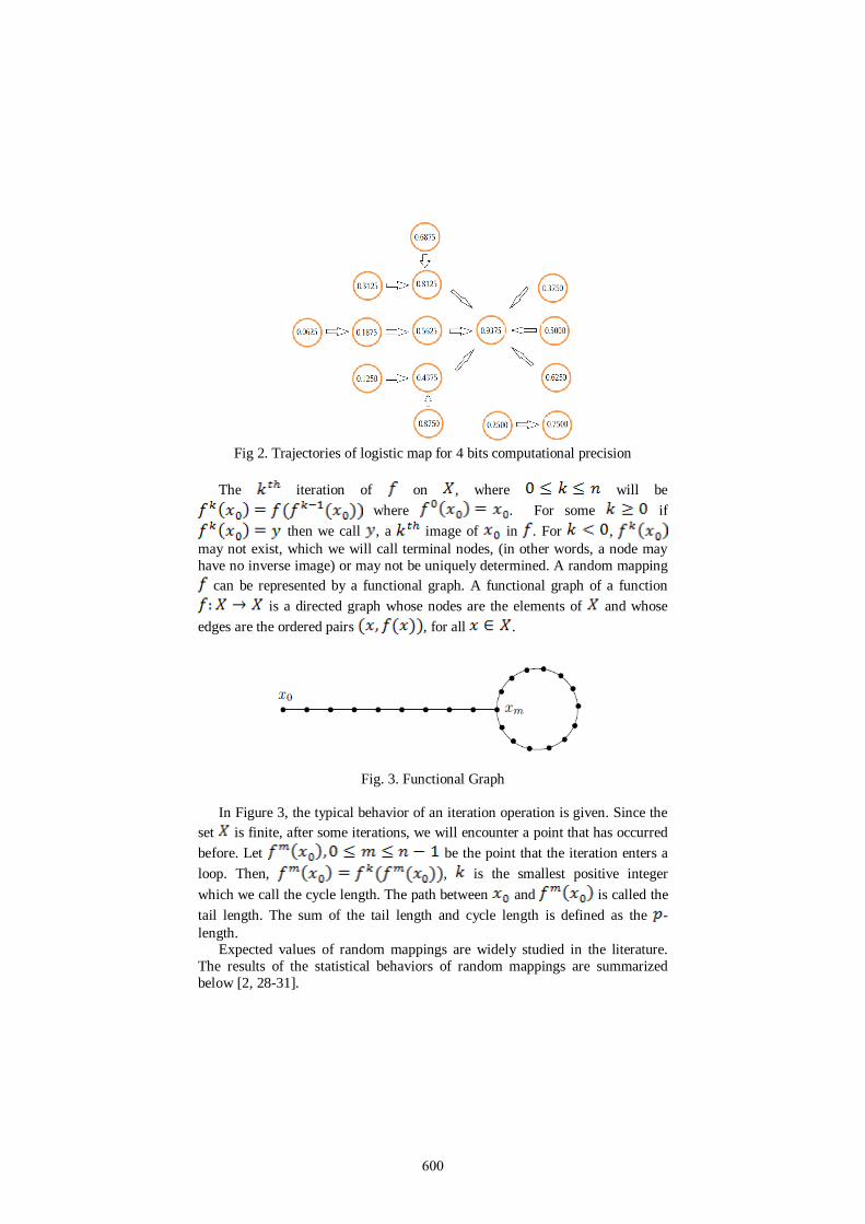
Fig 2. Trajectories of logistic map for 4 bits computational precision

The iteration of on , where will be

where . For some if

then we call , a image of in . For ,

may not exist, which we will call terminal nodes, (in other words, a node may

have no inverse image) or may not be uniquely determined. A random mapping

can be represented by a functional graph. A functional graph of a function

is a directed graph whose nodes are the elements of and whose

edges are the ordered pairs , for all .

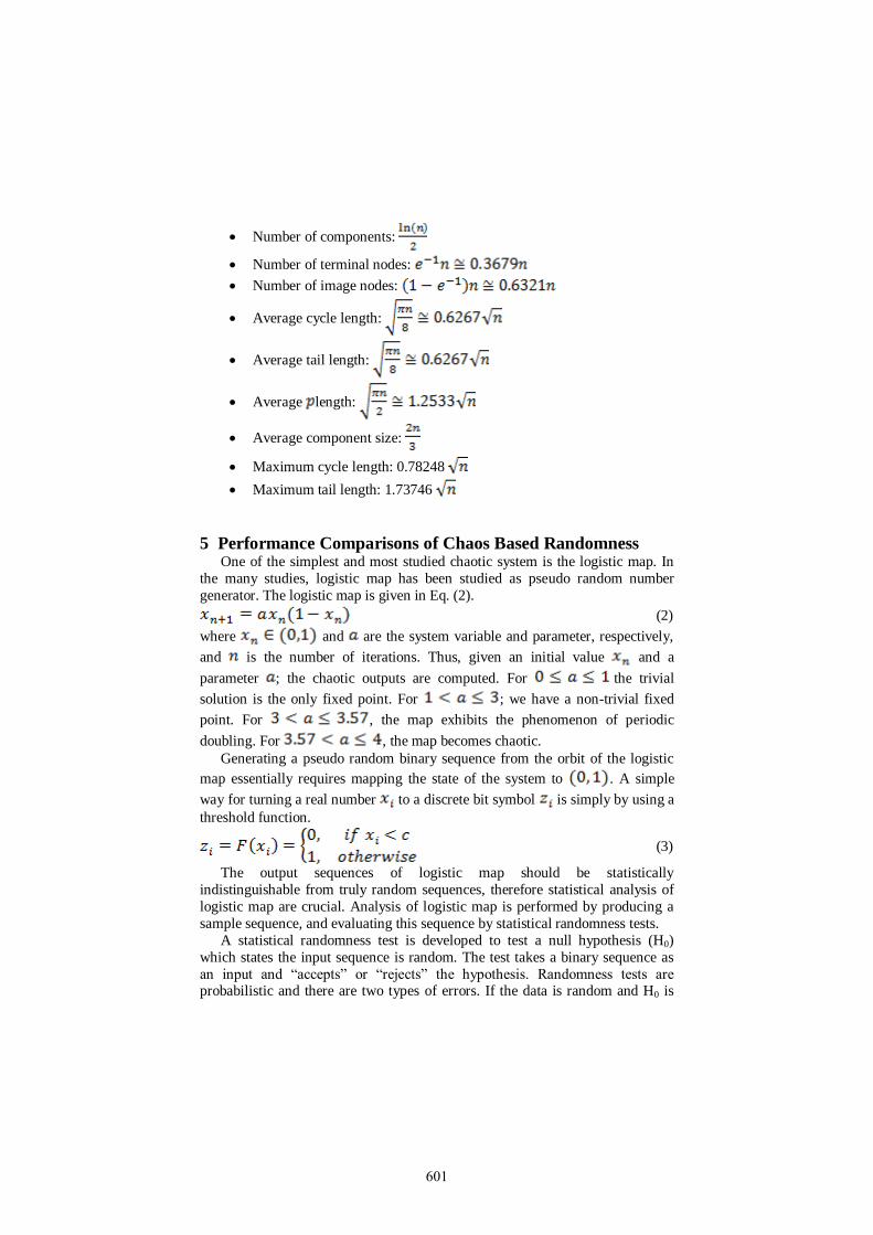
Fig. 3. Functional Graph

In Figure 3, the typical behavior of an iteration operation is given. Since the

set is finite, after some iterations, we will encounter a point that has occurred

before. Let be the point that the iteration enters a

loop. Then, , is the smallest positive integer

which we call the cycle length. The path between and is called the

tail length. The sum of the tail length and cycle length is defined as the -

length. Expected values of random mappings are widely studied in the literature.

The results of the statistical behaviors of random mappings are summarized

below [2, 28-31].

600

Number of components:

Number of terminal nodes:

Number of image nodes:

Average cycle length:

Average tail length:

Average length:

Average component size:

Maximum cycle length: 0.78248

Maximum tail length: 1.73746

5 Performance Comparisons of Chaos Based Randomness One of the simplest and most studied chaotic system is the logistic map. In

the many studies, logistic map has been studied as pseudo random number

generator. The logistic map is given in Eq. (2).

(2)

where and are the system variable and parameter, respectively,

and is the number of iterations. Thus, given an initial value and a

parameter ; the chaotic outputs are computed. For the trivial

solution is the only fixed point. For ; we have a non-trivial fixed

point. For , the map exhibits the phenomenon of periodic

doubling. For , the map becomes chaotic.

Generating a pseudo random binary sequence from the orbit of the logistic

map essentially requires mapping the state of the system to . A simple

way for turning a real number to a discrete bit symbol is simply by using a

threshold function.

(3)

The output sequences of logistic map should be statistically

indistinguishable from truly random sequences, therefore statistical analysis of

logistic map are crucial. Analysis of logistic map is performed by producing a

sample sequence, and evaluating this sequence by statistical randomness tests.

A statistical randomness test is developed to test a null hypothesis (H0)

which states the input sequence is random. The test takes a binary sequence as

an input and “accepts” or “rejects” the hypothesis. Randomness tests are probabilistic and there are two types of errors. If the data is random and H0 is

601

rejected type I error is occurred and if the data is nonrandom and H0 is accepted

type II error is occurred. The probability of a type I error is called the level of

significance of the test and denoted by . A statistical test produces a real

number between 0 and 1 which is called p-value. If p-value > then H0 is

accepted, otherwise rejected.

A test suite is a collection of statistical randomness test that are designed to

test the randomness properties of sequences. There are several test suites in the

literature:

The first collection of randomness tests were presented by Knuth in his

famous book [32].

CRYPT-X, a test suite developed in Queensland University of

Technology [33].

DIEHARD Test Suite was developed by Marsaglia and published in

1995 on a CDROM [34].

TESTU01 is a recently designed test suite, which has two categories: Those that apply to a sequence of real numbers in (0, 1) and those

designed for a sequence of bits [35].

NIST Test Suite originally consisted of 16 tests [36]. The randomness

tests in the suite are Frequency Test, Frequency Test within a Block,

Runs Test, Test for the Longest Run of Ones in a Block, Binary Matrix

Rank Test, Discrete Fourier Transform Test, Non-overlapping

Template Matching Test, Overlapping Template Matching Test,

Maurer’s Universal Statistical Test, Lempel-Ziv Compression Test,

Linear Complexity Test, Approximate Entropy Test, Cumulative Sums

Test, Random Excursions Test, and Random Excursions Variant Test.

NIST Test Suite has been used in this study to assess randomness. The

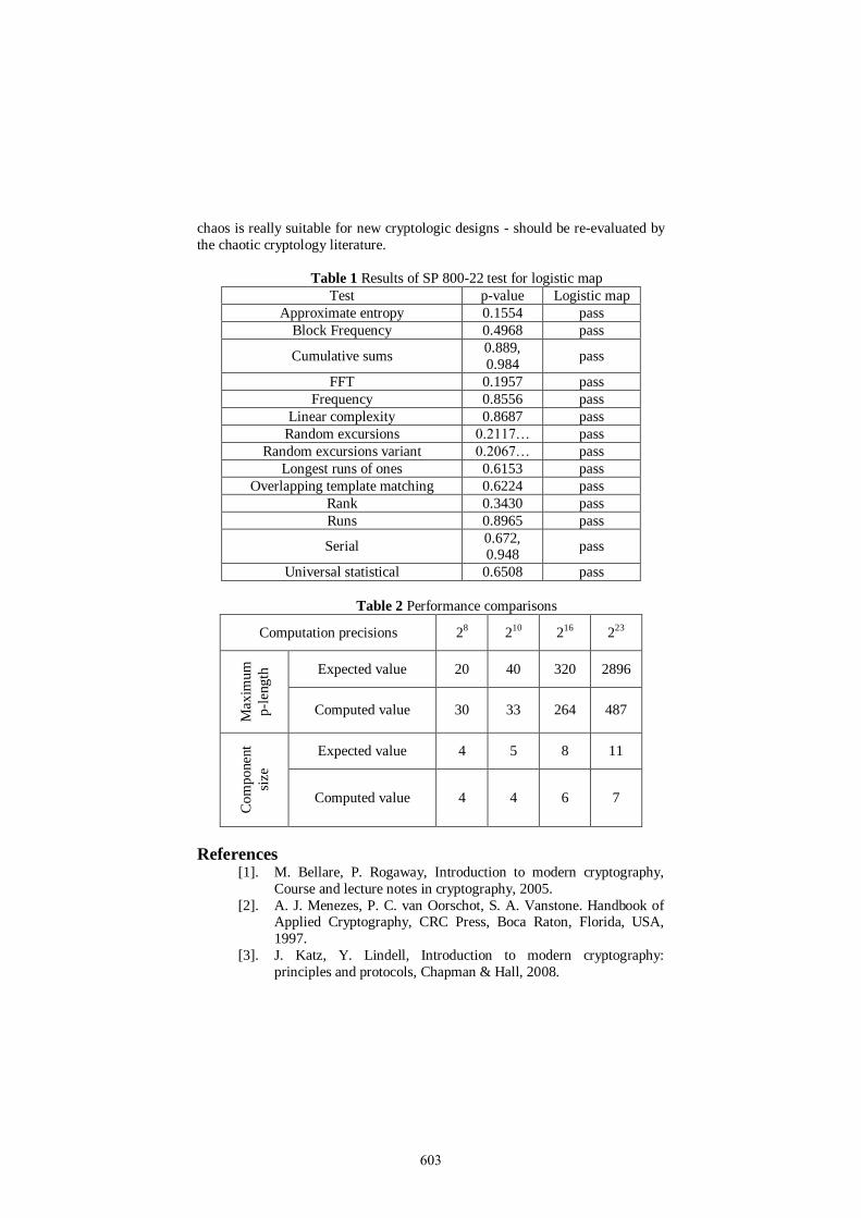
obtained results are shown in Table 1.

Calculated and expected values of random functions, obtained by using

chaotic logistic map, are given in Table 2 for different computation precision

values n. As can be seen from the table, calculated values are fewer than the

expected values for chaos based random function. These results show that even

though digital chaos based functions can pass the statistical tests, they are not fit

to be used for cryptologic randomness

6 Conclusions As a result of the analysis studies, it is determined that security of the chaos

based cryptographic designs typically analyzed by using statistical tests alone.

A common misconception, that the successful statistical test results are enough

to analyze the security of a cryptologic system, is the most important problem in

this area. To remove this misconception, the deficiencies of the statistical tests are investigated. It is revealed that, although chaotic outputs successfully pass

the standard statistical tests their randomness properties are worse than any

standard random function. Consequently, the question - whether numerical

602

chaos is really suitable for new cryptologic designs - should be re-evaluated by

the chaotic cryptology literature.

Table 1 Results of SP 800-22 test for logistic map

Test p-value Logistic map

Approximate entropy 0.1554 pass

Block Frequency 0.4968 pass

Cumulative sums 0.889,

0.984 pass

FFT 0.1957 pass

Frequency 0.8556 pass

Linear complexity 0.8687 pass

Random excursions 0.2117… pass

Random excursions variant 0.2067… pass

Longest runs of ones 0.6153 pass

Overlapping template matching 0.6224 pass

Rank 0.3430 pass

Runs 0.8965 pass

Serial 0.672, 0.948

pass

Universal statistical 0.6508 pass

Table 2 Performance comparisons

Computation precisions 28 210 216 223

Max

imu

m

p-l

eng

th Expected value 20 40 320 2896

Computed value 30 33 264 487

Co

mp

onen

t

size

Expected value 4 5 8 11

Computed value 4 4 6 7

References [1]. M. Bellare, P. Rogaway, Introduction to modern cryptography,

Course and lecture notes in cryptography, 2005.

[2]. A. J. Menezes, P. C. van Oorschot, S. A. Vanstone. Handbook of Applied Cryptography, CRC Press, Boca Raton, Florida, USA,

1997.

[3]. J. Katz, Y. Lindell, Introduction to modern cryptography:

principles and protocols, Chapman & Hall, 2008.

603

[4]. C. Paar, J. Pelzl, Understanding Cryptography A Textbook for

Student and Practitioners, Springer, 2010.

[5]. J. Sprott, Elegant Chaos Algebraically Simple Chaotic Flows.

World Scientific, 2010.

[6]. J. M. Amigo, L. Kocarev, J. Szczapanski, Theory and practice of chaotic cryptography, Physics Letters A 366 (2007) 211-216.

[7]. G. Alvarez, S. Li, Some basic cryptographic requirements for

chaos-based cryptosystems. International Journal of Bifurcation

and Chaos 16/8 (2006) 2129–2151

[8]. E. Solak, Cryptanalysis of Chaotic Ciphers, in: L. Kocarev, S. Lian

(Eds.), Chaos Based Cryptography Theory Algorithms and

Applications, Springer-Verlag (2011) 227-256.

[9]. G. Alvarez, J. M. Amigo, D. Arroyo, S. Li, Lessons Learnt from

the Cryptanalysis of Chaos-Based Ciphers, in: L. Kocarev, S. Lian

(Eds.), Chaos Based Cryptography Theory Algorithms and

Applications, Springer-Verlag (2011) 257-295.

[10]. X. Wang, W. Zhang, W. Guo, Jiashu Zhang, Secure chaotic system with application to chaotic ciphers, Information Sciences 221

(2013) 555-570.

[11]. A. Kanso, H. Yahyaoui, M. Almulla, Keyed hash function based

on a chaotic map, Information Sciences 186/1 (2012) 249-264.

[12]. C. Chen, C. Lin, C. Chiang, S. Lin, Personalized information

encryption using ECG signals with chaotic functions, Information

Sciences 193 (2012) 125-140.

[13]. Z. Zhu, W. Zhang, K. Wong, H. Yu, A chaos-based symmetric

image encryption scheme using a bit-level permutation,

Information Sciences 181/6 (2011) 1171-1186.

[14]. .J. Fridrich, Symmetric ciphers based on two-dimensional chaotic maps, International Journal of Bifurcation and Chaos 8/6 (1998)

1259–1284.

[15]. C. Zhu, A novel image encryption scheme based on improved

hyperchaotic sequences, Optics Communications 285/1 (2012) 29-

37

[16]. H. Hu, L. Liu, N. Ding, Pseudorandom sequence generator based

on Chen chaotic system, Computer Physics Communications 184

(2013) 765–768.

[17]. Q. Zhang, L. Guo, X. Wei, Image encryption using DNA addition

combining with chaotic maps, Mathematical and Computer

Modelling 52 (2010) 2028-2035.

[18]. N. Bigdeli, Y. Farid, K. Afshar, A robust hybrid method for image encryption based on Hopfield neural network, Computers and

Electrical Engineering 38, pp.356–369, 2012.

[19]. L. Liu, Q. Zhang, X. Wei, A RGB image encryption algorithm

based on DNA encoding and chaos map, Computers & Electrical

Engineering, 38/5 (2012) 1240-1248.

604

[20]. F. Özkaynak, S. Yavuz, Security problems of pseudorandom

sequence generator based on Chen chaotic system, Computer

Physics Communications 184 (2013) 2178–2181.

[21]. F. Özkaynak, A. B. Özer, S. Yavuz, Cryptanalysis of a novel

image encryption scheme based on improved hyperchaotic sequences, Optics Communications 285 (2012) 4946–4948.

[22]. F. Özkaynak, A. B. Özer, S. Yavuz, Cryptanalysis of Bigdeli

algorithm using Çokal and Solak attack, International Journal of

Information Security Science, 1/3 (2012) 79-81.

[23]. F. Özkaynak, A. B. Özer, S. Yavuz, (2012). Analysis of Chaotic

Methods for Compression and Encryption Processes in Data

Communication, 20th IEEE Signal Processing and

Communications Applications Conference.

[24]. F. Özkaynak, A. B. Özer, S. Yavuz, (2013). Security Analysis of

An Image Encryption Algorithm Based on Chaos and DNA

Encoding, 21th IEEE Signal Processing and Communications

Applications Conference. [25]. E. Solak, C. Çokal , Algebraic break of image ciphers based on

discretized chaotic map lattices, Information Sciences, 181/1

(2011) ,227-233

[26]. E. Solak, C. Çokal, O.T. Yildiz, T. Biyikoglu, Cryptanalysis of

fridrich’s chaotic image encryption. International Journal of

Bifurcation and Chaos 20/5 (2010) 1405–1413.

[27]. F. Özkaynak, S. Yavuz, Analysis and improvement of a novel

image fusion encryption algorithm based on DNA sequence

operation and hyper-chaotic system, Nonlinear Dynamics:

Volume, 78/2, 1311-1320, 2014.

[28]. P. Flajolet, A. M. Odlyzko, Random mapping statistics, In EUROCRYPT (1989) 329–354.

[29]. B. Harris, Probability distributions related to random mappings.

The Annals of Mathematical Statistics 31/4 (1960) 1045–1062.

[30]. V. F. Kolchin. Random Mappings. Springer-Verlag, 1986.

[31]. J. Arney, E. A. Bender, Random mappings with constraints on

coalescence and number of origins, Pacific J. Math. 103/2

(1982)269–294.

[32]. D. E. Knuth, Seminumerical Algorithms, volume 2 of The Art of

Computer Programming, Addison-Wesley, 1981.

[33]. W. Caelli, E. Dawson, L. Nielsen, H. Gustafson, CRYPT–X

statistical package manual, measuring the strength of stream and

block ciphers, 1992. [34]. G. Marsaglia, The Marsaglia random number CDROM including

the DIEHARD battery of tests of randomness, 1996.

[35]. P. L’Ecuyer, R. Simard, Testu01: A c library for empirical testing

of random number generators. ACM Trans. Math. Softw., 33/4

(2007) 22.

605

[36]. A. Rukhin, J. Soto, J. Nechvatal, M. Smid, E. Barker, S. Leigh, M.

Levenson, M. Vangel, D. Banks, A. Heckert, J. Dray, S. Vo, A

statistical test suite for random and pseudorandom number

generators for cryptographic applications, 2001.

[37]. F. Özkaynak, Cryptographically secure random number generator with chaotic additional input, Nonlinear Dynamics, 78/3, 2015-

2020, 2014.

606

_________________

8th

CHAOS Conference Proceedings, 26-29 May 2015, Henri Poincaré Institute, Paris France

© 2015 ISAST

Entropy Analysis with Lyapunov Exponents for

Random Number Generators

Fatih Özkaynak1, Ahmet Bedri Özer2

1 Fırat University, Department of Software Engineering, 23119 Elazig, Turkey

(E-mail: ozkaynak_fatih@hotmail.com) 2

Fırat University, Department of Computer Engineering, 23119 Elazig, Turkey

(E-mail: bedriozer@firat.edu.tr)

Abstract. Many applications require random numbers. Generating high quality random numbers is a very serious problem. It is quite easy to design a random number generator that will pass the statistical tests, but it is much more difficult to know where the randomness comes from and how much true randomness is there. Chaotic system is regarded as an important entropy source in the design of random number generator. The

relationship between random number generator and chaotic dynamical systems is studied in this paper. The main contribution of this paper is that it gives an analysis method for entropy source in random number generators. Entropy describes the unpredictability of random number generators. In practice, calculation of entropy is hard, so Lyapunov exponent has been used as an unpredictability measure of entropy source. Proposed analysis method has been verified on a chaos based random number generator design, and fits to analysis of other RNG designs. Keywords: Random number generator, Entropy, Lyapunov Exponent, Chaos.

1 Introduction A random number generator (RNG) produces a sequence of random (or

random-looking) numbers in a predetermined range, such as r_i∈0,1 or

r_i∈[0,1]. Random numbers have many applications: statistical physics,

simulation, industrial testing and labeling, games, gambling, Monte Carlo

methods, and cryptography [1, 2].

Generating high quality random numbers is a very serious problem. The

random numbers should assume all admissible values with equal probability and

should be independent from predecessors and successors. This characterizes an

ideal RNG. In an ideal RNG, even with maximal knowhow and unlimited

computational power an attacker has no better strategy blind guessing. Guessing

n random bits costs 2^(n-1) trials in average. The guess work remains invariant in the course of the time. However, an ideal RNG is a mathematical construct.

There are two basic categories of RNGs: True RNGs and Deterministic RNGs.

It is quite easy to design a RNG that will pass the statistical tests, but it is much

more difficult to know where the randomness comes from and how much true

randomness is there [2-5].

The most striking feature of RNGs is the unpredictability of the past and

future random numbers from some subsequent random numbers.

607

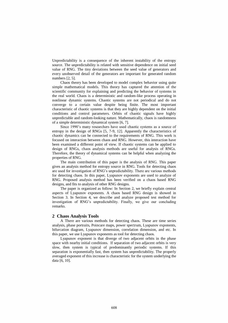
Unpredictability is a consequence of the inherent instability of the entropy

source. The unpredictability is related with sensitive dependence on initial seed

value of RNG. The tiny deviations between the seed value of generators and

every unobserved detail of the generators are important for generated random

numbers [2, 5]. Chaos theory has been developed to model complex behavior using quite

simple mathematical models. This theory has captured the attention of the

scientific community for explaining and predicting the behavior of systems in

the real world. Chaos is a deterministic and random-like process operating in

nonlinear dynamic systems. Chaotic systems are not periodical and do not

converge to a certain value despite being finite. The most important

characteristic of chaotic systems is that they are highly dependent on the initial

conditions and control parameters. Orbits of chaotic signals have highly

unpredictable and random-looking nature. Mathematically, chaos is randomness

of a simple deterministic dynamical system [6, 7].

Since 1990’s many researchers have used chaotic systems as a source of

entropy in the design of RNGs [5, 7-9, 12]. Apparently the characteristics of chaotic dynamics can be connected to the requirements of RNG. This work is

focused on interaction between chaos and RNG. However, this interaction have

been examined a different point of view. If chaotic systems can be applied to

design of RNGs, chaos analysis methods are useful for analysis of RNGs.

Therefore, the theory of dynamical systems can be helpful when analyzing the

properties of RNG.

The main contribution of this paper is the analysis of RNG. This paper

gives an analysis method for entropy source in RNG. Tools for detecting chaos

are used for investigation of RNG’s unpredictability. There are various methods

for detecting chaos. In this paper, Lyapunov exponents are used to analyze of

RNG. Proposed analysis method has been verified on a chaos based RNG designs, and fits to analysis of other RNG designs.

The paper is organized as follow: In Section 2, we briefly explain central

aspects of Lyapunov exponents. A chaos based RNG design is showed in

Section 3. In Section 4, we describe and analyze proposed test method for

investigation of RNG’s unpredictability. Finally, we give our concluding

remarks.

2 Chaos Analysis Tools A There are various methods for detecting chaos. These are time series

analysis, phase portraits, Poincare maps, power spectrum, Lyapunov exponents,

bifurcation diagram, Lyapunov dimension, correlation dimension, and etc. In

this paper, we use Lyapunov exponents as tool for detecting chaos.

Lyapunov exponent is that diverge of two adjacent orbits in the phase

space with nearby initial conditions. If separation of two adjacent orbits is very

slow, then system is typical of predominantly periodic systems. If this

separation is exponentially fast, then system has unpredictability. The properly averaged exponent of this increase is characteristic for the system underlying the

data [6, 10].

608

Calculation of the Lyapunov exponent is conceptually simple since one

only needs to follow two initially nearby trajectories and fit the logarithm of

their separation to a linear function of time. The slope of the fit is the Lyapunov

exponent. Let and be two points in state space with distance

. Denote by the distance some time ahead

between the two trajectories emerging from these points, .

Then λ is determined by Eq. (1) [6, 10].

(1)

If λ is positive, this means an exponential divergence of nearby

trajectories with nearby initial conditions. A negative maximal Lyapunov

exponent reflects the existence of a stable fixed point. Two adjacent orbits

which approach the fixed point also approach each other exponentially fast. If

the motion settles down onto a limit cycle, two adjacent orbits can only separate

or approach each other slower than exponentially. In this case the maximal

Lyapunov exponent is zero and the motion is called marginally stable. If a predominantly deterministic system is perturbed by random noise, on the small

scales it can be characterized by a diffusion process, with n growing as n. Thus

the maximal Lyapunov exponent is infinite. General characteristics of Lyapunov

exponent is given in Table 1 [6, 10].

Table 1. General characteristics of Lyapunov exponent

Type of motion Maximal Lyapunov exponent

stable fixed point λ < 0

stable limit cycle λ = 0

chaos 0 < λ < ∞

noise λ=∞

3 A Chaos Based RNG Logistic map is one of the simplest and most studied nonlinear system in

the design of RNGs. The logistic map is defined as Eq. (2).

(2)

Structure in Eq. (3) has been used to convert the iterations of a logistic

map into binary digits is by defining a function .

(3)

where is a threshold value taken to be 0.5 to ensure approximately equal

distributions of 0’s and 1’s in the sequence . Furthermore, for c = 0.5, the

generated sequences have been demonstrated to possess good statistical

distribution properties. The most comprehensive statistical test suite, NIST test

suite [11], was applied to test such sequences, and the results turned out to be

very satisfactory.

609

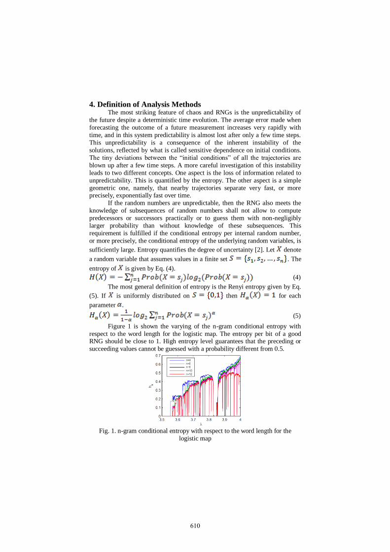
4. Definition of Analysis Methods The most striking feature of chaos and RNGs is the unpredictability of

the future despite a deterministic time evolution. The average error made when

forecasting the outcome of a future measurement increases very rapidly with

time, and in this system predictability is almost lost after only a few time steps.

This unpredictability is a consequence of the inherent instability of the

solutions, reflected by what is called sensitive dependence on initial conditions.

The tiny deviations between the “initial conditions” of all the trajectories are

blown up after a few time steps. A more careful investigation of this instability

leads to two different concepts. One aspect is the loss of information related to

unpredictability. This is quantified by the entropy. The other aspect is a simple

geometric one, namely, that nearby trajectories separate very fast, or more precisely, exponentially fast over time.

If the random numbers are unpredictable, then the RNG also meets the

knowledge of subsequences of random numbers shall not allow to compute

predecessors or successors practically or to guess them with non-negligibly

larger probability than without knowledge of these subsequences. This

requirement is fulfilled if the conditional entropy per internal random number,

or more precisely, the conditional entropy of the underlying random variables, is

sufficiently large. Entropy quantifies the degree of uncertainty [2]. Let denote

a random variable that assumes values in a finite set . The

entropy of is given by Eq. (4).

(4)

The most general definition of entropy is the Renyi entropy given by Eq.

(5). If is uniformly distributed on then for each

parameter .

(5)

Figure 1 is shown the varying of the n-gram conditional entropy with

respect to the word length for the logistic map. The entropy per bit of a good RNG should be close to 1. High entropy level guarantees that the preceding or

succeeding values cannot be guessed with a probability different from 0.5.

Fig. 1. n-gram conditional entropy with respect to the word length for the

logistic map

610

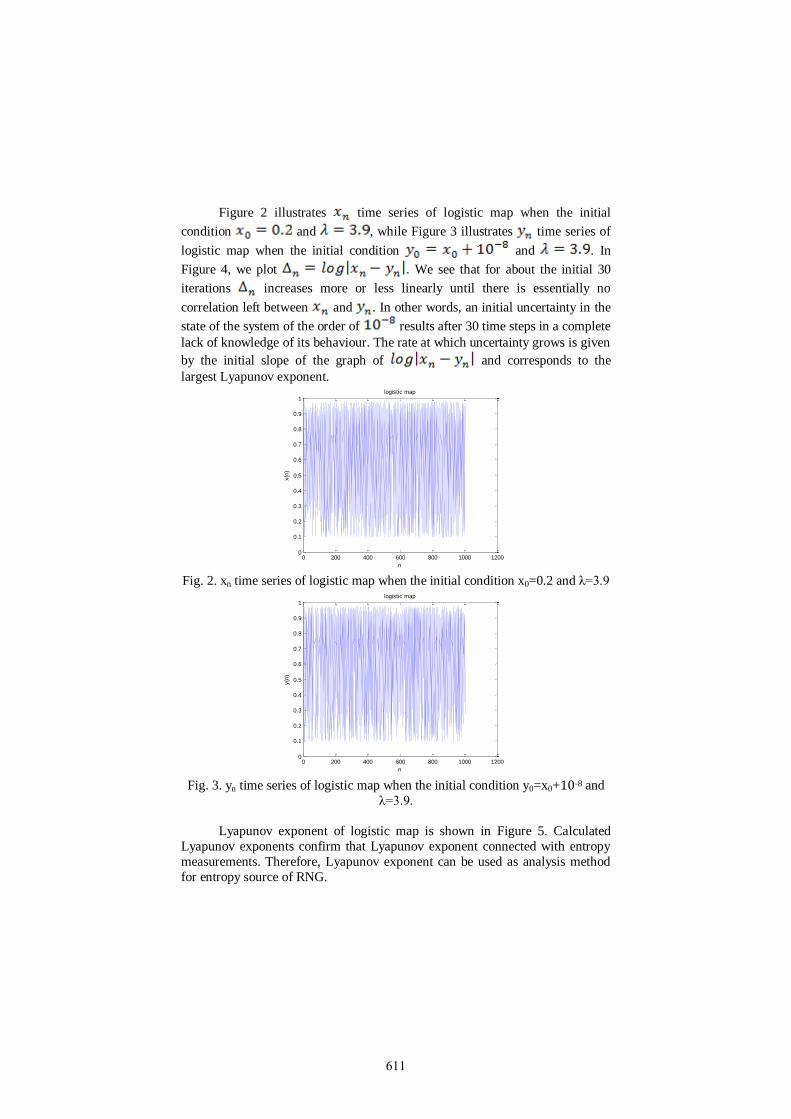
Figure 2 illustrates time series of logistic map when the initial

condition and , while Figure 3 illustrates time series of

logistic map when the initial condition and . In

Figure 4, we plot . We see that for about the initial 30

iterations increases more or less linearly until there is essentially no

correlation left between and . In other words, an initial uncertainty in the

state of the system of the order of results after 30 time steps in a complete

lack of knowledge of its behaviour. The rate at which uncertainty grows is given

by the initial slope of the graph of and corresponds to the

largest Lyapunov exponent.

0 200 400 600 800 1000 12000

0.1

0.2

0.3

0.4

0.5

0.6

0.7

0.8

0.9

1logistic map

n

x(n

)

Fig. 2. xn time series of logistic map when the initial condition x0=0.2 and λ=3.9

0 200 400 600 800 1000 12000

0.1

0.2

0.3

0.4

0.5

0.6

0.7

0.8

0.9

1logistic map

n

y(n

)

Fig. 3. yn time series of logistic map when the initial condition y0=x0+10-8 and

λ=3.9.

Lyapunov exponent of logistic map is shown in Figure 5. Calculated

Lyapunov exponents confirm that Lyapunov exponent connected with entropy

measurements. Therefore, Lyapunov exponent can be used as analysis method

for entropy source of RNG.

611

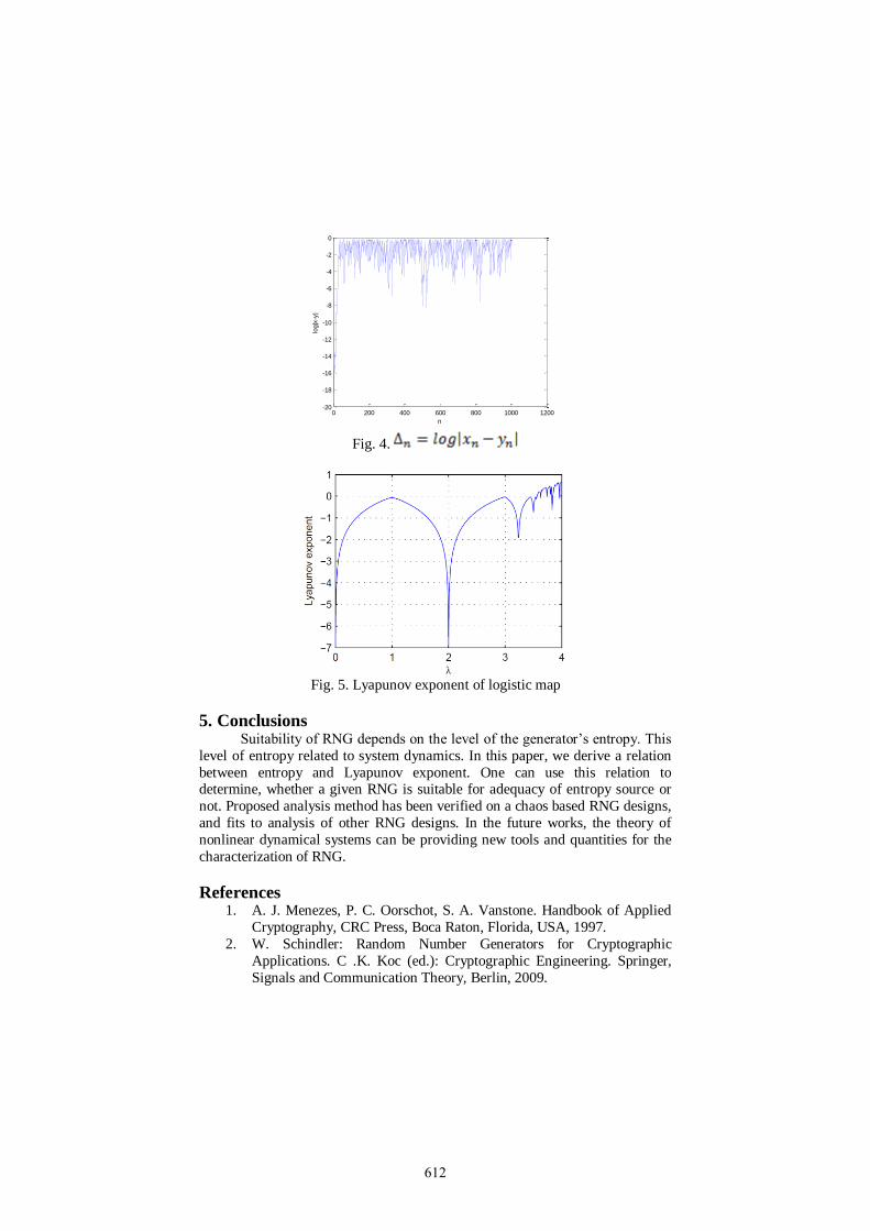
0 200 400 600 800 1000 1200-20

-18

-16

-14

-12

-10

-8

-6

-4

-2

0

n

log|x

-y|

Fig. 4.

Fig. 5. Lyapunov exponent of logistic map

5. Conclusions Suitability of RNG depends on the level of the generator’s entropy. This

level of entropy related to system dynamics. In this paper, we derive a relation

between entropy and Lyapunov exponent. One can use this relation to determine, whether a given RNG is suitable for adequacy of entropy source or

not. Proposed analysis method has been verified on a chaos based RNG designs,

and fits to analysis of other RNG designs. In the future works, the theory of

nonlinear dynamical systems can be providing new tools and quantities for the

characterization of RNG.

References 1. A. J. Menezes, P. C. Oorschot, S. A. Vanstone. Handbook of Applied

Cryptography, CRC Press, Boca Raton, Florida, USA, 1997.

2. W. Schindler: Random Number Generators for Cryptographic

Applications. C .K. Koc (ed.): Cryptographic Engineering. Springer,

Signals and Communication Theory, Berlin, 2009.

612

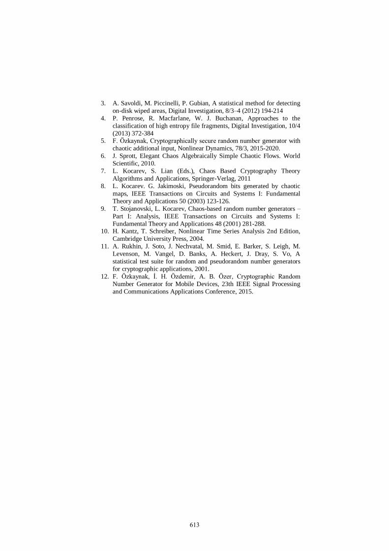
3. A. Savoldi, M. Piccinelli, P. Gubian, A statistical method for detecting

on-disk wiped areas, Digital Investigation, 8/3–4 (2012) 194-214

4. P. Penrose, R. Macfarlane, W. J. Buchanan, Approaches to the

classification of high entropy file fragments, Digital Investigation, 10/4

(2013) 372-384 5. F. Özkaynak, Cryptographically secure random number generator with

chaotic additional input, Nonlinear Dynamics, 78/3, 2015-2020.

6. J. Sprott, Elegant Chaos Algebraically Simple Chaotic Flows. World

Scientific, 2010.

7. L. Kocarev, S. Lian (Eds.), Chaos Based Cryptography Theory

Algorithms and Applications, Springer-Verlag, 2011

8. L. Kocarev. G. Jakimoski, Pseudorandom bits generated by chaotic

maps, IEEE Transactions on Circuits and Systems I: Fundamental

Theory and Applications 50 (2003) 123-126.

9. T. Stojanovski, L. Kocarev, Chaos-based random number generators –

Part I: Analysis, IEEE Transactions on Circuits and Systems I:

Fundamental Theory and Applications 48 (2001) 281-288. 10. H. Kantz, T. Schreiber, Nonlinear Time Series Analysis 2nd Edition,

Cambridge University Press, 2004.

11. A. Rukhin, J. Soto, J. Nechvatal, M. Smid, E. Barker, S. Leigh, M.

Levenson, M. Vangel, D. Banks, A. Heckert, J. Dray, S. Vo, A

statistical test suite for random and pseudorandom number generators

for cryptographic applications, 2001.

12. F. Özkaynak, İ. H. Özdemir, A. B. Özer, Cryptographic Random

Number Generator for Mobile Devices, 23th IEEE Signal Processing

and Communications Applications Conference, 2015.

613

614

Simulation of Multidimensional NonlinearDynamics by One-Dimensional Maps with

Many Parameters

Irina N. Pankratova1 and Pavel A. Inchin2

1 Institute of Mathematics and Mathematical Modeling, Dep. of DifferentialEquations, 050010 Pushkin str., 125, Almaty, Kazakhstan(E-mail: inpankratova@gmail.com)

2 Institute of Mathematics and Mathematical Modeling, Dep. of DifferentialEquations, 050010 Pushkin str., 125, Almaty, Kazakhstan(E-mail: paul.inchin@yahoo.com)

Abstract. We propose a concrete class of discrete dynamical systems as nonlinearmatrix models to describe the multidimensional multiparameter nonlinear dynamics.In this article we simulate the system asymptotic behavior. A two-step algorithm forthe computation of ω-limit sets of the dynamical systems is presented. In accordancewith the qualitative theory which we develop for this class of systems, we allocateinvariant subspaces of the system matrix containing cycles of rays on which ω-limitsets of the dynamical systems are situated and introduce the dynamical parametersby which the system behavior is described in the invariant subspaces. As the firststep of the algorithm, a cycle of rays which contains the ω-limit set of the systemtrajectory, is allocated using system matrix. As the second step, the ω-limit set of thesystem trajectory is computed using the analytical form of one-dimensional nonlinearPoincare map dependent on the dynamical parameters. The proposed algorithmsimplifies calculations of ω-limit sets and therefore reduces computing time. A graphicvisualization of ω- limit sets of n- dimensional dynamical systems, n > 3 is shown.Keywords: Computer simulation, Nonlinear dynamics, Discrete dynamical systems,Dynamical parameters.

1 Introduction

To understand and analyse nonlinear multidimensional dynamics simple one-dimensional semi-dynamical systems with complicated dynamics and fairlycomplete qualitative description are used. These are, first of all, one-dimensionaldiscrete dynamical systems, i.e. iterations of real one-dimensional maps. Thefirst systematic results on one-dimensional discrete dynamical systems ap-peared in the early 60’s and are linked to A.N. Sharkovskii [1]. Many propertiesof the dynamical systems are the direct result of the theories developed by A.N.Sharkovskii [2] and M. Feigenbaum [3]. A representative of this class of sys-tems is the dynamical system generated by the one-dimensional logistic map

8thCHAOS Conference Proceedings, 26-29 May 2015, Henri Poicare Institute,Paris France

c© 2015 ISAST

615

[4]. It was the first example of a complicated, chaotic behaviour of the systemgiven by a simple nonlinear equation. Even though the properties of the one-dimensional logistic map are well studied, researchers continue referring to itas standard to check the many nonlinear phenomena [5]–[7]. However, up untilnow there is no well-developed qualitative theory available, which could be suc-cessfully applied in order to conduct a complete study of the multidimensionaldynamical systems dependent on parameters. Therefore, it is appropriate toselect concrete classes of the dynamical systems and to develop qualitative the-ories so as to be able to describe the properties and movements of the systemswithin these theories.

We focus our research on a concrete class of dynamical systems which repre-sent a variant of generalization of one-dimensional discrete dynamical systemsto the multidimensional multiparameter case. The systems are generated by amap in the form of the product of scalar and vector linear functions on compactsets of the real vector space. We propose the systems as nonlinear matrix mod-els with limiting factors to describe the macro system dynamics, for examplethe dynamics of many group biological population in the presence of limitedresources. In these models the scalar function plays a role of a limiting factor.

In recent years, the methods of computer simulation have become an essen-tial tool in the study of the dynamical systems [8]–[10]. The modern computercapabilities make it possible to include in the system complicated nonlinearrelationships between its variables and a large number of parameters. Thepresence of nonlinear relationships and multiparameter dependence reproducesin the model the phenomena which can be observed in actual experiments andwhich cannot be produced by splitting the system into separate componentsor reducing the number of parameters or variables. Thus, the improvement ofcurrent methods and the development of new ones for the dynamical systemresearch are necessary and relevant [11,12]. In this case the quantitative re-search provides a theoretical basis for the algorithm constructions, and henceis particularly important.

We develop a qualitative theory for the class of the dynamical systemsconsidered (see e.g. [13] and references there). The systems possess the obvi-ous properties which are determined by the linear vector function (the systemmatix) and which do not depend on the scalar function. In particular, in vectorspace we allocate invariant subspaces containing cycles of rays of the systemmatrix, on which ω-limit sets of dynamical systems are situated. On the otherhand, the complicated nonlinear dynamics of the systems can occur due tothe scalar function. We study the system dynamics in the invariant subspacescontaining cycles of rays using one-dimensional nonlinear Poincare maps andintroduce the dynamical parameters by which the system behavior is describedin the invariant subspaces. In this article we show the results of the simulationof the system asymptotic behavior and present an algorithm for the compu-tation of ω-limit sets of the class of the dynamical systems considered. Thealgorithm consists of two steps of calculations in accordance with the qualita-tive theory. As the first step, a cycle of rays which contains the ω-limit setof the system trajectory is allocated using system matrix. The period of thecycle of rays, the number and values of the dynamical parameters by which the

616

system dynamics is described on the cycle of rays, are calculated as well. Asthe second step, the ω-limit set of the system trajectory is computed using one-dimensional nonlinear Poincare map dependent on the dynamical parameters.As a rule, these parameters differ from the system parameters and are unknownor not directly defined or computable [14]. The novelty of our research lies inthe determination of the dynamical parameters and in the analytical form ofone-dimensional nonlinear Poincare maps dependent on the dynamical param-eters. We shall see below that the number of the dynamical parameters cannotbe reduced without the loss of accuracy of the system behavior description,even when this number is greater than the number of the system parameters,i.e. entries of the system matrix.

2 Class of the dynamical systems

Let F be a map of the form [13]

F : Rn → Rn, Fy = Φ(y)Ay (1)

where Rn is n- dimensional real vector-space, Φ(y) is a scalar function, A is alinear operator (a matrix of n-th order). Allocate set X ⊆ Rn invariant underF i.e., F : X → X. Map F in general is non invertible and generates in Xa cyclic semi-group of maps Fm, m ∈ Z+, which is called the dynamicalsystem and is denoted by Fm,X, Z+. Set X is called phase space of thedynamical systems and specifies a set of valid states of the dynamical system,Z+ = N

⋃0 is the set of nonnegative integers. Set Fmy where y is fixed

and m runs over Z+, is called a trajectory of the point y. The dynamics of thesystem Fm,X, Z+ is understood as the process of transition from one stateto another.

The dynamics of the system Fm,X, Z+ generally varies for different Φ(y).So, the systems Fm,X, Z+ are different too. But the systems possess similarproperties which are determined by the linear operator A and do not dependon the function Φ(y). Therefore, the systems Fm,X, Z+ form one class ofthe dynamical systems.The elements of this class are, in particular, linear dy-namical systems with Φ(y) = const and the dynamical system fm,X, Z+generated by the map f of the form [15]

f : Rn → Rn, fy = (1− ‖y‖)Ay. (2)

Here ‖ · ‖ is a vector norm in Rn. If n = 1 then A = µ and we arrive at thewell-known logistic map mentioned above

ψµ : R1 → R1, ψµx = µ(1− x)x. (3)

3 Mathematical models with limiting factors

We propose the class of the dynamical systems Fm,X, Z+ as mathematicalmodels for describing the dynamics of model and real macro systems in thepresence of limiting factors.

617

Letn be a number of macro system’s components,y ∈ X be a vector of components’ characteristics,A be a matrix of components’ interrelations andΦ(y) be a limiting function (limiting factor).

Let X be a compact of the form

X = y ∈ Rn | y ≥ 0, ‖y‖ ≤ a, a <∞. (4)

Here y = (y1, . . . , yn)′ ≥ 0 means yi ≥ 0, i = 1, n and is called a nonnegativevector. Note that X is invariant under F i.e., F : X→ X if and only if [13]1) Φ(y) ≥ 0 is continuous function on X,2) A = (aij) ≥ 0 (aij ≥ 0, i, j = 1, n),3) ‖A‖ ≤ aC−1 where C = max

y∈XΦ(y)‖y‖ and ‖A‖ is a subordinate matrix norm

for a matrix A based on the vector norm in Rn.Then the dynamical system Fm,X, Z+ describes the macro system’s state

changes over time m. For any nontrivial Fmy we introduce a unit vector

em(y) = ‖Fmy‖−1Fmy (5)

which is called a macro system structure and defines the ratio between compo-nents’ characteristics at the time m. The state of macro system governed bythe dynamical system Fm,X, Z+ (at the time m) we characterize by

Sm(y) = Fmy, em(y). (6)

The limiting factor concept was first coined in biology by Libig J. andgenerally, means a factor that restricts or constrains the dynamics of the system,process or phenomena. By using limiting factors, the state of the system isregulated.

On one hand, models given by the systems Fm,X, Z+ generalize in n- di-mensional case many nonlinear one- and two-dimensional models widely usedin practice. In particular, for describing the dynamics of n- group biologicalpopulation with discrete generations in the presence of limited resources wepropose the dynamical system generated by the map f of the form (2). In thisrepresentation y is a vector of densities of population age groups so, ‖y‖ ≤ 1.If n = 1 then y is the total population density, A ≡ µ is the reproductive coeffi-cient. The dynamical system ψmµ , I, Z+ in the interval I1 = [0, 1] describes amechanism of self-regulation of one-species biological population with limitedresources [2].

On the other hand, models given by the systems Fm,X, Z+ generalizemany matrix models, in particular, Leslie models both linear and nonlinear[16,17]. The last ones contain matrices A of the special form (Leslie matrixand its generalizations) and concrete limiting functions Φ(y).

4 Qualitative theory

We develop a qualitative theory for the class of the dynamical systems Fm,X, Z+and apply the results of the theory in computer simulation of their dynamics.

618

Denote by ωF y ω- limit set of the trajectory Fmy (the set which attractsFmy when m → +∞). A ray passing through y ∈ Rn, y 6= 0 is the setcone(y) = αy | α ≥ 0. By a system of p elements we mean a sequence ofthese elements, p ∈ N. Then the system of distinct rays l1, ..., lp is called a cycleof rays of a linear operator A of period p ∈ N and is denoted by Lp = (l1, ..., lp)if

Alk = lk+1, k = 1, . . . , p− 1, Alp = l1.

As easy to see, that invariant sets of the system Fm,X, Z+ are containedin invariant subspaces of A. Denote kerA = y ∈ Rn | Ay = 0 and let

P(A; p, µ) = Ap − µpE, µ ∈ C.

We call the intersection l ∩ X as a segment of ray l (ray segment). Denote byφµ map F when n = 1,

φµx = µΦ(x)x (7)

where x ∈ Ia = [0, a]. According to the qualitative theory there exist p, q ∈ N,µ ∈ σ(A) such that any nontrivial ( 6= 0) ωF y is located in some invariantsubspace

kerP(A; p, µ), µp > 0,

on a cycle of rays Lq where σ(A) is a spectrum of A and q is a divisor of p,1 ≤ q ≤ p [18]. More precisely, ωF y ⊆ Jq = Lq ∩ X ⊂ kerP(A; p, µ) ∩ X andJq consists of q ray segments invariant under F q. Without losing generality weagree q = p and ωF y ⊆ Jp. Then for the map F with Φ(‖y‖) map F p representsin Jp as a superposition

F p = φµp φµp−1 . . . φµ1 (8)

with some numbers µ1 > 0, . . . , µp > 0.If to consider the system Fm, kerP(A; p, µ)∩X, Z+, then µ1, . . . , µp turns

into parameters. We call them dynamical parameters in contrast to the systemparameters i.e. entries of the matrix A. Thus, in the whole X, the systemdynamics is defined by the trajectory behavior in the sets kerP(A; p, µ) ∩ X.So, by the parameters µ1, . . . , µp the system dynamics is described in thewhole X. Every ray segment of Jp is the one-dimensional Poincare sectionfor the trajectories located in Jp and F p is the one-dimensional first return(Poincare) map for the map F in each ray segment of Jp. For the special formΦ(‖y‖) map F p has analytical representation (8).

Denote by e1, . . . , ep the unit vectors directed along the ray segments ofJp. We define e1, . . . , ep and µ1, . . . , µp by the recurrent formulas. Let p = 1.Then e1 ≥ 0 is an eigen vector of the matrix A ≥ 0 and there exists an eigenvalue µ > 0 such as Ae1 = µe1. So, (8) takes the form

F = φµ. (9)

Let p > 1 then e1 ≥ 0 is not an eigen vector of A, ‖e1‖ = 1 and e2, . . . , ep aredefined by the sequence

ej = ‖Aej−1‖−1Aej−1, j = 2, p. (10)

619

Denoteµj = ‖Aej‖, j = 1, p. (11)

For the map F with different Φ(‖y‖), parameters µ1, . . . , µp and vectors e1,. . . , ep are the same and their computation by the formulas (10)-(11) does notcause difficulties.

It should be noted that the dynamical parameters, their number and val-ues depend on the location of the sets kerP(A; p, µ) ∩ X in X and Jp inkerP(A; p, µ) ∩ X and vary, as a rule, at the fixed entries of the matrix A.So, the dynamical parameters differ from the system parameters and identifythe regions with different dynamics. Their number is less than or equal to pand may be very large, in particular, when p > n2 at n ≥ 19 [18]. Accordingto (8) all parameters are involved in the representation of the map F p so, theirnumber cannot be reduced.

5 Computer simulation

We present computer simulation of multidimensional dynamics by the numeri-cal realization of the models for the dynamics of biological population governedby the system fm,X, Z+.

In the population model:f is a map of the form (2): fy = (1− ‖y‖)Ay,n is a number of population age groups,y is a vector of densities of the age groups, y ∈ X,X is of the form (4) if a = 1 i.e.,

X = y ∈ Rn | y ≥ 0, ‖y‖ ≤ 1,

A is a matrix of intergroup relations,Φ(‖y‖) = 1 − ‖y‖ is a population size limiting function corresponding to theassumption of limited resources or available living space.

Let ‖y‖ =n∑1yi then the condition 3) for the invariance of X is as follows:

‖A‖ = maxj

n∑i=1

aij ≤ 4. For any nontrivial fmy a unit vector em(y) =

‖fmy‖−1fmy is an age structure of many-group population and defines theratio between densities of age groups in total population density (at the timem). The state of the population governed by the dynamical system fm,X, Z+(at the time m) is Sm(y) = fmy, em(y).

According to the section 4, for any nonzero initial state S0(y), the structureof many-group population is asymptotically stabilized as p- periodic and ischaracterized by p vectors e1, . . . , ep defined by (10).

As to the population dynamics, we get that the many-group populationmodel given by the dynamical system fm,X, Z+ asymptotically has thesame behavior as a family of one-species population models given by the one-dimensional systems (ψµpψµp−1. . .ψµ1)m, I, Z+ where ψµpψµp−1. . .ψµ1

is a superposition (8) with the map ψµ of the form (3) and µ1, . . . , µp definedby (11).

620

Therefore, the population governed by the system fm,X, Z+, has stabi-lized p- periodic structure at its final state, p < ∞ and densities of its agegroups that change periodically or not. The same asymptotic behavior hasthe macro system governed by the system Fm,X, Z+ i.e., exactly p- peri-odic structure, p <∞ and periodic or nonperiodic changes of its components’characteristics.

6 Method of one-dimensional superpositions

For correct determining cyclic ω-limit sets of large periods or chaotic ω-limitsets of the system Fm,X, Z+, we propose a computer method which we callas a method of one-dimensional superpositions. Let F be the map with afunction Φ(‖y‖). The method implies calculations in two steps.

As the first step, a stable set Jp is determined for any nonzero y ∈ X usingn- dimensional linear dynamical system Am,Rn, Z+. At this step, period pis obtained and the unit vectors e1, . . . , ep along the rays of a cycle of rays Lpin which ωF y is located, are computed by the matrix A. The number 1 ≤ t ≤ pand values of the dynamical parameters by which the trajectory dynamics inJp is described, are computed as well. Here t is a divisor of p.

As the second step, set ωF y is determined using the one-dimensional dy-namical system (φµp φµp−1 . . . φµ1)m, I, Z+. At this step, the norm x ofthe projection of the vector y in the set Jp is obtained and a one-dimensional ω-limit set of the trajectory (φµp φµp−1

. . .φµ1)mx is computed by the one-

dimensional nonlinear Poincare map F p with t parameters µ1 > 0, . . . , µt > 0.The points of this ω- limit set are coordinates of vectors which compose thepart of ωF y along the vector e1.

The parts of ωF y along the other vectors e2, . . . , ep are of the same type andstructure and the vectors which compose these parts, are computed as well.

The method proposed simplifies calculations for large n and p for instance,p > n2, p > n3 and so on. Indeed, at first we detect the stable cyclic setJp and later on we describe the trajectory dynamics in it. Using the methodwe compute any nontrivial set ωF y, in particular, we obtain the final stateof many-group population for any nonzero initial state S0(y). The methodalso provides graphic visualization of ω- limit sets of n- dimensional dynamicalsystems Fm,X, Z+ at n > 3 and for large p.

The calculation algorithm for the computation of the set ωF y and the finalmacro system state by the method of one-dimensional superpositions is asfollows:1. enter initial vector y ≥ 0 and matrix A ≥ 0 (‖y‖ < 1, ‖A‖ ≤ 4);1’. calculate eigen values and eigen vectors of matrix A;2. calculate period p, vectors e1, . . . , ep of the set Jp and t distinct parametersµ1, . . . , µt of the set µ1, . . . , µp using (10), (11);3. determine projection y′ of vector y in the set Jp and calculate its normx = ‖y′‖;4. obtain ω- limit set of the trajectory φµp φµp−1

. . . φµ1)mx as some

trajectory i.e.,ωφµpφµp−1

...φµ1x = x∗i i≥0

621

where x∗i = (φµp φµp−1 . . . φµ1

)ix∗. After these calculations the iterationprocess stops;5. The set ωF y is a result of calculations done in step 4 and is the following set

ωF y = x∗e1, (φµ1x∗)e2, (φµ2 φµ1x

∗)e3, (φµ3 φµ2 φµ1x∗)e4, . . . ,

(φµp−1 . . . φµ1x∗)ep, x

∗1e1, . . ..

So, vectors of ωF y are of the form uei where u ∈ ωφµpφµp−1...φµ1x, i = 1, p.

The final macro system state is a pair

S∗(y) = ωfy,E where E = e1, . . . , ep.

7 Examples

7.1 The dynamics of the Northern Spotted Owl

The algorithm for computing of the population dynamics is implemented inMatlab as a function with the following input data: n- dimensional initialvector y ≥ 0 and matrix A ≥ 0 of n order. The final state of the population isgiven as an output data in the form of two arrays of vectors.

Let us demonstrate this algorithm by simulating the dynamics of the North-ern Spotted Owl. As an input data we use the real (3×3)- matrix A from articleof Lamberson R., McKelvey R., at al. [19]. We would like to take into accountlimited resources for the population. For this purpose, in contrast to the linearmodel considered in [19], we propose nonlinear models given by the dynamicalsystem fm,X, Z+. In the models a proportional coefficient c is introducedas an input data to make the dynamics nontrivial.

Example 1. 1. enter a) y = (0.1, 0.1, 0.1)′,

b) A = c ·

0 0 0.330.18 0 0

0 0.71 0.94

.

The elements in the top row of matrix A are fertility rates; the sub-diagonalelements are survival rates; nonzero diagonal element aii is the probability thatfemales in stage i remain in the same stage next year;

c) c = 3.1 (almost maximum available value of c to fulfil ‖A‖ ≤ 4);2. vectors ej of the set E with accuracy ε = 10−5 and parameters µj ,

j = 1, p, are computed. As a result, after 8 iterations, a convergence of thesequence of vectors ei(y) to E is obtained. The ultimate result is p = 1,(n× p)- array E = e and array U = µ where e = (0.2402, 0.0440, 0.7159)′,µ = 3.0491;

3. given x = 0.8;4. given accuracy ε = 10−5 for the trajectory ψmµ x obtain ωψµx as a cycle

of period 2 per 56 iterations,

ωψµx = x∗, ψµx∗ = 0.5909, 0.7371;

622

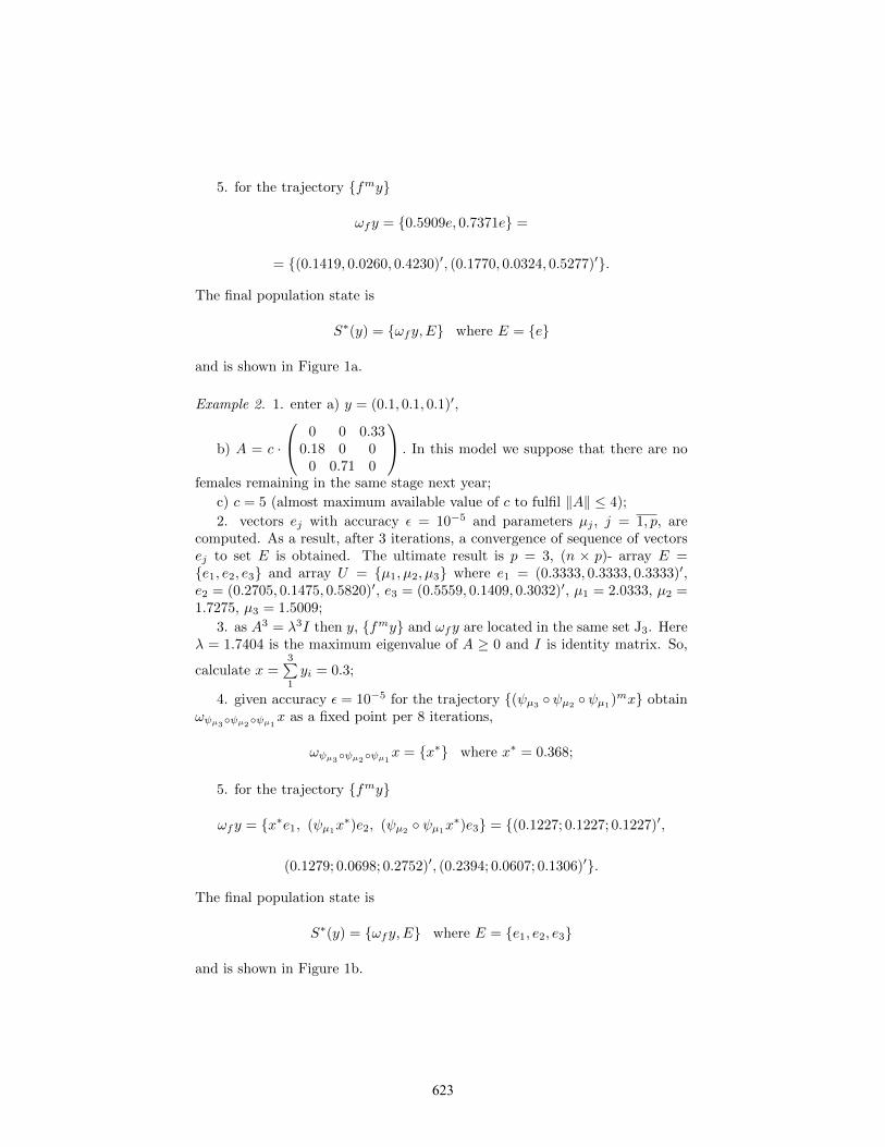
5. for the trajectory fmy

ωfy = 0.5909e, 0.7371e =

= (0.1419, 0.0260, 0.4230)′, (0.1770, 0.0324, 0.5277)′.

The final population state is

S∗(y) = ωfy,E where E = e

and is shown in Figure 1a.

Example 2. 1. enter a) y = (0.1, 0.1, 0.1)′,

b) A = c ·

0 0 0.330.18 0 0

0 0.71 0

. In this model we suppose that there are no

females remaining in the same stage next year;

c) c = 5 (almost maximum available value of c to fulfil ‖A‖ ≤ 4);

2. vectors ej with accuracy ε = 10−5 and parameters µj , j = 1, p, arecomputed. As a result, after 3 iterations, a convergence of sequence of vectorsej to set E is obtained. The ultimate result is p = 3, (n × p)- array E =e1, e2, e3 and array U = µ1, µ2, µ3 where e1 = (0.3333, 0.3333, 0.3333)′,e2 = (0.2705, 0.1475, 0.5820)′, e3 = (0.5559, 0.1409, 0.3032)′, µ1 = 2.0333, µ2 =1.7275, µ3 = 1.5009;

3. as A3 = λ3I then y, fmy and ωfy are located in the same set J3. Hereλ = 1.7404 is the maximum eigenvalue of A ≥ 0 and I is identity matrix. So,

calculate x =3∑1yi = 0.3;

4. given accuracy ε = 10−5 for the trajectory (ψµ3ψµ2

ψµ1)mx obtain

ωψµ3ψµ2ψµ1x as a fixed point per 8 iterations,

ωψµ3ψµ2ψµ1x = x∗ where x∗ = 0.368;

5. for the trajectory fmy

ωfy = x∗e1, (ψµ1x∗)e2, (ψµ2 ψµ1x

∗)e3 = (0.1227; 0.1227; 0.1227)′,

(0.1279; 0.0698; 0.2752)′, (0.2394; 0.0607; 0.1306)′.

The final population state is

S∗(y) = ωfy,E where E = e1, e2, e3

and is shown in Figure 1b.

623

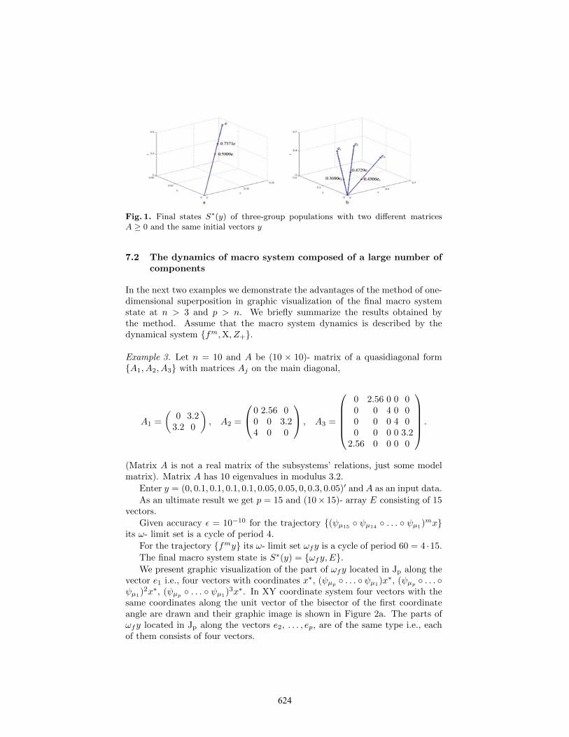
Fig. 1. Final states S∗(y) of three-group populations with two different matricesA ≥ 0 and the same initial vectors y

7.2 The dynamics of macro system composed of a large number ofcomponents

In the next two examples we demonstrate the advantages of the method of one-dimensional superposition in graphic visualization of the final macro systemstate at n > 3 and p > n. We briefly summarize the results obtained bythe method. Assume that the macro system dynamics is described by thedynamical system fm,X, Z+.

Example 3. Let n = 10 and A be (10 × 10)- matrix of a quasidiagonal formA1, A2, A3 with matrices Aj on the main diagonal,

A1 =

(0 3.2

3.2 0

), A2 =

0 2.56 00 0 3.24 0 0

, A3 =

0 2.56 0 0 00 0 4 0 00 0 0 4 00 0 0 0 3.2

2.56 0 0 0 0

.

(Matrix A is not a real matrix of the subsystems’ relations, just some modelmatrix). Matrix A has 10 eigenvalues in modulus 3.2.

Enter y = (0, 0.1, 0.1, 0.1, 0.1, 0.05, 0.05, 0, 0.3, 0.05)′ and A as an input data.

As an ultimate result we get p = 15 and (10× 15)- array E consisting of 15vectors.

Given accuracy ε = 10−10 for the trajectory (ψµ15 ψµ14

. . . ψµ1)mx

its ω- limit set is a cycle of period 4.

For the trajectory fmy its ω- limit set ωfy is a cycle of period 60 = 4 ·15.

The final macro system state is S∗(y) = ωfy,E.We present graphic visualization of the part of ωfy located in Jp along the

vector e1 i.e., four vectors with coordinates x∗, (ψµp . . . ψµ1)x∗, (ψµp . . .

ψµ1)2x∗, (ψµp . . . ψµ1

)3x∗. In XY coordinate system four vectors with thesame coordinates along the unit vector of the bisector of the first coordinateangle are drawn and their graphic image is shown in Figure 2a. The parts ofωfy located in Jp along the vectors e2, . . . , ep, are of the same type i.e., eachof them consists of four vectors.

624

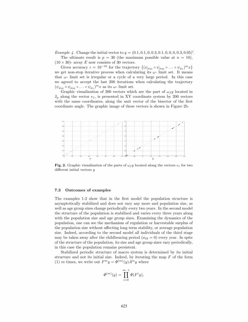
Example 4. Change the initial vector to y = (0.1, 0.1, 0, 0.3, 0.1, 0, 0, 0, 0.3, 0.05)′.The ultimate result is p = 30 (the maximum possible value at n = 10),

(10× 30)- array E now consists of 30 vectors.Given accuracy ε = 10−10 for the trajectory (ψµ30 ψµ29 . . . ψµ1)mx

we get non-stop iterative process when calculating its ω- limit set. It meansthat ω- limit set is irregular or a cycle of a very large period. In this casewe agreed to accept the last 200 iterations when calculating the trajectory(ψµ30

ψµ29 . . . ψµ1

)mx as its ω- limit set.Graphic visualization of 200 vectors which are the part of ωfy located in

Jp along the vector e1, is presented in XY coordinate system by 200 vectorswith the same coordinates, along the unit vector of the bisector of the firstcoordinate angle. The graphic image of these vectors is shown in Figure 2b.

Fig. 2. Graphic visualization of the parts of ωfy located along the vectors e1 for twodifferent initial vectors y

7.3 Outcomes of examples

The examples 1-2 show that in the first model the population structure isasymptotically stabilized and does not vary any more and population size, aswell as age group sizes change periodically every two years. In the second modelthe structure of the population is stabilized and varies every three years alongwith the population size and age group sizes. Examining the dynamics of thepopulation, one can see the mechanism of regulation or harvestable surplus ofthe population size without affecting long term stability, or average populationsize. Indeed, according to the second model all individuals of the third stagemay be taken away after the childbearing period (a33 = 0) every year. In spiteof the structure of the population, its size and age group sizes vary periodically,in this case the population remains persistent.

Stabilized periodic structure of macro system is determined by its initialstructure and not its initial size. Indeed, by iterating the map F of the form(1) m times, we write out Fmy = Φ(m)(y)Amy where

Φ(m)(y) =

m−1∏i=0

Φ(F iy),

625

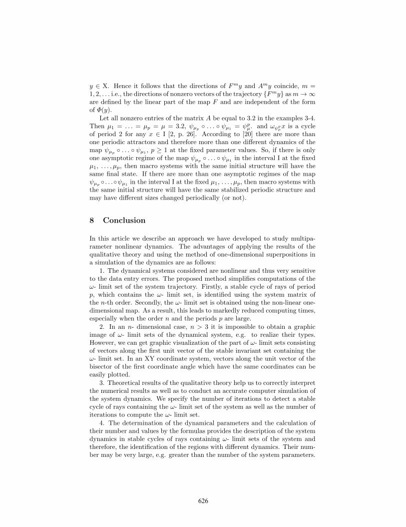
y ∈ X. Hence it follows that the directions of Fmy and Amy coincide, m =1, 2, . . . i.e., the directions of nonzero vectors of the trajectory Fmy asm→∞are defined by the linear part of the map F and are independent of the formof Φ(y).

Let all nonzero entries of the matrix A be equal to 3.2 in the examples 3-4.Then µ1 = . . . = µp = µ = 3.2, ψµp . . . ψµ1

= ψpµ. and ωψpµx is a cycleof period 2 for any x ∈ I [2, p. 26]. According to [20] there are more thanone periodic attractors and therefore more than one different dynamics of themap ψµp . . . ψµ1

, p ≥ 1 at the fixed parameter values. So, if there is onlyone asymptotic regime of the map ψµp . . . ψµ1

in the interval I at the fixedµ1, . . . , µp, then macro systems with the same initial structure will have thesame final state. If there are more than one asymptotic regimes of the mapψµp . . .ψµ1 in the interval I at the fixed µ1, . . . , µp, then macro systems withthe same initial structure will have the same stabilized periodic structure andmay have different sizes changed periodically (or not).

8 Conclusion

In this article we describe an approach we have developed to study multipa-rameter nonlinear dynamics. The advantages of applying the results of thequalitative theory and using the method of one-dimensional superpositions ina simulation of the dynamics are as follows:

1. The dynamical systems considered are nonlinear and thus very sensitiveto the data entry errors. The proposed method simplifies computations of theω- limit set of the system trajectory. Firstly, a stable cycle of rays of periodp, which contains the ω- limit set, is identified using the system matrix ofthe n-th order. Secondly, the ω- limit set is obtained using the non-linear one-dimensional map. As a result, this leads to markedly reduced computing times,especially when the order n and the periods p are large.

2. In an n- dimensional case, n > 3 it is impossible to obtain a graphicimage of ω- limit sets of the dynamical system, e.g. to realize their types.However, we can get graphic visualization of the part of ω- limit sets consistingof vectors along the first unit vector of the stable invariant set containing theω- limit set. In an XY coordinate system, vectors along the unit vector of thebisector of the first coordinate angle which have the same coordinates can beeasily plotted.

3. Theoretical results of the qualitative theory help us to correctly interpretthe numerical results as well as to conduct an accurate computer simulation ofthe system dynamics. We specify the number of iterations to detect a stablecycle of rays containing the ω- limit set of the system as well as the number ofiterations to compute the ω- limit set.

4. The determination of the dynamical parameters and the calculation oftheir number and values by the formulas provides the description of the systemdynamics in stable cycles of rays containing ω- limit sets of the system andtherefore, the identification of the regions with different dynamics. Their num-ber may be very large, e.g. greater than the number of the system parameters.

626

However, one can see that this number cannot be reduced without the loss ofaccuracy of the system behavior description.

Acknowledgements

The work is supported by the grant 0292/GF3 of Ministry of Education andScience of the Republic of Kazakhstan.

References

1. A.N. Sharkovskii. Co-existence of cycles of a continuous mapping of the line intoitself. Ukrainian Math J, 16:61-71, 1964.

2. A.N. Sharkovskii, Yu.L. Maistrenko, E.Yu. Romanenko. Difference Equations andTheir Applications, Naukova Dumka, Kiev, 1986 (in Russian).

3. M. Feigenbaum. Quantative universality for a class of nonlinear transfomaions. JStat Phys, 19:25-52, 1978.

4. R.M. May. Simple mathematical models with very complicated dynamics. Nature,261(5560):459-467, 1976.

5. A.G. Radwan. On some generalized discrete logistic maps. J Adv Res, vol. 4, issue2, 163-171, 2013.

6. G. Tiozzo. Topological entropy of quadratic polynomials and dimension of sec-tions of the Mandelbrot set. Adv in Math, vol. 273, no. 19, 651715, 2015.doi:10.1016/j.aim.2014.12.033

7. M. Joglekar and J.A Yorke. Robustness of periodic orbits in the presence of noise.Nonlinearity, vol. 28, no. 3, 697-711, 2015. doi:10.1088/0951-7715/28/3/697

8. Z. Arai, W. Kalies, H. Cocubu, K. Mischaikow et al. A Database Schema for theAnalysis of Global Dynamics of Multiparameter Systems. SIAM J Appl Dyn Syst,vol. 8, no. 3, 757-789, 2009.

9. I. Gohberg, P. Lancaster, L. Rodman. Invariant Subspaces of Matrices with Appli-cations, Siam, 2006.

10. A. Kaw, E. Kalu, D. Nguyen. Numerical methods with applications, Univ of SouthFlorida, 2009.

11. J. Sabuco, M.A.F. Sanjuan, and J.A. Yorke. Dynamics of partial control. Chaos,vol. 22, no. 4, 047507-1-047507-9, 2012.

12. A.S. de Paula, M.A. Savi. State space reconstruction applied to a multiparame-ter chaos control method. Meccanica, 50:207-216,2015. doi: 10.1007/s11012-014-0066-z

13. I.N. Pankratova, Cyclic Invariant Sets for One Class of Maps. Siberian Math J,vol. 50, no. 1, 107-116, 2009. doi:10.1007/s11202-009-0013-8

14. R. Muradore, R. Foroncelli and P. Fiorini. Statistical methods for estimatingthe dynamical parameters of manipulators. In: Proc. of joint 48th IEEE Confon Decision and Control and 28th Chinese Control Conf, 6472-6477, 2009. doi:10.1109/CDC.2009.5400194

15. I.N. Pankratova. Limit sets of manydimensional analogy of nonlinear logistic dif-ference equation. Differ Equ, vol. 32, no. 7, 1006-1008, 1996.

16. P.H. Leslie. The use of matrices in certain population mathematics. Biometrika,33:183-212, 1945.

17. D. O. Logofet. Projection matrices revisited: a potential-growth indicator and themerit of indication. J Math Sci, vol. 193, no. 5, 671-686, 2013.

627

18. I.N. Pankratova. On some properties of invariant subspaces of linear op-erator containing cycles of rays. In: Conf Program and Book of Ab-str of Conf MAT TRIAD, Herceg Novi, Montenegro, 49-50, 2013.http://mattriad2013.pmf.uns.ac.rs/programme.php

19. R. Lamberson, R. McKelvey, B. Noon, C. Voss. A Dynamic Analysis of NorthernSpotted Owl Viability in a Fragmented Forest Landscape. Conserv Biol, vol. 6,no. 4, 505-512, 1992.

20. J. Guckenhemer, G.F. Oster and A. Ipartchi. The Dynamics of Density DependentPopulation Models. J Math Biol, 4:101-147, 1976.

628

_________________

8th

CHAOS Conference Proceedings, 26-29 May 2015, Henri Poincaré Institute, Paris France

© 2015 ISAST

The Complete Bifurcation Analysis of Switching

Power Converters with Switching Delays

Dmitrijs Pikulins1

1 Institute of Radioelectronics, Riga Technical University, Riga, Latvia

(E-mail: dmitrijs.pikulins@rtu.lv)

Abstract. The nonlinear dynamics of switching power converters has been actively stud-

ied during several last decades, proving the existence of extremely complex dynamical

scenarios and uncommon routes to chaos in this kind of circuits. The main assumption in

the majority of researches was that the control circuitry consisted of ideal elements, dis-

carding all parasitics of feedback circuitry components. However, recently it has been

shown that the inherently arising nonidealities, such as delays, could lead to the drastic

changes in the overall dynamics of the system. This research is dedicated to the investi-

gation of the effects of the delays on the global nonlinear behavior of switching DC-DC

converters on the basis of complete bifurcation analysis, providing the most comprehen-

sive information on the causes and consequences of all nonlinear phenomena in the sys-

tems under study.

Keywords: Bifurcations, chaos, non-smooth phenomena, switching power converters

Introduction

Active research performed during several last decades showed that the com-

monly used linearized models, describing the dynamics of switching power con-

verters (SPC) are not capable of predicting the majority of instabilities, occur-

ring in those systems [1,2]. Thus the classical models fail to provide reliable in-

formation for the feedback designers that would allow the development of stable

control loops. The limited applicability of mentioned models has led to the de-

velopment of some alternative approaches, based on non-linear models and

analysis methodologies. While making the study of global dynamics of these

systems more complicated, the latter approaches allow increasing the robustness

and reliability of designed systems as the great amount of new unstable and po-

tentially dangerous regimes could be detected.

The vast majority of researchers, working on the analysis of non-linear

dynamics of SPC, have focused on the development of simplified models that

could be used within their investigations. However, it has been shown that

ignoring some unavoidable non-idealities of the control circuitry may lead to

erroneous results and misinterpretation of analytically obtained data [3]. One of

the most noticeable effects, that should be taken into account during the analysis

629

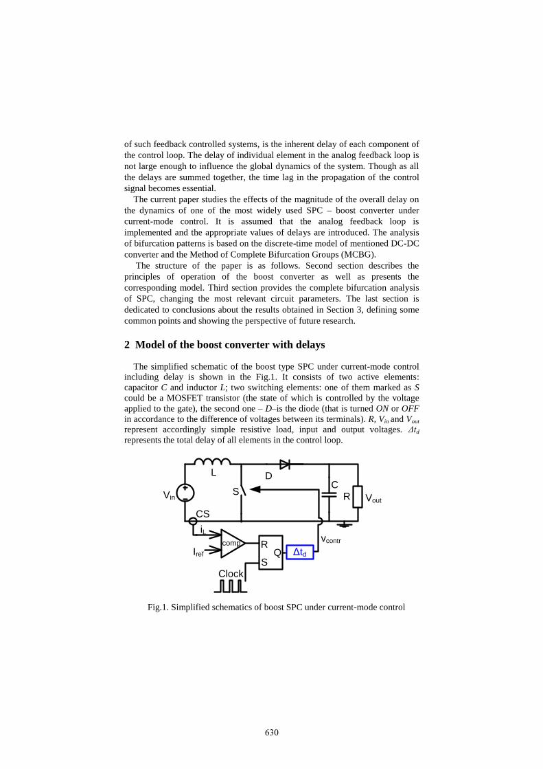
of such feedback controlled systems, is the inherent delay of each component of

the control loop. The delay of individual element in the analog feedback loop is

not large enough to influence the global dynamics of the system. Though as all

the delays are summed together, the time lag in the propagation of the control

signal becomes essential.

The current paper studies the effects of the magnitude of the overall delay on

the dynamics of one of the most widely used SPC – boost converter under

current-mode control. It is assumed that the analog feedback loop is

implemented and the appropriate values of delays are introduced. The analysis

of bifurcation patterns is based on the discrete-time model of mentioned DC-DC

converter and the Method of Complete Bifurcation Groups (MCBG).

The structure of the paper is as follows. Second section describes the

principles of operation of the boost converter as well as presents the

corresponding model. Third section provides the complete bifurcation analysis

of SPC, changing the most relevant circuit parameters. The last section is

dedicated to conclusions about the results obtained in Section 3, defining some

common points and showing the perspective of future research.

2 Model of the boost converter with delays

The simplified schematic of the boost type SPC under current-mode control

including delay is shown in the Fig.1. It consists of two active elements:

capacitor C and inductor L; two switching elements: one of them marked as S

could be a MOSFET transistor (the state of which is controlled by the voltage

applied to the gate), the second one – D–is the diode (that is turned ON or OFF

in accordance to the difference of voltages between its terminals). R, Vin and Vout

represent accordingly simple resistive load, input and output voltages. Δtd

represents the total delay of all elements in the control loop.

D

SVin

L

CR

Iref

Clock

QR

S

iLcomp

vcontr

Δtd

CS

Vout

Fig.1. Simplified schematics of boost SPC under current-mode control

630

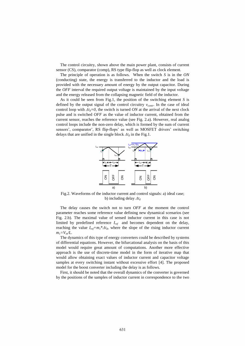
The control circuitry, shown above the main power plant, consists of current

sensor (CS), comparator (comp), RS type flip-flop as well as clock element.

The principle of operation is as follows. When the switch S is in the ON

(conducting) state, the energy is transferred to the inductor and the load is

provided with the necessary amount of energy by the output capacitor. During

the OFF interval the required output voltage is maintained by the input voltage

and the energy released from the collapsing magnetic field of the inductor.

As it could be seen from Fig.1, the position of the switching element S is

defined by the output signal of the control circuitry vcontr. In the case of ideal

control loop with Δtd=0, the switch is turned ON at the arrival of the next clock

pulse and is switched OFF as the value of inductor current, obtained from the

current sensor, reaches the reference value (see Fig. 2.a). However, real analog

control loops include the non-zero delay, which is formed by the sum of current

sensors’, comparator’, RS flip-flops’ as well as MOSFET drivers’ switching

delays that are unified in the single block Δtd in the Fig.1.

T

ON

OF

F

b)

in+1in

ton toff

Iref

Δtd

ON

T

ON

OF

F

a)

in+1

in

ton toff

Iref

ON

Iref+m1*Δtd

Fig.2. Waveforms of the inductor current and control signals: a) ideal case;

b) including delay Δtd

The delay causes the switch not to turn OFF at the moment the control

parameter reaches some reference value defining new dynamical scenarios (see

Fig. 2.b). The maximal value of sensed inductor current in this case is not

limited by predefined reference Iref and becomes dependent on the delay,

reaching the value Iref+m1*Δtd, where the slope of the rising inductor current

m1=Vin/L.

The dynamics of this type of energy converters could be described by systems

of differential equations. However, the bifurcational analysis on the basis of this

model would require great amount of computations. Another more effective

approach is the use of discrete-time model in the form of iterative map that

would allow obtaining exact values of inductor current and capacitor voltage

samples at every switching instant without excessive effort [4]. The proposed

model for the boost converter including the delay is as follows.

First, it should be noted that the overall dynamics of the converter is governed

by the positions of the samples of inductor current in correspondence to the two

631

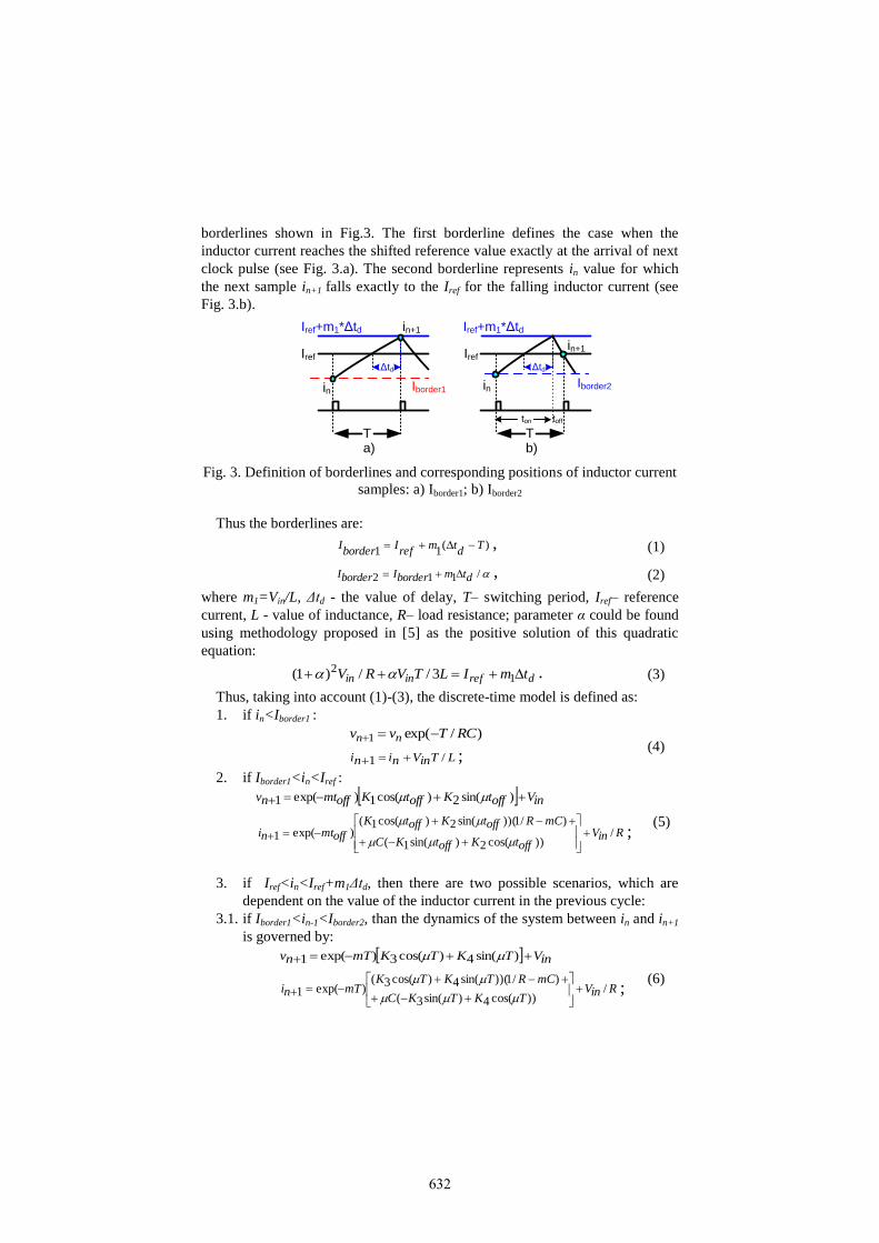
borderlines shown in Fig.3. The first borderline defines the case when the

inductor current reaches the shifted reference value exactly at the arrival of next

clock pulse (see Fig. 3.a). The second borderline represents in value for which

the next sample in+1 falls exactly to the Iref for the falling inductor current (see

Fig. 3.b).

T

in+1

in

Iref

Δtd

Iref+m1*Δtd

T

in+1

in

ton toff

Iref

Iref+m1*Δtd

Δtd

Iborder1Iborder2

a) b)

Fig. 3. Definition of borderlines and corresponding positions of inductor current

samples: a) Iborder1; b) Iborder2

Thus the borderlines are:

)(11

Td

tmref

Iborder

I , (1)

/112 dtmborderIborderI , (2)

where m1=Vin/L, Δtd - the value of delay, T– switching period, Iref– reference

current, L - value of inductance, R– load resistance; parameter α could be found

using methodology proposed in [5] as the positive solution of this quadratic

equation:

drefinin tmILTVRV 12 3//)1( . (3)

Thus, taking into account (1)-(3), the discrete-time model is defined as:

1. if in<Iborder1 :

)/exp(1 RCTvv nn

LTinVnini /1 ; (4)

2. if Iborder1<in<Iref :

inVofftKofftKoffmtnv )sin(2)cos(1)exp(1

RinV

offtKofftKC

mCRofftKofftK

offmtni /))cos(2)sin(1(

)/1))(sin(2)cos(1()exp(1

;

(5)

3. if Iref<in<Iref+m1Δtd, then there are two possible scenarios, which are

dependent on the value of the inductor current in the previous cycle:

3.1. if Iborder1<in-1<Iborder2, than the dynamics of the system between in and in+1

is governed by:

inVTKTKmTnv )sin(4)cos(3)exp(1

RinV

TKTKC

mCRTKTKmTni /

))cos(4)sin(3(

)/1))(sin(4)cos(3()exp(1

;

(6)

632

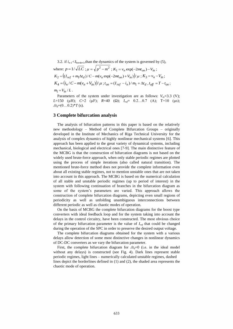
3.2. if in-1<Iborder1,than the dynamics of the system is governed by (5),

where: LCp /1 ; 22 mp ; inonn VmtvK )2exp(1 ;

/))2exp((/)( 12 inonndref VmtvmCtmIK ; inn VvK 3 ;

/)(/4 innn VvmCiK ; dnrefon tmiIt 1/)( , onoff tTt ;

LVm in /1 .

Parameters of the system under investigation are as follows: Vin=3.3 (V);

L=150 (µH); C=2 (µF); R=40 (Ω); Iref= 0.2…0.7 (A); T=10 (µs);

Δtd=(0…0.2)*T (s).

3 Complete bifurcation analysis

The analysis of bifurcation patterns in this paper is based on the relatively

new methodology – Method of Complete Bifurcation Groups – originally

developed in the Institute of Mechanics of Riga Technical University for the

analysis of complex dynamics of highly nonlinear mechanical systems [6]. This

approach has been applied to the great variety of dynamical systems, including

mechanical, biological and electrical ones [7-9]. The main distinctive feature of

the MCBG is that the construction of bifurcation diagrams is not based on the

widely used brute-force approach, when only stable periodic regimes are plotted

using the process of simple iterations (also called natural transition). The

mentioned brute-force method does not provide the complete information even

about all existing stable regimes, not to mention unstable ones that are not taken

into account in this approach. The MCBG is based on the numerical calculation

of all stable and unstable periodic regimes (up to period of interest) in the

system with following continuation of branches in the bifurcation diagram as

some of the system’s parameters are varied. This approach allows the

construction of complete bifurcation diagrams, depicting even small regions of

periodicity as well as unfolding unambiguous interconnections between

different periodic as well as chaotic modes of operation.

On the basis of MCBG the complete bifurcation diagrams for the boost type

converters with ideal feedback loop and for the system taking into account the

delays in the control circuitry, have been constructed. The most obvious choice

of the primary bifurcation parameter is the value of Iref that could be changed

during the operation of the SPC in order to preserve the desired output voltage.

The complete bifurcation diagrams obtained for the system with a various

delays allow detection of some most distinctive changes in nonlinear dynamics

of DC-DC converters as we vary the bifurcation parameter.

First, the complete bifurcation diagram for Δtd=0 (i.e. in the ideal model

without any delays) is constructed (see Fig. 4). Dark lines represent stable

periodic regimes, light lines – numerically calculated unstable regimes, dashed

lines depict the borderlines defined in (1) and (2), the shaded area represents the

chaotic mode of operation.

633

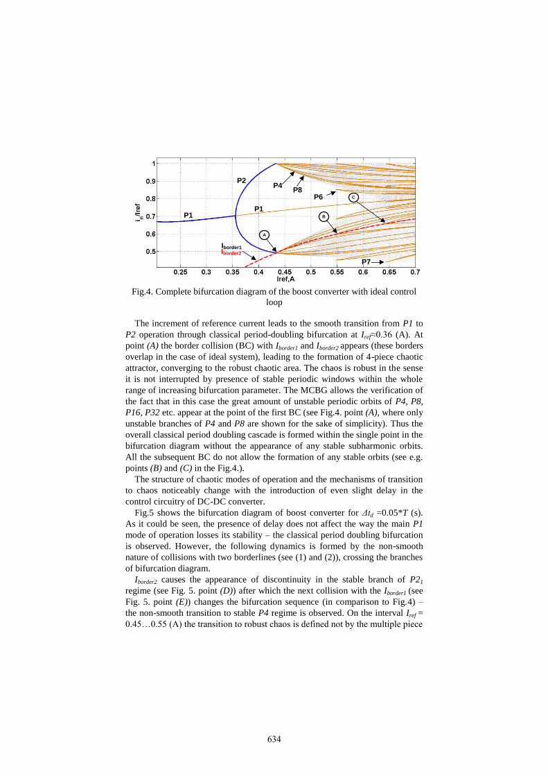
P1P1

P2P4

P8

Iborder1Iborder2

P6

P7

A

B

C

Fig.4. Complete bifurcation diagram of the boost converter with ideal control

loop

The increment of reference current leads to the smooth transition from P1 to

P2 operation through classical period-doubling bifurcation at Iref≈0.36 (A). At

point (A) the border collision (BC) with Iborder1 and Iborder2 appears (these borders

overlap in the case of ideal system), leading to the formation of 4-piece chaotic

attractor, converging to the robust chaotic area. The chaos is robust in the sense

it is not interrupted by presence of stable periodic windows within the whole

range of increasing bifurcation parameter. The MCBG allows the verification of

the fact that in this case the great amount of unstable periodic orbits of P4, P8,

P16, P32 etc. appear at the point of the first BC (see Fig.4. point (A), where only

unstable branches of P4 and P8 are shown for the sake of simplicity). Thus the

overall classical period doubling cascade is formed within the single point in the

bifurcation diagram without the appearance of any stable subharmonic orbits.

All the subsequent BC do not allow the formation of any stable orbits (see e.g.

points (B) and (C) in the Fig.4.).

The structure of chaotic modes of operation and the mechanisms of transition

to chaos noticeably change with the introduction of even slight delay in the

control circuitry of DC-DC converter.

Fig.5 shows the bifurcation diagram of boost converter for Δtd =0.05*T (s).

As it could be seen, the presence of delay does not affect the way the main P1

mode of operation losses its stability – the classical period doubling bifurcation

is observed. However, the following dynamics is formed by the non-smooth

nature of collisions with two borderlines (see (1) and (2)), crossing the branches

of bifurcation diagram.

Iborder2 causes the appearance of discontinuity in the stable branch of P21

regime (see Fig. 5. point (D)) after which the next collision with the Iborder1 (see

Fig. 5. point (E)) changes the bifurcation sequence (in comparison to Fig.4) –

the non-smooth transition to stable P4 regime is observed. On the interval Iref =

0.45…0.55 (A) the transition to robust chaos is defined not by the multiple piece

634

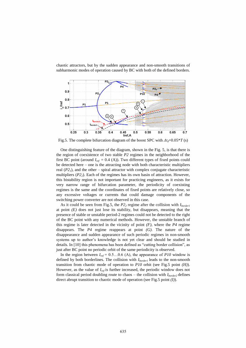
chaotic attractors, but by the sudden appearance and non-smooth transitions of

subharmonic modes of operation caused by BC with both of the defined borders.

P1P1

P4

P21

Iborder1

Iborder2

P10

P22

P4

P22

D E

F

G

H

I

Fig.5. The complete bifurcation diagram of the boost SPC with Δtd=0.05*T (s)

One distinguishing feature of the diagram, shown in the Fig. 5, is that there is

the region of coexistence of two stable P2 regimes in the neighborhood of the

first BC point (around Iref = 0.4 (A)). Two different types of fixed points could

be detected here – one is the attracting node with both characteristic multipliers

real (P21), and the other – spiral attractor with complex conjugate characteristic

multipliers (P22). Each of the regimes has its own basin of attraction. However,

this bistability region is not important for practicing engineers, as it exists for

very narrow range of bifurcation parameter, the periodicity of coexisting

regimes is the same and the coordinates of fixed points are relatively close, so

any excessive voltages or currents that could damage components of the

switching power converter are not observed in this case.

As it could be seen from Fig.5, the P22 regime after the collision with Iborder1

at point (E) does not just lose its stability, but disappears, meaning that the

presence of stable or unstable period-2 regimes could not be detected to the right

of the BC point with any numerical methods. However, the unstable branch of

this regime is later detected in the vicinity of point (F), where the P4 regime

disappears. The P4 regime reappears at point (G). The nature of the

disappearance and sudden appearance of such periodic regimes in non-smooth

systems up to author’s knowledge is not yet clear and should be studied in

details. In [10] this phenomena has been defined as “cutting border collision”, as

just after BC point no periodic orbit of the same periodicity is observed.

In the region between Iref = 0.5…0.6 (A), the appearance of P10 window is

defined by both borderlines. The collision with Iborder1 leads to the non-smooth

transition from chaotic mode of operation to P10 orbit (see Fig.5 point (H)).

However, as the value of Iref is further increased, the periodic window does not

form classical period doubling route to chaos – the collision with Iborder2 defines

direct abrupt transition to chaotic mode of operation (see Fig.5 point (I)).

635

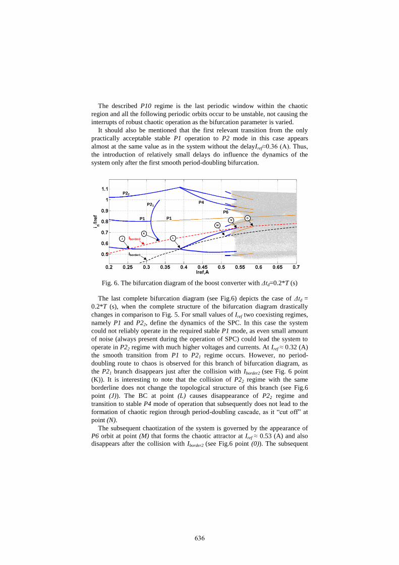
The described P10 regime is the last periodic window within the chaotic

region and all the following periodic orbits occur to be unstable, not causing the

interrupts of robust chaotic operation as the bifurcation parameter is varied.

It should also be mentioned that the first relevant transition from the only

practically acceptable stable P1 operation to P2 mode in this case appears

almost at the same value as in the system without the delayIref≈0.36 (A). Thus,

the introduction of relatively small delays do influence the dynamics of the

system only after the first smooth period-doubling bifurcation.

P1P1

P21

Iborder1

Iborder2

P22

P4

P6

M

K

J

NO

L

Fig. 6. The bifurcation diagram of the boost converter with Δtd=0.2*T (s)

The last complete bifurcation diagram (see Fig.6) depicts the case of Δtd =

0.2*T (s), when the complete structure of the bifurcation diagram drastically

changes in comparison to Fig. 5. For small values of Iref two coexisting regimes,

namely P1 and P22, define the dynamics of the SPC. In this case the system

could not reliably operate in the required stable P1 mode, as even small amount

of noise (always present during the operation of SPC) could lead the system to

operate in P22 regime with much higher voltages and currents. At Iref ≈ 0.32 (A)

the smooth transition from P1 to P21 regime occurs. However, no period-

doubling route to chaos is observed for this branch of bifurcation diagram, as

the P21 branch disappears just after the collision with Iborder2 (see Fig. 6 point

(K)). It is interesting to note that the collision of P22 regime with the same

borderline does not change the topological structure of this branch (see Fig.6

point (J)). The BC at point (L) causes disappearance of P22 regime and

transition to stable P4 mode of operation that subsequently does not lead to the

formation of chaotic region through period-doubling cascade, as it “cut off” at

point (N).

The subsequent chaotization of the system is governed by the appearance of

P6 orbit at point (M) that forms the chaotic attractor at Iref ≈ 0.53 (A) and also

disappears after the collision with Iborder2 (see Fig.6 point (0)). The subsequent

636

chaotic region is robust, as the two borderlines do not allow the formation of

stable periodic orbits or coexisting attractors.

4 Conclusions

This paper showed that the discrete-time model of the boost type SPC under

current-mode control could be effectively improved, including the value of total

delay in the control loop. The results of complete bifurcation analysis confirm

that even small values of delay may drastically change the structure of

bifurcation diagrams, causing the appearance of highly non-smooth events and

uncommon routes to chaos. The most distinctive phenomena include the

appearance of coexisting attractors even in the region of P1 operation, as well as

sudden disappearance and reappearance of stable and unstable periodic regimes

after border collisions. The obtained results prove that it is not possible to

provide reliable prediction of operating modes and their stability of SPC without

taking into account time lag effects. It should be noted, that relatively small

values of delays (up to 20% of switching period) were chosen, considering the

analog control loops. However the typical values of delays in digital control

circuitry could be much greater and the effects of these delays on the global

dynamics of SPC will be addressed in the future research.

Acknowledgements This research was funded by a grant (No. 467/2012) from the Latvian Council

of Science.

References

1. E. R. Vilamitjana, E. Alarcon, A. El Aroudi. Chaos in switching converters for

power management. New York: Springer, 2012.

2. C. K. Tse, M. Li. Design-oriented bifurcation analysis of power electronics

systems, Int. Journal of Bifurcations and Chaos, vol. 21, no. 6, pp. 1523–1537,

2011.

3. S. Banerjee, S. Parui, A. Gupta. Dynamical effects of missed switching in current

mode controlled dc-dc converter, IEEE Trans. on circuits and systems, vol. 51, no.

12, pp. 649–655, 2004.

4. D.C. Hammil, J.H.B. Deane, D.J. Jefferies. Modeling of chaotic dc/dc converters by

iterative nonlinear mappings. IEEE Transactions on Circuits and Systems Part I,

vol.35, no.8, 25-36, 1992.

5. S. Banerjee and G. C. Verghese (Ed.) . Nonlinear Phenomena in Power Electronics.

Attractors, Bifurcations, Chaos, and Nonlinear Control, IEEE Press, 2001.

6. M. Zakrzhevsky, “Bifurcation theory of nonlinear dynamics and chaos. Periodic

skeletons and rare attractors”, Proc. 2 nd Int. Symposium (RA 2011), pp. 26–30,

2011.

7. M.V. Zakrzhevsky and D. A. Pikulin (Eds.). Rare Attractors in Discrete Nonlinear

Dynamical Systems, Riga, Latvia, 2013.

637

8. D. Pikulins. Complete Bifurcation Analysis of DC-DC Converters Under Current

Mode Control, Journal of Physics: Conference Series „Physics and Mathematics of

Nonlinear Phenomena 2013”, Issue 1, Vol. 482, 2014.

9. D. Pikulins. Exploring Types of Instabilities in Switching Power Converters: the

Complete Bifurcation Analysis, Electronics and Electrical Engineering, Kaunas,

Lithiuania, Technologija, -No.5, pp. 76-79, 2014.

10. D. Pikulins. The Mechanisms of Chaotization in Switching Power Converters with

Compensation Ramp. CHAOS 2014 Proceedings 7th Chaotic Modeling and

Simulation International Conference , Portugal, Lisbon, 7-10 June, 2014. pp.367-

375.

638

Fractional Chen Chaotic Network

Carla M.A. Pinto1 and Ana R.M. Carvalho2

1 School of Engineering, Polytechnic of Porto, and Centre for Mathematics of the Universityof Porto, Rua Dr Antonio Bernardino de Almeida, 431, 4200-072 Porto, Portugal(E-mail: cap@isep.ipp.pt, corresponding author)

2 Faculty of Aciences, University of Porto, Rua do Campo Alegre s/n, 4169-002 Porto,Portugal(E-mail: up200802541@fc.up.pt)

Abstract. We analyze a fractional order model of a network of one ring of three cells coupledto a ‘buffer’ cell. By cell we mean a nonlinear system of ordinary differential equations. Thefull network has Z3 symmetry group. We consider the Chen chaotic oscillator to model cells’internal dynamics. We observe interesting dynamical patterns, such as steady-states, rotatingwaves and chaos, for distinct values of the parameter c of the Chen oscillator and the derivativeof fractional order α . The different patterns seem to appear through a sequence of Hopf andperiod-doubling bifurcations. Possible explanations for the peculiar patterns are the symmetryof the network and the dynamical characteristics of the Chen oscillator, used to model cells’internal dynamics.Keywords: fractional Chen oscillators, Z3 symmetry, chaos.

1 Introduction

The theory of networks of coupled cells has taken a major breakthrough in the lastfew years, mainly due to the work of Golubitsky, Stewart, and co-authors [3,5,4].These networks appear in many areas of science, from biology, economy, ecology,neuroscience, computation, and physics [11,1,14,6]. Particular attention has beengiven to patterns of synchrony [9], phase-locking modes, resonance, and quasiperi-odicity [1,10].

Networks of coupled cells are schematically identif ed with directed graphs, wherethe nodes (cells) represent dynamical systems, and the arrows indicate the couplingsbetween them.

In this paper, we study the dynamical features of the coupled cell systems as-sociated to the network in Figure 1, for variation of the fractional order derivativeα ∈ [0,1].

In Section 2, we summarize some concepts of the theory of coupled cell networksand bifurcation theory, for symmetric dynamical systems. In Section 3, we simulatethe coupled cell system associated with the network in Figure 1. In Section 4, we statethe main conclusions of the current work and sketch some future research.

8thCHAOS Conference Proceedings, 26-29 May 2015, Henri Poincare Institute, ParisFrance

c© 2015 ISAST

639

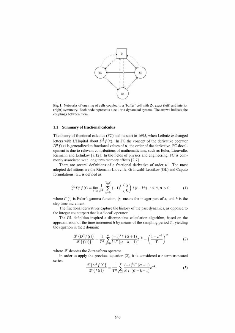
Fig. 1: Networks of one ring of cells coupled to a ‘buffer’ cell with Z3 exact (left) and interior(right) symmetry. Each node represents a cell or a dynamical system. The arrows indicate thecouplings between them.

1.1 Summary of fractional calculus

The theory of fractional calculus (FC) had its start in 1695, when Leibniz exchangedletters with L’Hopital about D

12 f (x). In FC the concept of the derivative operator

Dα f (x) is generalized to fractional values of α , the order of the derivative. FC devel-opment is due to relevant contributions of mathematicians, such as Euler, Liouvulle,Riemann and Letnikov [8,12]. In the f elds of physics and engineering, FC is com-monly associated with long term memory effects [2,7].

There are several def nitions of a fractional derivative of order α . The mostadopted def nitions are the Riemann-Liouville, Grunwald-Letnikov (GL) and Caputoformulations. GL is def ned as:

GLa Dα

t f (t) = limh→0

1hα

[ t−ah ]

∑k=0

(−1)k(

αk

)

f (t − kh) , t > a, α > 0 (1)

where Γ (·) is Euler’s gamma function, [x] means the integer part of x, and h is thestep time increment.

The fractional derivatives capture the history of the past dynamics, as opposed tothe integer counterpart that is a ‘local’ operator.

The GL def nition inspired a discrete-time calculation algorithm, based on theapproximation of the time increment h by means of the sampling period T , yieldingthe equation in the z domain:

Z Dα f (t)Z f (t)

=1

Tα

∞

∑k=0

(−1)kΓ (α + 1)k!Γ (α − k+ 1)

z−k =

(

1− z−1

T

)α

(2)

where Z denotes the Z-transform operator.In order to apply the previous equation (2), it is considered a r-term truncated

series:Z Dα f (t)Z f (t)

=1

Tα

r

∑k=0

(−1)kΓ (α + 1)k!Γ (α − k+ 1)

z−k (3)

640

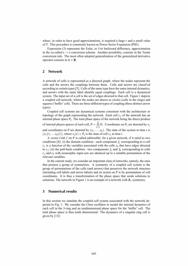
where, in order to have good approximations, is required a large r and a small valueof T . This procedure is commonly known as Power Series Expansion (PSE).

Expression (3) represents the Euler, or f rst backward difference, approximationin the so-called s→ z conversion scheme. Another possibility, consists in the Tustinconversion rule. The most often adopted generalization of the generalized derivativeoperator consists in α ∈ R.

2 Network

A network of cells is represented as a directed graph, where the nodes represent thecells and the arrows the couplings between them. Cells and arrows are classif edaccording to certain types [5]. Cells of the same type have the same internal dynamics,and arrows with the same label identify equal couplings. Each cell is a dynamicalsystem. The input set of a cell is the set of edges directed to that cell. Figure 1 depictsa coupled cell network, where the nodes are drawn as circles (cells in the rings) andsquares (‘buffer’ cell). There are three different types of coupling (three distinct arrowtypes).

Coupled cell systems are dynamical systems consistent with the architecture ortopology of the graph representing the network. Each cell c j of the network has aninternal phase space Pj . The total phase space of the network being the direct product

of internal phases spaces of each cell, P=n∏i=1

Pi . Coordinates on Pj are denoted by x j

and coordinates on P are denoted by (x1, . . . ,xn). The state of the system at time t is(x1(t), ...,xn(t)), where x j(t) ∈ Pj is the state of cell c j at time t.

A vector f eld f on P is called admissible, for a given network, if it satisf es twoconditions [4]: (i) the domain condition - each component f j corresponding to a cellc j is a function of the variables associated with the cells ck that have edges directedto c j ; (ii) the pull-back condition - two components f j and fk corresponding to cellsc j and ck with isomorphic input sets are identical up to a suitable permutation of therelevant variables.

In the current study, we consider an important class of networks, namely, the onesthat possess a group of symmetries. A symmetry of a coupled cell system is thegroup of permutations of the cells (and arrows) that preserves the network structure(including cell-labels and arrow-labels) and its action on P is by permutation of cellcoordinates. It is thus a transformation of the phase space that sends solutions tosolutions. The network in Figure 1 is an example of a network with Z3 symmetry.

3 Numerical results

In this section we simulate the coupled cell system associated with the network de-picted in Fig. 1. We consider the Chen oscillator to model the internal dynamics ofeach cell in the 3-ring and an unidimensional phase space for the ‘buffer’ cell. Thetotal phase space is thus tenth dimensional. The dynamics of a singular ring cell isgiven by [13]:

641

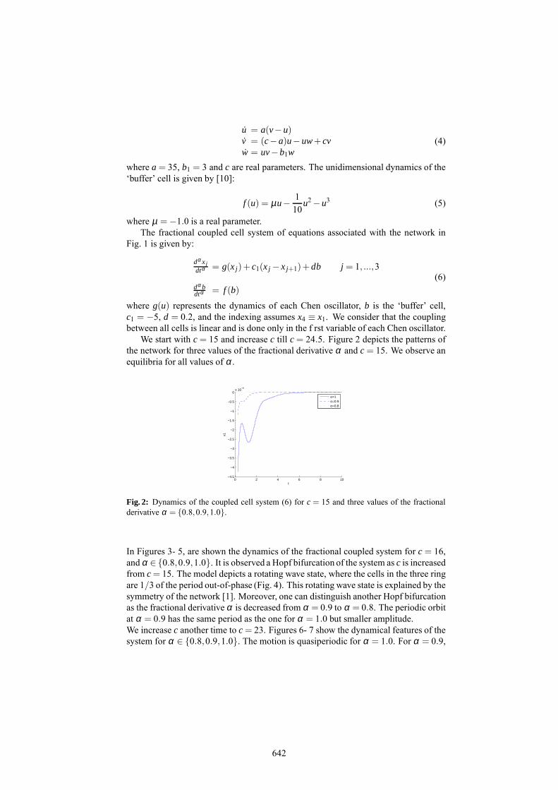
u = a(v−u)v = (c−a)u−uw+ cvw = uv−b1w

(4)

where a= 35, b1 = 3 and c are real parameters. The unidimensional dynamics of the‘buffer’ cell is given by [10]:

f (u) = µu−110

u2−u3 (5)

where µ =−1.0 is a real parameter.The fractional coupled cell system of equations associated with the network in

Fig. 1 is given by:

dα xjdtα = g(x j)+ c1(x j − x j+1)+db j = 1, ...,3

dα bdtα = f (b)

(6)

where g(u) represents the dynamics of each Chen oscillator, b is the ‘buffer’ cell,c1 = −5, d = 0.2, and the indexing assumes x4 ≡ x1. We consider that the couplingbetween all cells is linear and is done only in the f rst variable of each Chen oscillator.

We start with c= 15 and increase c till c= 24.5. Figure 2 depicts the patterns ofthe network for three values of the fractional derivative α and c= 15. We observe anequilibria for all values of α .

0 2 4 6 8 10−4.5

−4

−3.5

−3

−2.5

−2

−1.5

−1

−0.5

0x 10

−8

t

x1

α=1α=0.9α=0.8

Fig. 2: Dynamics of the coupled cell system (6) for c = 15 and three values of the fractionalderivative α = 0.8,0.9,1.0.

In Figures 3- 5, are shown the dynamics of the fractional coupled system for c= 16,andα ∈ 0.8,0.9,1.0. It is observed a Hopf bifurcation of the system as c is increasedfrom c= 15. The model depicts a rotating wave state, where the cells in the three ringare 1/3 of the period out-of-phase (Fig. 4). This rotating wave state is explained by thesymmetry of the network [1]. Moreover, one can distinguish another Hopf bifurcationas the fractional derivative α is decreased from α = 0.9 to α = 0.8. The periodic orbitat α = 0.9 has the same period as the one for α = 1.0 but smaller amplitude.We increase c another time to c= 23. Figures 6- 7 show the dynamical features of thesystem for α ∈ 0.8,0.9,1.0. The motion is quasiperiodic for α = 1.0. For α = 0.9,

642

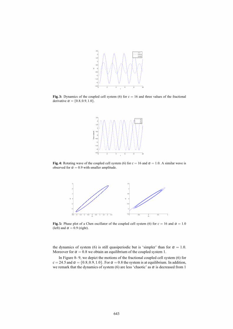
0 2 4 6 8 10−2.5

−2

−1.5

−1

−0.5

0

0.5

1

1.5

2

2.5

t

x1

α=1α=0.9α=0.8

Fig. 3: Dynamics of the coupled cell system (6) for c = 16 and three values of the fractionalderivative α = 0.8,0.9,1.0.

0 2 4 6 8 10−2.5

−2

−1.5

−1

−0.5

0

0.5

1

1.5

2

2.5

t

Che

n ne

twor

k

u1u2u3

Fig. 4: Rotating wave of the coupled cell system (6) for c= 16 and α = 1.0. A similar wave isobserved for α = 0.9 with smaller amplitude.

−2.5 −2 −1.5 −1 −0.5 0 0.5 1 1.5 2 2.5−3

−2

−1

0

1

2

3

x1

x2

−1 −0.5 0 0.5 1−1.5

−1

−0.5

0

0.5

1

1.5

x1

x2

Fig. 5: Phase plot of a Chen oscillator of the coupled cell system (6) for c = 16 and α = 1.0(left) and α = 0.9 (right).

the dynamics of system (6) is still quasiperiodic but is ‘simpler’ than for α = 1.0.Moreover for α = 0.8 we obtain an equilibrium of the coupled system 1.

In Figure 8- 9, we depict the motions of the fractional coupled cell system (6) forc= 24.5 and α = 0.8,0.9,1.0. For α = 0.8 the system is at equilibrium. In addition,we remark that the dynamics of system (6) are less ‘chaotic’ as α is decreased from 1

643

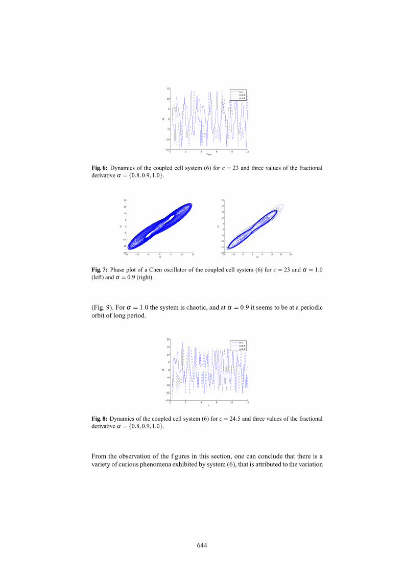
0 2 4 6 8 10−15

−10

−5

0

5

10

15

Time

x1

α=1α=0.9α=0.8

Fig. 6: Dynamics of the coupled cell system (6) for c = 23 and three values of the fractionalderivative α = 0.8,0.9,1.0.

−15 −10 −5 0 5 10 15−20

−15

−10

−5

0

5

10

15

20

x1

x2

−15 −10 −5 0 5 10 15 20−20

−15

−10

−5

0

5

10

15

20

25

x1

x2

Fig. 7: Phase plot of a Chen oscillator of the coupled cell system (6) for c = 23 and α = 1.0(left) and α = 0.9 (right).

(Fig. 9). For α = 1.0 the system is chaotic, and at α = 0.9 it seems to be at a periodicorbit of long period.

0 2 4 6 8 10−20

−15

−10

−5

0

5

10

15

20

t

x1

α=1α=0.9α=0.8

Fig. 8: Dynamics of the coupled cell system (6) for c= 24.5 and three values of the fractionalderivative α = 0.8,0.9,1.0.

From the observation of the f gures in this section, one can conclude that there is avariety of curious phenomena exhibited by system (6), that is attributed to the variation

644

−20 −15 −10 −5 0 5 10 15 20−25

−20

−15

−10

−5

0

5

10

15

20

25

x1

x2

−15 −10 −5 0 5 10 15 20−20

−15

−10

−5

0

5

10

15

20

x1

x2

Fig. 9: Phase plot of a Chen oscillator of the coupled cell system (6) for c= 24.5 and α = 1.0(left) and α = 0.9 (right).

of parameter c of the Chen oscillator, and is also due to the order of the fractionalderivative α . This will be further studied in future work.

4 Conclusions

We analyze curious patterns arising in a fractional order network of one ring of threecells coupled to a ‘buffer cell. We observe a broad range of dynamical features forincreasing c and as α is decreased from 1. The exotic behaviors are explained bythe symmetry of the network, the characteristics of the Chen oscillator, used to modelcells’ internal dynamics, and the fractional order derivative. Future work will focus onanalyzing theoretically the role of the derivative of fractional order α as a bifurcationparameter of the network.

Acknowledgments

The author was partially funded by the European Regional Development Fund throughthe programCOMPETE and by the PortugueseGovernment through the FCT - Fundacaopara a Ciencia e a Tecnologia under the project PEst-C/MAT/UI0144/2013. The re-search of Ana Carvalhowas supported by a FCT grant with reference SFRH/BD/96816/2013.

References

1. F. Antoneli, A.P.S. Dias and C.M.A. Pinto. Quasi-periodic states in coupled rings of cells.Communications in Nonlinear Science and Numerical Simulations, 15, 1048–1062, 2010.

2. D. Baleanu, K. Diethelm, E. Scalas, J.J. Trujillo. Fractional Calculus: Models and Numeri-cal Methods, Series on Complexity, Nonlinearity and Chaos, World Scientif c PublishingCompany, Singapore, 2012.

3. M. Golubitsky, M. Nicol and I. Stewart. Some curious phenomena in coupled cell systems.Journal of Nonlinear Science, 14, 207–236, 2004.

4. M. Golubitsky, I. Stewart. Nonlinear dynamics of networks: the groupoid formalism. BullAm Math Soc, 43, 305–364, 2006.

5. M. Golubitsky, I. Stewart, A. Torok. Patterns of synchrony in coupled cell networks withmultiple arrows. SIAM J Appl Dyn Syst4(1), 78–100, 2005.

645

6. X. Gong , D. Liu and B. Wang. Chaotic system synchronization with tridiagonal structureand its initial investigation in complex power systems. Journal of Vibration and Control,3(20), 447–457, 2014.

7. C.M. Ionescu. The human respiratory system: an analysis of the interplay between anatomy,structure, breathing and fractal dynamics, Series in BioEngineering, Springer-Verlag,London, 2013.

8. K.B. Oldham, J. Spanier, The fractional calculus: theory and application of differentiationand integration to arbitrary order, Academic Press, 1974.

9. A. Pikovsky, M. Rosenblum and J. Kurths. Synchronization, A Universal Concept in Nonlin-ear Sciences, Cambridge: Cambridge University Press, 2001.

10. C.M.A. Pinto and A.R.M. Carvalho. Strange patterns in one ring of Chen oscillators coupledto a ‘buffer’ cell. Journal of Vibration and Control, text, 1–29, published online 2014.

11. C.M.A. Pinto and M. Golubitsky. Central pattern generators for bipedal locomotion. Journalof Mathematical Biology, 53, 474–489, 2006.

12. S.G. Samko, A.A. Kilbas, O.I. Marichev, Fractional integrals and derivatives: theory andapplications.Gordon and Breach Science Publishers, 1993.

13. T. Ueta and G. Chen. Bifurcation analysis of Chen’s attractor. International Journal of Bi-furcation and Chaos, 10, 1917–1931, 2000.

14. J. Zhu, J. Lu and X. Yu. Flocking of multi-agent nonholonomic systems with proximitygraphs. IEEE Transactions on Circuits and Systems, 60(1), 199–210, 2013.

646

_________________

8th CHAOS Conference Proceedings, 26-29 May 2015, Henri Poincaré Institute, Paris France

© 2015 ISAST

Fractal Radar: Towards 1980 – 2015

Alexander A. Potapov

V.A.Kotel’nikov Institute of Radio Engineering and Electronics, Russian Academy of Sciences, 125009 Moscow, Russia

(E-mail: potapov@cplire.ru) Abstract. Results of application of theory of fractal and chaos, scaling effects and fractional operators in the fundamental issues of the radar and radio physical are presented in this report. The key point is detection and processing of super weak signals against the background of non-Gaussian intensive noises and strays. An alternative – the radar rang is increased dramatically. The results of researches of spectrum fractal dimensions of lightning discharge in the middle atmosphere at attitudes from 20 to 100 kilometres which are above the absolute of clouds are presented. The author has been investigating these issues 35 years equally and has obtained results of big scientific and practical worth. The reader is invited to look at the total of the title fundamental problems with the synergetic point of view of non-Markovian micro- and macro systems. Keywords: Fractal, Scaling, Texture, Chaos, Radar, Signals, Detectors, Fractal Radio-Systems, Ionosphere, Elves, Jets, Sprites. 1 Introduction

The entire current radio engineering is based on the classical theory of an integer measure and an integer calculation. Thus an extensive area of mathematical analysis which name is the fractional calculation and which deals with derivatives and integrals of a random (real or complex) order as well as the fractal theory has been historically turned out "outboard" (!). At the moment the integer measures (integrals and derivatives with integer order), Gaussian statistics, Markov processes etc. are mainly and habitually used everywhere in the radio physics, radio electronics and processing of multidimensional signals. It is worth noting that the Markov processes theory has already reached its satiation and researches are conducted at the level of abrupt complication of synthesized algorithms. Radar systems should be considered with relation to open dynamical systems. Improvement of classical radar detectors of signals and its mathematical support basically reached its saturation and limit. It forces to look for fundamentally new ways of solving of problem of increasing of sensitivity or range of coverage for various radio systems.

In the same time I'd like to point out that it often occurs in science that the mathematical apparatus play a part of “Procrustean bed” for an idea. The complicated mathematical symbolism and its meanings may conceal an absolutely simple idea. In particular the author put forward one of such ideas for

647

the first time in the world in the end of seventies of XX century. To be exact he suggested to introduce fractals, scaling and fractional calculation into the wide practice of radio physics, radio engineering and radio location. Now after long intellectual battles my idea has shown its advantages and has been positively perceived by the majority of the thoughtful scientific community. For the moment the list of the author's and pupils works counts more than 750 papers including 20 monographs on the given fundamental direction. Nowadays it is absolutely clear that the application of ideas of scale invariance - "scaling" along with the set theory, fractional measure theory, general topology, measure geometrical theory and dynamical systems theory reveals big opportunities and new prospects in processing of multidimensional signals in related scientific and engineering fields. In other words a full description of processes of modern signal and fields processing is impossible basing on formulas of the classical mathematics [1 - 11].

The work objective is to consider the use of the fractal theory and effects of physical scaling in development of new informational technologies using examples of solving of up-to-date basic radar problems. The author has been investigating these issues in V.A. Kotel’nikov IREE RAS for exactly 35 years. 2 On the Theory of Fractional Measure and Nonintegral Dimension The main feature of fractals is the nonintegral value of its dimension. A development of the dimension theory began with the Poincare, Lebesgue, Brauer, Urysohn and Menger works. The sets which are negligibly small and indistinguishable in one way or another in the sense of Lebesgue measure arise in different fields of mathematics. To distinguish such sets with a pathologically complicated structure one should use unconventional characteristics of smallness - for example Hausdorf's capacity, potential, measures and dimension and so on. Application of the fractional Hausdorf's dimension which is associated with entropy conceptions, fractals and strange attractors has turned out to be most fruitful in the dynamical systems theory [1, 3 – 7, 9 - 11]. This fractional dimension is determined by the p - dimensional measure with an arbitrary real positive number p proposed by Hausdorf in 1919. Generally the measure conception is related neither to metric nor to topology. However the Hausdorf measure can be built in an arbitrary metric space basing on its metric and the Hausdorf measure itself is related to the topological dimension. The Hausdorf-Besikovitch dimension is a metrical conception but there is its fundamental association with topological dimension dim E, which was established by L.S. Pontryagin and L.G. Shnirelman who introduced a conception of the metrical order in 1932: the greatest lower bound of the Hausdorf-Besikovitch dimension for all the metrics of compact E is equal to its topological dimension )(dim EE . One of much used methods for estimation

648

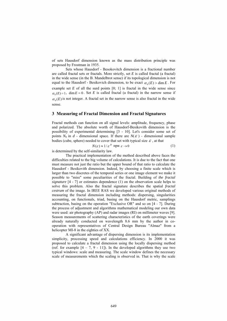
of sets Hausdorf dimension known as the mass distribution principle was proposed by Frostman in 1935.

Sets whose Hausdorf - Besokovitch dimension is a fractional number are called fractal sets or fractals. More strictly, set E is called fractal (a fractal) in the wide sense (in the B. Mandelbrot sense) if its topological dimension is not equal to the Hausdorf - Besikovich dimension, to be exact EE dim)(0 . For

example set E of all the surd points [0; 1] is fractal in the wide sense since 1)(0 E , 0dim E . Set E is called fractal (a fractal) in the narrow sense if

)(0 E is not integer. A fractal set in the narrow sense is also fractal in the wide

sense. 3 Measuring of Fractal Dimension and Fractal Signatures Fractal methods can function on all signal levels: amplitude, frequency, phase and polarized. The absolute worth of Hausdorf-Besikovith dimension is the possibility of experimental determining [3 - 10]. Let's consider some set of points N0 in d - dimensional space. If there are N( ) - dimensional sample bodies (cube, sphere) needed to cover that set with typical size , at that

DN /1)( при 0 (1)

is determined by the self-similarity law. The practical implementation of the method described above faces the

difficulties related to the big volume of calculations. It is due to the fact that one must measure not just the ratio but the upper bound of that ratio to calculate the Hausdorf - Besikovith dimension. Indeed, by choosing a finite scale which is larger than two discretes of the temporal series or one image element we make it possible to "miss" some peculiarities of the fractal. Building of the fractal signature [4 - 7] or estimates dependence (1) on the observation scale helps to solve this problem. Also the fractal signature describes the spatial fractal cestrum of the image. In IREE RAS we developed various original methods of measuring the fractal dimension including methods: dispersing, singularities accounting, on functionals, triad, basing on the Hausdorf metric, samplings subtraction, basing on the operation "Exclusive OR" and so on [4 - 7]. During the process of adjustment and algorithms mathematical modeling our own data were used: air photography (AP) and radar images (RI) on millimeter waves [9]. Season measurements of scattering characteristics of the earth coverings were already naturally conducted on wavelength 8.6 mm by the author in co-operation with representatives of Central Design Bureau "Almaz" from a helicopter MI-8 in the eighties of XX.

A significant advantage of dispersing dimension is its implementation simplicity, processing speed and calculations efficiency. In 2000 it was proposed to calculate a fractal dimension using the locally dispersing method (ref. for example [4 – 7, 9 - 11]). In the developed algorithms they use two typical windows: scale and measuring. The scale window defines the necessary scale of measurements which the scaling is observed in. That is why the scale

649

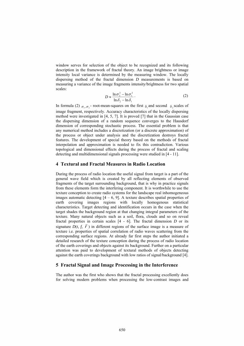
window serves for selection of the object to be recognized and its following description in the framework of fractal theory. An image brightness or image intensity local variance is determined by the measuring window. The locally dispersing method of the fractal dimension D measurements is based on measuring a variance of the image fragments intensity/brightness for two spatial scales:

12

21

22

lnln

lnln

D . (2)

In formula (2) 21, - root-mean-squares on the first

1 and second 2 scales of

image fragment, respectively. Accuracy characteristics of the locally dispersing method were investigated in [4, 5, 7]. It is proved [7] that in the Gaussian case the dispersing dimension of a random sequence converges to the Hausdorf dimension of corresponding stochastic process. The essential problem is that any numerical method includes a discretization (or a discrete approximation) of the process or object under analysis and the discretization destroys fractal features. The development of special theory based on the methods of fractal interpolation and approximation is needed to fix this contradiction. Various topological and dimensional effects during the process of fractal and scaling detecting and multidimensional signals processing were studied in [4 - 11]. 4 Textural and Fractal Measures in Radio Location During the process of radio location the useful signal from target is a part of the general wave field which is created by all reflecting elements of observed fragments of the target surrounding background, that is why in practice signals from these elements form the interfering component. It is worthwhile to use the texture conception to create radio systems for the landscape real inhomogeneous images automatic detecting [4 – 6, 9]. A texture describes spatial properties of earth covering images regions with locally homogenous statistical characteristics. Target detecting and identification occurs in the case when the target shades the background region at that changing integral parameters of the texture. Many natural objects such as a soil, flora, clouds and so on reveal fractal properties in certain scales [4 - 6]. The fractal dimension D or its signature D(t, f, r

) in different regions of the surface image is a measure of

texture i.e. properties of spatial correlation of radio waves scattering from the corresponding surface regions. At already far first steps the author initiated a detailed research of the texture conception during the process of radio location of the earth coverings and objects against its background. Further on a particular attention was paid to development of textural methods of objects detecting against the earth coverings background with low ratios of signal/background [4]. 5 Fractal Signal and Image Processing in the Interference The author was the first who shows that the fractal processing excellently does for solving modern problems when processing the low-contrast images and

650

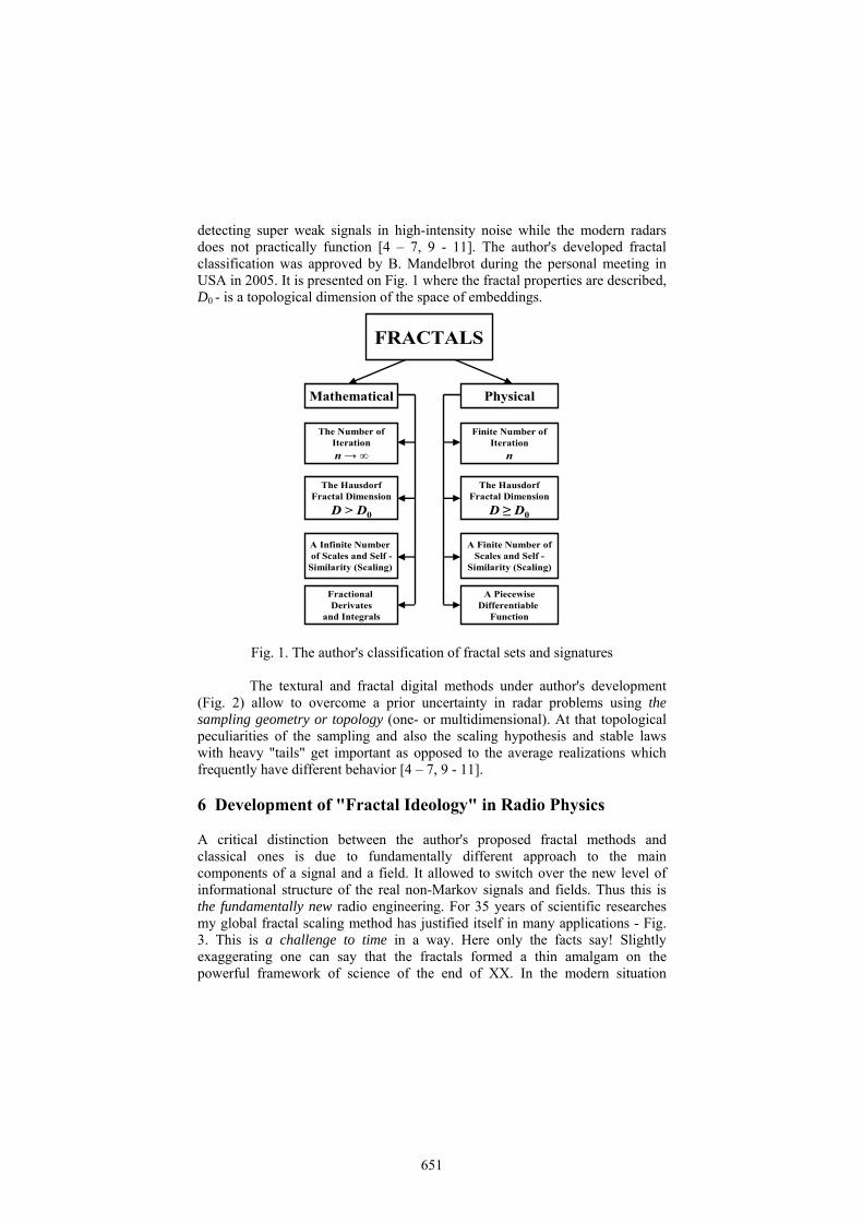
detecting super weak signals in high-intensity noise while the modern radars does not practically function [4 – 7, 9 - 11]. The author's developed fractal classification was approved by B. Mandelbrot during the personal meeting in USA in 2005. It is presented on Fig. 1 where the fractal properties are described, D0 - is a topological dimension of the space of embeddings.

FRACTALS

A Infinite Number оf Scales and Self -

Similarity (Scaling)

The HausdorfFractal Dimension

D > D0

The Number ofIteration

n →∞

Mathematical Physical

The HausdorfFractal Dimension

D ≥ D0

Finite Number ofIteration

n

Fractional Derivates

and Integrals

A Finite Number ofScales and Self -

Similarity (Scaling)

A PiecewiseDifferentiable

Function

Fig. 1. The author's classification of fractal sets and signatures

The textural and fractal digital methods under author's development

(Fig. 2) allow to overcome a prior uncertainty in radar problems using the sampling geometry or topology (one- or multidimensional). At that topological peculiarities of the sampling and also the scaling hypothesis and stable laws with heavy "tails" get important as opposed to the average realizations which frequently have different behavior [4 – 7, 9 - 11]. 6 Development of "Fractal Ideology" in Radio Physics A critical distinction between the author's proposed fractal methods and classical ones is due to fundamentally different approach to the main components of a signal and a field. It allowed to switch over the new level of informational structure of the real non-Markov signals and fields. Thus this is the fundamentally new radio engineering. For 35 years of scientific researches my global fractal scaling method has justified itself in many applications - Fig. 3. This is a challenge to time in a way. Here only the facts say! Slightly exaggerating one can say that the fractals formed a thin amalgam on the powerful framework of science of the end of XX. In the modern situation

651

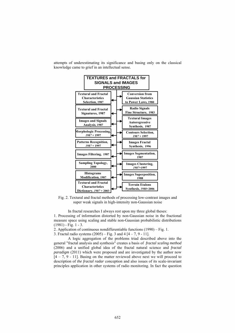
attempts of underestimating its significance and basing only on the classical knowledge came to grief in an intellectual sense.

TEXTURES and FRACTALS for SIGNALS and IMAGES

PROCESSING

Patterns Recognition, 1987 + 1997

Morphologic Processing, 1987 + 1997

Images and Signals Analysis, 1987

Textural and Fractal Signatures, 1987

Textural and Fractal Characteristics Selection, 1987

Conversion from Gaussian Statistics

to Power Laws, 1980

Contours Selection,1987 + 1997

Radio Signals Fine Structure, 1983

Images Filtering, 1987

Images Fractal Synthesis, 1996

Images Segmentation,1987

Textural and Fractal Characteristics

Dictionary, 1987 + 2003

Sampling Topology,2000

Images Superposition,1988

Images Clustering,1987+1997

Textural Images Autoregressive Synthesis, 1987

Terrain Etalons Synthesis, 1988+2006

Histograms Modification, 1987

Fig. 2. Textural and fractal methods of processing low-contrast images and

super weak signals in high-intensity non-Gaussian noise

In fractal researches I always rest upon my three global theses: 1. Processing of information distorted by non-Gaussian noise in the fractional measure space using scaling and stable non-Gaussian probabilistic distributions (1981) - Fig. 1 - 3. 2. Application of continuous nondifferentiable functions (1990) – Fig. 1. 3. Fractal radio systems (2005) – Fig. 3 and 4 [4 – 7, 9 - 11].

A logic aggregation of the problems triad described above into the general "fractal analysis and synthesis" creates a basis of fractal scaling method (2006) and a unified global idea of the fractal natural science and fractal paradigm (2011) which were proposed and are investigated by the author now [4 – 7, 9 - 11]. Basing on the matter reviewed above next we will proceed to description of the fractal radar conception and also issues of its scale-invariant principles application in other systems of radio monitoring. In fact the question

652

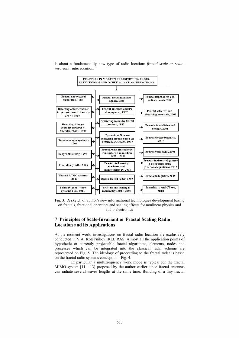
is about a fundamentally new type of radio location: fractal scale or scale-invariant radio location.

Fig. 3. A sketch of author's new informational technologies development basing

on fractals, fractional operators and scaling effects for nonlinear physics and radio electronics

7 Principles of Scale-Invariant or Fractal Scaling Radio Location and its Applications At the moment world investigations on fractal radio location are exclusively conducted in V.A. Kotel’nikov IREE RAS. Almost all the application points of hypothetic or currently projectable fractal algorithms, elements, nodes and processes which can be integrated into the classical radar scheme are represented on Fig. 5. The ideology of proceeding to the fractal radar is based on the fractal radio systems conception - Fig. 4.

In particular a multifrequency work mode is typical for the fractal MIMO-system [11 - 13] proposed by the author earlier since fractal antennas can radiate several waves lengths at the same time. Building of a tiny fractal

653

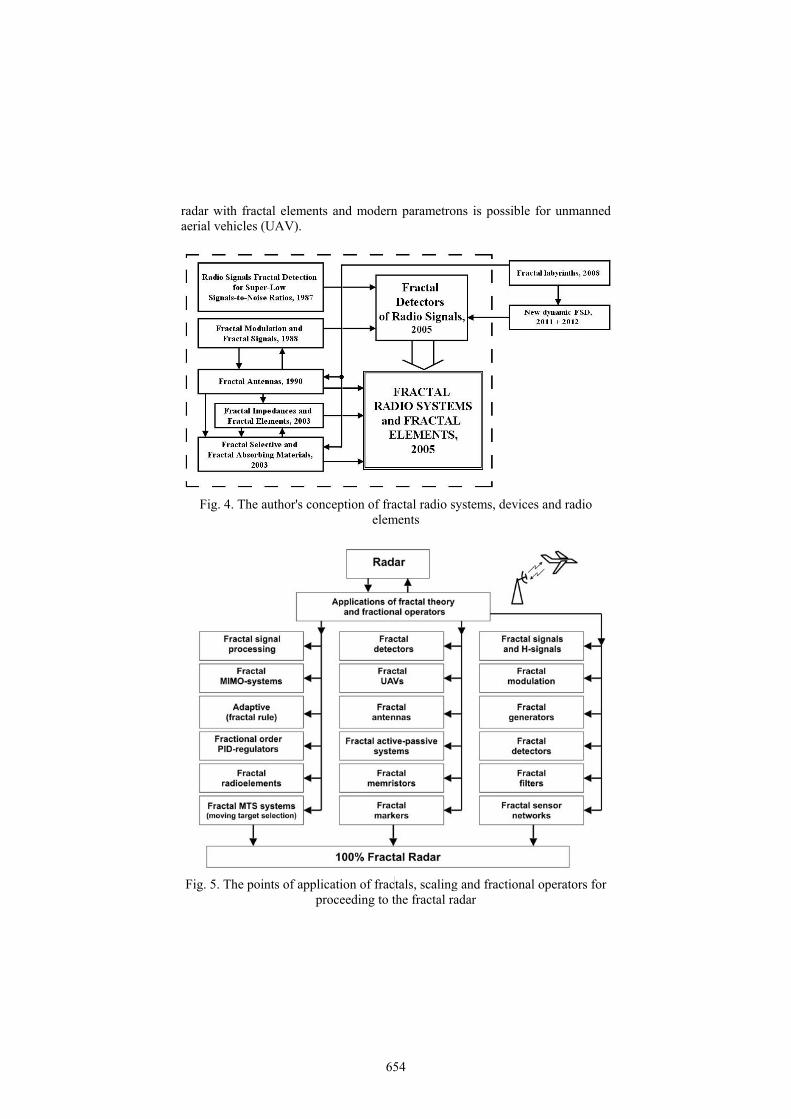
radar with fractal elements and modern parametrons is possible for unmanned aerial vehicles (UAV).

Fig. 4. The author's conception of fractal radio systems, devices and radio

elements

Fig. 5. The points of application of frac tals, scaling and fractional operators for

proceeding to the fractal radar

654

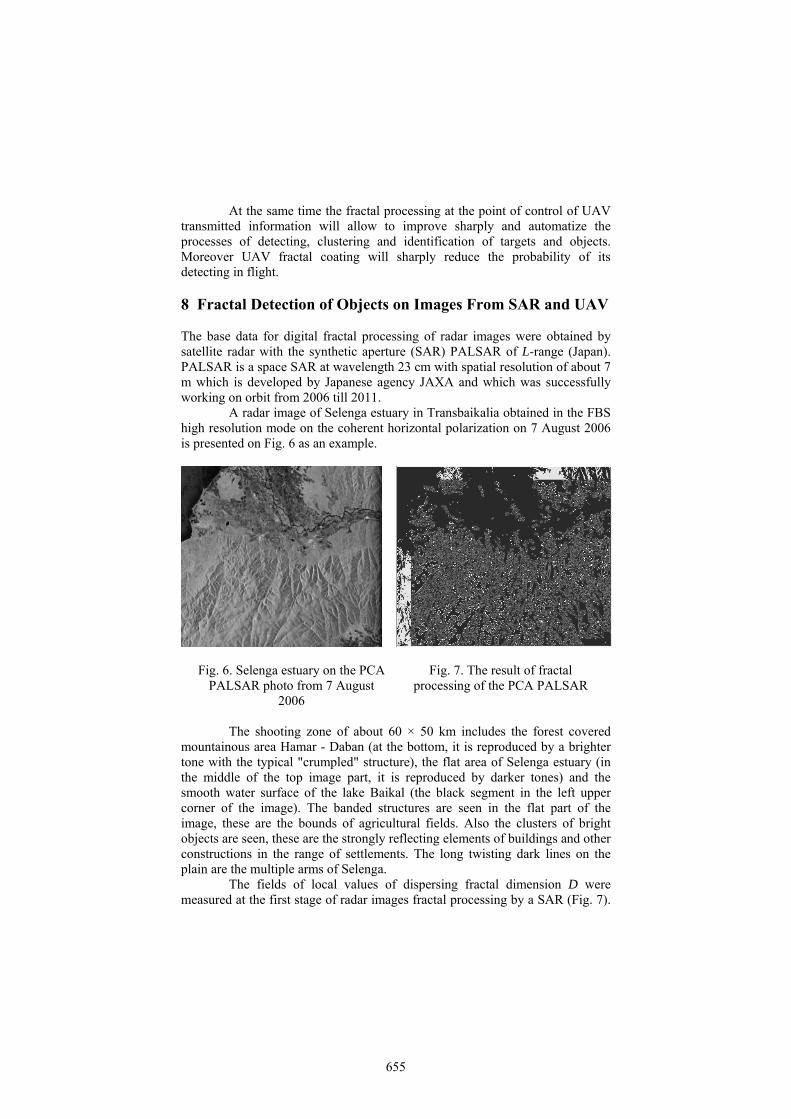
At the same time the fractal processing at the point of control of UAV transmitted information will allow to improve sharply and automatize the processes of detecting, clustering and identification of targets and objects. Moreover UAV fractal coating will sharply reduce the probability of its detecting in flight. 8 Fractal Detection of Objects on Images From SAR and UAV The base data for digital fractal processing of radar images were obtained by satellite radar with the synthetic aperture (SAR) PALSAR of L-range (Japan). PALSAR is a space SAR at wavelength 23 cm with spatial resolution of about 7 m which is developed by Japanese agency JAXA and which was successfully working on orbit from 2006 till 2011.

A radar image of Selenga estuary in Transbaikalia obtained in the FBS high resolution mode on the coherent horizontal polarization on 7 August 2006 is presented on Fig. 6 as an example.

Fig. 6. Selenga estuary on the РСА PALSAR photo from 7 August

2006

Fig. 7. The result of fractal

processing of the РСА PALSAR

The shooting zone of about 60 × 50 km includes the forest covered

mountainous area Hamar - Daban (at the bottom, it is reproduced by a brighter tone with the typical "crumpled" structure), the flat area of Selenga estuary (in the middle of the top image part, it is reproduced by darker tones) and the smooth water surface of the lake Baikal (the black segment in the left upper corner of the image). The banded structures are seen in the flat part of the image, these are the bounds of agricultural fields. Also the clusters of bright objects are seen, these are the strongly reflecting elements of buildings and other constructions in the range of settlements. The long twisting dark lines on the plain are the multiple arms of Selenga.

The fields of local values of dispersing fractal dimension D were measured at the first stage of radar images fractal processing by a SAR (Fig. 7).

655

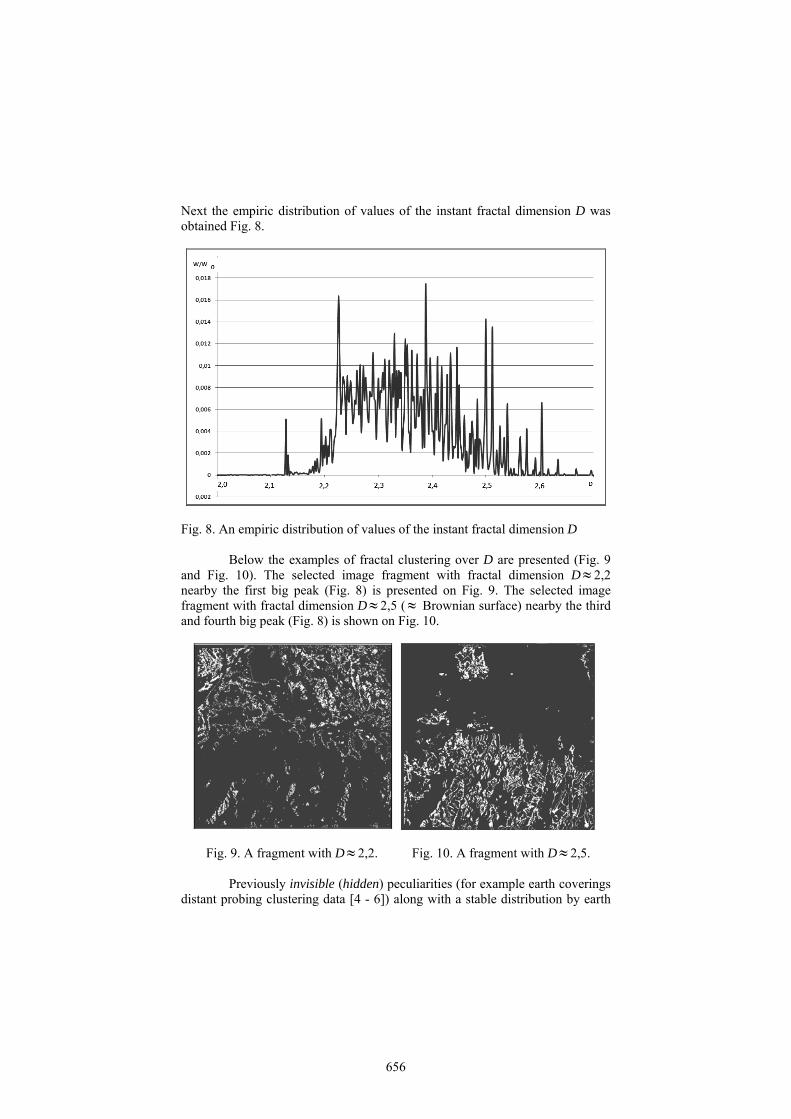
Next the empiric distribution of values of the instant fractal dimension D was obtained Fig. 8.

Fig. 8. An empiric distribution of values of the instant fractal dimension D

Below the examples of fractal clustering over D are presented (Fig. 9

and Fig. 10). The selected image fragment with fractal dimension D 2,2 nearby the first big peak (Fig. 8) is presented on Fig. 9. The selected image fragment with fractal dimension D 2,5 ( Brownian surface) nearby the third and fourth big peak (Fig. 8) is shown on Fig. 10.

Fig. 9. A fragment with D 2,2.

Fig. 10. A fragment with D 2,5.

Previously invisible (hidden) peculiarities (for example earth coverings distant probing clustering data [4 - 6]) along with a stable distribution by earth

656

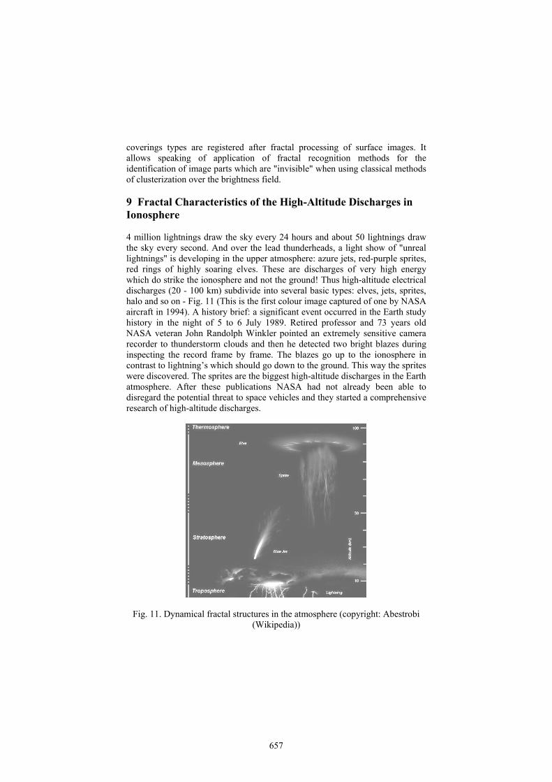
coverings types are registered after fractal processing of surface images. It allows speaking of application of fractal recognition methods for the identification of image parts which are "invisible" when using classical methods of clusterization over the brightness field. 9 Fractal Characteristics of the High-Altitude Discharges in Ionosphere 4 million lightnings draw the sky every 24 hours and about 50 lightnings draw the sky every second. And over the lead thunderheads, a light show of "unreal lightnings" is developing in the upper atmosphere: azure jets, red-purple sprites, red rings of highly soaring elves. These are discharges of very high energy which do strike the ionosphere and not the ground! Thus high-altitude electrical discharges (20 - 100 km) subdivide into several basic types: elves, jets, sprites, halo and so on - Fig. 11 (This is the first colour image captured of one by NASA aircraft in 1994). A history brief: a significant event occurred in the Earth study history in the night of 5 to 6 July 1989. Retired professor and 73 years old NASA veteran John Randolph Winkler pointed an extremely sensitive camera recorder to thunderstorm clouds and then he detected two bright blazes during inspecting the record frame by frame. The blazes go up to the ionosphere in contrast to lightning’s which should go down to the ground. This way the sprites were discovered. The sprites are the biggest high-altitude discharges in the Earth atmosphere. After these publications NASA had not already been able to disregard the potential threat to space vehicles and they started a comprehensive research of high-altitude discharges.

Fig. 11. Dynamical fractal structures in the atmosphere (copyright: Abestrobi (Wikipedia))

657

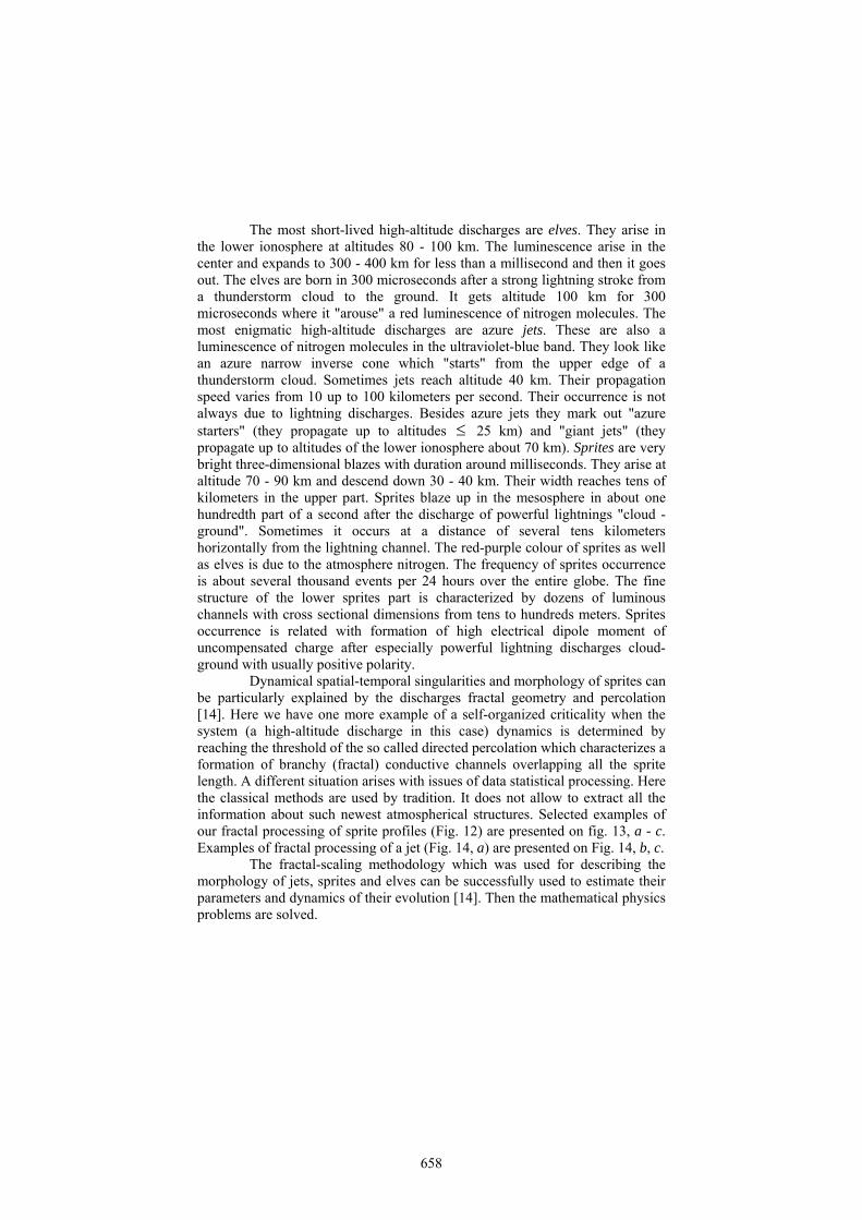
The most short-lived high-altitude discharges are elves. They arise in the lower ionosphere at altitudes 80 - 100 km. The luminescence arise in the center and expands to 300 - 400 km for less than a millisecond and then it goes out. The elves are born in 300 microseconds after a strong lightning stroke from a thunderstorm cloud to the ground. It gets altitude 100 km for 300 microseconds where it "arouse" a red luminescence of nitrogen molecules. The most enigmatic high-altitude discharges are azure jets. These are also a luminescence of nitrogen molecules in the ultraviolet-blue band. They look like an azure narrow inverse cone which "starts" from the upper edge of a thunderstorm cloud. Sometimes jets reach altitude 40 km. Their propagation speed varies from 10 up to 100 kilometers per second. Their occurrence is not always due to lightning discharges. Besides azure jets they mark out "azure starters" (they propagate up to altitudes 25 km) and "giant jets" (they propagate up to altitudes of the lower ionosphere about 70 km). Sprites are very bright three-dimensional blazes with duration around milliseconds. They arise at altitude 70 - 90 km and descend down 30 - 40 km. Their width reaches tens of kilometers in the upper part. Sprites blaze up in the mesosphere in about one hundredth part of a second after the discharge of powerful lightnings "cloud - ground". Sometimes it occurs at a distance of several tens kilometers horizontally from the lightning channel. The red-purple colour of sprites as well as elves is due to the atmosphere nitrogen. The frequency of sprites occurrence is about several thousand events per 24 hours over the entire globe. The fine structure of the lower sprites part is characterized by dozens of luminous channels with cross sectional dimensions from tens to hundreds meters. Sprites occurrence is related with formation of high electrical dipole moment of uncompensated charge after especially powerful lightning discharges cloud-ground with usually positive polarity.

Dynamical spatial-temporal singularities and morphology of sprites can be particularly explained by the discharges fractal geometry and percolation [14]. Here we have one more example of a self-organized criticality when the system (a high-altitude discharge in this case) dynamics is determined by reaching the threshold of the so called directed percolation which characterizes a formation of branchy (fractal) conductive channels overlapping all the sprite length. A different situation arises with issues of data statistical processing. Here the classical methods are used by tradition. It does not allow to extract all the information about such newest atmospherical structures. Selected examples of our fractal processing of sprite profiles (Fig. 12) are presented on fig. 13, a - c. Examples of fractal processing of a jet (Fig. 14, a) are presented on Fig. 14, b, c.

The fractal-scaling methodology which was used for describing the morphology of jets, sprites and elves can be successfully used to estimate their parameters and dynamics of their evolution [14]. Then the mathematical physics problems are solved.

658

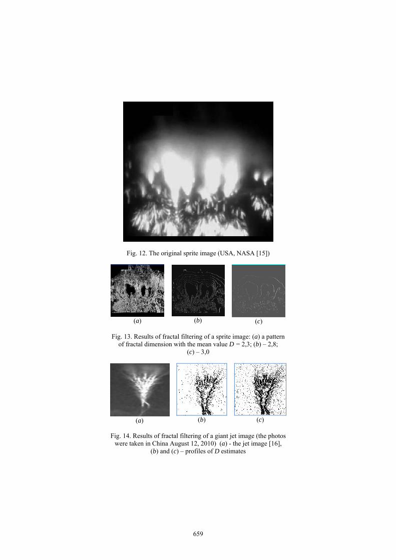
Fig. 12. The original sprite image (USA, NASA [15])

(a)

(b)

(c)

Fig. 13. Results of fractal filtering of a sprite image: (a) a pattern

of fractal dimension with the mean value D = 2,3; (b) – 2,8; (c) – 3,0

(a) (b)

(c)

Fig. 14. Results of fractal filtering of a giant jet image (the photos

were taken in China August 12, 2010) (a) - the jet image [16], (b) and (c) – profiles of D estimates

659

Conclusions The fractal problem in radio location, radio physics and radio engineering is indeed immense. Here I illustrate only fundamental initial issues. It is always hard and even impossible to recede from habitual standards... But the author has good reasons to think that the extensive and valuable material he already obtained and the results of further researches will be used in advanced radio systems. The fractal radio physics, fractal radio engineering and fractal radio location are peculiar radio sciences. They are suffused with a spirit and ideas of the classical radio physics and radio engineering but at the same time they are fundamentally new areas of focus. The results of conducted researches oriented to enhancing the interference immunity of work of radio systems on a radio channel with high-intensity noise and distortion showed opportunities of the approach on the basis of using textural and fractal-scaling methods of detecting and processing random signals and fields.

The author raised these questions back in 1980, and for 35 years has been successfully working on their resolution [4 - 6]. Fractal methods similar to ones presented in this work can be applied when considering wave and oscillatory processes in optics, acoustics and mechanics. Results and conclusions obtained by the author and his pupils have great innovative potential. We think that its realization will resolve a number of current problems of radio physics, radio engineering, radio location, communication and operation and also will allow to provide a new quality for detecting and recognition systems and also development of the new informational technologies.

Many important stages in fractal directions development including the stage of this science field formation have been already passed. However many problems are still to be solved. Results and specific solutions are not of so greatest value like the solution method and its approach are. The method is created by the author [4 - 14]. It is necessary to put it all into practice! References

1. C.A. Rogers. Hausdorff measures, Cambridge University Press, London, 1970, 179

p. 2. K.B. Oldham, J. Spanier. The fractional calculus, Academic Press, New York, 1974,

234 p. 3. B. Mandelbrot. The fractal geometry of nature, W.H. Freeman and co., San

Francisco, 1983, 460 p. 4. A. A. Potapov. Fractals in radiophysics and radar, Logos, Moscow, 2002, 664 p. 5. A. A. Potapov. Fractals in radiophysics and radar: Topology of a sample,

Universitetskaya Kniga, Moscow, 2005, 848 p. 6. A. A. Potapov, in: R. M. Crownover. Introduction to Fractals and Chaos, Moscow:

Tekhnosfera, 2006, p. 374 - 479.

660

7. A. A. Potapov, Yu. V. Gulyaev, S. A. Nikitov, A. A. Pakhomov, and V. A. German, Newest Images Processing Methods, Edited by A.A. Potapov, Moscow, FIZMATLIT, 2008, 496 p.

8. A. A. Potapov, V. A. Chernykh, A. Letnikov Fractional Calculus in the physics of fractals, LAMBERT Academic Publ., Saarbrücken, 2012, 688 p.

9. A.A. Potapov. The textures, fractal, scaling effects and fractional operators as a basis of new methods of information processing and fractal radio systems designing. Proc. SPIE, 7374, p. 73740E-1 - 73740E-14, 2009.

10. A. A. Potapov. Fractal method and fractal paradigm in modern natural science, Nauchnaya Kniga, Voronezh, 2012, 108 p.

11. S.A. Podosenov, A.A. Potapov, J. Foukzon, E.R. Menkova. Nonholonomic, fractal and linked structures in relativistic continuous medium, electrodynamics, quantum mechanics and cosmology: In three volumes, Edited by A.A. Potapov, LENAND, Moscow, 2015, 1128 p.

12. Alexander A. Potapov. Fractals and Scaling in the Radar: A Look from 2015, Book of Abstracts 8nd Int. Conf. (CHAOS’ 2015) on Chaotic Modeling, Simulation and Applications (26 - 29 May 2015, Paris, France), Henri Poincaré Institute, Paris, 2015, p. 102.

13. A.А. Potapov. New Conception of Fractal Radio Device with Fractal Antennas and Fractal Detectors in the MIMO – Systems. Book of Abstracts Third Int. Scientific Symp. “The Modeling of Nonlinear Processes and Systems (MNPS-2015)” (22 – 26 June, 2015, Russia, Moscow, 2015, p. 33.

14. Alexander A. Potapov. Features of Multi-Fractal Structure of the High-Attitude Lightning Discharges in the Ionosphere: Elves, Jets, Sprites, Book of Abstracts 8nd Int. Conf. (CHAOS’ 2015) on Chaotic Modeling, Simulation and Applications (26 - 29 May 2015, Paris, France), Henri Poincaré Institute, Paris, 2015, p. 101 - 102.

15. HTTP://SCIENCE.COMPULENTA.RU/701264/ 16. Yang Jing, Feng GuiLi. A gigantic jet event observed over a thunderstorm in

mainland China. Chinese Science Bulletin, 57, 36, p. 4791 – 4800, 2012.

661

662