A model to estimate economic values of traits in pig breeding

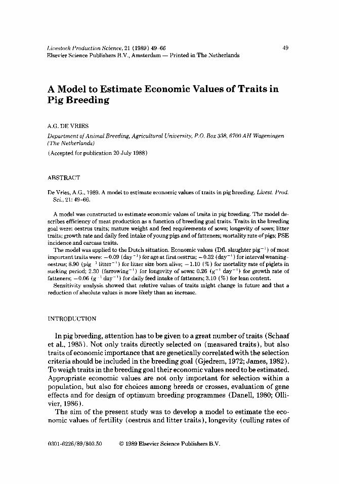
Livestock Production Science, 21 (1989) 49-66 49 Elsevier Science Publishers B.V., Amsterdam - - Printed in The Netherlands

A Model to Est imate Economic Values of Traits in P ig Breed ing

A.G. DE VRIES

Department of Animal Breeding, Agricultural University, P.O. Box 338, 6700 AH Wageningen (The Netherlands)

(Accepted for publication 20 July 1988)

ABSTRACT

De Vries, A.G., 1989. A model to estimate economic values of traits in pig breeding. Livest. Prod. Sci., 21: 49-66.

A model was constructed to estimate economic values of traits in pig breeding. The model de- scribes efficiency of meat production as a function of breeding goal traits. Traits in the breeding goal were: oestrus traits; mature weight and feed requirements of sows; longevity of sows; litter traits; growth rate and daily feed intake of young pigs and of fatteners; mortality rate of pigs; PSE incidence and carcass traits.

The model was applied to the Dutch situation. Economic values (Dfl. slaughter pig- 1 ) of most important traits were: - 0.09 (day- 1 ) for age at first oestrus; - 0.32 (day- 1 ) for interval weaning- oestrus; 8.90 (pig- ~ litter- ~ ) for litter size born alive; - 1.10 (%) for mortality rate of piglets in sucking period; 2.30 (farrowing -~) for longevity of sows; 0.26 (g-~ day -1) for growth rate of fatteners; -0.06 (g-1 day -~ ) for daily feed intake of fatteners; 3.10 (%) for lean content.

Sensitivity analysis showed that relative values of traits might change in future and that a reduction of absolute values is more likely than an increase.

INTRODUCTION

In pig breeding , a t t e n t i o n has to be g iven to a grea t n u m b e r of t r a i t s ( S c h a a f et al., 1985). N o t on ly t r a i t s d i rec t ly se lec ted on ( m e a s u r e d t r a i t s ) , bu t also t r a i t s o f economic i m p o r t a n c e t h a t are gene t ica l ly co r re l a t ed wi th t he se lect ion cr i te r ia should be inc luded in the b reed ing goal (Gjedrem, 1972; J a m e s , 1982 ). To weigh t r a i t s in t he b reed ing goal t he i r economic va lues need to be e s t ima ted . A p p r o p r i a t e economic va lues are no t on ly i m p o r t a n t for se lec t ion wi th in a popu la t ion , bu t also for choices a m o n g b reeds or crosses, eva lua t ion of gene effects a n d for design of o p t i m u m b reed ing p r o g r a m m e s (Danel l , 1980; Olli- vier, 1986 ).

T h e a im of the p r e s e n t s t udy was to develop a mode l to e s t i m a t e the economic va lues of fer t i l i ty (oes t rus a n d l i t te r t r a i t s ) , longevi ty (cul l ing ra tes of

0301-6226/89/$03.50 © 1989 Elsevier Science Publishers B.V.

50

sows) and production traits (growth performance and carcass quality). The values are used to define a breeding goal for within-population selection that is optimal for the pig industry. The model can be used in many situations. In this paper an application is given for the situation in The Netherlands. The relative figures of the results of this application are probably not much different from the values of traits in other European countries. A study of effects of changes in economic parameters and in technical results on economic values is included.

METHOD

Conditions and strategy

Smith et al. (1986) imposed two conditions for derivation of economic values. The first is that extra profit resulting from extra output should be excluded. The second is that changes that correct previous inefficiency in the production enterprise should not be counted. A third condition for development of the present model has been that limitations of individual farms are not considered. If, for example, piglets reach their optimal weaning weight as a result of selection one day earlier, most farmers would not shorten the length of the suckling period, because they wean on a fixed day of the week. However, when a group of farms is considered, this limitation is not relevant, because there would also be some farmers who could now wean a week earlier. There- fore, average weaning age of the group of farms would be reduced.

For some traits (e.g. lean meat percentage), the economic value is not only influenced by the mean level but also by the variation between animals. This was taken into account in the model.

One of the methods of deriving economic values is to use profit or efficiency equations (Danell, 1980; Brascamp, 1983). The economic value of a trait is calculated as the ratio of the change in profit (or efficiency) to a small change in genetic level of the trait. The equations can be based on individual efficiency, on dam-progeny efficiency or on herd efficiency (Elsen et al., 1986).

Danell (1980) gives a lot of examples of studies where economic values were calculated based on effects of traits on producer's profit. However, such a basis would give a violation of the first condition of Smith et al. (1986). An appropriate way to cope with the conditions of Smith et al. (1986) is to derive economic values based on efficiency of production (cost per unit of product), and to regard all costs as variable with the level of output. This strategy was followed in the present study.

Model description

The model simulated the performance of a group of sows and their offspring. Efficiency of production was calculated as total net costs kg- 1 offspring output

51

(kg carcass weight) minus adjustment of price for carcass quality. Total net costs was defined as sow costs minus returns for culled sows plus costs for offspring

efficiency = (total net costs/offspring output) - adjustment of price total net costs = sow c o s t s - sow returns + offspring costs

The traits studied with the model can be seen in Table 6. For each trait, the effect of a small change in level of performance on efficiency of production (kg-~ carcass weight) was calculated. Change in efficiency was expressed on a slaughter pig -1 basis (change in efficiency slaughter pig -1 produced), to assist in a bet ter interpretation of results. These values were derived by mul- tiplication of change in efficiency with initial offspring output slaughter p ig- 1. The economic value of a trait was calculated as

( change in efficiency slaughter p ig- 1 ) / (change of trait )

The computer model is writ ten in Fortran-77. Equations for calculation of sow costs and returns, offspring costs and output and adjustment of price are given in Appendix A.

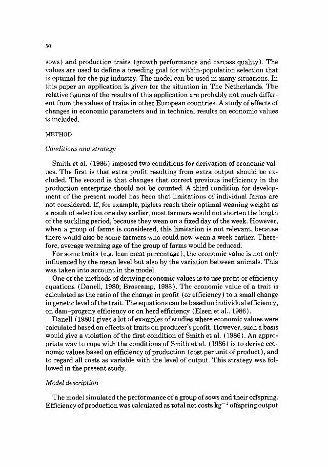
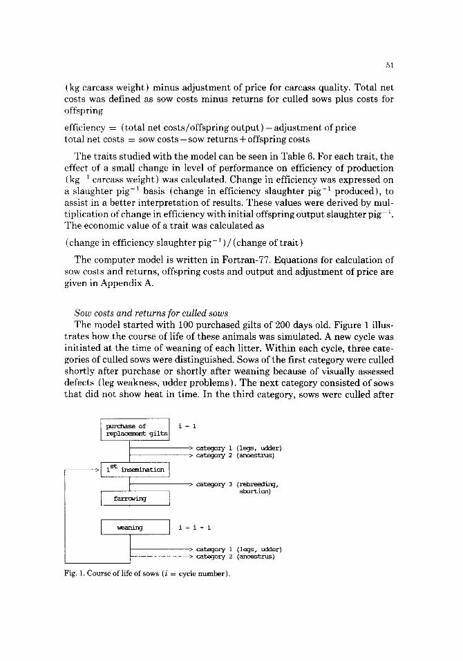
Sow costs and returns for culled sows The model started with 100 purchased gilts of 200 days old. Figure 1 illus-

trates how the course of life of these animals was simulated. A new cycle was initiated at the time of weaning of each litter. Within each cycle, three categories of culled sows were distinguished. Sows of the first category were culled shortly after purchase or shortly after weaning because of visually assessed defects (leg weakness, udder problems). The next category consisted of sows that did not show heat in time. In the third category, sows were culled after

purchase of gilts replacement

- - > I ist insemination I

I i l

I I l

i=i

• > category i (legs, udder) -> category 2 (anoestrus)

-> category 3 (rebreeding, abortion)

i=i+l

-> category 1 (legs, udder) -> category 2 (anoestrus)

Fig. 1. Course of life of sows (i = cycle number).

52

one or more unsuccessful inseminations. After cycle Number 10, all remaining sows were sold shortly after weaning (Category 1 ).

Sow costs were calculated from the following components: (a) purchase costs replacement gilt-1 (representing all costs gilt-1 made by

the breeder); (b) basic non-feed costs day -1 (labour, management, housing, interest on

livestock investment, water, electricity and miscellaneous); (c) basic feed costs day- 1 (requirements for growth and maintenance ); (d) extra non-feed costs farrowing-1 (labour, management, veterinary and

heating costs; extra costs for housing before and after lactation ); (e) extra non-feed costs lactation day-1 (extra costs for housing); (f) breeding costs first insemination-1; (g) feed costs for development of gestation products pig-1 born; (h) feed costs for milk production per lactation day pig-1 weaned; (i) costs associated with selling of sows.

Basic costs day- 1 (Components (b) and (c) ) were specified for 3 age categories: - - replacement gilts, from time of purchase to first insemination; - - gilts, from time of first insemination to first farrowing; - - sows, after first farrowing. Extra costs for housing (Components (d) and (e)) reflected the difference between costs place-1 in the farrowing house and costs place-1 in the breeding/gestation house.

Weight differences between culling categories were assumed to be due only to differences in maturity. (The effect of recovering from weight losses during lactation on liveweight gain was excluded. ) Carcass price kg- 1 for culled sows was dependent on cycle number.

When age at first oestrus or interval weaning-oestrus changes, state of maturity of culled sows also changes. This needs to be included when economic values of these traits are calculated. Therefore, liveweight of sows in each cycle was adjusted by the value for growth rate in that cycle multiplied by the change in age

Awsi = ~afoe*grsi + ( i-- 1 ) ,A iwoe ,grs i

where: Awsi = change in weight of sows; Aafoe = change in age at first oestrus; Aiwoe = change in interval weaning-oestrus (all cycles); grsi = growth rate of sows in Cycle No. i; i = cycle number.

Offspring costs and output Three growing stages were distinguished for the offspring of the sows:

- - from birth to weaning (Stage 1 ); - - from weaning to feeder pig weight (Stage 2 ); - - from feeder pig weight to slaughter weight (Stage 3 ).

53

Birth weight, weaning weight, feeder pig weight and slaughter weight were fixed.

Offspring costs were calculated from: (a) feed costs day-1 in each of these stages; (b) non-feed costs day-1 in Stages 2 and 3 (labour, management, housing,

interest on livestock investment, water, heating, electricity and miscellaneous ); (c) extra costs pig -1 weaned in Stage 1 (iron injection, castration, tail

cutting); (d) extra costs in Stage 3 feeder pig -1 (transportation of feeder pigs, vet-

erinary costs, labour, management and housing costs during empty days between batches);

(e) costs associated with selling of slaughter pigs. For animals that died during Stages 2 or 3 half of the feed and the time-

dependent non-feed costs in that particular stage were counted. Total number of piglets weaned was reduced by mortality in Stages 2 and 3

to give total number of slaughter pigs. Output (kg carcass weight) per PSE- free pig was fixed, but output per pig with PSE-syndrome indications was reduced by a specified percentage (transport death, weight loss).

Adjustment of price for carcass quality The Dutch classification system for carcass quality is a dual grading system

according to estimated lean meat percentage (ELMP) and according to type classes: C (negligible numbers ), B, A and AA. Basic prices refer to 52 % ELMP and Type A, with reductions for lower and premiums for higher classes.

Average adjustment of price for ELMP is a function of the fraction of carcasses in Group 1 (ELMP < 52%) and Group 2 (ELMP 1> 52% ) and the average ELMP of each group.

The approach for calculation of change in price owing to shifts in type classes was based on the strategy for derivation of economic ~¢alues for categorical traits (Danell, 1980; Danell and RSnningen, 1981). The distribution for the underlying scale was defined with the truncation points that correspond with the frequencies of Type B and AA in the basic situation. The change in frequency of Type B was calculated as - Atype • zB/(zB + zAA ), while change in frequency of Type AA was calculated as +Atype . zAA/(zB + zAA ), where A type is shift in type class and zB and zAA are the heights of the distribution ordinate for Type B and Type AA, respectively.

Levels of genetic traits and parameters (basic situation)

The model was applied to the situation in The Netherlands. Parameters originate from different Dutch sources and are close to the real situation in 1987.

Culling percentages of purchased gilts for Categories 1, 2 and 3 were 1, 3 and

54

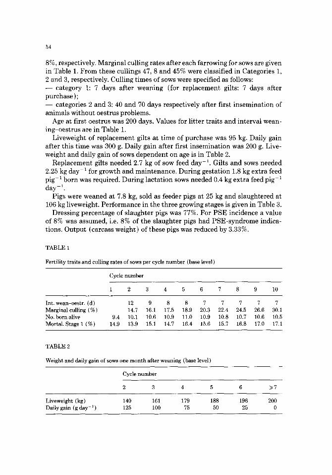
8%, respectively. Marginal culling rates after each farrowing for sows are given in Table 1. From these cullings 47, 8 and 45% were classified in Categories 1, 2 and 3, respectively. Culling times of sows were specified as follows: - - category 1 : 7 days after weaning (for replacement gilts: 7 days after purchase ); - - categories 2 and 3:40 and 70 days respectively after first insemination of animals without oestrus problems.

Age at first oestrus was 200 days. Values for litter traits and interval weaning-oestrus are in Table 1.

Liveweight of replacement gilts at time of purchase was 95 kg. Daily gain after this time was 300 g. Daily gain after first insemination was 200 g. Live- weight and daily gain of sows dependent on age is in Table 2.

Replacement gilts needed 2.7 kg of sow feed day -1. Gilts and sows needed 2.25 kg day- 1 for growth and maintenance. During gestation 1.8 kg extra feed pig- 1 born was required. During lactation sows needed 0.4 kg extra feed pig- 1 day- 1.

Pigs were weaned at 7.8 kg, sold as feeder pigs at 25 kg and slaughtered at 106 kg liveweight. Performance in the three growing stages is given in Table 3.

Dressing percentage of slaughter pigs was 77%. For PSE incidence a value of 8% was assumed, i.e. 8% of the slaughter pigs had PSE-syndrome indications. Output (carcass weight) of these pigs was reduced by 3.33%.

TABLE1

Fertility traits and culling rates of sows per cycle number (base level)

Cycle number

1 2 3 4 5 6 7 8 9 10

Int. wean-oestr. (d) 12 9 8 8 7 7 7 7 7 Marginal culling (%) 14.7 16.1 17.5 18.9 20.3 22.4 24.5 26.6 30.1 No. born alive 9.4 10.1 10.6 10.9 11.0 10.9 10.8 10.7 10.6 10.5 Mortal. Stage 1 (%) 14.9 13.9 15.1 14.7 16.4 15.6 15.7 16.8 17.0 17.1

TABLE 2

Weight and daily gain of sows one month after weaning (base level)

Cycle number

2 3 4 5 6 >/7

Liveweight (kg) 140 161 179 188 196 200 Daily gain (g day- 1 ) 125 100 75 50 25 0

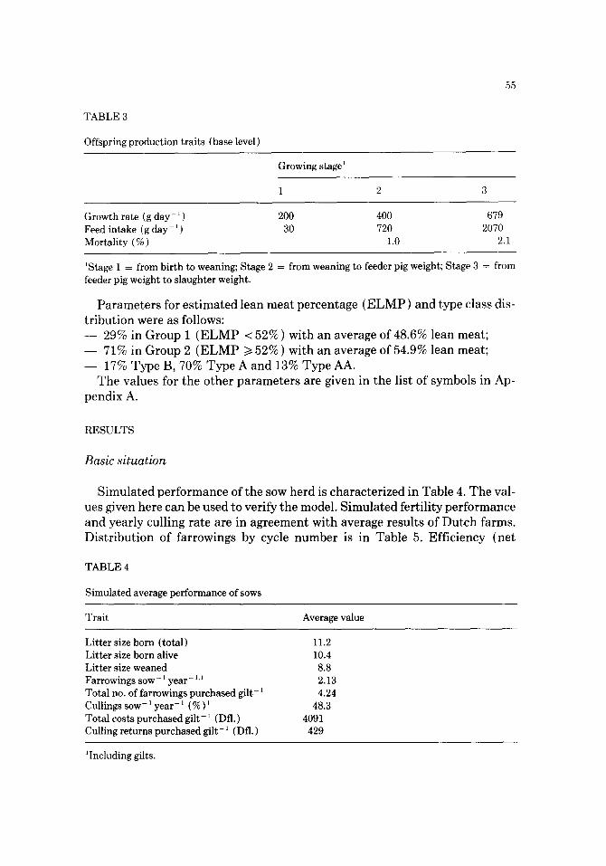
TABLE 3

Offspring production traits {base level)

55

Growing stage'

1 2 3

Growth rate (g day- ~ ) 200 400 679 Feed intake (g day- 1 ) 30 720 2070 Mortality (%) 1.0 2.1

~Stage 1 = from birth to weaning; Stage 2 = from weaning to feeder pig weight; Stage 3 -- from feeder pig weight to slaughter weight.

P a r a m e t e r s for e s t i m a t e d lean m e a t p e r c e n t a g e ( E L M P ) and type class dis- t r i bu t ion were as follows: - - 29% in G r o u p 1 ( E L M P < 52% ) wi th an average of 48.6% lean mea t ; - - 71% in G r o u p 2 ( E L M P >~ 52% ) wi th an average of 54.9% lean mea t ; - - 17% T y p e B, 70% T y p e A a n d 13% T y p e AA.

T h e va lues for the o the r p a r a m e t e r s are given in the list of symbols in Ap- pend ix A.

RESULTS

Basic situation

S i m u l a t e d p e r f o r m a n c e of the sow he rd is cha rac t e r i zed in Tab l e 4. T h e values given here can be used to ver i fy the model . S i m u l a t e d fer t i l i ty p e r f o r m a n c e and yea r ly cul l ing ra te are in a g r e e m e n t wi th ave rage resu l t s of D u t c h fa rms . D i s t r i bu t ion of fa r rowings by cycle n u m b e r is in Tab le 5. Ef f ic iency (ne t

TABLE4

Simulated average performance of sows

Trait Average value

Litter size born {total) 11.2 Litter size born alive 10.4 Litter size weaned 8.8 Farrowings sow- ' year- ~'~ 2.13 Total no. of farrowings purchased gilt- ' 4.24 Cullings sow- ' year- 1 ( % ) 1 48.3 Total costs purchased gilt- ' (Dfl.) 4091 Culling returns purchased gilt- ' (Dfl.) 429

Including gilts.

56

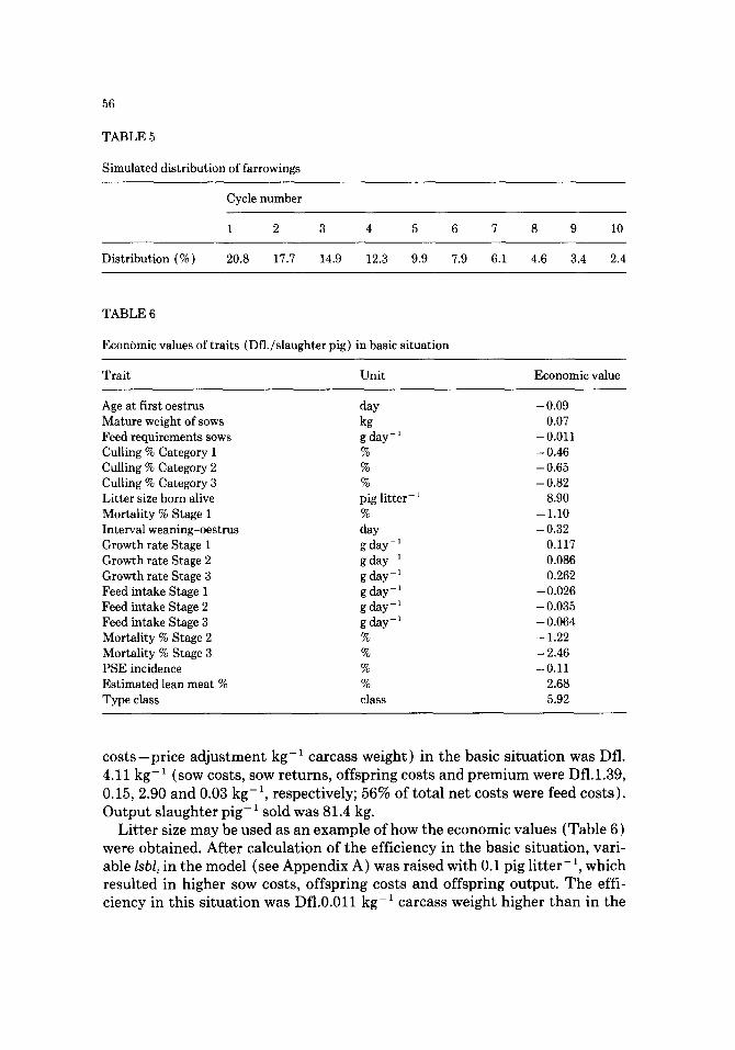
TABLE 5

Simulated distribution of farrowings

Cycle number

1 2 3 4 5 6 7 8 9 10

Distribution (9 ) 20.8 17.7 14.9 12.3 9.9 7.9 6.1 4.6 3.4 2.4

TABLE 6

EconOmic values of traits {Dfl./slaughter pig) in basic situation

Trait Unit Economic value

Age at first oestrus day -0.09 Mature weight of sows kg 0.07 Feed requirements sows g day- 1 - 0.011 Culling % Category 1 % -0.46 Culling % Category 2 % - 0.65 Culling % Category 3 % - 0.82 Litter size born alive pig litter- 1 8.90 Mortality % Stage 1 % - 1.10 Interval weaning-oestrus day - 0.32 Growth rate Stage 1 g day-1 0.117 Growth rate Stage 2 g day- 1 0.086 Growth rate Stage 3 g day- 1 0.262 Feed intake Stage 1 g day- ~ - 0.026 Feed intake Stage 2 g day- 1 - 0.035 Feed intake Stage 3 g day- 1 - 0.064 Mortality % Stage 2 % - 1.22 Mortality % Stage 3 % - 2.46 PSE incidence % - 0.11 Estimated lean meat % % 2.68 Type class class 5.92

c o s t s - p r i c e a d j u s t m e n t k g - 1 ca rcas s we igh t ) in t he bas ic s i t u a t i o n was Dfl.

4.11 kg -1 (sow costs , sow r e t u r n s , o f f sp r ing cos ts a n d p r e m i u m were Df l . l .39 ,

0.15, 2.90 a n d 0.03 k g - 1 , r e spec t ive ly ; 56% of t o t a l ne t cos ts were feed cos t s ) .

O u t p u t s l a u g h t e r p i g - 1 so ld was 81.4 kg. L i t t e r size m a y be u sed as an e x a m p l e of how t h e economic va lues (Tab l e 6)

were ob ta ined . Af t e r c a l c u l a t i o n of t he e f f ic iency in t he bas ic s i t ua t i on , var i -

ab le Isbli in t he mode l (see A p p e n d i x A ) was r a i sed wi th 0.1 p ig l i t t e r - 1 , wh ich

r e s u l t e d in h ighe r sow costs , o f f sp r ing cos ts a n d o f f sp r ing ou tpu t . T h e effi- c i ency in th i s s i t u a t i o n was Dfl.0.011 k g - 1 ca rcass we igh t h ighe r t h a n in t he

57

basic situation. Multiplied with output slaughter pig-1 and divided by 0.1 pig l i t ter- 1, this gave an economic value of Dfl.8.90 for litter size born alive.

The economic value for each trait in Table 6 was calculated under the condition that performance levels of all other traits in the table remained constant.

When gilts showed first oestrus 1 day earlier, sow costs were reduced and returns for culled gilts and sows were somewhat lower, because animals were a day younger when culled.

An increase of 1 kg in mature weight (base level = 200 kg) meant 0.5% more returns for culled sows, because weight and daily gain in each reproduction cycle were increased by 0.5%.

When marginal culling rate in each reproduction cycle was lowered by 1%, there were 4 effects. The first one was a small change in average litter size weaned ( + 0.008 pigs l i t ter- 1) owing to an increase in average cycle number. Secondly, the difference between costs for ready-to-mate gilts and returns for cullings was spread over more litters (+0.20 litters gilt-~). The other two effects were a higher farrowing index (farrowings sow -1 year -1) and an increase of returns for cullings. These effects were different for each of the 3 culling categories due to the differences in culling time (see section 2.3).

With higher litter size or lower mortali ty rate in the suckling period, sow costs (excluding feed costs for development of gestation products and milk production) and returns for cullings were spread over more offspring. Average litter size weaned was raised by 0.085 pig per 0.1 pig extra born alive, while 1% lower mortali ty rate raised litter size weaned by 0.104 pig.

For 47% of the sows (culling Category 1 ) interval weaning-oestrus was not important in their last reproduction cycle. As a result, 0.9 sow days per reproduction cycle were saved for each day shorter interval, which reduced basic sows costs. Because of a lower age of culled sows, returns for cullings were slightly reduced.

A higher growth rate of piglets during suckling (Stage 1 ) reduced the length of this period. Basic sow costs, extra costs during lactation, sow feed costs for milk production and pig feed costs were reduced.

A higher growth rate in Stage 2 (weaners) or Stage 3 (fatteners) reduced t ime-dependent feed and non-feed costs.

Economic value of a 1% lower mortali ty rate for Stage 2 and for Stage 3 corresponded with 1% of the cumulated costs of the animals at death. The economic value of a 1% lower PSE incidence corresponded with 0.0333% (3.33 X 1% ) of total costs slaughter pig- 1.

When average estimated lean meat percentage was improved by 1%, price adjustment kg- 1 carcass weight was increased by 29% • (price reduction below 52% ) + 71% • (price increase above 52% ). An average shift of 0.01 type classes resulted in 0.54% decrease of frequency of Type B and 0.46% increase of frequency of Type AA.

58

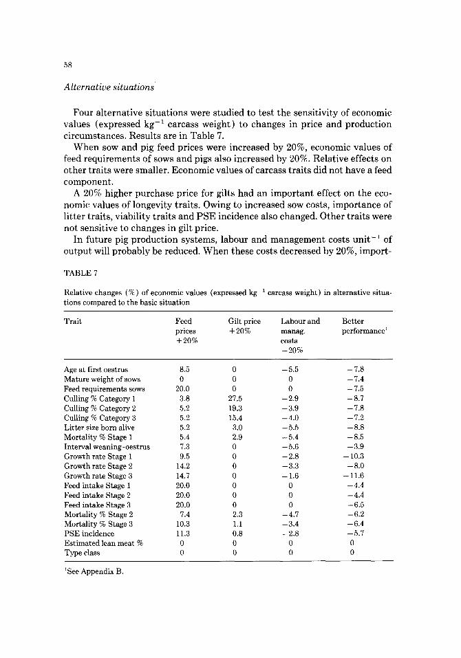
Alternative situations

Four alternative situations were studied to test the sensitivity of economic values (expressed kg-1 carcass weight) to changes in price and production circumstances. Results are in Table 7.

When sow and pig feed prices were increased by 20%, economic values of feed requirements of sows and pigs also increased by 20%. Relative effects on other traits were smaller. Economic values of carcass traits did not have a feed component.

A 20% higher purchase price for gilts had an important effect on the economic values of longevity traits. Owing to increased sow costs, importance of litter traits, viability traits and PSE incidence also changed. Other traits were not sensitive to changes in gilt price.

In future pig production systems, labour and management costs unit-1 of output will probably be reduced. When these costs decreased by 20%, import-

T A B L E 7

Relative changes (%) of economic values (expressed kg-~ carcass weight) in alternative situa- t ions compared to the basic s i tuat ion

Tra i t Feed Gilt price Labour and Bet ter prices + 20% manag, performance ~

+ 20% costs - 2 0 %

Age at first oestrus 8.5 0 - 5.5 - 7.8 Mature weight of sows 0 0 0 - 7.4 Feed requirements sows 20.0 0 0 - 7.5

Culling % Category 1 3.8 27.5 - 2 . 9 - 8 . 7 Culling % Category 2 5.2 19.3 - 3.9 - 7.8 Culling % Category 3 5.2 15.4 - 4.0 - 7.2 Lit ter size born alive 5.2 3.0 - 5.5 - 8.8 Mortal i ty % Stage 1 5.4 2.9 - 5.4 - 8.5 Interval weaning-oes t rus 7.3 0 - 5.6 - 3.9 Growth rate Stage 1 9.5 0 - 2 . 8 - 10.3 Growth rate Stage 2 14.2 0 - 3 . 3 - 8 . 0 Growth rate Stage 3 14.7 0 - 1.6 - 11.6

Feed intake Stage 1 20.0 0 0 - 4.4 Feed intake Stage 2 20.0 0 0 - 4.4 Feed intake Stage 3 20.0 0 0 - 6 . 5 Mortal i ty % Stage 2 7.4 2.3 - 4 . 7 - 6 . 2 Mortal i ty % Stage 3 10.3 1.1 - 3 . 4 - 6 . 4 PSE incidence 11.3 0.8 - 2.8 - 5.7 Es t imated lean meat % 0 0 0 0 Type class 0 0 0 0

'See Appendix B.

59

ance of fertility and longevity traits decreased. Effects on the economic values for growth rate were relatively small, especially for growth rate in the fattening period.

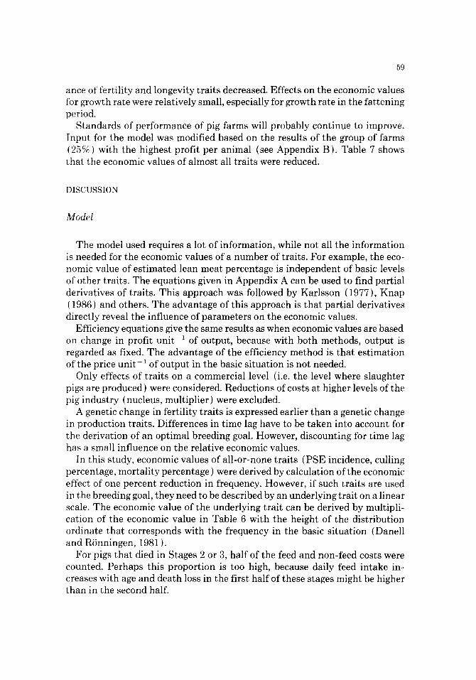
Standards of performance of pig farms will probably continue to improve. Input for the model was modified based on the results of the group of farms (25%) with the highest profit per animal (see Appendix B). Table 7 shows that the economic values of almost all traits were reduced.

DISCUSSION

Model

The model used requires a lot of information, while not all the information is needed for the economic values of a number of traits. For example, the economic value of estimated lean meat percentage is independent of basic levels of other traits. The equations given in Appendix A can be used to find partial derivatives of traits. This approach was followed by Karlsson (1977), Knap (1986) and others. The advantage of this approach is that partial derivatives directly reveal the influence of parameters on the economic values.

Efficiency equations give the same results as when economic values are based on change in profit unit-1 of output, because with both methods, output is regarded as fixed. The advantage of the efficiency method is that estimation of the price uni t - 1 of output in the basic situation is not needed.

Only effects of traits on a commercial level (i.e. the level where slaughter pigs are produced) were considered. Reductions of costs at higher levels of the pig industry (nucleus, multiplier) were excluded.

A genetic change in fertility traits is expressed earlier than a genetic change in production traits. Differences in time lag have to be taken into account for the derivation of an optimal breeding goal. However, discounting for time lag has a small influence on the relative economic values.

In this study, economic values of all-or-none traits (PSE incidence, culling percentage, mortality percentage ) were derived by calculation of the economic effect of one percent reduction in frequency. However, if such traits are used in the breeding goal, they need to be described by an underlying trait on a linear scale. The economic value of the underlying trait can be derived by multipli- cation of the economic value in Table 6 with the height of the distribution ordinate that corresponds with the frequency in the basic situation (Danell and RSnningen, 1981 ).

For pigs that died in Stages 2 or 3, half of the feed and non-feed costs were counted. Perhaps this proportion is too high, because daily feed intake in- creases with age and death loss in the first half of these stages might be higher than in the second half.

60

Economic values of traits for within population selection

The economic values in Table 6 can be used for evaluation of breeds or gene effects and are important for optimization of selection within a population. Absolute economic values always apply to specific production conditions, in this case in The Netherlands, but the relative figures are also useful for other European countries.

The most relevant traits for within-population selection in Dutch pig breeding programmes are: age at first oestrus, interval weaning-oestrus; litter size born alive; mortality rate during suckling; growth rate and feed intake in the fattening period; lean content and longevity of sows related to leg and udder quality (Kanis, 1985; Knap et al., 1985; Knap, 1986). Other traits in Table 6 are probably correlated with these traits: - - culling percentage due to anoestrus is positively correlated with age at first oestrus and interval weaning-oestrus;

- - growth rate of young piglets is negatively correlated with litter size (owing to a lower milk consumption pig- 1 ) (Ritter et al, 1985; van der Steen, 1986); - - mature weight and feed requirements of sows are positively correlated with growth rate of fatteners, which is unfavourable (assuming that 1 kg heavier sows need 10 g day -1 more feed, see Table 6); - - growth rates in Stages 1 and 2 are positively correlated with growth rate in Stage 3;

- - viability traits and PSE incidence are positively correlated with lean content. For an appropriate weighting of the traits in selection, more information

about these correlations is needed. Based on Averdunk et al. (1983), a 1% increase in lean content will give

0.7% improvement of estimated lean meat percentage. The C.O.V. (1976) re- ported for the regression of type on lean content a value of 0.285 type classes percentage- 1 lean content. In the current situation this regression is probably lower, because of a reduced variation in type. Therefore, a regression of 0.2 type classes percentage -1 lean content is expected (E. Kanis, personal com- munication, 1986). So when lean content is used as a trait in the breeding goal instead of ELMP and type, its economic value (slaughter pig -1) is Dfl.3.10 percentage- 1 (0.7 • 2.68 + 0.2 • 5.92 ).

Usually longevity is expressed as number of farrowings purchased gilt- 1. A reduction of culling rate of 1% in each cycle corresponded with 0.2 extra farrowings purchased gilt -1. This means that the economic value (expressed slaughter pig- 1 ) of longevity for Category 1 is Dfl.2.30 farrowing- 1 (0.46/0.2).

For fertility traits (litter size, mortality percentage in the suckling period and interval weaning-oestrus) Table 5 can be used to calculate the economic effects cycle number-1 separately. This can be useful particularly for the first cycle number, because the genetic correlation between size of the first litter and size of older litters is not equal to 1 (Knap, 1986; Vangen, 1986).

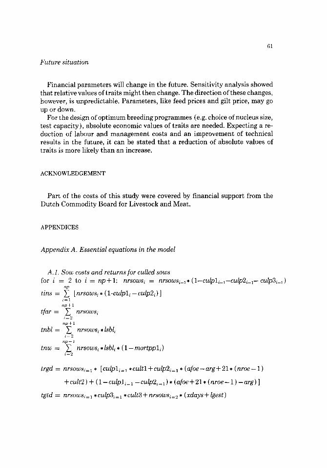
Future s i tuat ion

61

Financial parameters will change in the future. Sensitivity analysis showed that relative values of traits might then change. The direction of these changes, however, is unpredictable. Parameters, like feed prices and gilt price, may go up or down.

For the design of optimum breeding programmes (e.g. choice of nucleus size, test capacity), absolute economic values of traits are needed. Expecting a reduction of labour and management costs and an improvement of technical results in the future, it can be stated that a reduction of absolute values of traits is more likely than an increase.

ACKNOWLEDGEMENT

Part of the costs of this study were covered by financial support from the Dutch Commodity Board for Livestock and Meat.

APPENDICES

Append ix A. Essent ial equations in the model

A. 1. Sow costs and returns for culled sows for i = 2 to i = np+ l : nrsowsi = nrsowsi_~, (1-culpl i_l-CUlp2i_l-CUlp3i_~)

np

t ins = ~ [nrsowsi * ( 1 - c u l p l i - c u l p 2 i ) ] i=1 rip+ 1

tfar = ~, nrsowsi i = 2

rip+ 1

t n b l = ~ nrsowsi , lsbl i i = 2

n p + 1

tnw = ~. nrsowsi , l sb l i* (1-mor tppl l ) i = 2

trgd =

tgtd =

nrsowsi=l * [culpli=l , c u l t l +culp2i=l * ( a f o e - a r g + 2 1 , ( n r o e - 1 )

+cul t2 ) + ( 1 - c u l p l i = l - c u l p 2 i = l ) * ( a l o e + 2 1 , ( n r o e - 1 ) - a r g ) ]

nrsowsi = ~ * culp3i = 1 * cult3 + nrsowsi = 2 * ( xdays + Igest )

62

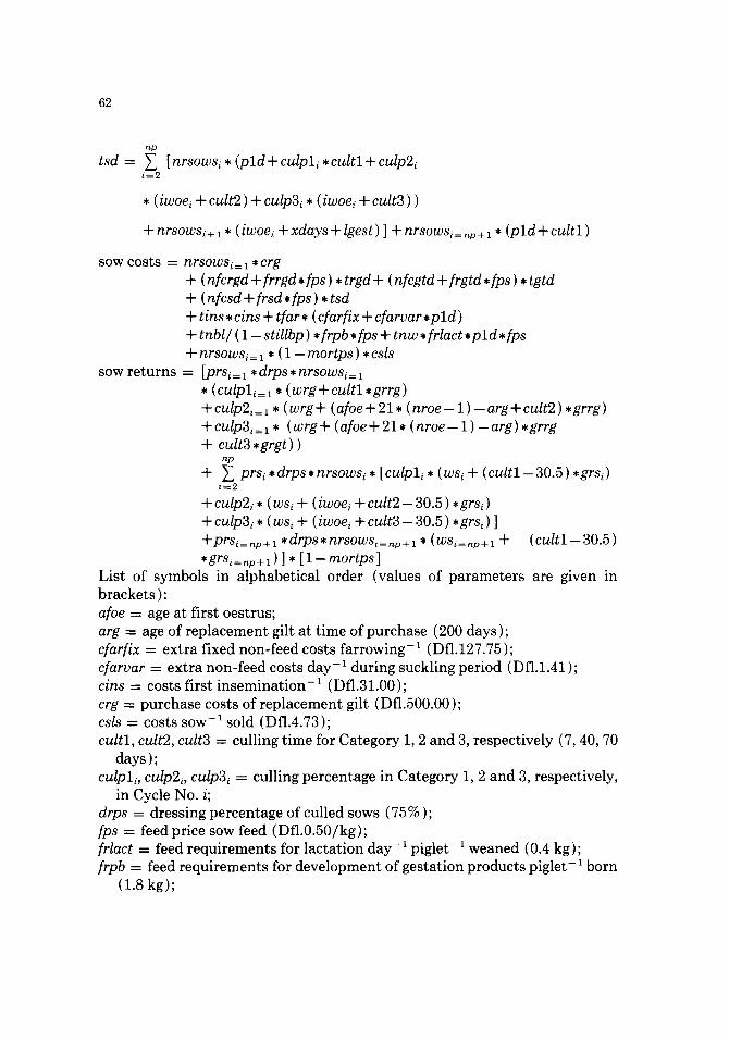
np

tsd = ~ [ nrsowsi * (p l d + culp l i * cu l t l + culp2i i = 2

• (iwoei + cult2 ) + culp3i * (iwoei + cult3 ) )

+ nrsowsi + 1 * ( iwoei + xdays + Igest) ] + nrsowsi = np + 1 * ( p l d + cu l t l )

sow costs = n r s o w s i = 1 * crg + ( n f c r g d + f r r g d , f p s ) , t r g d + ( n f c g t d + f r g t d , f p s ) , t g t d + ( n f c s d + f r s d , f p s ) * t sd + t ins • cins + tfar • (cfarfix + c f a r v a r , p 1 d ) + t n b l / ( 1 - stiUbp ) , f r p b • fps + t n w , [ r l a c t , p l d , f p s + nrsowsi= 1 * (1 - mor tps ) • csls

sow returns = [prsi= 1 * d r p s , nrsowsi= 1 • (culpl i=~ * ( w r g + c u l t l , g r r g ) + culp2i= ~ * ( wrg + ( a l o e + 2 1 , ( nroe - 1 ) - arg + cult2 ) , grrg ) +cu lp3 i= l * ( w r g + ( a l o e + 2 1 , ( n r o e - 1 ) - a r g ) , g r rg + c u l t 3 , g r g t ) )

np

+ ~ prsi * d r p s * n r s o w s i , [ c u l p l i , (wsi + ( c u l t l - 3 0 . 5 ) * g r s i ) i ~ 2

+ culp2i * (wsi + (iwoei + cult2 - 30.5 ) *grsi) + culp3i * ( wsi + ( iwoei + c u l t 3 - 3 0 . 5 ) * grsi ) ] +prsi=n~+~ *drps*nrsowsi=np+~ , (wsi=n~+l + ( c u l t l - 3 0 . 5 ) • g r s i = ~ + l ) ] * [ 1 - m o r t p s ]

List of symbols in alphabetical order (values of parameters are given in brackets): aloe = age at first oestrus; arg = age of replacement gilt at time of purchase (200 days ); cfarfix = extra fixed non-feed costs farrowing- 1 (Df1.127.75); cfarvar = extra non-feed costs day -~ during suckling period (Dfl.l.41); cins = costs first insemination -1 (Dfl.31.00); crg = purchase costs of replacement gilt (Dfl.500.00); csls = costs sow -1 sold (Dfl.4.73); cu l t l , cult2, cult3 = culling time for Category 1, 2 and 3, respectively (7, 40, 70

days ); culpl i , culp2i, culp3i = culling percentage in Category 1, 2 and 3, respectively,

in Cycle No. i; drps -- dressing percentage of culled sows (75%); fps = feed price sow feed (Dfl.0.50/kg); [rlact = feed requirements for lactation day-~ piglet-1 weaned (0.4 kg); ]:rpb = feed requirements for development of gestation products piglet- ~ born

(1.8 kg);

63

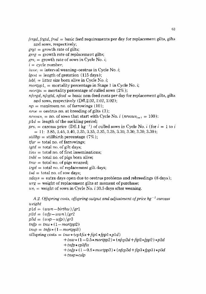
frrgd, frgtd, frsd = basic feed requirements per day for replacement gilts, gilts and sows, respectively;

grgt = growth rate of gilts; grrg = growth rate of replacement gilts; grsi = growth rate of sows in Cycle No. i; i = cycle number; iwoei = interval weaning-oestrus in Cycle No. i; lgest = length of gestation ( 115 days ); lsbli = litter size born alive in Cycle No. i; mortppli = mortali ty percentage in Stage 1 in Cycle No. i; mortps = mortali ty percentage of culled sows (2%); nfcrgd, nfcgtd, nfcsd = basic non-feed costs per day for replacement gilts, gilts

and sows, respectively (Dfl.2.02, 2.02, 2.02); np = maximum no. of farrowings (10); nroe = oestrus no. at breeding of gilts (3); nrsowsi = no. of sows that start with Cycle No. i (nrsowsi=l = 100); p l d = length of the suckling period; prsi = carcass price (Dfl.1 kg -1) of culled sows in Cycle No. i (for i = 1 to i

= 11: 3.85, 3.45, 3.40, 3.35, 3.35, 3.35, 3.35, 3.30, 3.30, 3.30, 3.30); stiUbp = stillbirth percentage (7%); tfar = total no. of farrowings; tgtd = total no. of gilt days; tins = total no. of first inseminations; tnbl = total no. of pigs born alive; tnw = total no. of pigs weaned; trgd -- total no. of replacement gilt days; tsd = total no. of sow days; xdays = extra days open due to oestrus problems and rebreedings (8 days); wrg -= weight of replacement gilts at moment of purchase; ws, = weight of sows in Cycle No. i 30.5 days after weaning.

A,2. weight p l d = p2d -~ p3d = t n f p =

Offspring costs, offspring output and adjus tment of price kg -1 carcass

(wwn- - birthw ) /gr l ( w f p - wwn )/gr2 ( wsp - wfp )/gr3 tnw • ( 1 - mortpp2 )

tnsp = tn fp , ( 1 - mortpp3 ) offspring costs = tnw • (cpl f ix +lip1 , f p p l , p l d )

+ tnw • ( 1 - 0.5 * mortpp2 ) • (nfcp2d +lip2 , fpp2 ) , p 2 d + tnfp • cp3fix + tnfp * ( 1 - 0.5 * mortpp3 ) • (nfcp3d +lip3 , fpp3 ) , p 3 d + tnsp • cslp

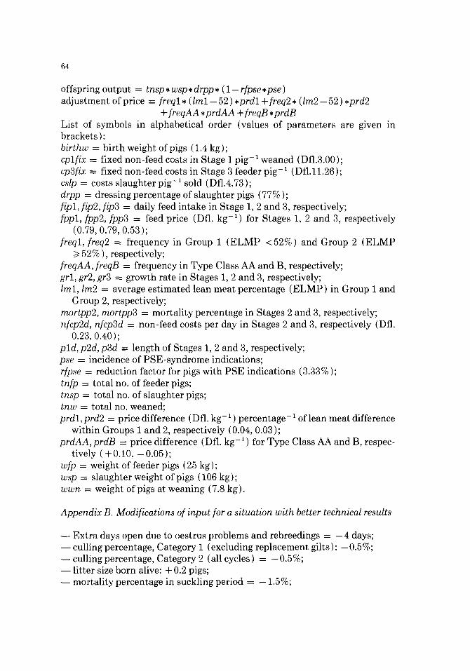
64

offspring output -- tnsp • wsp , drpp , ( 1 - rfpse , pse ) adjustment of price = freql • ( l m l - 52 ) , p r d l + freq2 • ( lm2 - 52 ) , p rd 2

+ f reqAA , p r d A A + freqB , p rdB List of symbols in alphabetical order (values of parameters are given in brackets ): birthw = birth weight of pigs (1.4 kg); cpl f ix = fixed non-feed costs in Stage 1 pig -~ weaned (Dfl.3.00); cp3fix -- fixed non-feed costs in Stage 3 feeder pig -~ (Dfl.ll .26); cslp = costs slaughter pig -1 sold (Dfl.4.73); drpp = dressing percentage of slaughter pigs (77%); lip1, tip2, lip3 = daily feed intake in Stage 1, 2 and 3, respectively; fpp l , fpp2, fpp3 = feed price (Dfl. kg -1 ) for Stages 1, 2 and 3, respectively

(0.79, 0.79, 0.53); [reql, freq2 = frequency in Group 1 (ELMP <52%) and Group 2 (ELMP

>/52% ), respectively; f reqAA, freqB = frequency in Type Class AA and B, respectively; grl , gr2, gr3 = growth rate in Stages 1, 2 and 3, respectively; lml , Ira2 = average estimated lean meat percentage (ELMP) in Group 1 and

Group 2, respectively; mortpp2, mortpp3 = mortality percentage in Stages 2 and 3, respectively; nfcp2d, nfcp3d = non-feed costs per day in Stages 2 and 3, respectively (Dfl.

0.23, 0.40); p l d , p2d, p3d = length of Stages 1, 2 and 3, respectively; pse = incidence of PSE-syndrome indications; rfpse = reduction factor for pigs with PSE indications (3.33%); tnfp = total no. of feeder pigs; tnsp = total no. of slaughter pigs; tnw -- total no. weaned; prd l , prd2 = price difference (Dfl. kg- ~ ) percentage- ~ of lean meat difference

within Groups I and 2, respectively (0.04, 0.03); p r d A A , prdB = price difference (Dfl. kg- ~ ) for Type Class AA and B, respec-

tively (+0.10, -0 .05) ; wfp = weight of feeder pigs (25 kg); wsp = slaughter weight of pigs (106 kg); w w n = weight of pigs at weaning (7.8 kg).

Append ix B. Modif icat ions of input for a s i tuat ion wi th better technical results

- - Extra days open due to oestrus problems and rebreedings = - 4 days; - - culling percentage, Category 1 (excluding replacement gilts): - 0.5%; - -cu l l ing percentage, Category 2 (all cycles) = -0 .5%; w litter size born alive: + 0.2 pigs; - - mortality percentage in suckling period -- - 1.5%;

65

- - g r o w t h r a t e in s u c k l i n g p e r i o d = ÷ 8 g d a y - 1; - - g r o w t h r a t e in n u r s e r y s t a g e -- + 16 g d a y - 1;

- - g r o w t h r a t e in f a t t e n i n g p e r i o d = + 4 5 g d a y - l ;

- - f eed i n t a k e in f a t t e n i n g p e r i o d = ÷ 20 g d a y - 1;

- - m o r t a l i t y p e r c e n t a g e in f a t t e n i n g p e r i o d = - 0 .6%.

REFERENCES

Averdunk, G., Reinhardt, F., Kallweit, E., Henning, M., Scheper, J. and Sack, E., 1983. Compar- ison of various grading devices for pig carcasses. 34th Annual Meeting of the E.A.A.P., Madrid, paper P 6.5, 14 pp.

Brascamp, E.W., 1983. Economic optimization of breeding programs. 3rd International Summer School in Agriculture, Dublin, 59 pp.

C.O.V. (Commissie van Overleg voor de Varkenshouderij), 1976. 44ste Verslag (44th annual report of the Consulting Committee on Pig Production). Commissie van Overleg voor de Var- kenshouderij, Utrecht, 117 pp.

Danell, ().E., 1980. Studies concerning selection objectives in animal breeding. V. Consideration of long and short term effects in defining selection objectives in animal breeding. Thesis, Upps- ala, V: 1-31.

Danell, O. and RSnningen, K., 1981. All-or-none traits in index selection. Z. Tierz. Zuechtungs- biol., 98: 265-284.

Elsen, J.M., Bibe, B., Landais, E. and Ricordeau, G., 1986. Twenty remarks on economic evaluation of selection goals. 3rd World Congress Genetics Applied to Livestock Production, Ne- braska, XII, pp. 321-327.

Gjedrem, R., 1972. A study on the definition of the aggregate genotype in a selection index. Acta Agric. Scand., 22: 11-16.

James, J.W., 1982. Economic aspects of developing breeding objectives: general considerations. In: J.S.F. Barker, K. Hammond and A.E. McClintock {Editors }, Future Developments in the Genetic Improvement of Animals. Academic Press, Sydney, pp. 107-118.

Kanis, E., 1985. Mogelijke consequenties van de nieuwe klassificatie methode voor fokdoel en index. Nota contactcommissie varkensfokkerijonderzoek, 5 pp.

Karlsson, R., 1977. Ekonomiska vikter i svinaveln. Report nr. 18, Uppsala, 75 pp. Knap, P.W., 1986. Selection for fertilty in Dutch pig herdbook breeding. Aggregate genotype,

selection index, and the use of information from relatives. 37th Annual Meeting of the E.A.A.P., Budapest, paper GP 3.12, 16 pp.

Knap, P.W., Huiskes, J.H. and Kanis, E., 1985. Selection index for central test in Dutch pig herdbook breeding from 1984. Livest. Prod. Sci., 12: 85-90.

Ollivier, L., 1986. Economic evaluation of breeding objectives in swine. Introductory remarks. 3rd World Congress Genetics Applied to Livestock Production, Nebraska X, p. xiii.

Ritter, E., Zsorlich, B. and Seyer, D., 1985. Effect of litter size on raising performance until the 95th day of life. Arch. Tierz., 28: 453-463.

Schaaf, A., HerrendSrfer, G. and Ritter, E., 1985. Selektionsmerkmale, Zuchtziele and Zuchtpro- gramme in der Schweinezucht. Arch. Tierz., 28:217-228.

Smith, C., James, J.W. and Brascamp, E.W., 1986. On the derivation of economic weights in livestock improvement. Anim. Prod., 43: 545-551.

Van der Steen, H.A.M., 1986. Genetic and environmental effects on milk consumption and growth during the suckling period in pigs. 3rd World Congress Genetics Applied to Livestock Produc- tion, Nebraska, XI, pp. 234-242.

66

Vangen, O., 1986. Genetic control of reproduction in pigs: from parturition to puberty. 3rd World Congress Genetics Applied to Livestock Production, Nebraska, XI, pp. 169-179.

RESUME

De Vries, A.G., 1989. Un module d'estimation de la valeur dconomique des caract~res utilisds en sdlection porcine. Livest. Prod. Sci., 21: 49 -66 (en anglais).

Un modble d'estimation de la valeur dconomique des caractbres utilisds en sdlection porcine a dtd construit. Ce module ddcrit l'efficacitd de la production de viande comme une fonction des caract~res de l'objectif de sdlection. Les caractbres inclus dans l'objectif de sglection sont: les caractdristiques de roestrus, le poids adulte, les besoins alimentaires et la longdvitd des truies les caractdristiques des port~es, la vitesse de croissance et la consommation journali~re d'aliment des porcelets et des porcs en engraissement, le taux de mortalit~ des porcs, la frdquence de PSE et les caract~res de carcasse.

Le module a dt~ appliqud h la situation nderlandaise. Les valeurs dconomiques {Dfl. par porc abattu) des caract~res les plus importants dtaient: -0 ,09 (par jour) pour l'~ge au premier oestrus, -0,32 (par jour) pour la dur~e de l'intervalle sevrage-oestrus, 8,90 (par porcelet par port , e) pour le nombre de porcelets nds vivants, - 1,10 (par % ) pour le taux de mortalitd des porcelets pendant la pdriode d'allaitement, 2,30 { par raise bas ) pour la longdvitd des truies, 0,26 ( par g par j our) pour la vitesse de croissance des animaux en engraissement, -0,06 ) par g par jour) pour la consommation journali~re des porcs h l'engrais et 3,10 {par % ) pour la teneur en viande maigre.

L'analyse de sensibilitd a montr~ que les valeurs relatives des caract~res pourraient changer dans l'avenir et qu'une rdduction des valeurs absolues est plus vraisemblable qu'une augmentation.

KURZFASSUNG

De Vries, A.C., 1989. Ein Modell zur Schiitzung des 5konomischen Gewichtes von Merkmalen in der Schweinezucht. Livest. Prod. Sci., 21:49-66 (auf englisch).

Es wurde ein Modell zur Sch~itzung des 5konomischen Gewichtes von Merkmalen in der Schweinezucht konstruiert. Das Modell beschreibt die Effizienz der Fleischproduktion als Funk- tion der Merkmale im Zuchtziel. Die Merkmale im Zuchtziel waren: Zyklusmerkmale, Endgewicht und Futterbedarf von Sauen, Nutzungsdauer der Sauen, Wurfmerkmale, Zunahme und t~igliche Futteraufnahme yon Liiufern und Mastschweinen, Verlustrate, PSE-Frequenz und Schlacht- kSrpermerkmale.

Das Modell wurde auf die niederliindische Situation angewendet. Die 5konomischen Gewichte (in niederl~ndischen Gulden pro Schlachtschwein ) der wichtigsten Merkmale waren - 0,09 (pro Tag) ftir das Alter beim ersten ()strus, -0 ,32 (pro Tag) fiir das Intervall Absetzen-0strus, 8,90 (pro Ferkel je Wurf) f'tir die lebend geborenen Ferkel pro Wurf, - 1,10 (pro % ) ftir die Verlustrate yon Saugferkeln, 2,30 (pro Abferkelung) ftir die Nutzungsdauer der Sauen, 0,26 (pro Gramm pro Tag) Rir die Zunahme der Mastschweine, -0 ,06 (pro Gramm pro Tag) Rir die tiigliche Futter- aufnahme der Mastschweine und 3,10 (pro % )fi ir den Fleischanteil.

Eine Sensitivith'tsanalyse zeigte, dai~ sich die relative Bedeutung der Merkmale zuktinftig ver- ~inderen kann und daf~ eine Reduktion der absoluten Werte wahrscheinlicher ist als deren Steigerung.

Documents

A model to estimate economic values of traits in pig breeding