A MODEL OF PRICE DISCRIMINATION UNDER LOSS AVERSION … · A MODEL OF PRICE DISCRIMINATION UNDER LOSS AVERSION AND STATE-CONTINGENT REFERENCE POINTS ... Gabriele Gratton, Paul Heidhues,

A MODEL OF PRICE DISCRIMINATION UNDER LOSS AVERSION

AND STATE-CONTINGENT REFERENCE POINTS

JUAN CARLOS CARBAJAL AND JEFFREY C. ELY

Abstract. We study optimal price discrimination by a monopolist who faces a con-tinuum of consumers with heterogeneous tastes and reference-dependent preferences. Aconsumer’s total valuation for product quality is composed of an intrinsic consumptionvaluation, which is affected by a privately known state signal, and a gain-loss valuationthat depends on deviations of purchased quality from a state-contingent reference qualitylevel. Buyers are loss-averse, so that deviations from their reference levels are evaluateddifferently depending on whether they are gains or losses. As Koszegi and Rabin (2006),we let gains and losses relative to the reference point be evaluated in terms of changesin the consumption valuation, but we differ in terms of how comparisons take place.In particular, because purchasing decisions take place after the state signals have beenobserved, each buyer evaluates consumption outcomes relative to his state-contingentreference quality level. We consider different ways in which reference quality levels areformed, capturing this process by a reference plan, and derive optimal contract menusfor monotone reference consumption plans. The novel effects for product line designdue to the interaction between loss aversion and incomplete information are thoroughlystudied, with special emphasis on self-confirming contract menus, in which the qualitylevels offered by the firm coincides with the reference quality levels. We characterizethe firm’s unique preferred self-confirming contract menu and specify conditions underwhich it also constitutes the consumers’ preferred self-confirming menu.

1. Introduction

Traditionally, the design of the product line has been seen as an attempt from firmsto improve margins by discriminating among consumers with different willingness to pay.In recent years, a growing literature points out various other ways in which contractmenus may affect consumers’ choices. Kamenica (2008) argues that some context effects—e.g., the compromise effect described by Simonson (1989)— can be explained by theinformational content a product line conveys to uninformed buyers: a firm introduces a“premium loss leader” to manipulate consumers’ beliefs about the product characteristicsand increase the demand for less expensive goods. But even in settings where consumershave less problems assessing their intrinsic valuation for a good, context effects may arise ifbuyers care about comparisons between different available options in the product line —asin Orhun (2009)— or comparisons between available options and subjective beliefs aboutconsumption outcomes that act as reference points. In the latter case, the contract menu

Date: October 2013.Key words and phrases. Price discrimination, product line design, loss aversion, reference-dependent

preferences, reference consumption plan, self-confirming contracts.This paper was previously circulated as Optimal contracts for loss-averse consumers. We believe the

new title describes better the contents and message of the paper. We wish to thank Jurgen Eichberger,Gabriele Gratton, Paul Heidhues, Fabian Herweg, Heiko Karle, Jihong Lee, Konrad Mierendorff, LudovicRenou, Antonio Rosato, Klaus M. Schmidt and seminar participants at ANU, CORE, Maastricht Uni-versity, Humboldt University–Berlin, Universities of Zurich, Heidelberg, Munich and New South Wales,NASM–ES 2012, AETW 2012, SITE 2012, and AMES 2013 for helpful comments. Early parts of this workwas conducted while Carbajal was visiting the Department of Economics, University of Bonn; he wishesto thank Benny Moldovanu for his gracious hospitality. Research assistance was provided by AlexandraBratanova and Kim Nguyen. Financial support from the Australian Research Council (Carbajal) and theNational Science Foundation (Ely) is gratefully acknowledged.

1

2 CARBAJAL AND ELY

not only responds to but also shapes those beliefs. This may be in place in the design of aluxury brand product line whose most exclusive items serve as what some commentatorsrefer to as “anchors”. Thus, a premium leader is not introduced to manipulate consumers’beliefs about the product characteristics, but instead to manipulate consumers’ subjectiveexpectations about their own future consumption.1

To help fix some relevant ideas, consider the following hypothetical situation. Anexecutive of an multinational company is planning to buy himself a gift to celebrate asuccessful year before the company announces the next round of senior staff relocation. Hehas decided to spend up to a certain portion of his bonus in expensive personal accessories,and is aware that potential destinations include Chicago and Lima. After spending sometime looking at catalogues, reviews and advertisements, he is convinced that nothing butthe exclusive platinum Grand Complications Patek Philippe watch would be fashionable inChicago, but the less expensive and more practical stainless steel Aquanaut Patek Philippewatch would be appropriate for Lima. By the time he manages to do his shopping,the company has already announced he is to move to Chicago, and therefore his ownexpectations are to purchase the platinum watch. Buying the stainless steel model insteadmay leave a feeling of disappointment, as our executive will compare it with what he wasexpecting to consume in the event of being transferred to Chicago.

The key feature of the above example is the presence of different states that influenceboth consumers’ willingness to pay for a certain good and their subjective expectationsof future consumption. A reasonable conjecture is that these expectations can be manip-ulated, to some degree, by the design of the product line, and firms may find profitable todo so when consumers compare their actual purchasing decisions with their expected con-sumption levels. How shall a firm specify its optimal contract menu under these circum-stances? To investigate these issues, we propose a model of monopoly price discriminationwhen consumers’ preferences are heterogeneous and exhibit loss aversion. In our model,presented in Section 2, there is a state parameter, lying in an interval of the real line, thataffects both consumers taste for quality and their expectations of future consumption.2

To be more precise, we assume that a consumer’s purchasing decision is determined byhis intrinsic taste for product quality and, in addition, by comparisons between the of-fered quality level and a reference quality level. Moreover, both the willingness to pay forquality and the reference quality level are determined by the realization of the state pa-rameter θ, which we also refer to as the consumer’s type. Thus, after observing his type,a potential customer enters the market anticipating a certain reference consumption leveland experiences gains or losses relative to his state-specific consumption utility accord-ing to whether his chosen quality exceeds or falls short of the state-contingent referencepoint. The monopolist’s optimal product line design takes consumers’ reference depen-dence into account and reflects the interaction between loss aversion and the traditionalrent extraction and incentive compatibility tradeoff.

The way we allow the state parameter to determine willingness to pay for quality isstandard (so, for instance, the single-crossing condition is satisfied). To model the inter-action between the state parameter and the reference point, we assume the existence of areference plan; i.e., a weakly monotone increasing function mapping types into referencequality levels. This way, a higher type signifies a higher willingness to pay and a higher

1Christina Binkley, reporting for The Wall Street Journal (The Psychology of the $14,000 Handbag,August 9, 2007), quotes “retail-consulting guru Paco Underhill” explaining how this strategy dates backto the 17th century: “You sold one thing to the king, but everyone in court had to have a lesser one.”2Our model builds on classic monopoly pricing models under asymmetric information developed by Mussaand Rosen (1978) and Maskin and Riley (1984).

PRICE DISCRIMINATION UNDER LOSS AVERSION 3

reference quality level.3 We then derive the optimal contract menu for any such refer-ence plan. Our approach enables comparative statics analysis of the offered product lineas well as monopoly profits arising from changes in the level and shape of the referenceplan, for example due to targeted advertising, fashion and product shows, and so forth.Importantly, we assume that consumers can always shun the firm’s offers and opt insteadto buy an inexpensive substitute good of minimal quality in a secondary market: if ourexecutive is relocated to Lima and, despite his expectations, decides against the $14,000stainless steel watch, he nonetheless purchases the $500 knockoff. Why would a consumerfeel a loss when he opts for the outside option? Because the realization of a particularstate, and the consequent anticipation of consumption, creates what Ariely and Simonson(2003) called a “pseudo-endowment effect”.

In Section 3 we analyze the benchmark model in which the realization of the stateparameter is observed by the monopolist. We show how loss aversion invites upwarddistortions in the offered quality levels relative to the loss-neutral complete informationcase. This occurs, in particular, when buyers enter the market with high reference qualitylevels. In this case, the first-best quality would fall short of the reference level and the loss-averse consumer is willing to pay a premium to reduce the associated loss. The monopolistexploits this by increasing both quality and price until either these marginal gains areexhausted or the offered quality hits the reference level, shutting down any further gains.In particular, over a wide range of states, profit maximization implies matching referencequalities exactly. A similar logic drives the comparative statics results under completeinformation. If the monopolist is able, say via advertising or from historical productofferings, to inflate consumers’ reference levels, then the effect would magnify upwarddistortions in the product line and increase revenue. While an empirical demonstration ofinefficiently high quality offers by firms may be challenging,4 our predictions here couldbe used to indirectly test for loss aversion in the laboratory: everything equal, loss-averse consumers will respond to higher reference consumption points differently thanloss-neutral consumers.5

In Section 4 we turn to our full model in which the realization of the state parameter isprivately known to each consumer and unobservable by the monopolist. A contract menuis now feasible only if it satisfies the self-selection incentive compatibility and participationconstraints. We study the novel ways in which these constraints interact with consumptionloss aversion. Two new effects emerge, compared to the complete information benchmark.First, the marginal profitability of increased quality is reduced due to incentive issuesfamiliar from traditional models of monopoly price discrimination. Higher quality levelsare more attractive to a θ-consumer with low willingness to pay, but also more attractiveto consumers with more favorable state signals, to whom the monopolist was hoping tosell an even higher quality product. The increase in revenues from the θ-consumer will beoffset by information rents ceded to these consumers, to discourage them from choosing thequality product designed for the θ-consumer. Reference dependence enters, and modifiesthis standard tradeoff because the higher taste for quality implies that for any given qualityand reference levels, the higher type consumer experiences a larger loss (or smaller gain)

3Monotonicity on the reference plan restricts how wrong buyers are allowed to be: a consumer with alow state signal, and consequently low intrinsic valuation, may expect to buy as much quality as, but notmore than, a consumer with a high state signal.4Yet it is hard to justify, purely in terms of welfare considerations, products like the mechanical stopwatch Carrera Mikrograph Chronograph offered by Tag Heuer, which measures time at the 1/100thsecond precision.5These predictions are consistent with the findings reported by Heyman, Orhun, and Ariely (2004),who tested the pseudo-endownment effect in experimental auctions to explain multiple bidding in onlineauctions. One explanation they advanced is that the anticipation of ownership increases the valuation ofthe object from its initial level.

4 CARBAJAL AND ELY

than the θ-consumer. Thus, it is possible for the firm to increase profits by expanding itsproduct line to both high and low ends of the market, in response to (or in anticipationof) consumers’ high expectations.6 This loss aversion effect can also account for threepart tariffs and other complex contract schemes that have become increasingly popularamong mobile phone operators, Internet providers, and other subscription services,7 whenfor instance, low type consumers overestimate usage prior to choosing a contract.

The second effect is a novel distortion due entirely to loss aversion and has no coun-terpart in loss-neutral screening model. Consider a monopolist contemplating increasingthe quality q offered to a given θ-consumer from just below his state-contingent referencelevel to just above it. Such a change has a discrete effect on the attractiveness of q toconsumers who received higher signals, thus have higher willingness to pay, but whosereference levels are relatively similar. As a result, the monopolist would incur a discretedrop in profits due to information rents, were it to boost quality levels above the referencepoint of the θ-consumer. We quantify this lump-sum incentive cost and show its effectson the optimal product line and comparative statics. It implies an additional downwarddistortion in quality levels to consumers who would otherwise be offered products thatsurpass their reference points. It also implies that increased reference qualities may ac-tually decrease offered qualities, so the interaction between reference quality levels andoffered qualities under loss aversion and incomplete information is quite complex. Finally,it impacts the profitability of shaping reference points through, for example, advertisingcampaigns. Parallel shifts upward in reference plans always increase profits, but changesin the shape of the reference plan can have ambiguous effects. We illustrate these issuesin a simple example with uniform signals, linear valuations, and quadratic cost.

The fact that the reference plan determines to a great extent qualitative features of theoptimal product line leads to the question of belief manipulation, both on the part of thefirm and on the part of the consumers. This issue is explored in Section 5, where we imposea consistency requirement on admissible reference plans. Specifically, we focus on self-confirming reference consumption plans; i.e., subjective beliefs about future consumptionoutcomes that coincide, in equilibrium, with the actual outcomes. Thus, our model allowsus to analyze the consequences of reference plans as correct endogenous beliefs in optimalproduct line design. We find that, while the set of optimal self-confirming contracts isstrictly smaller than the set of optimal contracts, it nonetheless contains quality scheduleswith most of the features described in the previous paragraphs. On the other hand, it issurprisingly simple to show that there exists a unique self-confirming contract menu thatis preferred by the firm. Indeed, in any given self-confirming product line, each consumerbuys his state-contingent reference quality level. Since a higher reference plan weaklyincreases the net total willingness to pay, as it makes the external, minimal quality optionless desirable (due, again, to the pseudo-endowment effect), it follows that profits areincreasing in the reference plan. Thus, the preferred self-confirming product line for thefirm usually excludes fewer consumers from the market and has quality levels distortedupward from second best levels under loss neutrality to the levels that maximize netvirtual surplus for loss-averse consumers. While these upward quality distortions improveallocative efficiency for low and intermediate type consumers, buyers with high stateparameters end up purchasing overly sophisticated goods.

In practice, firms can manipulate reference points through advertising and other mar-keting practices prior to the introduction of the product line into the market.8 Marketing

6So, in addition to overly sophisticated and exclusive items, luxury brand product lines include minoraccessories: keychains, bookmarks, and phone straps.7See for example Lambrecht and Skiera (2006) and Lambrecht, Seim, and Skiera (2007).8Product shows in anticipation of market entrance are standard practice in, among others, the luxurygoods, cars, and consumer electronics industries.


efforts will be credible as long as they promote optimal self-confirming product lines. Ahigher self-confirming reference plan never decreases the firm’s expected profits or offeredqualities, but it may or may not hurt consumer’s surplus —note we are comparing howdifferent self-confirming reference plans affect loss averse consumers. This is because ahigher reference quality plan implies higher quality offers for (potentially more) activeconsumers, which translates into more information rents assigned to buyers with posi-tive consumption levels. Yet, higher reference quality levels may be detrimental because,by diminishing the value of the outside option, they increase the net willingness to payof active consumers.9 We specify conditions under which the positive information rentseffect associated with a higher self-confirming reference plan dominates the negative par-ticipation effect. In this case, the firm’s preferred self-confirming contract menu is alsothe consumer’s preferred contract menu. This result relies on two assumptions. First, ahigher state parameter implies higher marginal intrinsic consumption valuation for qualitydue to single-crossing, but these effects are diminishing in the quality dimension. Sec-ond, consumers have quasi-linear utilities for the good offered by the firm and face nobudgetary restrictions.

Section 6 offers some concluding remarks. Omitted proofs from the text are gatheredin Section 7.

Related literature

Our work contributes to the line of inquiry pioneered by DellaVigna and Malmendier(2004), Eliaz and Spiegler (2006), and Heidhues and Koszegi (2008), among others, thatinvestigates how profit maximizing firms operate in a market context where consumershave systematic deviations from traditional preferences. Galperti (2011) and Grubb(2009) are additional recent contributions.

Following Koszegi and Rabin (2006), we model the consumer’s gain-loss valuation interms of differences in the consumption valuation. Importantly, we differ in how compar-isons take place. In some economic contexts it is reasonable to assume, as Koszegi andRabin (2006) and Heidhues and Koszegi (2012), that all buyers share an ex ante stochasticreference point and evaluate each realization of stochastic consumption with each poten-tial realization of the reference point. However, in other situations —for instance, whenheterogeneous consumers face a discriminating monopolist and make purchasing decisionsat the interim stage— it may be more appropriate to let each buyer assess his quality con-sumption relative to his state-contingent reference quality level, and this is the approachwe follow here. Our work in this respect is closer to Sugden (2003); see also De Giorgiand Post (2011). Recent papers that follow Koszegi and Rabin’s (2006) approach includeRosato (2013), who studies how bait-and-switch tactics manipulate reference points andraise profits even when consumers rationally expect the bait and switch; Hahn, Kim, Kim,and Lee (2012), who study non-linear pricing when consumers form reference points at anex ante stage before learning their valuation but anticipating the eventual type-dependentconsumption (thus consumers have a type-independent stochastic reference point); andEisenhuth (2012), who looks at the optimal auction for bidders with expectations-basedreference points —see also Lange and Ratan (2010).

Our work is related to Orhun (2009), who considers a two-type model in which thereference point of the high-type consumer is influenced by the quality offered to the low-type consumer and vice versa. We consider optimal product line design in response toan arbitrary, and fixed, reference plan. This enables us to study the incentives of themonopolist to manipulate reference points, perhaps via advertising. Karle (2013) studiesadvertising to loss-averse consumers using a model of expectations-based reference pointformation with stochastic consumption a la Koszegi and Rabin (2006). In his model,

9We thank an anonymous referee for pointing out this effect, which was previously omitted from ouranalysis.

6 CARBAJAL AND ELY

advertising creates uncertainty about future consumption and this impacts reference pointformation, whereas the logic of our model indicates that the firm will try to drive up eachconsumer’s reference quality level unambiguously.

Throughout this paper, we model reference points in terms of quality levels, departingfrom recent work in the area such as Herweg and Mierendorff (2013) and Spiegler (2011),that specifies reference points in terms of prices. Despite the evidence supporting theexistence of reference price effects on consumer behavior, empirical work from the mar-keting literature suggests that loss aversion on product quality is at least as importantas, if not more important than, loss aversion in prices.10 This point is also suggestedby experimental data reported by Fogel, Lovallo, and Caringal (2004), who confirm theexistence of loss aversion for quality in a laboratory setting, and Novemsky and Kahne-man (2005), who stress that there is no loss aversion for monetary transactions that areexpected to occur and thus accounted for (in the sense of Thaler (1985), for instance). Inour setting —as in the motivating example— consumers are not subject to meaningfulbudgetary restrictions, so we treat potential expenses on the good in question as part ofa budget established for transaction purposes. Thus, price differences among goods ofvarious qualities are evaluated solely in terms of willingness to pay and do not registerneither as gains nor as losses.

2. Product Line Design under Reference-Dependent Preferences

In this section we lay out the notation and main assumptions of our model, whichbuilds on work by Mussa and Rosen (1978) and Maskin and Riley (1984), among oth-ers. In our framework, a consumer derives utility from consumption and, in addition,from comparisons between actual consumption and a state-contingent reference point.Following Tversky and Kahneman (1991), we consider loss-averse consumers.

2.1. The firm. A revenue-maximizing monopolist produces a good of different charac-teristics captured by the product attribute parameter q ≥ 0. This parameter can beinterpreted as either a one-dimensional measure of quality (exclusive features in a luxuryproduct line) or quantity (amount of data offered by a mobile operator). We follow Mussaand Rosen (1978) and maintain the first interpretation, thus referring to q as the qualityattribute.

The cost of producing one unit of the good with quality q is represented by c(q),where the cost function q 7→ c(q) is non-decreasing, twice continuously differentiable, andsatisfies c(0) = 0. In addition, we assume that there exists a positive number ε suchthat cqq(q) ≥ ε > 0 for all quality levels.11 The firm’s problem is to design a revenuemaximizing product line (i.e., a contract menu of posted quality–price pairs) to offer topotential buyers with differentiated demands.

2.2. Consumers. There is a population of consumers with quasi-linear preferences andunit demands for the good offered by the firm, but heterogeneous tastes for the productattribute. Preference heterogeneity depends on a state parameter (type) θ ∈ Θ = [θL, θH ],where 0 < θL < θH < +∞. The realization of the state signal is private information, sothat the firm only knows the distribution F , with full support on Θ and density f > 0.We assume that the inverse hazard rate θ 7→ h(θ) ≡ (1 − F (θ))/f(θ) is non-increasingand twice continuously differentiable.

10See Hardie, Johnson, and Fader (1993) for instance. Bell and Lattin (2000) suggest that accountingfor heterogeneity in consumers’ price response significantly lowers previous estimates of the loss aversionprice-coefficient. Their work does not consider estimates for loss aversion in product attributes.11Throughout the paper we use subindices to denote (partial) derivatives. Therefore cqq positive andbounded away from zero means that the cost function is strongly convex.


A θ-consumer has a consumption valuation for quality q ≥ 0 given by m(q, θ). Toavoid any complication arising from the classical screening framework, we impose thefollowing regularity assumptions: (a) (q, θ) 7→ m(q, θ) is twice continuously differentiable;(b) for every θ ∈ Θ, the function q 7→ m(q, θ) is strictly increasing and concave, withm(0, θ) = 0; (c) for every quality level q ≥ 0, the function θ 7→ m(q, θ) is non-decreasing,with mθ(0, θ) = 0; (d) for all pairs (q, θ), mqθ(q, θ) > 0, so that the single-crossingcondition holds. In addition, we assume that for all types θ the following holds:

limq→0

(mq(q, θ)− cq(q)) > 0 and limq→+∞

(mq(q, θ)− cq(q)) < 0.

This specification includes, among others, Mussa and Rosen’s (1978) monopoly modelwith linear consumption valuation and quadratic costs. It ensures that the quality sched-ule that maximizes consumption surplus is continuously differentiable on Θ and non-decreasing in types. An alternative to accommodate Maskin and Riley’s (1984) model isto impose strong concavity of m and convexity of c.

We step aside from standard monopoly pricing theory and consider buyers who exhibitreference-dependent preferences for the product attribute (but not its price). Specifically,we assume that in addition to his consumption valuation, a θ-consumer derives utilityfrom comparing quality q to a type-contingent reference quality level r(θ). A referencequality level may encompass different concepts: it can reflect (in)correct subjective ex-pectations of future consumption; it may be determined by past experiences or by currentaspirational considerations, etc. At this stage, it is convenient to study a general referenceformation process, which we capture by the reference consumption plan θ 7→ r(θ) ≥ 0. Weassume that this reference plan is non-decreasing, continuous and piecewise continuouslydifferentiable, with bounded left and right derivatives for all state signals θ ∈ Θ.

Following Koszegi and Rabin (2006), we let comparisons between consumption out-comes and reference points be evaluated in terms of changes in the consumption valuation.On the other hand, we assume that each buyer assesses quality consumption relative tohis own state-contingent reference quality level. Thus, after observing state parameterθ, a consumer has a gain-loss valuation for q given by µ × (m(q, θ) −m(r(θ), θ)), whereµ = η if q > r(θ) and µ = ηλ if q ≤ r(θ). The parameter η > 0 is the weight attached tothe gain-loss valuation and the parameter λ ≥ 1 is the loss aversion coefficient. We treatthe loss neutrality case (i.e., λ = 1) as a baseline scenario. The total valuation for theθ-consumer derived from purchasing one unit of the good with quality q ≥ 0 is then:

m(q, θ) + µ×(m(q, θ) − m(r(θ), θ)

).

Since preferences are quasi-linear, the utility that the θ-consumer obtains from buyinga good with quality q at price p is his total valuation minus the price. The value of theoutside option for a buyer, if he chooses not to trade with the firm, is taken to be thepayoff derived from purchasing a minimal quality substitute good in a secondary market.For simplicity, we let both quality and price of the substitute good be equal to zero. Thismeans that the θ-consumer’s utility from the outside option is −ηλm(r(θ), θ), and hebuys from the firm only if his utility is no less than this value. The net total valuation ofthe θ-consumer from purchasing a good of quality q is then:

v(q, θ) ≡ (1 + µ)m(q, θ) + (ηλ− µ)m(r(θ), θ), (1)

where, as before, µ = η if q > r(θ) and µ = ηλ if q ≤ r(θ). Presented with a contractto purchase quality q at price p, a θ-consumer with reference quality level r(θ) choosesto do so as long as his net total utility v(q, θ) − p is non-negative. This constitutes the(endogenous) participation constraint.

8 CARBAJAL AND ELY

2.3. Comment. We provide the following interpretation of our framework. There is amass of ex ante identical consumers interacting with the firm on a given time period. Priorto entering the market, consumers have a common reference consumption plan, based oncorrect or incorrect subjective beliefs or other aspirational considerations about futureconsumption outcomes. Later, each consumer receives a state parameter that affects hiswillingness to pay for the product attribute and, in addition, fixes his reference qualitylevel according to the reference plan. The firm knows the distribution of state signals butdoes not observe their realizations. Thus, the firm designs a menu of individually rationaland incentive compatible posted contracts to maximize expected revenue. Once contractsare posted, each θ-consumer evaluates a quality level in any given contract relative tohis state-contingent reference quality level r(θ). The consumer then purchases his mostpreferred contract from the firm as long as the net total utility derived from this selectionis non-negative.

Throughout the paper, we assume that the consumption valuation, the gain-loss valu-ation and the reference plan are common knowledge. That is, the firm is fully aware ofthe consumers’ behavioral bias. We take a partial equilibrium approach and ignore anybudgetary restriction on consumer’s behavior. Insofar as the total willingness to pay ofloss-averse consumers for a given level of product quality is influenced by the referenceplan, we focus on allocative efficiency alone when discussing welfare implications of lossaversion, taking loss neutrality as a baseline scenario from which to compare effects ofreference-dependent preferences, so that we can highlight the effects of loss aversion.

3. Price Discrimination under Complete Information

We begin by analyzing optimal product line design under complete information. Fixinga reference plan θ 7→ r(θ), when types are observable the firm cannot do better thancharging the θ-consumer the whole of his net total valuation and earn (per customer)profits equal to (per customer) total surplus

TS(q, θ) ≡ (1 + µ)m(q, θ) + (ηλ− µ)m(r(θ), θ) − c(q). (2)

The firm’s profits are therefore maximized by offering the θ-consumer a quality level thatmaximizes total surplus:

qfb(θ) = arg maxq≥0

TS(q, θ).

Observe that total surplus depends directly and indirectly on the quality level, as theposition of q relative to the reference level r(θ) determines the value that µ adopts inEquation 2. To find the solution to the firm’s problem, define

S(q, θ;µ) ≡ (1 + µ)m(q, θ) − c(q)

as the part of total surplus from the θ-consumer directly affected by the choice of quality,for each µ ∈ {η, ηλ}, and the quality schedule θ 7→ q(θ;µ) as the mapping

q(θ;µ) = arg maxq≥0

S(q, θ;µ), for µ = η, ηλ.

By our assumptions, q(·;µ) is continuously differentiable and non-decreasing.12 In par-ticular, since the consumption valuation is strictly increasing in q, we have 0 < q(θ; η) <q(θ; ηλ) for all state signals θ ∈ Θ.

Note that under loss neutrality (λ = 1), the net total valuation is independent of thereference quality level. From Equation 2, total surplus in this case is given by

TS(q, θ) = S(q, θ; η),

12Recall that, for each θ, the consumption valuation is twice continuously differentiable and concave in q,and the cost function is strongly convex.


and thus the first-best monopoly qualities are qfb(θ) = q(θ; η), independently of r(θ). Wetherefore interpret q(θ; η) as the classic efficient (i.e., surplus maximizing) quality levelunder loss neutrality.

The solution of the monopolist problem under loss aversion (λ > 1) is now easilyobtained by noticing that TS(·, θ) coincides with S(·, θ; ηλ) when q is less than or equal tor(θ), and with a constant-shifted loss-neutral surplus S(·, θ; η) whenever q is greater thanr(θ). Since S(·, θ; η) has a strictly smaller slope than S(·, θ; ηλ), the total surplus functionexhibits a kink at q = r(θ). The quality level that maximizes profits is determined bythe location of the kink relative to the two maximizers q(θ; η) and q(θ; ηλ). Refer toFigure 1 for an illustration. If the reference quality level r(θ) is below q(θ; η), then profitsare increasing at the kink point and the firm chooses the efficient quality level q(θ; η)—Figure 1(A). Similarly, if r(θ) lies above q(θ; ηλ), then profits are decreasing at the kinkpoint and the firm sets quality at the latter level —Figure 1(B). If the reference pointr(θ) lies in intermediate ranges, any deviation from the reference quality level will hurtprofits and the optimal quality level is therefore r(θ) —Figure 1(C).

This leads to the following observation.

Proposition 1. Given a reference plan θ 7→ r(θ), the complete information contract menudesigned by the monopolist for loss-averse consumers consists of quality–price schedulesθ 7→ (qfb(θ), pfb(θ)) such that:

qfb(θ) =

q(θ; ηλ) : r(θ) ≥ q(θ; ηλ),

r(θ) : q(θ; ηλ) > r(θ) > q(θ; η),

q(θ; η) : q(θ; η) ≥ r(θ);

andpfb(θ) = (1 + µ)m(qfb(θ), θ) + (ηλ− µ)m(r(θ), θ),

where µ = η whenever qfb(θ) > r(θ) and µ = ηλ otherwise.

Proposition 1 shows the effects of reference-dependent preferences and loss aversionon price discrimination in the absence of screening issues. For a low reference level, thefirm’s optimal quality will be in the domain of gains and therefore coincides with theloss-neutral case. When the reference quality at state θ exceeds the q(θ; ηλ) threshold,the optimal quality must be in the domain of losses and the firm exploits consumer’s lossaversion by increasing its offer from the classic efficient level to q(θ; ηλ). Note that thereference plan entirely determines the shape of first-best quality offers for consumers withintermediate reference levels, that is when q(θ; η) ≤ r(θ) ≤ q(θ; ηλ). Since the referenceconsumption plan may in principle be very general, first-best contracts can take variousshapes. In particular, there may be pooling among certain consumer segments due to acommon reference quality level.

We can understand these results better if we consider the comparative statics effect onfirm profits and offered qualities of an increase in the reference level. These comparativestatics are also of independent interest as they inform extensions of the model that wouldenable the firm to manipulate the reference level. The key observation is that a change inthe reference level affects how the consumer evaluates not only the contracted quality butalso the outside option —this is similar to the pseudo-endowment effect noticed by Arielyand Simonson (2003). In particular, if marketing increases the consumer’s anticipatedquality, then it also reduces the attractiveness of the outside option, further binding theconsumer to the contract.

Suppose that r(θ) < q(θ; η), so that the reference quality lies strictly between theoutside option (i.e. the zero quality good sold in the secondary market) and the optimalquality offered by the firm. The consumer is comparing his outside option in the domain oflosses with the firm’s offer in the domain of gains. An increase in r(θ) has countervailing

10 CARBAJAL AND ELY

TS ( · , θ)

q(θ; ηλ)q(θ; η)r (θ)

(a) qfb(θ) = q(θ; η)

q(θ; η) q(θ; ηλ)

µ = ηµ = ηλ

TS ( · , θ)

r (θ)

(b) qfb(θ) = q(θ; ηλ)

TS ( · , θ)

q(θ; η) q(θ; ηλ)

µ = ηλ

µ = η

r (θ)

(c) qfb(θ) = r(θ)

Figure 1. Total surplus function TS(·, θ): the optimal quality is deter-mined by the position of the kink.

effects: it increases the loss associated with the outside option but reduces the gainassociated with the contract. Because marginal losses weigh more heavily than gains underloss aversion, the net effect increases the relative attractiveness of the firm’s contract. Thefirm’s quality offer is unchanged, but the consumer’s willingness to pay, hence the firm’sprice, increases by

(ηλ− η)mq(r(θ), θ).

As soon as reference qualities exceed the loss-neutral efficiency level q(·; η), both thequality and the outside option will be in the domain of losses and any further increasein the reference quality reduces the value of both equally, leaving the consumer’s netvaluation unchanged. However, the firm may now profitably increase quality above loss-neutral efficient levels. In particular, since offered qualities will be in the domain of losseswhere total surplus rises more steeply, there are larger surplus gains from quality. Thefirm will capture these gains by increasing quality up to the reference level where the netvaluation and total surplus exhibit kinks. This increases profits by

(1 + ηλ)mq(r(θ), θ) − cq(q).

Finally, once the reference quality r(θ) exceeds q(θ; ηλ), all gains from loss aversion havebeen exhausted and the firm’s offered quality and price are unaffected by further increasesin reference levels.

We stress that the ability to exploit a higher reference plan and distort qualities aboveand beyond efficiency levels depends on loss aversion: when consumers are loss-neutral, theoptimal product line is independent of the reference consumption plan. These observationsare gathered in the next result.

Proposition 2. The following holds under complete information. For loss-neutral con-sumers:


1. Optimal qualities offered by the firm coincide with classic efficient qualities, qfb(θ) =q(θ; η), regardless of the reference consumption plan.

For loss-averse consumers:

2. Optimal qualities offered by the firm are weakly greater than the loss-neutral effi-cient levels, and strictly greater when r(θ) > q(θ; η).

3. An increase in the reference quality level weakly increases the firm’s profits, andstrictly increases profits whenever r(θ) ≤ q(θ; ηλ).

4. An increase in the reference quality level weakly increases the offered quality bythe firm, and the increase is strict whenever q(θ; η) ≤ r(θ) ≤ q(θ; ηλ).

4. Price Discrimination under Incomplete Information

In this section we study optimal product line design for a monopolist facing loss-averseconsumers, when the realization of the state parameter is private information and themonopolist only knows the distribution F and the support Θ.

4.1. The design problem. Fixing a reference plan θ 7→ r(θ), the problem of the firmcan be formally stated as follows. Choose a menu of posted quality–price contracts θ 7→(q(θ), p(θ)) that maximizes expected profits

Πsb =

∫ θH

θL

{p(θ) − c(q(θ))

}f(θ) dθ

subject to the incentive compatibility constraints:

v(q(θ), θ) − p(θ) ≥ v(q(θ′), θ) − p(θ′), for all θ, θ′ ∈ Θ; (3)

and the individual rationality constraints:

v(q(θ), θ) − p(θ) ≥ 0, for all θ ∈ Θ. (4)

A menu of contracts that satisfies both informational constraints is said to be incentivefeasible. When there is no risk of confusion, we let

U(θ) = v(q(θ), θ) − p(θ)

denote the indirect utility function associated with an incentive feasible product line.Notice that the value the gain-loss coefficient µ implicitly takes in each side of the incen-

tive compatibility inequality Equation 3 may differ, as it depends on comparison of q(θ)with r(θ) on the left-hand side, and comparison of the alternative offer q(θ′) with r(θ) onthe right-hand side. Suppose for a moment that the reference plan is strictly increasing.If r(θ) coincides with the quality offered to the θ-consumer, then the gain-loss coefficientwill change abruptly depending on whether the bundle for the θ-consumer is selected by alower type consumer, who experiences a gain with respect to his personal reference level,or a higher type consumer, who experiences a loss relative to his also higher referencequality level. This sudden change in the net total valuation due to the presence of lossaversion complicates the application of standard contract theoretic techniques, based onthe usual integral representation of incentive compatibility, to characterize incentive feasi-ble contracts when the monopolist faces a continuum of consumers.13 Figure 2 illustratesthe source of the problem.

Given an incentive feasible menu of contracts, U(θ) represents the maximum utility theθ-consumer can obtain among all of the available options. Therefore, when we considerany particular contract (q(θ′), p(θ′)) and plot the utility

θ 7→ v(q(θ′), θ) − p(θ′),

13As proposed by Mussa and Rosen (1978) and Myerson (1981), and more recently by Williams (1999),Krishna and Maenner (2001), Milgrom and Segal (2002), among others.

12 CARBAJAL AND ELY

U ( ·)

θ θ = q− 1 ( r ( θ))

(a) Determinacy

U ( ·)

θ = q− 1 ( r (θ ))

(b) Indeterminacy

Figure 2. Kinks cause standard techniques based on the envelope theo-rem to fail.

the indirect utility function θ 7→ U(θ) must lie everywhere above it, and coincide withit at θ = θ′. When, as in Figure 2(A), v(q(θ′), ·) is differentiable at θ′, this pins downthe derivative of the indirect utility, and if this is true for almost every θ-consumer, thenthese derivatives can be integrated to recover U(θ).14 However, when the quality q(θ′)allocated to the θ′-consumer coincides with the reference quality r(θ′), then the mappingv(q(θ′), ·) exhibits a kink at the point θ = θ′ and this can lead to an indeterminacy, asillustrated in Figure 2(B).15

On the other hand, for all q ≥ 0, the total valuation has bounded left and right partialderivatives for every type θ ∈ Θ, which we denote respectively by v−θ (q, θ) and v+θ (q, θ).One conjecture is that it is possible to use the left or the right derivative of the totalvaluation in place of its derivative, when this last does not exist, to express the indirectutility under an incentive feasible contract menu, and thus to express expected profits interms of virtual surplus. To show a more general result, let us define the correspondenceθ ⇒ ϕ(q, θ) associated with quality level q as

ϕ(q, θ) ≡{δ ∈ R | v+θ (q, θ) ≤ δ ≤ v−θ (q, θ)

}.

When the reference quality level for the θ-consumer does not coincide with q, the nettotal valuation has a partial derivative with respect to types, so that ϕ(q, θ) = vθ(q, θ).When r(θ) = q and the reference plan is strictly increasing at θ, because of loss aversion,the right derivative of the total valuation is strictly smaller than its left counterpart, henceϕ(q, θ) will be a closed, bounded interval. One readily obtains the following expressionfor each θ-consumer (see Section 7 for details):

ϕ(q, θ) =(1 + ηλ)mθ(q, θ) : r(θ) > q,

(1 + η)mθ(q, θ) + (ηλ− η) ddθ(m(r(θ), θ)

): r(θ) < q,[

(1 + ηλ)mθ(q, θ) , (1 + η)mθ(q, θ) + (ηλ− η) ddθ(m(r(θ), θ)

)]: q = r(θ).

(5)

We stress that since product quality is a choice variable of the firm, it could be optimalto offer contracts such that q(θ) = r(θ) for a subset of consumers of positive measure. Iffor these buyers the reference plan is strictly increasing, it follows that in equilibrium thetotal valuation may fail to be differentiable in types, and therefore our correspondence inEquation 5 will be multi-valued, on a non-negligible subset of consumers in Θ. In this case,

14This statement is simply the envelope theorem.15The reference plan is piecewise continuously differentiable, hence we omit discussion of kinks in thetotal valuation due to kinks in the reference plan. This is inconsequential for the derivation of the optimalproduct line.


we characterize incentive feasible contracts based on an integral monotonicity conditionand a generalization of the Mirrlees representation of the indirect utility.16 Given a(measurable) quality schedule θ 7→ q(θ), its associated correspondence θ ⇒ ϕ(q(θ), θ)derived using Equation 5 is non empty-valued, closed-valued, bounded and measurable.Thus, it admits integrable selections. We use the notation θ 7→ δ(q(θ), θ) ∈ ϕ(q(θ), θ) toindicate an integrable selection. The following proposition provides a characterization ofthe incentive feasible product line offered by the monopolist.

Proposition 3. Under incomplete information, the product line θ 7→ (q(θ), p(θ)) designedby the firm for loss-averse consumers is incentive feasible, with associated indirect utilityU(θ) = v(q(θ), θ) − p(θ), if and only if there exists an integrable selection θ 7→ δ(q(θ), θ)of the correspondence θ ⇒ ϕ(q(θ), θ) for which the following conditions are satisfied.

(a) Integral monotonicity: for all θ′, θ′′ ∈ Θ,

v(q(θ′′), θ′′) − v(q(θ′′), θ′) ≥∫ θ′′

θ′δ(q(θ), θ) dθ ≥ v(q(θ′), θ′′) − v(q(θ′), θ′).

(b) Generalized Mirrlees representation: for all θ ∈ Θ,

U(θ) = U(θL) +

∫ θ

θL

δ(q(θ), θ) dθ.

(c) Participation of the θL-consumer: U(θL) ≥ 0.

We can now reformulate the firm’s objective function in terms of a generalized vir-tual surplus. Ignoring momentarily the restrictions imposed by the integral monotonicitycondition, first note that the generalized Mirrlees equation yields immediately to an ex-pression for the incentive payments in terms of the yet to be determined quality offersand selection. Since it is optimal to leave the lowest type consumer without rents, wehave U(θL) = 0. Thus, incentive prices are given by:

p(θ) = v(q(θ), θ) −∫ θ

θL

δ(q(θ), θ) dθ, for all θ ∈ Θ. (6)

Denote by µ(θ) the value of the gain-loss coefficient when the θ-consumer buys hisdesignated quality level. From expressions (5) and (6), it is clear that for any qualityschedule, the firm uses the smallest possible selection, namely

δ(q(θ), θ) = (1 + µ(θ))mθ(q(θ), θ) + (ηλ− µ(θ)) ddθ(m(r(θ), θ)

), (7)

where µ(θ) = η for all states θ such that q(θ) > r(θ), and µ(θ) = ηλ for all θ suchthat q(θ) ≤ r(θ) instead. Using (7) in Equation 6, replacing the resulting equation inthe expression for expected profits, and integrating by parts, we obtain the followingexpression for the firm’s expected profits in terms of the virtual consumption valuationm∗(q, θ) = m(q, θ)− h(θ)mθ(q, θ):

Πsb =

∫ θH

θL

{(1 + µ(θ))m∗(q(θ), θ) + (ηλ− µ(θ))m∗(r(θ), θ) − c(q(θ))

− (ηλ− µ(θ))h(θ)mq(r(θ), θ) rθ(θ)}f(θ) dθ.

The first line in the integrand of the above equation is the loss aversion version ofthe virtual total surplus associated with the θ-consumer, and accordingly denoted byTS∗(q(θ), θ). It expresses the tradeoff between marginal and infra-marginal revenues thatthe monopolist faces when increasing the quality allocated to this particular buyer. The

16See Carbajal and Ely (2013) for a general characterization of incentive compatible mechanisms when,as in this model, the valuation function fails to be convex or differentiable in types.

14 CARBAJAL AND ELY

second line, which we denote by LS(q(θ), θ), captures a novel effect in optimal productline design due to loss aversion. Accordingly, we write the firm’s objective function as:

Πsb =

∫ θH

θL

{TS∗(q(θ), θ) − LS(q(θ), θ)

}f(θ) dθ. (8)

The next step of the analysis is to understand the tradeoffs that stem from the inter-action between the two components of the firm’s profits.

4.2. The optimal contract menu. The monopolist’s problem is to find a quality sched-ule θ 7→ qsb(θ) that maximizes expected profits in Equation 8, subject to the integralmonotonicity condition.17 It can be solved in a way that parallels the complete informa-tion case, and this route illuminates new aspects arising from loss aversion. As before,

S∗(q, θ;µ) ≡ (1 + µ)m∗(q, θ) − c(q)

denotes the part of the virtual total surplus corresponding to the θ-consumer that isdirectly affected by his choice of quality, for each µ = η, ηλ, and θ 7→ q∗(θ;µ) as themapping

q∗(θ;µ) ≡ arg maxq≥0

S∗(q, θ;µ), for µ = η, ηλ.

Analogously to the complete information setting (c.f. Figure 1), the virtual total surplusTS∗(q, θ) coincides with S∗(q, θ; ηλ) when the quality offer is weakly below r(θ) and withan appropriate shift of S∗(q, θ; η) when instead the quality offer is strictly above r(θ). Inparticular, for a fixed θ ∈ Θ, TS∗(q, θ) is continuous in q but kinked at the point q = r(θ),and achieves its maximum at one of three points, q∗(θ; ηλ), q∗(θ; η), or r(θ), dependingon the position of r(θ) relative to q∗(θ; η) and q∗(θ; ηλ). Therefore, a maximizationbased only on the surplus component of the firm’s objective function would develop in amanner similar to the complete information case, with the understanding that TS∗(q, θ)represents virtual total surplus and therefore accounts for screening-based incentive effects.In particular, m∗(q, θ) = m(q, θ)− h(θ)mθ(q, θ) discounts the welfare of the θ-consumer,and therefore adds the usual downward distortions in the optimal quality offers to theupward distortions attributable to loss aversion and enumerated in Proposition 2.

A novel effect that stems from the combined presence of incomplete information andloss aversion enters the analysis through the LS(q, θ) component of the firms’s objective.To gain some insight, consider the equivalent formulation

LS(q, θ) =

{(ηλ− η)h(θ)mq(r(θ), θ)rθ(θ) : q > r(θ),

0 : q ≤ r(θ). (9)

As our terminology reflects, LS(q, θ) represents a lump-sum cost incurred by the mo-nopolist whenever it contracts to sell a product whose quality exceeds the consumer’sstate-contingent reference level. Increasing q(θ) above r(θ) moves the valuation of theθ-consumer from the domain of losses to the domain of gains. TS∗(q(θ), θ) accounts forthe effect this has on the price extracted from the θ-consumer. LS(q(θ), θ) on the otherhand captures an additional cost that arises because the θ′-consumer, who has a referencequality level r(θ′) above r(θ) but below q(θ), now views the q(θ) offer as a gain, comparedto the previous offer r(θ), which was considered a loss. This causes a discrete change inthe value the θ′-consumer attaches to q(θ), measured by (ηλ− η)m(r(θ′), θ′). Since thereis a continuum of types, changes of this nature are captured by LS(q(θ), θ) —the amountof surplus the monopolist passes to higher consumers in order to discourage them fromchoosing q(θ), a quality level that now appears in the gain domain for these consumers.

17Showing that a contract menu satisfies condition (a) in Proposition 3 is complicated by the fact thatthe optimal selection changes value depending on whether the quality offer by the firm is greater or lessthan the reference quality level. We defer this step entirely to Section 7.


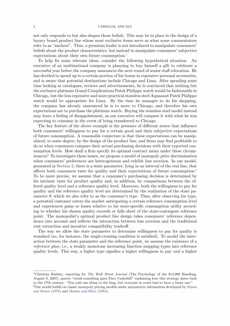
The combined effect of TS∗(q, θ) and LS(q, θ) in the objective function implies thatthere is now, in addition to the kink at r(θ), a discontinuous jump downward (see Figure 3below). The full solution to the firm’s design problem is presented below.

Proposition 4. Given a reference plan θ 7→ r(θ), the optimal incentive feasible contractmenu offered by the firm to loss-averse consumers consists of quality–price schedules θ 7→(qsb(θ), psb(θ)) such that:

qsb(θ) =

q∗(θ; ηλ) : r(θ) ≥ q∗(θ; ηλ),

r(θ) : q∗(θ; ηλ) > r(θ) > q∗(θ; η),

r(θ) : q∗(θ; η) ≥ r(θ), θ ≤ θck ,

q∗(θ; η) : q∗(θ; η) ≥ r(θ), θ > θck ,

(10)

where the θck-consumer lies in the k-th subinterval of consumers with q∗(θ; η) ≥ r(θ), and

psb(θ) = v(qsb(θ), θ) −∫ θ

θL

δ(qsb(θ), θ) dθ, (11)

where the selection in the price schedule is given by

δ(qsb(θ), θ) = (1 + µ(θ))mθ(qsb(θ), θ) + (ηλ− µ(θ)) ddθ

(m(r(θ), θ)

)with µ(θ) = ηλ when qsb(θ) ≤ r(θ) and µ(θ) = η otherwise.

µ = ηµ = ηλ

q* (θ; ηλ)q* (θ; η) r (θ)

(a) qsb(θ) = q∗(θ; ηλ)

q* (θ; η) q* (θ; ηλ)

µ = ηλ µ = η

r (θ)

(b) qsb(θ) = r(θ)

q* (θ; η)

µ = η

µ = ηλ

r (θ)

(c) qsb(θ) = q∗(θ; η)

q* (θ; η)

µ = ηµ = ηλ

r (θ)

(d) qsb(θ) = r(θ)

Figure 3. The profit-maximizing quality is determined by the positionand magnitude of the jump

Here we sketch the proof of Proposition 4, leaving the formal arguments to Section 7.

Step 1. If the θ-consumer has a reference quality above q∗(θ; ηλ), then this last constitutesthe optimal offer from the firm; see Figure 3(A). Indeed, this is the unique maximizer ofTS∗(q, θ), and since q∗(θ; ηλ) ≤ r(θ), the lump-sum cost LS(q∗(θ; ηλ), θ) is zero.

Step 2. If the θ-consumer has a reference level that lies between q∗(θ; η) and q∗(θ; ηλ),then the optimal offered quality is r(θ). This follows because the virtual total surplus

16 CARBAJAL AND ELY

TS∗(q, θ) is strictly decreasing for quality levels above the reference point, as µ(θ) = η,and strictly increasing for quality levels below the reference point, as µ(θ) = ηλ, and hereagain the lump-sum cost is zero; see Figure 3(B).

Step 3. If the θ-consumer reference level lies below q∗(θ; η), the optimal offer by thefirm is either q∗(θ; η) or r(θ). To see why, note that the unique maximizer of TS∗(q, θ)is q∗(θ; η) which is above the reference quality r(θ), so that the lump-sum incentive costis active and amounts to LS(q∗(θ; η), θ). There is therefore a tradeoff between the twocomponents of the objective function: choosing q∗(θ; η) to capture efficiency gains andassociated marginal revenues, or eschewing these and relaxing incentive constraints byoffering r(θ) to ensure that this quality offer is viewed as a loss by higher types, thusavoiding the lump-sum cost. The sign of the difference between profits at r(θ) withgain-loss coefficient ηλ, and profits at q∗(θ; η) with gain-loss coefficient η and an activelump-sum cost, depends on this trade-off.

Step 4. When the reference quality level is below but near q∗(θ; η), efficiency gains aresmall, hence the firm is more likely to offer r(θ). This is illustrated in Figure 3(D). Forlower reference qualities, the tradeoff may go the other way, see Figure 3(C). Suppose thereis an subinterval of types in Θ such that r(θ) = q∗(θ; η) at its left and right endpoints,and r(θ) < q∗(θ; η) everywhere else inside the subinterval. Then, it is possible that themonopolist may try to sell their reference levels to consumers with types at both the lowand high ends of this subinterval, and q∗(θ; η) for θ-consumers in the middle range. Asthis pattern violates monotonicity of the quality schedule, it is not implementable.

Step 5. We observe that the reference plan θ 7→ r(θ) and the quality schedule θ 7→ q∗(θ;µ)cross at most finitely many times, for µ = η, ηλ.18 Thus, for any subinterval of types forwhom reference qualities lie below q∗(θ; η), the optimal quality schedule corresponds to oneof the following three cases: either it assigns q∗(θ; η) to each θ-consumer; or alternativelyit assigns r(θ) for each state parameter θ; or there exists a cutoff type θc among them suchthat the firm offers r(θ) to each θ-consumer below θc, and q∗(θ; η) to each θ-consumerin the subinterval above θc. Which possibility is chosen by the firm depends of courseon the details of the model (i.e., consumption valuation, distribution of types, referenceplan, and the value of the gain-loss and loss aversion coefficients).

4.3. Comparative statics. The specifics of price discrimination under loss aversion ex-hibit novel elements, compared to the loss-neutral case. Relatively high reference plansfor low type consumers can generate allocative efficiency gains under loss aversion, asquality offers get closer to the efficient qualities. In particular, there may be an increasein market coverage. High reference plans for high type consumers, on the other hand,can generate quality distortions above and beyond the efficient levels, so that there is anexcess supply of the product attribute. Moreover, it is possible that for a non-negligiblesubset of buyers, the optimal quality schedule is determined entirely by the reference plan.This implies that optimal contract menu may exhibit a degree of complexity —poolingfor some mid-range consumers, preceded and followed by separating contracts— that re-sponds entirely to consumers expectations or aspirational considerations, as captured bythe reference plan, and not to especial features of the cost function or the distribution oftypes. We spell out some of these properties below.

Corollary 1. The following holds under incomplete information. For loss-neutral con-sumers:

1. Optimal qualities offered by the firm coincide with q∗(·; η), independently of thereference plan.

18We are not stating that r and q∗(·;µ) coincide only finitely many times, as it could be that r(θ) = q∗(θ;µ)for a subinterval of the type space, but only that the difference function fµ = r − q∗(·;µ) changes frompositive to negative a finite number of times.


For loss-averse consumers:

2. Downward distortions. If the reference level r(θ) is weakly below q∗(θ; η), then sois the optimal quality offered by the firm.

3. Efficiency gains. If the reference level r(θ) lies between q∗(θ; η) and the loss-neutralefficient level q(θ; η), then so does the optimal quality offered by the firm.

4. Upward distortions. For loss-averse buyers for whom q(θ; η) ≤ q∗(θ; ηλ), if thereference level r(θ) lies above the loss-neutral classic efficiency level, then so doesthe optimal quality offered by the firm.

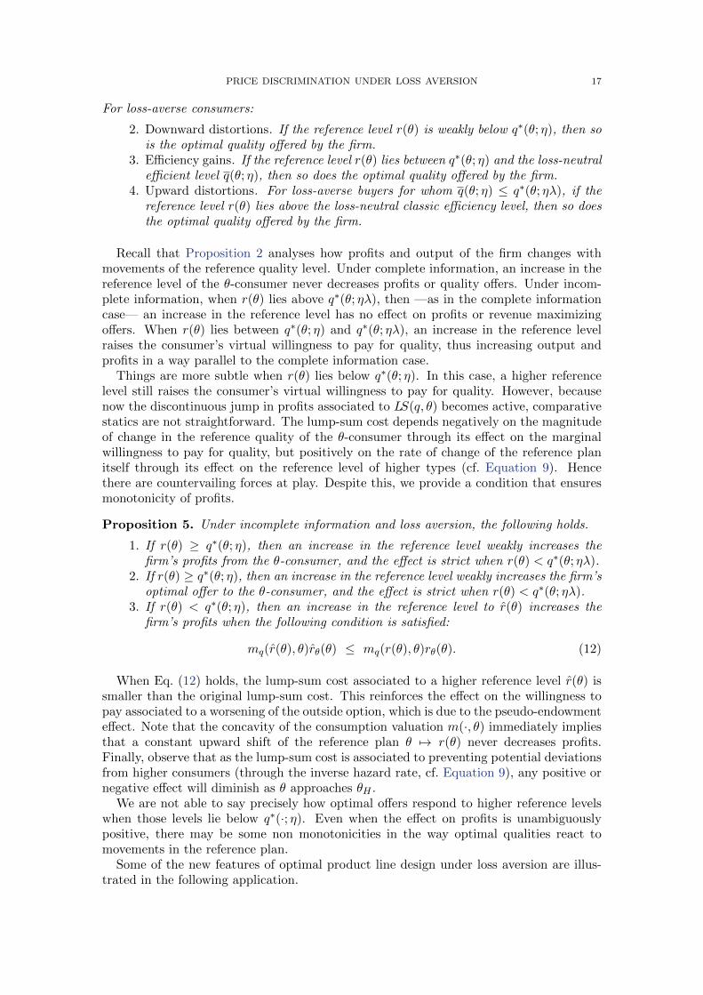
Recall that Proposition 2 analyses how profits and output of the firm changes withmovements of the reference quality level. Under complete information, an increase in thereference level of the θ-consumer never decreases profits or quality offers. Under incom-plete information, when r(θ) lies above q∗(θ; ηλ), then —as in the complete informationcase— an increase in the reference level has no effect on profits or revenue maximizingoffers. When r(θ) lies between q∗(θ; η) and q∗(θ; ηλ), an increase in the reference levelraises the consumer’s virtual willingness to pay for quality, thus increasing output andprofits in a way parallel to the complete information case.

Things are more subtle when r(θ) lies below q∗(θ; η). In this case, a higher referencelevel still raises the consumer’s virtual willingness to pay for quality. However, becausenow the discontinuous jump in profits associated to LS(q, θ) becomes active, comparativestatics are not straightforward. The lump-sum cost depends negatively on the magnitudeof change in the reference quality of the θ-consumer through its effect on the marginalwillingness to pay for quality, but positively on the rate of change of the reference planitself through its effect on the reference level of higher types (cf. Equation 9). Hencethere are countervailing forces at play. Despite this, we provide a condition that ensuresmonotonicity of profits.

Proposition 5. Under incomplete information and loss aversion, the following holds.

1. If r(θ) ≥ q∗(θ; η), then an increase in the reference level weakly increases thefirm’s profits from the θ-consumer, and the effect is strict when r(θ) < q∗(θ; ηλ).

2. If r(θ) ≥ q∗(θ; η), then an increase in the reference level weakly increases the firm’soptimal offer to the θ-consumer, and the effect is strict when r(θ) < q∗(θ; ηλ).

3. If r(θ) < q∗(θ; η), then an increase in the reference level to r(θ) increases thefirm’s profits when the following condition is satisfied:

mq(r(θ), θ)rθ(θ) ≤ mq(r(θ), θ)rθ(θ). (12)

When Eq. (12) holds, the lump-sum cost associated to a higher reference level r(θ) issmaller than the original lump-sum cost. This reinforces the effect on the willingness topay associated to a worsening of the outside option, which is due to the pseudo-endowmenteffect. Note that the concavity of the consumption valuation m(·, θ) immediately impliesthat a constant upward shift of the reference plan θ 7→ r(θ) never decreases profits.Finally, observe that as the lump-sum cost is associated to preventing potential deviationsfrom higher consumers (through the inverse hazard rate, cf. Equation 9), any positive ornegative effect will diminish as θ approaches θH .

We are not able to say precisely how optimal offers respond to higher reference levelswhen those levels lie below q∗(·; η). Even when the effect on profits is unambiguouslypositive, there may be some non monotonicities in the way optimal qualities react tomovements in the reference plan.

Some of the new features of optimal product line design under loss aversion are illus-trated in the following application.

18 CARBAJAL AND ELY

4.4. Price discrimination with uniform signals, linear valuations and quadraticcost. We impose additional assumptions to obtain an explicit solution to the monopolist’sproblem: states are uniformly distributed on Θ = [1, 2]; consumers have a linear consump-tion valuation m(q, θ) = θq; and the firm’s cost function is quadratic, so c(q) = q2/2 + q.Thus, the (pointwise) objective function of the firm is composed of:

TS∗(q, θ) = (1 + µ)(2θ − 2)q − q2/2 − q + (ηλ− µ)(2θ − 2)r(θ), and

LS(q, θ) = (ηλ− µ)(2− θ)θrθ(θ).

Let θµ = (3 + 2µ)/(2 + 2µ), for µ = η, ηλ. Observe θηλ < θη (cf. Figure 4). Readily, oneobtains:

q∗(θ;µ) =

{0 : 1 ≤ θ ≤ θµ,

(1 + µ)(2θ − 2)− 1 : θµ ≤ θ ≤ 2,

as the quality level that maximizes S∗(q, θ;µ).Following the interpretation provided in Section 2.3, we assume that all ex ante identical

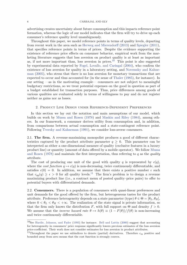
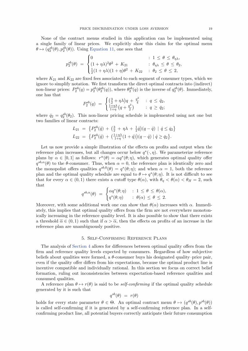
consumers have a common reference plan before state signals are received. To highlightthe effects of the reference consumption plan in terms of optimal design, here we considerthree different plans. Under the first plan θ 7→ r1(θ), consumers naively believe thefirm will offer the (ex ante) expected first best quality level under loss neutrality, sor1(θ) = (1 + η)3/2 − 1 for all θ. Under the second reference plan, consumers anticipatefirst best offers, so r2(θ) = q(θ; η) = (1+η)θ−1 for all θ. Immediately from Proposition 4,the optimal quality schedule qsbi associated with the reference plan ri is given by

qsb1 (θ) =

q∗(θ; ηλ) : 1 ≤ θ ≤ θ1,

r1(θ) : θ1 ≤ θ ≤ θ1,

q∗(θ; η) : θ1 ≤ θ ≤ 2,

and qsb2 (θ) =

{q∗(θ; ηλ) : 1 ≤ θ ≤ θ2,

r2(θ) : θ2 ≤ θ ≤ 2;

where in the first case, θ1 = (7 + 4ηλ + 3η)/(4 + 4ηλ) and θ1 = 7/4, and in the secondcase θ2 = (2 + 2ηλ)/(1 + 2ηλ− η).

Consider a third reference plan θ 7→ r3(θ) defined by r3(θ) = r1(θ)/2 + r2(θ)/2. Aninterpretation is that each θ-consumer puts equal weight into his reference point beingthe loss-neutral efficient quality level, given his type, and the average efficient quality.The optimal offers to consumers with reference qualities below q∗(·; η) depends on thetrade-off between efficiency gains and the lump-sum cost triggered by loss aversion. Forsuch consumers, the difference between profits at r3(θ) and µ = ηλ, and profits at q∗(θ; η)and µ = η (cf. Equation 18 in Section 7) is given by:

4(r3(θ), q∗(θ; η)) = 1

2(1 + η)(ηλ− η)(2− θ)θ − 18(1 + η)2

(3θ − 11

2

)2.

The reference plan r3 and the quality schedule q∗(·; η) intersect at θ = 11/6. Onehas that the difference in profits at θ = 11/6 is strictly positive and the difference inprofits at θH = 2 is strictly negative. Since this profit difference, as a function of types,is continuous and strictly decreasing for all types greater than 11/6, it follows that thereexists a unique cutoff θ3 such that 4(r3(θ3), q

∗(θ3)) = 0. For consumers to the left of θ3,the optimal qualities coincide with reference levels and is below quality schedule q∗(·; η).The optimal quality schedule under r3 is:

qsb3 (θ) =

q∗(θ; ηλ) : 1 ≤ θ ≤ θ3,

r3(θ) : θ1 ≤ θ ≤ θ3,

q∗(θ; η) : θ3 ≤ θ ≤ 2,

where θ3 = (11 + 8ηλ− 3η)/(6 + 8ηλ− 2η).


None of the contract menus studied in this application can be implemented usinga single family of linear prices. We explicitly show this claim for the optimal menuθ 7→ (qsb2 (θ), psb2 (θ)). Using Equation 11, one sees that

psb2 (θ) =

0 : 1 ≤ θ ≤ θηλ,

(1 + ηλ)2θ2 + K21 : θηλ ≤ θ ≤ θ2,12(1 + ηλ)(1 + η)θ2 + K22 : θ2 ≤ θ ≤ 2,

where K21 and K22 are fixed fees associated to each segment of consumer types, which weignore to simplify notation. We first transform the direct optimal contracts into (indirect)non-linear prices: P sb2 (q) = psb2 (θsb2 (q)), where θsb2 (q) is the inverse of qsb2 (θ). Immediately,one has that

P sb2 (q) =

{(32 + ηλ

)q + q2

4 : q ≤ q2,1+ηλ1+η

(q + q2

2

): q ≥ q2;

where q2 = qsb2 (θ2). This non-linear pricing schedule is implemented using not one buttwo families of linear contracts:

L21 ={P sb2 (q) +

(32 + ηλ + 1

2 q)(q − q) | q ≤ q2

}L22 =

{P sb2 (q) +

(1+ηλ1+η (1 + q)

)(q − q) | q ≥ q2

}.

Let us now provide a simple illustration of the effects on profits and output when thereference plan increases, but all changes occur below q∗(·, η). We parameterize referenceplans by α ∈ [0, 1] as follows: rα(θ) = αq∗(θ; η), which generates optimal quality offerqsb,α(θ) to the θ-consumer. Thus, when α = 0, the reference plan is identically zero andthe monopolist offers qualities qsb,0(θ) = q∗(θ; η); and when α = 1, both the referenceplan and the optimal quality schedule are equal to θ 7→ q∗(θ; η). It is not difficult to seethat for every α ∈ (0, 1) there exists a cutoff type θ(α), with θη < θ(α) < θH = 2, suchthat

qsb,α(θ) =

{αq∗(θ; η) : 1 ≤ θ ≤ θ(α),

q∗(θ; η) : θ(α) ≤ θ ≤ 2.

Moreover, with some additional work one can show that θ(α) increases with α. Immedi-ately, this implies that optimal quality offers from the firm are not everywhere monoton-ically increasing in the reference quality level. It is also possible to show that there existsa threshold α ∈ (0, 1) such that if α > α, then the effects on profits of an increase in thereference plan are unambiguously positive.

5. Self-Confirming Reference Plans

The analysis of Section 4 allows for differences between optimal quality offers from thefirm and reference quality levels expected by consumers. Regardless of how subjectivebeliefs about qualities were formed, a θ-consumer buys his designated quality–price pair,even if the quality offer differs from his expectations, because the optimal product line isincentive compatible and individually rational. In this section we focus on correct beliefformation, ruling out inconsistencies between expectation-based reference qualities andconsumed qualities.

A reference plan θ 7→ r(θ) is said to be self-confirming if the optimal quality schedulegenerated by it is such that

qsb(θ) = r(θ)

holds for every state parameter θ ∈ Θ. An optimal contract menu θ 7→ (qsb(θ), psb(θ))is called self-confirming if it is generated by a self-confirming reference plan. In a self-confirming product line, all potential buyers correctly anticipate their future consumption

20 CARBAJAL AND ELY

θηλ θη

r 1

θ1θ1 θHθL

qsb1q( · ; η)

q* ( · ; η)

q* ( · ; ηλ)

θηλ θη θ2θL θH

qsb2

r 2 = q( · ; η)q* ( · ; η)

q* ( · ; ηλ)

θηλ θηθL θHθ3 θ3

r 3

qsb3q( · ; η)

q* ( · ; ηλ)

q* ( · ; η)

Figure 4. The optimal quality schedule qsbi for reference plan ri.

outcomes and take those expectations as their reference quality levels. The set of self-confirming reference plans is clearly non-empty —for example, it contains r = q∗(·, η).While is difficult to provide a full characterization of the set of self-confirming referenceplans, a sufficient condition is readily available (in the following results we maintain theassumptions made in Section 2.2 on reference plans).

Proposition 6. A reference plan θ 7→ r(θ) is self-confirming if one of the followingconditions is satisfied for every θ-consumer:

(a) q∗(θ; ηλ) ≥ r(θ) ≥ q∗(θ; η);(b) q∗(θ; η) > r(θ), and the difference between profits at r(θ) with µ(θ) = ηλ and

profits at q∗(θ; η) with µ(θ) = λ is non-negative.

The above result implies that there exists a multiplicity of self-confirming referenceconsumption plans. On the other hand, the existence of a self-confirming reference plan(partially) below q∗(·; η) depends on the existence of reference plan for which the lump-sum cost associated with loss aversion must be greater than efficiency gains, so that thefirm maintains a non-negligible portion of consumers with r(θ) below q∗(θ; η) at theirreference levels (cf. Equation 18). Note however that any such reference plan will need to


satisfy r(θH) ≥ q∗(θH ; η), as it is impossible for the monopolist to recover informationalrents from higher type buyers by maintaining the θH -consumer at his reference point.

These observations lead to the following question: among all self-confirming optimalcontract menus, which (if any) is the monopolist’s preferred one? The answer, it turnsout, is remarkably simple. Indeed, from Equation 8, the lump-sum cost L(q(θ), θ) isnever incurred when the firm’s offers coincide with consumers’ reference levels, as there isnowhere a change from the loss domain to the gain domain in the consumers’ valuation.Thus, per customer profits in any self-confirming contract menu are

TS∗(r(θ), θ) = S∗(r(θ), θ; ηλ) = (1 + ηλ)m∗(r(θ), θ) − c(r(θ)).

Clearly, this expression is strictly increasing in the reference quality level, for all r(θ) ≤q∗(θ; ηλ). Since we have already established optimal prices for any incentive feasiblequality schedule, it follows that the firm has a unique self-confirming product line, wherethe quality offer for each θ-consumer is q∗(θ; ηλ) and its corresponding price is given byEquation 11.

What about consumers? A higher self-confirming reference consumption plan generatestwo opposite effects on consumer’s welfare. On the one hand, a higher reference levelincreases the informational rents that the monopolist has to give to buyers that are activein the market. On the other, a higher reference level implies a lower value of the outsideoption, due to the pseudo-endowment effect, and this in particular means that activebuyers are worse off (in a self-confirming product line, non-active buyers expect to beexcluded from the market). To analyze these countervailing forces, first notice that,because µ(θ) = ηλ holds at every state in a self-confirming reference plan, the indirectutility for every θ-consumer, after discounting the value of the outside option, is

U(θ)− ηλm(r(θ), θ) =

∫ θ

θL

mθ(r(θ), θ) dθ + ηλ

∫ θ

θL

{mθ(r(θ), θ)−mθ(r(θ), θ)

}dθ (13)

—see Equations (1), (7) and condition (b) of Proposition 3. The first integral in the right-hand side of this expression captures the standard informational rents resulting from thescreening process. It is positive for consumers buying a positive quality offer from thefirm, and because of single crossing (i.e., mqθ > 0), its value increases with a higherreference plan. The second integral captures the value of the informational rents vis-a-vis the participation rents that the consumer concedes to the firm to avoid the outsideoption. Overall, the impact of a higher reference plan depends on the interaction of thesetwo terms, which is also affected by the value of the gain-loss coefficient and the lossaversion coefficient. However, when single crossing has diminishing second order effects,the detrimental effects are relatively small, so that active consumers are also better offwith a higher reference plan.

Proposition 7. The following holds under incomplete information when the firm designsan optimal product line for loss-averse consumers:

1. A higher self-confirming reference plan strictly increases the firm’s profits, when-ever r(θ) ≤ q∗(θ; ηλ).

2. If the function q 7→ mθ(q, θ) is concave for every θ ∈ Θ, then a higher self-confirming reference plan strictly increases consumers’ indirect utility, whenever0 < r(θ) ≤ q∗(θ; ηλ).

3. Under the last hypothesis, the unique preferred self-confirming menu of contractsfor both the firm and consumers is generated by the reference plan θ 7→ r∗(θ) =q∗(θ; ηλ).

Our last result merits some comment, despite its simplicity. First, notice that under itspreferred self-confirming reference plan, the firm exploits consumer loss aversion in twodifferent, albeit related ways. On the one hand, a higher reference plan reduces the value

22 CARBAJAL AND ELY

of the outside option, thus driving up overall net (virtual) consumer surplus. On theother, by offering a quality level equal to the consumer’s reference point, the firm takesadvantage of the higher marginal willingness to pay for each additional unit of quality,which is captured in the choice of the selection used in the Mirrlees representation of theindirect utility to construct the optimal price schedule.

Second, that in our model consumers also prefer r∗ = q∗(·; ηλ) is somewhat counter-intuitive. A higher reference point diminishes the attractiveness of the outside option inthe secondary market, which increases the willingness to pay for quality in the primarymarket served by the firm (recall we are ignoring budgetary restrictions from the part ofthe consumers). Under incomplete information, however, the firm has to pass some of theextra surplus to consumers in the form of information rents, which are increasing in qual-ity. When the effects of the single crossing conditions are diminishing, it follows that thevolume of information rents ceded by the firm to active consumers on the primary marketexceeds the extra participation rents extracted from those consumers when the value ofthe outside option worsens. Thus, active consumers benefit with a higher self-confirmingreference plan.

Third, there are various ways in which the firm may try to induce consumers to adoptits preferred reference plan (this may be the case even if the consumers’ preferred referenceplan were different than the firm’s). For instance, the firm can announce a product lineprior to actual market introduction —we leave aside any cost associated with advertisingcampaigns as they are irrelevant for our argument, as long as marginal advertising costsare small. These announcements can be made in terms of product specification andsalient characteristics, may omit any mention of prices, and will be credible because theycomply with a self-confirming reference consumption plan. This seems consistent withmarketing practices spread across some industries, where both product announcementsand advertising campaigns tend to precede actual market introduction and stress qualityattributes over prices.

Fourth, there are allocative efficiency gains for all θ-consumers for whom q∗(θ; ηλ)lies strictly above q∗(θ; η) —the optimal quality offered to loss-neutral consumers— butbelow q(θ; η) —the efficient quality offered to loss-neutral consumers (see Figure 4). It isthus possible for some buyers with low intrinsic consumption valuation, who under lossneutrality would be excluded from the primary market, to have positive consumptionoutcomes precisely because of higher reference points. For θ-consumers with q∗(θ; ηλ) >q(θ; η) the opposite is true, as these buyers end up with excessive quality levels —i.e.,quality levels above the efficient quality offers to loss-neutral consumers. The expandedrange of the preferred optimal menu of contracts seems to be consistent with stylizedobservations in certain industries (e.g., consumer electronics, luxury goods, etc.) whereproduct lines include goods of increasingly high sophistication.

6. Concluding Remarks

In this paper, we study optimal contract design by a revenue maximizing monopolistwho faces consumers with heterogeneous tastes, reference-dependent preferences and lossaversion. Our paper follows the line of work pioneered by DellaVigna and Malmendier(2004), Eliaz and Spiegler (2006), Koszegi and Rabin (2006), Heidhues and Koszegi (2008),and Orhun (2009) among others, in studying the optimal responses of profit maximizingfirms in a market context with consumers who have systematic behavioral biases.

We find that, while some general insights and intuition of standard price discrimi-nation models are present, the reference consumption plan exerts considerable influencein specifics of the optimal product line. This is due to the appearance of new effectsgenerated by loss aversion under incomplete information. Thus, depending on how po-tential buyers form their expectations of quality consumption, optimal contract menus


may exhibit various distinct features —pooling for intermediate consumers, some discon-tinuities, efficiency gains, upward distortions from efficiency levels, etc.— and thus maynot implemented by simple two-part tariffs.

Our research stresses the importance of understanding how the reference quality lev-els are formed or influenced. Most of the older empirical literature testing reference-dependent price and quality effects consider memory-based models of reference pointformation process (e.g., Hardie, Johnson, and Fader (1993), Briesch, Krishnamurthi,Mazumdar, and Raj (1997), etc.). There is however recent evidence of expectation-based reference points in effort provision both in the field (e.g., Crawford and Meng(2011) and Pope and Schweitzer (2011)) and in the laboratory (e.g., Abeler, Falk, Goette,and Huffman (2011) and Gill and Prowse (2012)). In our monopoly pricing model withstate-contingent reference qualities, there is a multiplicity of expectations-based, consis-tent reference consumption plans, many of which do not rule out marked complexitiesin optimal contracts. On the other hand, the firm’s preferred self-confirming menu ofcontracts exhibits (allocative) efficiency gains and an increased coverage at the low endof the market, and excess supply of quality compared to the efficient quality levels for thehigh end of the market.

That the firm’s preferred self-confirming menu is also the one preferred by consumersrests on higher informational gains being associated to higher quality offers, on the factthat there is no budgetary restrictions and the strict single-crossing condition holds every-where and has diminishing effects (so that informational rents trump participation costsof active consumers). This conclusion may change in a more general model that takes intoaccount other goods and services demanded by consumers as well as initial endowments.Thus, it is important to understand how, in practice, consumers’ (correct) expectationsof future consumption may be influenced by fashion and mode cycles, by social and peerpressure, by directed marketing campaigns, etc. This seems specially important in dy-namic settings where a firm interacts with consumers over multiple time periods via longterm contracts, or where there is short product cycles due to innovation, or in environ-ments of oligopolistic competition where there may be more than one product attributedimension that can be used as a tool to enter the market. We leave these questions forfuture research.

7. Proofs

Proof of Proposition 1.Fix a type θ ∈ Θ and suppose that r(θ) ≥ q(θ; ηλ). The unique maximum of the profitfunction in Equation 2 with µ = ηλ is of course q(θ; ηλ), which generates net revenue tothe firm equal to

TS(q(θ; ηλ), θ) = (1 + ηλ)m(q(θ; ηλ), θ) − c(q(θ; ηλ)). (14)

Choosing q < r(θ) does not change the objective function of the monopolist and strictlyreduces per customer profits TS(q, θ). Choosing an alternative quality level q ≥ r(θ)shifts the objective function in Eq. (2) to incorporate µ = η instead of µ = ηλ. Sincer(θ) > q(θ; η), the monopolist would choose a deviation to q = r(θ) with associated profitsequal to (1 + ηλ)m(r(θ), θ)− c(r(θ)), which are less than or equal to profits derived fromq(θ; ηλ). Hence, the firm has no profitable deviation.

Showing that the revenue maximizing quality level is q(θ; η) when r(θ) ≤ q(θ; η) issimilar and therefore omitted. In this case, profits are equal to

TS(q(θ; η), θ) = (1 + η)m(q(θ; η), θ) + (ηλ− η)m(r(θ), θ) − c(q(θ; η)). (15)

Now suppose that for the θ-consumer, q(θ; η) < r(θ) < q(θ; ηλ). Choosing a qualityq ≥ r(θ) > q(θ; η) leaves us with µ = η in Eq. (2), and thus we are in the strictlydecreasing part of the total surplus. Similarly, choosing q ≤ r(θ) < q(θ; ηλ) yields µ = ηλ

24 CARBAJAL AND ELY

in Eq. (2), so that the monopolist is now in the strictly increasing section of the totalsurplus. It follows that the revenue maximizing quality is r(θ), which generates profitsequal to

TS(r(θ), θ) = (1 + ηλ)m(r(θ), θ) − c(r(θ)). (16)

This completes the proof. �

Proof of Proposition 2.1. Under loss neutrality, the total valuation is v(q, θ) = (1 + η)m(q, θ), independently ofthe consumers’ reference plan. Readily from Equation 2, one has qfb(θ) = q(θ; η) for alltypes θ ∈ Θ.

2. Immediately from Proposition 1.

3–4. Assume that r(θ) < q(θ; η) = qfb(θ). Then optimal revenue for the firm from the θ-consumer is given by Eq. (15). Increasing the reference level to 0 < r(θ) ≤ q(θ; η) does notchange the offered quality but strictly increases profits, as (ηλ−η)mq(r(θ), θ) > 0. When

q(θ; η) < r(θ) = qfb(θ) < q(θ; ηλ), optimal profits for the firm are given by Eq. (16). Thus,an increase in the reference level to r(θ) < r(θ) ≤ q(θ; ηλ) strictly increases the offer fromthe firm to this level and strictly raises profits, since (1 + ηλ)mq(r(θ), θ) − cq(r(θ)) > 0.Finally, when the reference level is q(θ; ηλ) < r(θ), optimal profits are given by Eq. (14).Thus, an increase in the reference level alters neither the optimal offer from the firm nornet revenues. �

Derivation of Equation 5.Fix a quality level q > 0 and assume that the reference plan r is strictly increasing aroundθ, for an arbitrary type θ in the interior of Θ (all remaining cases are similarly obtained).For any θ ∈ Θ, let µ(q, θ) denote the value that µ attains when comparing q to thereference level r(θ). The net total valuation as a function of types is given by:

θ 7→ v(q, θ) = (1 + µ(q, θ))m(q, θ) + (ηλ− µ(q, θ))m(r(θ), θ), (17)

where µ(q, θ) = η if q > r(θ) and µ(q, θ) = ηλ if q ≤ r(θ). The reference plan is apiecewise continuously differentiable function, hence we omit discussion of kinks in thevaluation function due to kinks in the reference plan. This will not have any consequenceon the derivation of optimal contract menu. The function v(q, ·) in (17) has bounded left

and right partial derivatives at θ defined, respectively, by:

v+θ (q, θ) ≡ limθ↓θ

v(q, θ) − v(q, θ)

θ − θand v−θ (q, θ) ≡ lim

θ↑θ

v(q, θ) − v(q, θ)

θ − θ.

Suppose first that r(θ) > q. Then for all types θ sufficiently close to θ, one has µ(q, θ) =

µ(q, θ) = ηλ. It follows that v+θ (q, θ) = v−θ (q, θ) = vθ(q, θ) = (1 + ηλ)mθ(q, θ). Suppose

next that q > r(θ), so that for all types θ sufficiently close to θ, one has µ(q, θ) = µ(q, θ) =

η. It follows that v+θ (q, θ) = v−θ (q, θ) = vθ(q, θ) = (1+η)mθ(q, θ)+(ηλ−η) ddθ(m(r(θ), θ)

).


Finally, suppose that for the θ-consumer, r(θ) = q. Note that for θ′ < θ < θ′′, one has

µ(q, θ′) = η and µ(q, θ) = µ(q, θ′′) = ηλ. By definition, we obtain

v+θ (q, θ) ≡ limθ↓θ

v(q, θ)− v(q, θ)

θ − θ

= limθ↓θ

1

θ − θ

{(1 + µ(q, θ))m(q, θ) + (ηλ− µ(q, θ))m(r(θ), θ)

− (1 + µ(q, θ))m(q, θ) − (ηλ− µ(q, θ))m(r(θ), θ)}

= limθ↓θ

(1 + ηλ)m(q, θ)−m(q, θ)

θ − θ= (1 + ηλ)mθ(q, θ).

Similarly, using the fact that q = r(θ), we have

v−θ (q, θ) ≡ limθ↑θ

v(q, θ)− v(q, θ)

θ − θ

= limθ↑θ

1

θ − θ

{(1 + η)m(q, θ) + (ηλ− η)m(r(θ), θ)

− (1 + ηλ)m(q, θ) ± ηm(q, θ)}

= limθ↑θ

(1 + η)m(q, θ)−m(q, θ)

θ − θ+ lim

θ↑θ(ηλ− η)

m(r(θ), θ)−m(r(θ), θ)

θ − θ= (1 + η)mθ(q, θ) + (ηλ− η) ddθ

(m(r(θ), θ)

).

Note also that v+θ (q, θ) − v−θ (q, θ) = − (ηλ − η)mq(r(θ), θ)rθ(θ) ≤ 0. Thus, for the

θ-consumer, one has that ϕ(q, θ) is equal to the non-empty closed interval[(1 + ηλ)mθ(q, θ) , (1 + η)mθ(q, θ) + (ηλ− η) ddθ

(m(r(θ), θ)

)],

which collapses to a single point when rθ(θ) = 0. �

Proof of Proposition 3.The equivalence between incentive compatibility of contracts θ 7→ (q(θ), p(θ)) and parts(a) and (b) follow from Theorem 1 in Carbajal and Ely (2013). Condition (c) clearlyholds when contracts are individually rational. Suppose now that (c) is also in place.

Using (b) we express U(θ) = U(θL) +∫ θθLδ(q(θ), θ)dθ for any θ-consumer. From (5), any

integrable selection is such that δ(q(θ), θ) ≥ 0, so that U(θ) ≥ 0 follows readily. �

Proof of Proposition 4.Step 1. Suppose that for the θ-consumer one has r(θ) ≥ q∗(θ; ηλ). The unique maximizerof the integrand in the profit function of Equation 8 with µ(θ) = ηλ is precisely q∗(θ; ηλ).Any deviation to an alternative quality q ≤ r(θ) will only hurt profits as it decreasesvirtual total surplus in the objective function without changing the value of the lump-sum cost, which remains at zero. Now consider a deviation to q ≤ r(θ), which switchesµ(θ) in the objective function from ηλ to η. Since r(θ) ≥ q∗(θ; η), it follows by the (strong)concavity of S∗(·, θ; η) that the optimal deviation in this case is q = r(θ). The differencebetween profits at r(θ) and µ(θ) = ηλ, and profits at r(θ) and µ(θ) = η is given by:

(ηλ− η)h(θ)mq(r(θ), θ)rθ(θ) ≥ 0.

It follows that profits at qsb(θ) = q∗(θ; ηλ) and µ(θ) = λ are strictly greater than profitsat r(θ) and µ(θ) = ηλ, which in turn are greater than profits at r(θ) and µ(θ) = η.

26 CARBAJAL AND ELY

Step 2. Suppose that q∗(θ; η) < r(θ) < q∗(θ; ηλ). Consider an alternative quality levelq, such that q > r(θ) > q∗(θ; η). The integrand of Eq. (8) has µ(θ) = η for any such q,so that the lump-sump cost is active. Clearly, profits are strictly decreasing in quality aslong as q > r(θ), so that there is no upward profitable deviation. One can use a similarargument to show that there is no downward profitable deviation from qsb(θ) = r(θ), asany deviation to q < r(θ) has µ(θ) = ηλ. Therefore qsb(θ) = r(θ) is optimal the optimalquality offered by the firm in this case.

Step 3. Suppose that for the θ-consumer, one has r(θ) ≤ q∗(θ; η). As before, the uniquemaximizer of the integrand of the profit function in Eq. (8) with µ(θ) = η is q∗(θ; η). Anydeviation to a quality level q > r(θ) will not change the value of µ(θ) to ηλ and thuswill only decrease profits. Among deviations from q∗(θ; η) to quality levels q ≤ r(θ) thatchange the parameter µ(θ) to ηλ in Eq. (8), thus avoiding the lump-sum cost, the onegenerating the highest profits is q = r(θ). The difference between profits at r(θ) withassociated µ(θ) = ηλ and profits at q∗(θ; η) with associated µ(θ) = η is given by:

4(r(θ), q∗(θ; η)) = (ηλ− η)h(θ)mq(r(θ), θ) rθ(θ)

−{S∗(q∗(θ; η), θ; η)− S∗(r(θ), θ; η)

}. (18)

The sign of the above expression depends on the difference between gains associated withoffering a quality level r(θ), which changes the value of µ(θ) from η to ηλ in the profitfunction for the θ-consumer, cancelling lump-sum transfer to higher type consumers, andefficiency gains in virtual total surplus at µ(θ) = η derived from shifting quality from r(θ)to q∗(θ; η).

Step 4. We formally show the following, from which our statement in the main text willbe derived. Let θ′ < θ′′ be two types for whom q∗(θ′′; η) ≥ q∗(θ′; η) > r(θ′′) > r(θ′) ≥ 0.Then the monopolist either offers to them their respective reference quality levels; orq∗(θ′; η) and q∗(θ′′; η) to each of them, respectively; or it offers to the θ′-consumer hisreference quality level and the quality level q∗(θ′′; η) to the θ′′-consumer.

That one of this possibilities must hold follows from Step 3. Suppose now that for θ′ andθ′′ satisfying the premise of this step, one has instead that qsb(θ′) = q∗(θ′; η) and qsb(θ′′) =r(θ′′). From Proposition 3, it suffices to show a violation of monotonicity: v(r(θ′′), θ′′)−v(r(θ′′), θ′) < v(q∗η(θ

′), θ′′) − v(q∗η(θ′), θ′). It is immediate to see that we can write the

previous inequality as m(r(θ′′), θ′′)−m(r(θ′′), θ′) < m(q∗(θ′; η), θ′′)−m(q∗(θ′; η), θ′). Sinceθ′′ > θ′ and q∗(θ′; η) > r(θ′′), the single-crossing condition on the valuation functionimplies that this inequality is indeed satisfied.

Step 5. From the assumptions in Section 2 it follows that q∗(·;µ) is everywhere continuousand continuously differentiable except possibly at a type where q∗(·;µ) turns from zero topositive. Therefore θ 7→ fµ(θ) = r(θ)− q∗(θ;µ) is continuous and piecewise continuouslydifferentiable, with bounded left and right derivatives everywhere on Θ. Let A ⊂ Θ bethe set of types for which fµ(θ) = 0 and fµθ (θ) 6= 0. Since fµθ (θ) is continuous, it followsthat θ ∈ A is an isolated point and thus A is a discrete subset of a compact set, hence itis finite. The construction of the optimal quality schedule θ 7→ qsb(θ) in Eq. (10) followsfrom the previous steps.

It remains to show that the informational constraints, expressed as conditions (a) to(c) of Proposition 3, are in place. One immediately sees from the expression for incentiveprices in Eq. (11) that both (b) and (c) are in place. To show that condition (a) —integralmonotonicity— is satisfied, let θ′, θ′′ ∈ Θ be two consumer types such that θ′ < θ′′ andsuppose qsb(θ′) < r(θ′) ≤ r(θ′′) < qsb(θ′′) holds —all remaining cases are similarly proven.By construction of the optimal quality offers, there exists a type θc, with θ′ ≤ θc < θ′′,for which one has r(θ′) ≤ r(θc) = qsb(θc) ≤ r(θ′′). Moreover, we can choose θc so thatqsb(θ) ≤ r(θ) for all θ′ ≤ θ ≤ θc, and qsb(θ) > r(θ) for all θc < θ ≤ θ′′.


We first write the valuation differences in a suitable form:

v(qsb(θ′′), θ′′) − v(qsb(θ′′), θ′)

= v(qsb(θ′′), θ′′) − v(qsb(θ′′), θ′) ± v(qsb(θ′′), θc) (19)

≥ v(qsb(θ′′), θ′′) − v(qsb(θ′′), θc) + v(qsb(θc), θc) − v(qsb(θc), θ′).

where the inequality follows from the single crossing property assumed on the consumptionvaluation m(q, θ). A similar argument yields to:

v(qsb(θ′), θ′) − v(qsb(θ′), θ′′) (20)

≥ v(qsb(θ′), θ′) − v(qsb(θ′), θc) + v(qsb(θc), θc) − v(qsb(θc), θ′′).

Notice now that

v(qsb(θ′′), θ′′) − v(qsb(θ′′), θc)

=

∫ θ′′

θc

{(1 + η)mθ(q

sb(θ′′), θ) + (ηλ− η) ddθ(m(r(θ), θ)

)}dθ (21)

≥∫ θ′′

θ∗δ(qsb(θ), θ) dθ,

where the inequality follows from the monotonicity of qsb and the fact that µ(θ) = η for

all θc < θ ≤ θ′′. Furthermore, we can write

v(qsb(θc), θc) − v(qsb(θc), θ′)

≥ (1 + ηλ)m(qsb(θc), θc) − (1 + ηλ)m(qsb(θc), θ′) (22)

=

∫ θc

θ′(1 + ηλ)mθ(q

sb(θc), θ) dθ ≥∫ θc

θ′δ(qsb(θ), θ) dθ,

where as before second inequality follow from the monotonicity of the optimal qualityschedule and the fact that µ(θ) = ηλ for all θ′ ≤ θ ≤ θc. Combining expressions (21) and(22) with Eq. (19), we obtain:

v(qsb(θ′′), θ′′)− v(qsb(θ′′), θ′) ≥∫ θ′′


which is the first inequality of the integral monotonicity condition of Proposition 3.To obtain the second inequality, we write:

v(qsb(θ′), θc) − v(qsb(θ′), θ′) (23)

=

∫ θc

θ′(1 + ηλ)mθ(q

sb(θ′), θ) dθ ≥∫ θc


and similarly

v(qsb(θc), θ′′) − v(qsb(θc), θc)

≤∫ θ′′

θc

{(1 + η)mθ(q

sb(θc), θ) + (ηλ− η) ddθ(m(r(θ), θ)

)}dθ (24)

≤∫ θ′′

θc

δ(qsb(θ), θ) dθ.

Combining expressions (23) and (24) with Eq. (20) above, we obtain the desired inequality.Thus, integral monotonicity is satisfied. �

Proof of Corollary 1.The properties of the optimal offers θ 7→ qsb(θ) follow readily from Equation 10. �

28 CARBAJAL AND ELY

Proof of Proposition 5.1–2. The results are deduced from Proposition 4, and expressions (8) and (9). Indeed,for all r(θ) ≥ q∗(θ; ηλ), the optimal offer is q∗(θ; ηλ) and profits from the θ-consumer areTS∗(q∗(θ; ηλ), θ) = S∗(q∗(θ; ηλ), θ; ηλ), since the lump-sum cost is inactive. For q∗(θ; η) ≤r(θ) < q∗(θ; ηλ), on the other hand, the optimal offer is r(θ) and profits from the θ-consumer are TS∗(r(θ), θ) = S∗(r(θ), θ; ηλ). As r(θ) < q∗(θ; ηλ), this last expression isincreasing in the reference level.

3. Suppose now that r(θ) < q∗(θ; η) for the θ-consumer. Consider a change in the referencelevel to r(θ) such that r(θ) < r(θ) < q∗(θ; η) —the remaining case, when the referencelevel increases above q∗(θ; η), will follow from the analysis below. From Proposition 4,four possibilities emerge.

Case 1. The optimal quality for r(θ) is qsb(θ) = r(θ) and the optimal quality for r(θ)is qsb(θ) = r(θ). Here the lump-sum cost is zero for both optimal offers, thus profitsfrom the θ-consumer are TS∗(r(θ), θ) = S∗(r(θ), θ; ηλ) < S∗(r(θ), θ; ηλ) = TS∗(r(θ), θ),as desired.

Case 2. The optimal quality for r(θ) is qsb(θ) = r(θ) and the optimal quality for r(θ)is qsb(θ) = q∗(θ; η) > r(θ). In this case the lump-sum cost is active at qsb(θ), so thatprofits from the θ-consumer with reference level r(θ) equal TS∗(q∗(θ; η), θ)−LS(q∗(θ; η), θ).However, since r(θ) is an option available to the firm, it must be the case that

TS∗(q∗(θ; η), θ)− LS(q∗(θ; η), θ) ≥ TS(r(θ), θ) = S∗(r(θ), θ; ηλ) > S∗(r(θ), θ; ηλ),

where the last term stands for profits from the θ-consumer when his reference level isr(θ). Thus, per customer profits are strictly greater at r(θ) than at r(θ).

Case 3. The optimal quality for r(θ) is qsb(θ) = q∗(θ; η) and the optimal quality for r(θ)is qsb(θ) = r(θ). In this case, the lump-sum cost is active at qsb(θ) but becomes inactiveat qsb(θ). Consequently, profits from the θ-consumer with r(θ) equal

TS∗(q∗(θ; η), θ)− LS(q∗(θ; η), θ) = S∗(q∗(θ; η), θ; η) + (ηλ− η)m∗(r(θ), θ)

− (ηλ− η)h(θ)mq(r(θ), θ)rθ(θ). (25)

Whereas profits from the θ-consumer with r(θ) equal

TS∗(r(θ), θ) ≥ S∗(q∗(θ; η), θ; η) + (ηλ− η)m∗(r(θ), θ)

− (ηλ− η)h(θ)mq(r(θ), θ)rθ(θ), (26)

where the inequality follows from the fact that q∗(θ; η) was an available alternative forthe monopolist when the reference level is r(θ).

Using Eq. (25) and Eq. (26), we see that the difference in profits for r(θ) and r(θ),which we denote by ∆π(r(θ), r(θ)), is such that

∆π(r(θ), r(θ)) ≥ (ηλ− η)(m∗(r(θ), θ)−m∗(r(θ), θ)

)− (ηλ− η)h(θ)

(mq(r(θ), θ)rθ(θ)−mq(r(θ), θ)rθ(θ)

). (27)

The first term in the right-hand side of the above expression is strictly positive, as thevirtual consumption valuation m∗(·, θ) is strictly increasing in q for q < q∗(θ; η). Thus, asufficient condition for ∆π(r(θ), r(θ)) > 0 is that

mq(r(θ), θ)rθ(θ)−mq(r(θ), θ)rθ(θ) ≤ 0,

which is precisely Eq. (12).

Case 4. The optimal qualities are qsb(θ) = qsb(θ) = q∗(θ; η), so that in both cases thelump-sum cost is active. Here the difference in profits ∆π(r(θ), r(θ)) is equal to theright-hand side of Eq. (27). Thus the previous condition is also sufficient. �


Proof of Proposition 6.When for any θ-consumer one has q∗(θ; ηλ) ≥ r(θ) ≥ q∗(θ; η), it follows immediatelyfrom Eq. (10) that qsb(θ) = r(θ). Now suppose that q∗(θ; η) is strictly greater thanr(θ) for some θ-consumer. Then, from Proposition 4, the optimal quality level is eitherqsb(θ) = q∗(θ; η) or qsb(θ) = r(θ). By (b), one has that the monopolist chooses r(θ) inthis case. Thus the reference plan is self-confirming. �

Proof of Proposition 7.1. Consider expected profits for the firm generated by any self-confirming reference planθ 7→ r(θ). From Eq. (8), when qsb(θ) = r(θ) for all buyers, one has

Πsb =

∫ θH

θS∗(r(θ), θ; ηλ) f(θ) d(θ).

For each state θ ∈ Θ, per customer profits equal S∗(q, θ; ηλ) and are strictly increasingin q, for all q < q∗(θ; ηλ), strictly decreasing in q for all q > q∗(θ; ηλ) and attain a uniquemaximum at q = q∗(θ; ηλ). Thus, per customer profits are strictly increasing in the self-confirming reference level, for r(θ) ≤ q∗(θ; ηλ), with this last being the firm’s preferredreference level.

2. For any given quality level q, from single crossing we obtain that mqθ(q, θ) > 0. Thus,when the self-confirming reference quality plan specifies a positive quality level for theθ-consumer, an increase in the reference level also increases value of the first integral inthe right-hand side of Eq. (13). On the other hand, when the function q 7→ mθ(q, θ) is

concave for all θ ∈ Θ, we obtain that mqqθ(q, θ) is non-negative for all quality levels q.

Since r(θ) ≤ r(θ) holds for all θL ≤ θ ≤ θ, we have that the value of the second integralof Eq. (13) is non-negative as well. The result is now established.

3. This follows immediately from the previous two points of the proposition. �

References

Abeler, J., A. Falk, L. Goette, and D. Huffman (2011): “Reference points andeffort provision,” American Economic Review, 101(2), 470–492.

Ariely, D., and I. Simonson (2003): “Buying, bidding, playing, or competing? Valueassessment and decision dynamics in online auctions,” Journal of Consumer Psychology,13(1-2), 113–123.

Bell, D. R., and J. M. Lattin (2000): “Looking for loss aversion in scanner panel data:the confounding effect of price response heterogeneity,” Marketing Science, 19(2), 185–200.

Briesch, R. A., L. Krishnamurthi, T. Mazumdar, and S. P. Raj (1997): “Acomparative analysis of reference price models,” Journal of Consumer Research, 24(2),202–214.

Carbajal, J. C., and J. C. Ely (2013): “Mechanism design without revenue equiva-lence,” Journal of Economic Theory, 148(1), 104–133.

Crawford, V. P., and J. Meng (2011): “New York City cab drivers’ labor supplyrevisited: reference-dependent preferences with rational-expectations targets for hoursand income,” American Economic Review, 101(5), 1912–1932.

De Giorgi, E. G., and T. Post (2011): “Loss aversion with a state-dependent referencepoint,” Management Science, 57(6), 1094–1110.

DellaVigna, S., and U. Malmendier (2004): “Contract design and self-control: the-ory and evidence,” Quarterly Journal of Economics, 119(2), 353–402.

Eisenhuth, R. (2012): “Reference dependent mechanism design,” Discussion paper,Northwestern University.

30 CARBAJAL AND ELY

Eliaz, K., and R. Spiegler (2006): “Contracting with diversely naive agents,” Reviewof Economic Studies, 73(3), 689–714.

Fogel, S., D. Lovallo, and C. Caringal (2004): “Loss aversion for quality in con-sumer choice,” Australian Journal of Management, 29(1), 45–63.

Galperti, S. (2011): “Commitment, Flexibility, and Optimal Screening of Time Incon-sistency,” Discussion paper, Northwestern University.

Gill, D., and V. Prowse (2012): “A structural analysis of disappointment aversion ina real effort competition,” American Economic Review, 102(1), 469–503.

Grubb, M. D. (2009): “Selling to overconfident consumers,” American Economic Re-view, 99(5), 1770–1807.

Hahn, J.-H., J. Kim, S.-H. Kim, and J. Lee (2012): “Screening loss averse consumers,”Discussion paper, Seoul National University.

Hardie, B. G. S., E. J. Johnson, and P. S. Fader (1993): “Modeling loss aversionand reference dependence effects on brand choice,” Marketing Science, 12(4), 378–394.

Heidhues, P., and B. Koszegi (2008): “Competition and price variation when con-sumers are loss averse,” American Economic Review, 98(4), 1245–1268.

(2012): “Regular prices and sales,” Forthcoming: Theoretical Economics.Herweg, F., and K. Mierendorff (2013): “Uncertain demand, consumer loss aversion,

and flat-rate tariffs,” Journal of the European Economic Association, 11(2), 399–432.Heyman, J. E., Y. Orhun, and D. Ariely (2004): “Auction fever: the effect of oppo-

nents and quasi-endowment on product valuations,” Journal of Interactive Marketing,18(4), 7–21.

Kamenica, E. (2008): “Contextual inference in markets: on the informational contentof product lines,” American Economic Review, 98(5), 2127–2149.

Karle, H. (2013): “Creating attachment through advertising: loss aversion and pre-purchase information,” Discussion paper, ETH Zurich.

Koszegi, B., and M. Rabin (2006): “A model of reference-dependent preferences,”Quarterly Journal of Economics, 121(4), 1133–1165.

Krishna, V., and E. Maenner (2001): “Convex potentials with an application tomechanism design,” Econometrica, 69(4), 1113–1119.

Lambrecht, A., K. Seim, and B. Skiera (2007): “Does uncertainty matter? Con-sumer behavior under three-part tariffs,” Marketing Science, 26(5), 698–710.

Lambrecht, A., and B. Skiera (2006): “Paying too much and being happy aboutit: existence, causes, and consequences of tariff-choice biases,” Journal of MarketingResearch, 43(2), 212–223.

Lange, A., and A. Ratan (2010): “Multi-dimensional reference-dependent preferencesin sealed-bid auctions – how (most) laboratory experiments differ from the field,” Gamesand Economic Behavior, 68(2), 634–645.

Maskin, E., and J. Riley (1984): “Monopoly with incomplete information,” RANDJournal of Economics, 15(2), 174–196.

Milgrom, P. R., and I. Segal (2002): “Envelope theorems for arbitrary choice sets,”Econometrica, 70(2), 583–601.

Mussa, M., and S. Rosen (1978): “Monopoly and product quality,” Journal of Eco-nomic Theory, 18(2), 301–317.

Myerson, R. B. (1981): “Optimal auction design,” Mathematics of Operations Research,6(1), 58–73.

Novemsky, N., and D. Kahneman (2005): “The boundaries of loss aversion,” Journalof Marketing Research, 42(2), 119–128.

Orhun, A. Y. (2009): “Optimal product line design when consumers exhibit choiceset-dependent preferences,” Marketing Science, 28(5), 868–886.


Pope, D. G., and M. E. Schweitzer (2011): “Is Tiger Woods loss averse? Persistentbias in the face of experience, competition, and high stakes,” American EconomicReview, 101(1), 129–157.

Rosato, A. (2013): “Selling substitute goods to loss-averse consumers: limited availabil-ity, bargains, and rip-offs,” Discussion paper, University of California Berkeley.

Simonson, I. (1989): “Choice based on reasons: the case of attraction and compromiseeffects,” Journal of Consumer Research, 16(2), 158–174.

Spiegler, R. (2011): “Monopoly pricing when consumers are antagonized by unexpectedprice increases,” Forthcoming: Economic Theory.

Sugden, R. (2003): “Reference-dependent subjective expected utility,” Journal of Eco-nomic Theory, 111(2), 172–191.

Thaler, R. (1985): “Mental accounting and consumer choice,” Marketing Science, 4(3),199–214.

Tversky, A., and D. Kahneman (1991): “Loss aversion in riskless choice: a reference-dependent model,” Quarterly Journal of Economics, 106(4), 1039–1061.

Williams, S. R. (1999): “A characterization of efficient, Bayesian incentive compatiblemechanisms,” Economic Theory, 14(1), 155–180.

School of Economics, The University of New South WalesE-mail address: [email protected]

Department of Economics, Northwestern UniversityE-mail address: [email protected]

Documents

A MODEL OF PRICE DISCRIMINATION UNDER LOSS AVERSION … · A MODEL OF PRICE DISCRIMINATION UNDER LOSS AVERSION AND STATE-CONTINGENT REFERENCE POINTS ... Gabriele Gratton, Paul Heidhues,