Embed Size (px)
Citation preview
Session Number : 4D
Time: Tuesday, August 26, PM
Paper Prepared for the 30th General Conference ofThe International Association for Research in Income and Wealth
Portoroz, Slovenia, August 24-30, 2008
A Model-Based Multidimensional Capability Deprivation IndexPaola Ballon and Jaya Krishnakumar
For additional information please contact:Paola Ballon or Jaya KrishnakumarDepartment of EconometricsUniversity of GenevaUNI-MAIL, 40Bd. du Pont d’Arve, CH-1211Geneva 4, Switzerland.
Email address:[email protected]@metri.unige.ch
This paper is posted on the following website http://www.iariw.org
1
Abstract
This paper proposes a multidimensional capability deprivation index basedon a structural economic model (SEM) that explains the capability/deprivationlevels in different dimensions, accounting for their multidimensionality andtheir "unobservable" (latent) nature. Under this framework, the freedom ofchoice in each capability domain is represented by a latent variable, partiallyobserved through a group of indicators (achievements), and explained by a col-lection of exogenous variables. The estimators of the different latent variables(scores) provide a measure of the capability levels of the population observed ineach dimension. Single and multi-dimensional capability deprivation indicesare derived using these scores. The proposed indices are ordinal and fulfill aset of desirable properties in the capability framework. The methodology is ap-plied to analyse the deprivation situation of children in Bolivia in the knowledgeand living conditions domains.
Keywords: Capability Approach, Structural Equation Model (SEM), Poverty,Education, Living Conditions, Bolivia.
JEL classification codes: C3, I21, I31, O54.
2
1 Introduction
In recent decades the assessment of poverty 1 has shifted to a multidimensionalperspective to account for the many-sided nature of human deprivation. It is nowwidely accepted that traditional income-based measures are not informative enoughto adequately target the most vulnerable groups, and alternative measures includingnon income-based measures are necessary for improving the design and effective-ness of anti-poverty policies.
This line of thinking has greatly been influenced by the Capability Approach 2.By focusing on the real opportunities that people face (capability sets) this freedom-based approach has opened the ground of a novel line of research on the space ofcapabilities. Though, it is no doubt a more complete framework for poverty assess-ment compared to approaches based only on achievements or resources or both, itsoperationalization and practical applicability has been particularly challenging dueto its informational and methodological requests.
In addition, the appraisal of poverty in a multidimensional setting brings intoconsideration several issues, among which the key issues are the selection of thedimensions and their corresponding indicators, and the aggregation of indicatorswithin and across dimensions . Although both are equally important, the latter re-quires more attention. This leads us to distinguish between the different ’levels’ ofmulti-dimensionality considered in the study of poverty. We would like to stress twoof these that are key to our discussion levels the ’indicator’ level and the ’dimension’level. While informative, the study of the many-dimensions of poverty without dif-ferentiating between the two, might be restrictive. A more suitable level of analysiswould be one based on multiple dimensions and multiple indicators. At all levelsthe choice of the aggregation method (statistical or axiomatic) is important due toits influence on the selection of weights used to obtain the composite index, and therelative importance of the various aspects reflected in the inherent dimensions.
This paper is a contribution along these directions. We propose a multidimen-sional deprivation index based on an operationalization of the capability approach.This measure, understood as a capability deprivation index, differs from earlier lit-erature on multidimensional poverty assessment in the following: (i) it results froman economic model that explains the different dimensions of poverty instead ofsimply describing it, (ii) it measures poverty in the functioning-capability space,(iii) it belongs to a class of multiple dimension(capability domains)-multiple indi-cator(functionings) indices, (iv) it is an ordinal measure fulfilling a set of desirableproperties that represent value judgments and ethical principles in the capabilityframework, (v) it combines statistical and axiomatic methods, at the indicator anddimension levels respectively, for deriving an overall measure of deprivation. We
1Although poverty and deprivation are used interchangeably in this section, in the rest of the paperthe term deprivation is used to denote poverty in the capability space. This is discussed in detail inSection 3.
2Among other approaches towards multi-dimensionality one can cite the Social Exclusion ap-proach (Townsend, 1979; European-Foundation, 1995; Clert, 1999), and the Participatory Approach(Chambers, 1994).
3
apply it empirically to study the deprivation in the capability domains of knowledgeand living conditions for Bolivia’s children in 2002. Our results show that depriva-tion in the single and bi-dimensional cases is more severe in rural areas than in ur-ban and for males compared to females. The bi-dimensional index also shows thatdeprivation increases as the the degree of substitution between both dimensionsdecreases.
We begin the paper by discussing the different approaches to multi-dimensionalityin poverty assessment in Section 2. Section 3 then describes our operationalizationof the Capability Approach through a latent variable model and the estimation ofcapability indices (factor scores). The study of poverty in the capability space ispresented in Section 4. This section first describes the notion of "deprivation" as-sociated with capability poverty and then, proposes two axioms that relate this con-cept to the economic model of section 3. These axioms are doubly important. Theyprovide the theoretical basis for (i) relying on scores as measures of the well-beingand deprivation levels of individuals, (ii) and for defining the individual deprivationfunction required for the assessment of overall-deprivation. This is treated at theend of the section where emphasis is given to the two levels of multidimensionalityaddressed in this paper. The resulting measures are ordinal and consider aggrega-tion within a capability domain (single dimension) and between different capabilitysets (multiple dimensions). Section 5 implements these measures for studying thedeprivation in education and living conditions capabilities of Bolivia’s children in2002. Non-parametric bootstrap samples are used to robustify the results of the val-ues of the scores. Section 6 concludes.
2 Different approaches to multi-dimensionality
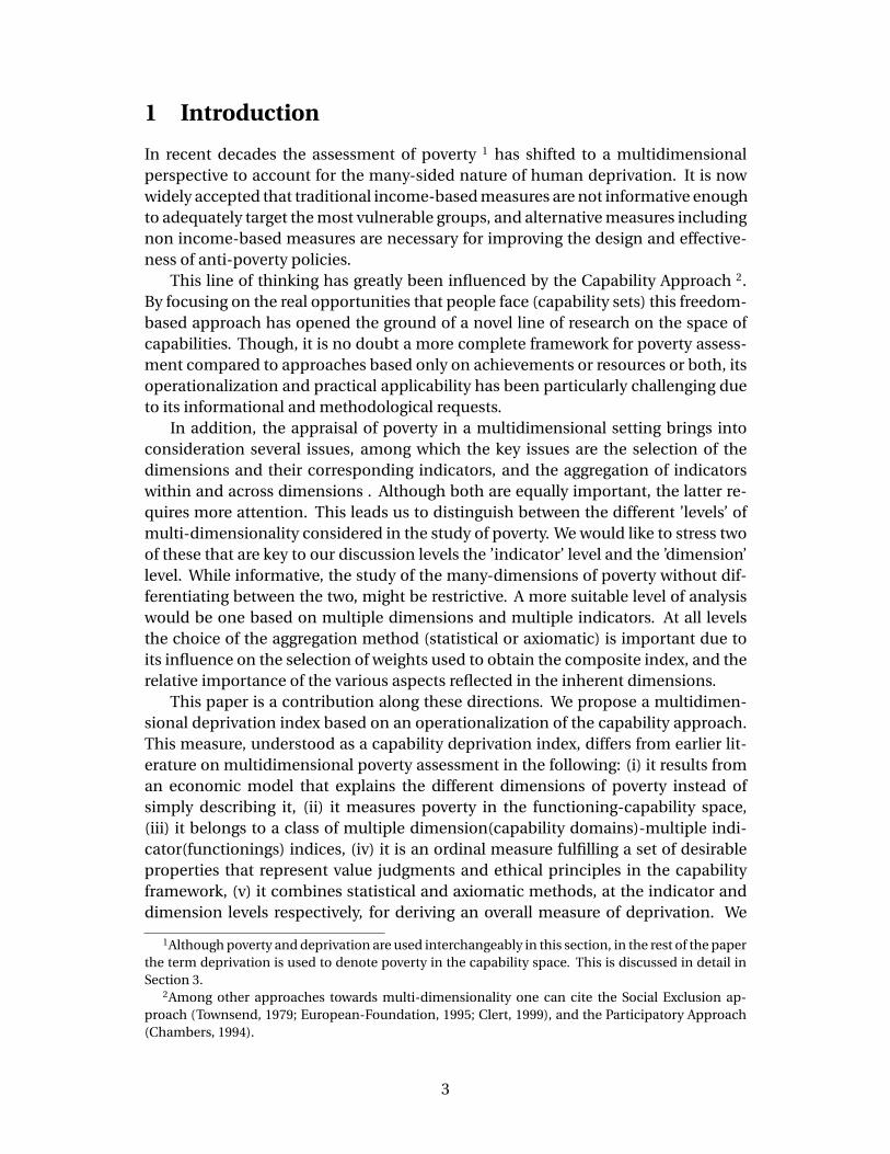
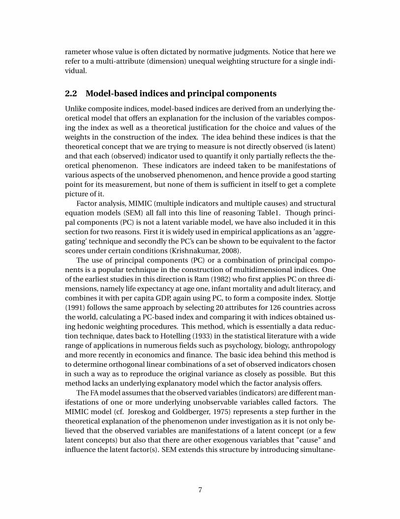
In the study of the many-dimensions of poverty one can distinguish between twolevels of multi-dimensionality: the ’indicator’ level and the ’dimension’ level. Theformer, concerns the number of indicators used to summarize the information ina given dimension. The latter, regards the number of dimensions included in thestudy of poverty. In general their multiplicity leads to four combinations: singledimension-single indicator, single dimension-multiple indicators, multiple dimensions-single indicator, and multiple dimensions-multiple indicators (Figure 1). Single di-mension poverty measures have extensively been used in economic poverty studies,where, the emphasis lies on the income/consumption dimension of poverty, and onthe use of monetary indicators for its evaluation. The employment of multiple in-dicators and multiple dimensions in poverty assessment conforms to the awakenedinterest of practitioners in quantifying the many-sided nature of human deprivationand this is precisely the direction that we have attempted to follow in this paper.
4
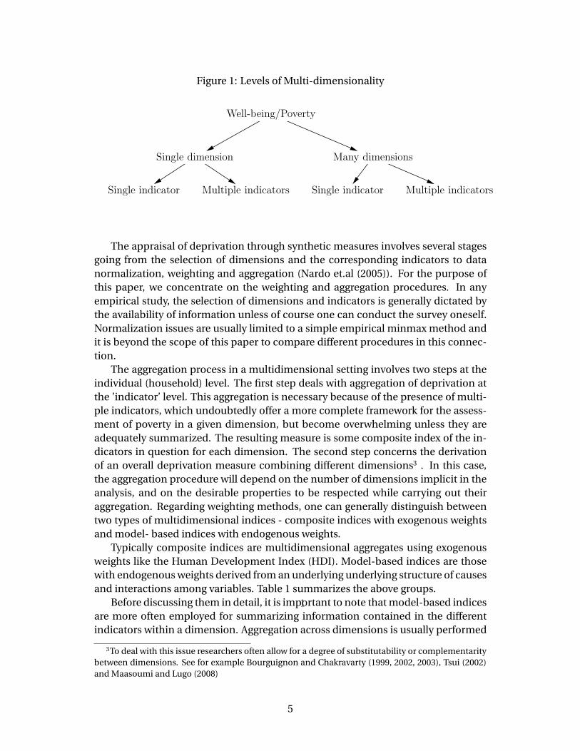
Figure 1: Levels of Multi-dimensionality
Well-being/Poverty
Many dimensionsSingle dimension
Single indicator Multiple indicators Single indicator Multiple indicators
1
The appraisal of deprivation through synthetic measures involves several stagesgoing from the selection of dimensions and the corresponding indicators to datanormalization, weighting and aggregation (Nardo et.al (2005)). For the purpose ofthis paper, we concentrate on the weighting and aggregation procedures. In anyempirical study, the selection of dimensions and indicators is generally dictated bythe availability of information unless of course one can conduct the survey oneself.Normalization issues are usually limited to a simple empirical minmax method andit is beyond the scope of this paper to compare different procedures in this connec-tion.
The aggregation process in a multidimensional setting involves two steps at theindividual (household) level. The first step deals with aggregation of deprivation atthe ’indicator’ level. This aggregation is necessary because of the presence of multi-ple indicators, which undoubtedly offer a more complete framework for the assess-ment of poverty in a given dimension, but become overwhelming unless they areadequately summarized. The resulting measure is some composite index of the in-dicators in question for each dimension. The second step concerns the derivationof an overall deprivation measure combining different dimensions3 . In this case,the aggregation procedure will depend on the number of dimensions implicit in theanalysis, and on the desirable properties to be respected while carrying out theiraggregation. Regarding weighting methods, one can generally distinguish betweentwo types of multidimensional indices - composite indices with exogenous weightsand model- based indices with endogenous weights.
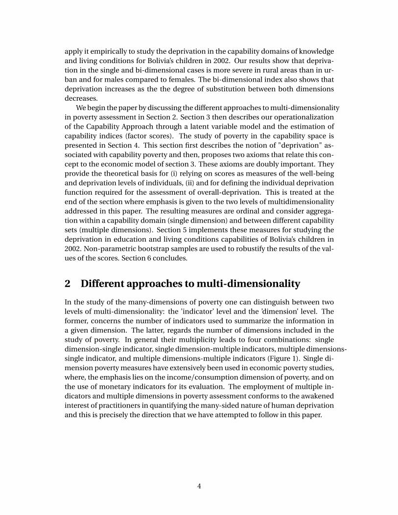
Typically composite indices are multidimensional aggregates using exogenousweights like the Human Development Index (HDI). Model-based indices are thosewith endogenous weights derived from an underlying underlying structure of causesand interactions among variables. Table 1 summarizes the above groups.
Before discussing them in detail, it is important to note that model-based indicesare more often employed for summarizing information contained in the differentindicators within a dimension. Aggregation across dimensions is usually performed
3To deal with this issue researchers often allow for a degree of substitutability or complementaritybetween dimensions. See for example Bourguignon and Chakravarty (1999, 2002, 2003), Tsui (2002)and Maasoumi and Lugo (2008)
5
using axiomatic criteria, although statistical procedures (model-based) may also betheoretically applied. The preference for normative exogenous weights when com-bining different dimensions derives from ethical considerations characterizing thedetermination of the relative importance of different dimensions. From an ethicalpoint of view, the assignment of weights should rely on some normative principlesthat the society would like to follow.
Table 1: Summary of Multidimensional Indices
For model based indicesExogenous Simultaneous
Index Type of weight Causes relationsamong latent
variablesComposite or crude measure Exogenous no noPrincipal Components Endogenous no no
but no underlying modelModel-based
FA Endogenous no noMIMIC Endogenous yes no
SEM Endogenous yes yes
2.1 Composite indices with exogenous weights
Such indices are characterized by the subjective nature of weighting and aggregat-ing structures as it is the analyst or the user who decides on the weights of thedifferent components and the aggregation procedure. In other words, the aggre-gation scheme and the weights are selected exogenously. The criteria used for thechoice of indicators are often based on the relevance and importance of the indi-cator to the concept under study. The Human Development Index (HDI) developedsince 1990 by the United Nations Development Programme is a clear example of thistype of index. It follows a broad definition of human development and gives equalweight (1/3) to three dimensions of human life -longevity, knowledge and decentliving standards; further these dimensions, expressed as normalized (0-1) indices,are aggregated by a simple mean (UNDP, 1990). Other examples could be found inBandura(2006) who surveys 130 indices and Nardo et.al (2005) who examine the dif-ferent stages in the construction of composite indices. It is important to notice thatcomposite indices lack an explanatory model, their theoretical framework relies ex-clusively on the researcher’s assessment of the real-world phenomenon.
In addition to equal weighting schemes which produce simple averages, we alsofind in the literature unequal exogenous weighting structures such as the multidi-mensional human poverty index (Anand and Sen, 1997) where the weights are un-equal but still decided unilaterally by the analyst. Typically they involve some pa-
6
rameter whose value is often dictated by normative judgments. Notice that here werefer to a multi-attribute (dimension) unequal weighting structure for a single indi-vidual.
2.2 Model-based indices and principal components
Unlike composite indices, model-based indices are derived from an underlying the-oretical model that offers an explanation for the inclusion of the variables compos-ing the index as well as a theoretical justification for the choice and values of theweights in the construction of the index. The idea behind these indices is that thetheoretical concept that we are trying to measure is not directly observed (is latent)and that each (observed) indicator used to quantify it only partially reflects the the-oretical phenomenon. These indicators are indeed taken to be manifestations ofvarious aspects of the unobserved phenomenon, and hence provide a good startingpoint for its measurement, but none of them is sufficient in itself to get a completepicture of it.
Factor analysis, MIMIC (multiple indicators and multiple causes) and structuralequation models (SEM) all fall into this line of reasoning Table1. Though princi-pal components (PC) is not a latent variable model, we have also included it in thissection for two reasons. First it is widely used in empirical applications as an ’aggre-gating’ technique and secondly the PC’s can be shown to be equivalent to the factorscores under certain conditions (Krishnakumar, 2008).
The use of principal components (PC) or a combination of principal compo-nents is a popular technique in the construction of multidimensional indices. Oneof the earliest studies in this direction is Ram (1982) who first applies PC on three di-mensions, namely life expectancy at age one, infant mortality and adult literacy, andcombines it with per capita GDP, again using PC, to form a composite index. Slottje(1991) follows the same approach by selecting 20 attributes for 126 countries acrossthe world, calculating a PC-based index and comparing it with indices obtained us-ing hedonic weighting procedures. This method, which is essentially a data reduc-tion technique, dates back to Hotelling (1933) in the statistical literature with a widerange of applications in numerous fields such as psychology, biology, anthropologyand more recently in economics and finance. The basic idea behind this method isto determine orthogonal linear combinations of a set of observed indicators chosenin such a way as to reproduce the original variance as closely as possible. But thismethod lacks an underlying explanatory model which the factor analysis offers.
The FA model assumes that the observed variables (indicators) are different man-ifestations of one or more underlying unobservable variables called factors. TheMIMIC model (cf. Joreskog and Goldberger, 1975) represents a step further in thetheoretical explanation of the phenomenon under investigation as it is not only be-lieved that the observed variables are manifestations of a latent concept (or a fewlatent concepts) but also that there are other exogenous variables that "cause" andinfluence the latent factor(s). SEM extends this structure by introducing simultane-
7
ity among the latent variables in the structural explanation4 . This structure is highlyrelevant in our context as it provides us with a framework for operationalizing the ca-pability approach, acknowledging its indirect measurement, and assessing povertyin the capability space. It also offers an explanatory framework of the causes of ca-pability poverty and interactions among its dimensions, which is fundamental forunderstanding the phenomenon and for making policy decisions.
The use of non-statistical methods comprises scaling techniques and fuzzy setstheory. The scaling of functionings consists in a projection of each variable onto a 01range, which are further aggregated into a composite measure. The Human Devel-opment Index and the Human Poverty Index (UNDP, 1997-2008) are the two majorexamples of the employment of such techniques, and are widely accepted as the firstmajor operationalizations of the CA in the space of observed functionings. Follow-ing the classification provided in Table1, we could classify them as two-level indicesbelonging to the class of multiple dimensions-multiple indicators, with exogenousweights (at both levels). The dimensions, in this case, correspond to observed func-tionings and the indicators their corresponding measures. Fuzzy sets methodologyis a mathematical tool used to provide a summary measure of the "degree" of povertyor well-being associated to the distribution of functionings under analysis. In thiscase, poverty is not a zero or one concept but rather "a broad and opaque" one (Sen,1992). Cerioli and Zani (1990) and Cheli and Lemmi (1995) have applied it to thestudy of well-being measurement in general, while Chiappero-Martinetti (2000) andLelli (2000) to functionings in particular.
3 Operationalization of the Capability Approach throughLatent Variable Modelling
In this section we describe the main features characterizing the Capability approachand its operationalization through a structural equation model (SEM). Our mainconcern is the estimation of the latent variables or capability indices, in our case,which provide a measure of the well-being status of individuals in the different ca-pability domains. These are presented at the end of the section.
According to Sen (1985), (1992), (1993), (1999), the basic purpose of developmentis to enlarge people’s choices so that they can lead the life they want to. This notion offreedom is the essence of the Capability Approach (CA). Under this framework, thechoices that one has are termed "capabilities" and the levels of achievement in thesecapability domains are called "functionings". Resources or entitlements (commodi-ties and their characteristics) lack of an intrinsic value and are rather instrumen-tal. In other words, functionings are the individual’s "beings" and "doings" resultingfrom a given choice, capabilities are all the possible functionings that the individ-ual can achieve, and resources are the means to achieve. The conjunction of thesethree notions (capabilities, functionings and resources) leads to a conversion pro-cess of resources to possible functionings which is individual-specific, influenced
4See e.g. Bollen (1989), Muthen (2002), and Skrondal and Rabe-Hesketh (2004) for a survey.
8
by personal, social and cultural characteristics. Thus, in this approach, human de-velopment is understood as the enhancement of the set of choices or capabilitiesof individuals, and poverty corresponds to a notion of deprivation defined as theindividual’s inability to achieve "minimal" functionings.
Operationalization of the CA, assessing either well-being or the lack of it, hasbeen particularly challenging due to its informational and methodological require-ments. Further, there is no common agreement about which dimensions ought tobe included, nor how they should be summarized. To make it operational, com-posite indices have been constructed on the means of statistical and non-statisticalmethods. Yet, the operationalization has mainly concerned the aggregation of func-tionings and/or resources .
The employment of statistical methods in the area of human development andwell-being measurement have essentially been confined to the use of principal com-ponents (Ram, 1982; Slottje, 1991; Klasen, 2000; Rahman, Mittelhammer and Wand-schneider, 2005; Noorbaksh, 2003; McGillivray, 2005), and exploratory factor analy-sis (Schokkaert and Van ootehgem, 2000; Balestrino and Sciclone, 2000; Lelli, 2000;and Maasoumi and Nickelsburg, 1988). SEM have been used by very few authors(Kuklys, 2005; Krishnakumar and Ballon, 2008) and have not been applied so far, toour knowledge, in the field of capability deprivation measurement.
In this paper, we will concentrate on Structural Equation Models as they providea complete framework to take into account the interactions among the different ca-pability dimensions, and the influence of the surrounding environment 5. In a SEMframework, the (not directly observable) degree of freedom in the different dimen-sions relevant for wellbeing and poverty assessment are represented by latent vari-ables, partially observed through a set of indicators, and explained by a collection ofexogenous variables. The estimators of the latent variables provide a measure of theindividual’s capability status in the different dimensions. On the basis of these la-tent variable scores we derive, in section 4, multidimensional capability deprivationindices.The SEM is formalized as follows 6:
ηi =α+Bηi +Γxi +ζi (1)
where ηi is a (m × 1) vector representing the unobserved capability of individual iin each of the m domains; xi is a (k × 1) vector of k exogenous factors representingthe social, cultural and political environment; ζi is a (m ×1) vector representing theunknown omitted factors in the explanation of η that are not explicitly modelled inthe equation (random errors); α, B,Γ are the corresponding coefficient vector andmatrices.
The observed indicators in the different capability domains can either be contin-uous or qualitative variables. In order to be able to treat these two types in a uniform
5See Krishnakumar (2007) for further explanations regarding the adequacy of SEM in the opera-tionalization of the CA.
6For a detailed formalization see Krishnakumar (2007) and Krishnakumar and Ballon (2008).
9
way we introduce a response variable y * i which will be taken to be directly observedin the case of a continuous indicator, and which will be latent and linked to the ob-served variable through a qualitative response model in the case of qualitative data.This gives the following measurement equations:
y∗i = ν +Ληi +D xi +εi , (2)
where y∗i is a (p ×1) vector representing the response variables of individual i ; xi is a(s × 1) vector of s individual characteristics and preferences that have an impact onthe choice process transforming capabilities into functionings; εi is a (p × 1) vectorof random errors; ν,Λ, D are the corresponding coefficient vector and matrices. Inthe case of a continuous observed indicator for individual i in dimension j denotedas yi j , we have:
yi j = y ∗i j , (3)
when the observed indicator is of a qualitative nature, we write:
yi j =
¨1 if y ∗i j >τj
0 otherwise(4)
for a dichotomous indicator, and
yi j = c , if τj ,c < y ∗i j ≤τj ,c+1 (5)
for a categorical indicator.
It is further assumed that:
E (ζi ) = 0, E (εi ) = 0, (6)
V (ζi ) = E (ζi ζ′i ) =Ψ, (7)
V (εi ) = E (εi ε′i ) =Θ. (8)
Thus, the observations are centered without loss of generality, and the distur-bances across individuals are assumed to be homoscedastic and nonautocorrelated.These assumptions do not mean that the individual disturbances from two differentequations need to be uncorrelated nor that they have the same variance. Equations(7) and (8) show that these are full matrices allowing for correlations between differ-ent capability domains and for heteroscedastic variances.
On the basis of these stochastic assumptions, the above nonlinear model is es-timated by minimizing the distance between the sample moments of the observedvariables and the corresponding theoretical moments expressed as a function of theunknown parameters, by generalised method of moments (GMM)(see e.g. Browne,
10
1984). An alternative estimation method is (conditional) maximum likelihood (cf.e.g. Joreskog, 1973; Browne and Arminger, 1995; Muthen, 1984). In this case theparameters are estimated under (conditional) normality of the indicator vector y *given the exogenous variables x and its variance is corrected using the well-known’sandwich’ formula under non-normality (quasi-maximum likelihood, cf. White,1982; Gouriéroux, Monfort and Trognon, 1984).
Factor scores
Once the parameter estimates are obtained, the final step consists in the estimationof the vector of latent variables for each individual i (factor scores), which is of pri-mary interest to us, because these estimators quantify the degree of freedom in eachcapability domain. Factor scores could be estimated by the Empirical Bayes esti-mator or by maximizing the logarithm of their posterior distribution. Both methodslead to similar results. Following the empirical Bayesian approach, which is a stan-dard procedure suggested in the related literature (cf. Skrondal and Rabe-Hesketh,2004), the latent factors are estimated by their posterior means given the sample, re-placing the parameter values by their estimates. In the case of a linear SEM model,with only continuous indicators, the empirical Bayes estimate of the factor scoresis7:
η̂i =n�
I− ΣΛ′ �ΛΣΛ
′+Θ
�−1Λ�
A−1α− �ΣΛ′ �ΛΣΛ
′+Θ
�−1ν�o
+nΣΛ
′ �ΛΣΛ
′+Θ
�−1 y∗i
o
+n�
I − ΣΛ′ �ΛΣΛ
′+ Θ
�−1Λ�
A−1Γxi −�ΣΛ
′ �ΛΣΛ
′+ Θ
�−1D xi�o
(9)
where A = I−B, and Σ = (I−B)−1 Ψ (I−B)′−1. Equation (9) shows that the factorscore results from a combination of three terms: a ’net constant’ term, summarizingthe intercept effect α and ν, an ’indicator’ term reflecting the information containedin y∗i , and a ’net causal’ term resuming the causal effect of the exogenous variablesxi of the measurement and structural equations. It is interesting to note that if wewrite it as,
η̂i =K+W y∗i + W̃p xi (10)
where K, W, and W̃ are matrices of appropriate dimensions, we see that pre-multiplyingmatrices of each term in equation (9) are the associated weights W and W̃ of the vec-tor of indicators y∗i , and of the vector of (net) exogenous causes xi , respectively, andK a constant.The above formula shows that, the capability set for a single individual
7See Krishnakumar and Nagar (2008) for details regarding the derivation.
11
is represented by a composite measure that summarizes the information providedby her achievement indicators and her personal, social and cultural environmentfeatures, in an endogenous manner.
When the observed indicators are both continuous and qualitative the derivationof factor scores becomes more complex and is carried out by iterative techniques(Muthen, 1998-2004). However, it is interesting to note that only first and second or-der (conditional) moments are necessary for obtaining factor scores. This is shownby equation (11), which is equivalent to equation (9) except that it is written in mo-ment terms, the expression is then:
η̂i =µi + ΣΛ′Σ∗−1�y∗i − µ∗i ) (11)
where
µi = E (ηi |xi ) = (I−B)−1 α+(I−B)−1 Γxi , (12)
Σ=V (ηi |xi ) = (I−B)−1Ψ (I−B)′−1 , (13)
are the mean vector and covariance matrix of the (multivariate normal) prior distri-bution of ηi conditional on xi , and
µ∗i = E (y∗i |xi ) = ν + Λµi + D xi , (14)
Σ∗ =V (y∗i |xi ) =ΛΣΛ′+ Θ , (15)
are the conditional expectation and conditional variance of the (latent) responsevariable y∗i , that links a qualitative indicator through a latent response model. Thusfrom (11), we see that to estimate the latent variable vector (capability indices) oneonly needs information on conditional means µi , µ∗i , and conditional variances Σ,Σ∗.
4 Deprivation in the capability space
Formalization
This section formalizes the assessment of deprivation in the capability space usingthe capability/freedom measures derived in the previous section. After some no-tational definitions, we present two axioms that characterize the evaluative space ofcapabilities as measured by factor scores in our model. On this basis we propose twotypes of capability deprivation indices (CDI). One that performs aggregation within a
12
capability domain (single dimension-multiple indicators), and a second that, in ad-dition, combines capability sets across dimensions (multiple dimensions-multipleindicators). Both types of indices are ordinal and satisfy a series of axioms repre-senting ethical principals and value judgements.
Consider a population of i = 1, 2, . . . , n individuals whose degree of freedom (abil-ity to choose) in any capability domain j = 1, 2, . . . ,m is represented by a continuousvariable ηi j (say the true factor score). We will state the definitions and axioms fortrue measures of capabilities ηi j which have to be replaced in practice by their esti-mates η̂i j from the previous section.
Let ηj = (η1j ,η2j , . . . ,ηn j ) denote the j -th capability vector drawn from the j -thcapability space E j =
⋃∞n=1E n
j , where ηi j ∈ E j is some nondegenerate real intervaland E n
j is the set of all n-tuples of elements in E j . Further, assume that the individ-ual capabilities are arranged in an ascending order such that η1j ≤ η2j ≤ · · · ≤ ηn j .Next, let R(.) denote the rank function that maps theηj vector into the set of positiveintegers. This is, R(.) : ηj 7→ Z+ = (1, 2, . . . , n ). For a given individual i ∈ n , his or-dinal position in the distribution of capability scores is given by R(ηi j ) = ri j , whereri j = p , p ∈ Z+ = (1,2, . . . ,n ). Let rj = (r1j , r2j , . . . , rn j ) be the resulting vector of in-creasingly arranged individual ranks in the j -th dimension, with max(rj ) ≤ n andmin(rj ) = 1. For our purposes we set R(η1j ) = r1j = 1. This means that we assign arank of one to the worst off individual i.e., the one exhibiting the lowest score. Lastly,for i 6= i ′ both ∈ n , ri j= ri
′j whenever ηi j=ηi
′j , or in other words, two different indi-
viduals exhibiting the same factor score are ranked equally. Note that the formaliza-tion is written down in terms of the true factor scores η but in practice these will bereplaced by their estimates obtained as explained in the previous section.
We characterize the capability space by the following two axioms:
Axiom 1 (Monotonic freedom of choice) For a given capability domain j and forany two individuals i and i ′ ∈Z+, i is better off than i ′⇔ηi j >ηi
′j .
Axiom 2 (Ordinal freedom of choice) For a given capability domain j and for anytwo individuals i and i ′ ∈Z+,
i is better off than i′⇔ ri j > ri
′j
i is as well as than i′⇔ ri j = ri
′j
where ri j and ri′j denote the ordinal positions of i and i ′ in the distribution of capa-
bility scores, respectively.
Thus the degree of freedom of an individual is represented by her factor score,and her relative position in the whole population by her rank in the ordering ofthe (capability) scores. Individual deprivation and interpersonal comparisons cantherefore be based on a mixture of cardinal and ordinal information regarding thescores, with greater (score) values and higher ranks denoting greater well-being.
13
On the basis of Axioms 1 and 2, and using an absolute notion of capability depri-vation (Sen, 1983), we propose the following definition for identifying the deprivedindividuals in a single capability domain.Let ηd j and rd j denote the factor score and ordinal position of a ’fictitious’ deprivedindividual who only has the capability to achieve a minimal set of functionings. Letus denote this ’minimal’ capability as ηd j ∈ E j .Weak definition of the deprived : For a given deprivation threshold ηd j ∈ E j and forall ηj ∈ E j , the j -th capability deprived domain is S j (ηj ) = {i ∈ E j | ηi j < ηd j ⇒ri j < rd j }, and the number of deprived individuals is qj (ηj ) = c a r d {S j }.The preceding definition takes the deprivation threshold to be the score (and rank)of a "fictitious" individual, denoted by the subscript(d). The term fictitious is usedto recall that it is the analyst who decides what the minimal level of functioningsthat an individual should be able to achieve. According to this definition the set ofdeprived individuals comprises all individuals whose factor score (and thus rank)is smaller than the factor score (and rank) of the fictitious deprived individual. Itis worth noting that using a weak definition of the deprived avoids including thefictitious deprived individual in the deprivation set, which by ’construction’ is thedeprivation threshold.
Deprivation within a capability set
The above definition of the poor and axioms (1) and (2) allow us to characterize in-dividual deprivation, in a given capability domain, as an individual function:
d i j =
(f (ηi j , ri j ;ηd j , rd j ) if i ∈S j
0 otherwise(16)
where f is a continuous function decreasing with respect to ηi j and ri j , and increas-ing with respect to ηd j and rd j . Note that f is not differentiable. Thus, from (16) wesee that the individual deprivation function d i j depends on cardinal (score) and or-dinal (rank) information regarding the individual and the fictitious deprived status.The total deprivation within a capability domain for the whole population can bedefined as follows:
For a given capability domain j and a deprivation threshold ηd j a measure ofaggregate capability deprivation, say a capability deprivation index, is a real-valuedfunction:
D j =G�ηj , rj , j = 1, ..., n ;ηd j , rd j
�=G
�d 1j , d 2j , . . . , d n j
�: E j × Z+ → R+ (17)
where the function G has similar properties as f with respect to its arguments. Clearlythere are an infinite number of f and G functions that satisfy the above conditions.In what follows, we propose some additional properties that the individual depri-vation function f (·) and aggregate function G (·) should satisfy. These propertiesrepresent value judgements and ethical principles in the capability space leading
14
to restrictions on possible functional forms. Under these principles, the resultingmeasure D j would be a distribution-sensitive measure allowing for interpersonalcomparisons. We shall call it a simple capability deprivation index. The term sim-ple is used to mean the analysis of deprivation in a single capability domain withmultiple functioning indicators.
Desirable properties in the capability framework
Inspiring from the literature on economic poverty measurement we propose the fol-lowing desirable properties for our CDI. These could be regarded as "basic" valuejudgements that one would like to incorporate in any quantitative measure to beused as a capability deprivation index.
Definitions
Change in non deprived scores : We say that η̃j ∈ E j is obtained from ηj ∈ E j by achange in non deprived scores if η̃i j = ηi j∀i ∈ S j , and η̃i j 6= ηi j for some i /∈ S j . ByAxiom 2, this will lead to a change in the corresponding rank vector8, where r̃i j willbe different for all i /∈ S j whose ranks were above the rank of the individual whosescore has changed in the initial distribution.
Gain (loss) of freedom of choice9 : We say that η̃j ∈ E j is obtained from ηj ∈ E j
by a gain (loss) of freedom of choice if η̃i j > ηi j (η̃i j < ηi j for some i ∈ S j , andη̃i j =ηi j for every other i ∈S j . By Axiom 2, it will translate into a better (worse) ordi-nal position for the individual whose score has changed10 and the ranks will changefor all individuals whose ranks were above the rank of the individual whose score haschanged in the initial distribution.
Regressive (progressive) transfer : We say that η̃j ∈ E j is obtained from ηj ∈ E j by aregressive (progressive) transfer if there exists a pair of individuals i and i ′, such that:(1) ηi j < ηi
′j , (2) η̃i
′j − ηi
′j > 0; ηi j − η̃i j > 0, (3) ηk j = η̃k j ∀k 6= i , i ′. Equiva-
lently, by Axiom 2 we could express these three conditions in terms of their ordinalrepresentations, say (1) ri j < ri
′j (2) r̃i
′j − ri
′j > 0; ri j − r̃i j > 0
The first condition says that i is more deprived than i ′. The second condition saysthat there is an increase in the freedom of choice of the less deprived individual (i ′)and a decrease in the freedom of choice of the more deprived one (i ). The third con-dition says that the freedom of choice of the remaining individuals does not change.Regarding the ranks, it is clear that the rank of i ′ will increase and that of i will de-crease but it is also easy to understand all the other ranks of individuals who were
8When estimates are used, the change should be “statistically significant" for the ranks to be dif-ferent.
9This definition is equivalent to the simple increment (decrement) definition used by Zheng(1997).
10Once again the gain(loss) of freedom should be “statistically significant" in case of estimates.
15
above the initial rank of i will be different in the new distribution.Now the properties:
Single-dimension Focus axiom. If η̃j ∈ E j is obtained from ηj ∈ E j by a change innon deprived scores then D j = D̃ j . This means that the the deprivation measure de-pends only on the scores of the deprived individuals.
Single-dimension Monotonicity axiom. If η̃j ∈ E j is obtained from ηj ∈ E j by a gain(loss) of freedom of choice, then D j ≤ D̃ j (D j ≥ D̃ j ). This means that for a given de-privation threshold, the degree of deprivation resulting from an improvement (wors-ening) of an individual’s score cannot be greater (smaller).
Single-dimension Transfer axiom. If η̃j ∈ E j is obtained fromηj ∈ E j by a regressivetransfer among the deprived, then D j ≥ D̃ j . This means that whenever the scores oftwo deprived individuals change, with the more deprived one ending with even lessability to choose, the degree of deprivation should not decrease.
Relying on these properties, and recalling the lack of cardinal interpretation ofthe scores, we propose the following characterizations of the individual deprivationfunction in terms of the number of positions that an individual is away from thethreshold position (rank gap):
d i j =�
rd j − ri j�
(18)
The overall capability deprivation index (for a single dimension) can then be de-fined as:
D j =1
n
∑
i∈S j
�d i j� ·ωi j
=1
n
∑
i∈S j
�rd j − ri j
� ·ωi j (19)
with ωi j =ηd j
ηi ji.e. the rank gap is multiplied a ‘weight’ given by the inverse of the
relative distance of the individual score to the deprivation threshold. In other words,the farther away the score of the individual from the threshold in relative terms (i.e.the smaller the relative score), the bigger the weight, thus giving greater importanceto the more deprived.
Alternatively one could also define
d i j =�
rd j − ri j� ·ωi j (20)
incorporating the ‘weight’ directly into the individual deprivation measure and have
16
D j =1
n
∑
i∈S j
�d i j�
(21)
which will yield the same aggregate index.It is easily seen that both ((18)) and ((20)) imply that d i j is decreasing with respect
to ri j and increasing with respect to rd j meaning greater deprivation whenever therank gap increases. If we include the weights, then in addition f becomes decreasingwith respect to ηi j and increasing with respect to ηd j thus satisfying the conditionslaid out earlier.
Regarding the aggregate deprivation within a capability domain, the functionalform of D j in (21) shows that the capability deprivation index is a sort of an aver-age of the individual deprivation functions. We say "sort of" because the individualweights used in its computation do not add up to 1, as is required for weighted av-erages. This however is not necessarily a drawback of the index and is true for otherindices like the classical FGT class poverty indices. Our index gives the average num-ber of ’weighted’ positions that an individual is away from the deprivation threshold.This per capita interpretation seems quite reasonable as it allows to compare differ-ent groups without any additional assumptions on the scale of measurement of thescores. Indeed, any attempt of summarizing the information using the values of thescores as such, and not using them as weights as in our case, needs at least an in-terval scale of measurement for the scores, under which only means and differencesare allowed. If one is interested in performing other operations with scores, then aratio scale is needed (Stevens, 1946). For the moment, we do not assume that ourscores satisfy the above scales of measurement and only consider them as ordinal(continuous) measures.
The above CDI satisfies the properties enumerated in the beginning of this sec-tion and is thus sensitive to the distribution of scores among the deprived (see Ap-pendix A for the proofs).
Deprivation across capability domains
Finally, if one is interested in summarizing the deprivation status of individuals inseveral dimensions then, one need to aggregate deprivation measures across ca-pability domains. One can also envisage a latent variable approach for this pur-pose considering the capability measures (factor scores) in each dimension as im-perfect measurements of the overall well-being, taken to be a (single) latent vari-able. This will amount to performing a factor analysis using the (estimated) scoresin each dimension and will give us an estimate of the overall welfare (latent factorscore) along with the (endogenous) weights associated with the individual dimen-sion scores. However, this may not a suitable method for combining informationon different dimensions as it does not enable the policy maker or the researcher toinclude ’normative judgements’ on the relative importance of different dimensionsbased on social and ethical principles. Therefore we turn to non model-based meth-
17
ods for carrying out aggregation across dimensions (to be applied after using modelbased methods for combining indicators within a dimension).
Studies by Tsui (2002), and Bourguignon and Chakravarty (2003) who have pro-posed multidimensional poverty measures resulting from axiomatic criteria are par-ticularly relevant in this context11. The Bourguignon and Chakravarty measures arequite appealing in our case as their individual deprivation functions in a multidi-mensional setting directly correspond to our (single dimension) deprivation indica-tor based on our factor scores. However there is a fundamental difference betweentheir individual deprivation indicators and ours in that our single-dimension depri-vation function is already a multi-indicator function (i.e. we have one more level ofaggregation within each dimension). They propose many functional forms in theirwork, and we have chosen some of them for their interesting interpretations.Thus we define our multi-dimensional deprivation index as follows, restricting ourformalization to the bi-dimensional case, as we are only concerned with two dimen-sions in our application. Generalisation to more than two dimensions is not difficult.
ρ(ηi ,ηd ) =
¨1 if ∃ j ε {1,2, . . . ,m } :ηi j <ηd j
0(22)
According to (22) an individual is considered as deprived if her score is below thedeprivation threshold in at least one dimension. In terms of the poverty literaturelanguage, this definition corresponds to the ’union’ approach. From an ethical pointof view, this seems more appropriate as no deprivation according to this index isonly possible if there are no deprived in any dimension. One could also consider an’intersection’ approach where an individual is identified as deprived if she is unableto achieve a minimal level of functionings in all the dimensions considered. On thebasis of the above definition of the deprived, we define the individual bidimensionaldeprivation function :
δ(η1,η2;ηd ) = δ(ηi 1,ηi 2, i = 1, ..., n ;ηd 1,ηd 2) (23)
= InMax[(rd 1− ri 1)ωi 1 ; 0] ; Max[(rd 2− ri 2)ωi 2 ; 0]
o
whereωi j =ηd j
ηi jis the relative individual weight as before, and I (u 1, u 2) is an increas-
ing, continuous (but not differentiable), and quasi-concave function with I (0,0) = 0.Note that arguments in (23) are the individual deprivation functions in the singledimensional case. Bourguignon and Chakravarty propose a CES functional form:
I =n
a Max[(rd 1− ri 1)ωi 1 ; 0]θ +(1−a )Max[(rd 2− ri 2)ωi 2 ; 0]θoα/θ
(24)
where a ε [0, 1] is the dimensional weight, α= 0, 1, 2 denotes the aversion to capabil-ity deprivation, and θ ≥ 1 is a parameter that accounts for the degree of substitution
11Information theory based multidimensional measures have also been proposed by Maasoumiand Lugo (2008); however it will take us outside the scope of the paper to discuss them here.
18
between dimensions. If θ = 1 we face perfect substitution, whereas if θ →∞we haveno substitutability (Leontief). The CES functional form has an additional parame-ter α capturing the aversion to capability deprivation. Aggregating over the wholepopulation we get the bi-dimensional CDI:
BD =1
n
∑
iεdeprived
�a Max[(rd 1− ri 1)ωi 1 ; 0]θ +(1−a ) Max[(rd 2− ri 2)ωi 2 ; 0]θ
�α/θ(25)
Bourguignon and Chakravarty show that this index satisfies strong focus, mul-tidimensional transfer principle (MTP), and non-decreasing correlation increasingswitch (NDCIS). The strong focus axiom requires the bi-dimensional deprivationmeasure to be independent from non-deprived scores. The MTP is a generaliza-tion of the single-dimensional transfer principle previously mentioned to the caseof several dimensions. The NDCIS deals with the degree of substitution or comple-mentarity of capability deprivation across dimensions.
5 Empirical Results
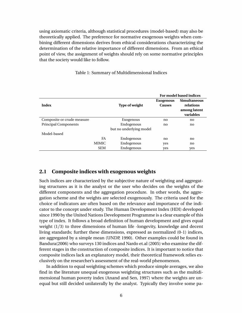
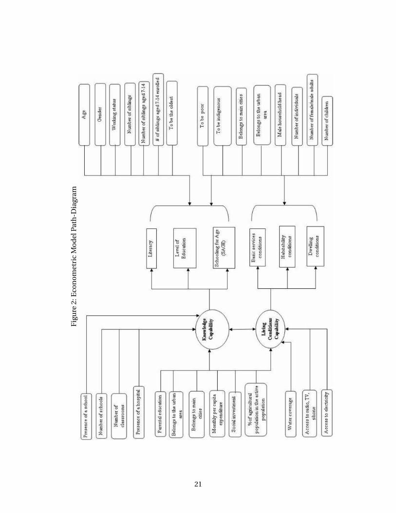
In this section we illustrate the use of the preceding measures to analyze the depri-vation situation of Bolivia’s children in the capability domains of knowledge and liv-ing conditions. The deprivation measures are applied to the estimated factor scoresof the latent variable model proposed by Krishnakumar and Ballon (2008). The dataused in this model corresponds to the 2002 MECOVI program, a National HouseholdSurvey conducted by the National Statistical Institute of Bolivia, with the support ofthe World Bank. The 2002 survey covers 5,952 households and 24,933 individualsand contains information at the national and regional levels, on education, health,migration, labor, income, household characteristics, and living conditions. The in-formation of the MECOVI 2002 survey is complemented with information from theNational Institute of Statistics (INE) on social investment and school conditions atthe municipal level for data on some exogenous variables of our model. Our samplecomprises 5313 enrolled primary school children aged 7-14. Figure 2 presents path-diagram of the econometric model used to operationalize the capability theory tothe Bolivian case.
As shown by the path-diagram, knowledge and living conditions capabilities,represented by circles, are measured by three functioning indicators in each case.The indicators for educational achievements include literacy, level of education, andschooling for age (SAGE). The SAGE variable reflects the lag in a child’s schoolingwith reference to a ’normal’ achievement rate (see, Psacharopoulos and Yand, 1991).A score under 1 is considered as being below normal progress in the school systembecause of late entry or dropping out and/or re-enrollment and the further awayit is below 1 the lower the performance of the child. Living conditions outcomesare measured by the quality of basic services, and the quality of dwelling and hab-itability conditions enjoyed by the household. These three indicators are measured
19
by an ordered categorical variable with three categories indicating low, middle, andhigh quality. The exogenous variables included in the structural and measurementequations (1) and (2), respectively are split into supply and demand factors. Theseare classified according to their influential role in the enhancement of capabilities,and in the choice process. Thus, supply variables (number of schools, number ofclassrooms, parental education, etc) are included in the structural equations, anddemand variables (age, gender, indigenous status, etc.) in the measurement equa-tions. In the path-diagram these are represented on the left and right hand side,respectively.
20
Fig
ure
2:E
con
om
etri
cM
od
elPa
th-D
iagr
am
21
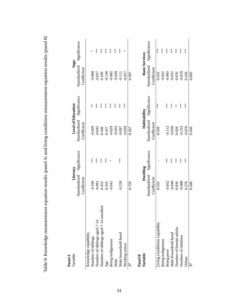
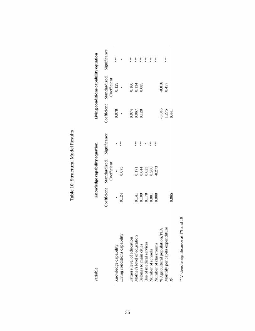
Tables 9 and 10 of the appendix present the estimated parameters of the econo-metric model described by the path-diagram. We will not discuss them in detailhere, as our main concern is the deprivation situation. The reader is referred toKrishnakumar and Ballon (2008) for a detailed interpretation of the results. Brieflyspeaking, we see that there is a positive simultaneous relationship between knowl-edge and living conditions capabilities implying that they mutually enhance eachother. The structural equation results also show that parental education, and supplyvariables of health and education access, along with, urban location have a positiveinfluence in the enhancement of both capability sets. Regarding the measurementequations, we observe a positive loading for each of the capability domains on itscorresponding indicators. Among the exogenous variables included in these equa-tions we see that being indigenous or poor has a negative effect on the achievedfunctionings in both dimensions given the same capability level. The sibling struc-ture and working status have a mixed and negative effects on educational achieve-ments, respectively. Urban environment seems to favour better housing conditions.
Computing the CDI’s
On the basis of the estimated parameters and the estimated factor scores (obtainedas explained in section 3), we compute the capability deprivation indices presentedin section 4. We only look at 14-year old children as it is only or this age group thatone can talk of not being able to achieve a minimal functioning level. Our analy-sis is carried out for 14-year-old children belonging to one of the following groups:female/rural, female/urban, male/rural and male/urban. We only consider 14 year-old children because it is only at this age that one can define an absolute criteria foridentifying the capability deprived in the knowledge domain as they are expected tohave finished primary education at this age. For these children, we fix the minimallevel of (threshold) educational functionings corresponding to the ‘fictitious’ childat the threshold deprivation level as being literate (if we fix it as illiterate, we end upwith too few deprived)12, a SAGE (lag in schooling progress) value of 0.5 and with in-complete primary education. The living conditions threshold is represented by thesame fictitious child living in a house with a ‘low’ quality of basic services, habit-ability, and dwelling conditions. Along with these characteristics of the indicators,we also need to fix the exogenous variables in our model for calculating the thresh-old deprivation level. As these exogenous factors influence the choice process andthe capability set, we propose to fix them at their minimum or maximum observedvalue depending on whether the associated coefficient is positive or negative (Ta-bles 7 and 8 of the appendix). Thus the fictitious deprived child (representing thethreshold of deprivation) will be surrounded by the most unfavorable environment.Table 2 presents the conditions characterizing the deprivation threshold.
Once the model is estimated, we compute the scores (representing the capabili-ties) for all individuals in each dimension. In order to calculate the ranks of the in-
12The issue of where to fix the minimum level of achievement for the threshold is a crucial one asthe results are obviously sensitive to the value chosen; we will say more about this problem whileexamining the results.
22
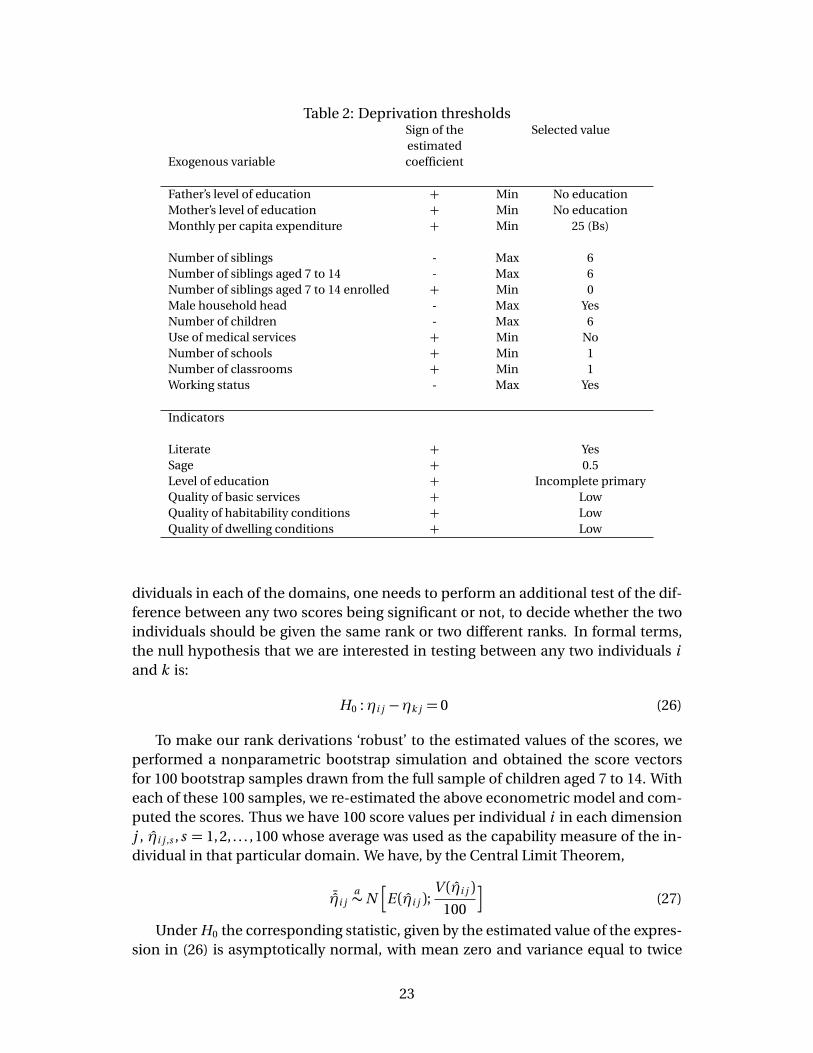
Table 2: Deprivation thresholdsSign of the Selected valueestimated
Exogenous variable coefficient
Father’s level of education + Min No educationMother’s level of education + Min No educationMonthly per capita expenditure + Min 25 (Bs)
Number of siblings - Max 6Number of siblings aged 7 to 14 - Max 6Number of siblings aged 7 to 14 enrolled + Min 0Male household head - Max YesNumber of children - Max 6Use of medical services + Min NoNumber of schools + Min 1Number of classrooms + Min 1Working status - Max Yes
Indicators
Literate + YesSage + 0.5Level of education + Incomplete primaryQuality of basic services + LowQuality of habitability conditions + LowQuality of dwelling conditions + Low
dividuals in each of the domains, one needs to perform an additional test of the dif-ference between any two scores being significant or not, to decide whether the twoindividuals should be given the same rank or two different ranks. In formal terms,the null hypothesis that we are interested in testing between any two individuals iand k is:
H0 :ηi j −ηk j = 0 (26)
To make our rank derivations ‘robust’ to the estimated values of the scores, weperformed a nonparametric bootstrap simulation and obtained the score vectorsfor 100 bootstrap samples drawn from the full sample of children aged 7 to 14. Witheach of these 100 samples, we re-estimated the above econometric model and com-puted the scores. Thus we have 100 score values per individual i in each dimensionj , η̂i j ,s ,s = 1, 2, . . . , 100 whose average was used as the capability measure of the in-dividual in that particular domain. We have, by the Central Limit Theorem,
¯̂ηi ja∼N
hE (η̂i j );
V (η̂i j )100
i(27)
Under H0 the corresponding statistic, given by the estimated value of the expres-sion in (26) is asymptotically normal, with mean zero and variance equal to twice
23
the variance given in (27) as we assume that individuals are independent and themoments of the distribution of latent factors are invariant over individuals. If H0 isrejected, i and k will be assigned two different ranks.
Given that the factor scores are continuous latent variables, and because of theirimplications on the well-being status of the individuals, our ranking algorithm basedon the above hypothesis testing procedure must be reluctant to accept the equal-ity of two factor scores leading to identical rankings. That means that in our case,the Type II error is more important than the Type I error, as assigning equal ranksbetween two individuals implies that their well-being status is the same. Thus wedecided to minimize the Type II error by reducing the null hypothesis region of ac-ceptance to a 5% interval.
The following tables report our capability deprivation indices for the four groups.Panel A of Table 3 describes the within deprivation indices in the knowledge domain.Comparing urban and rural groups, we see that the head count ratio (i.e. the propor-tion of deprived children) is higher among the rural population, with a bigger differ-ence among males compared to females. This means that 67% of rural females, 73%of rural males, 47% of urban males, and 49% of urban females do not enjoy the abilityto achieve minimal functionings in knowledge capability. Regarding the the inten-sity of deprivation given by our per capita deprivation (rank) gap (CDI), once again,we see that it is higher in rural areas for both males and females, with a greater gapdifference among males (16 per capita positions compared to 9 in the female case).We can therefore say that living in urban areas provides a bigger choice range andmore so for male children than the female ones.
In what follows we will be looking at some descriptive statistics regarding theachievement indicators and exogenous variables of the deprived children in eachof these groups (see Tables 4, 5 and 6). Perhaps it is necessary to explain why itis useful to look at these statistics. As mentioned earlier, the capability depriva-tion threshold was calculated by fixing the achievements at at a ’minimal’ level andthe exogenous factors at their most unfavourable state. The resulting deprivationthreshold is an endogenous combination of all this information coming out of themodel. Then we determine the ’deprived’ children as those being below the thresh-old thus derived. But this does not necessarily mean that they will all be below theminimal/least favourable level in all the functionings and exogenous variables. Thatis why we compute these descriptives to see which indicators/exogenous variablesseem to influence deprivation the most.
Looking at Table 4 presenting the distribution of ‘knowledge’ deprived childrenamong the three achievement indicators, we see that level of education is the mostconstraining component with 98% of children exhibiting incomplete primary edu-cation, in rural regions, and 96% in urban areas. 13 It is interesting to note that theaverage value of SAGE for ’knowledge’ deprived children is between 0.6 and 0.7 units
13The Literacy column is not very informative as they are all literate, which is logical according tothe minimum we fixed for this indicator.
24
i.e. above the level corresponding to the fictitious deprived child (0.5) though nottoo far from it.
From Table 5 we find that parental education is low among ‘knowledge’ deprivedchildren, with high proportion of parents exhibiting incomplete primary (even thoughthe threshold taken was ’no education’ there are more in ’incomplete primary thanin ’no education’ except for the female urban group). This situation worsens in thecase of female children. Regarding other exogenous variables (see Table 6) we findthat the use of medical services is also low in all the four groups with values rang-ing between 10 to 16% among rural and urban females, respectively, and 11% and12% among their peer males. Finally, we see that working status is higher amongthe rural groups. Though, the deprived children indeed face a disadvantageous mi-lieu, it is less restrictive compared to that of our fictitious child. The above analysisis also useful to identify the aspects that need the most attention for improving thecapability status of children in the knowledge domain.
Turning to living conditions capability, Panel B of Table 3, we note that the per-centage of deprived individuals and the intensity of their deprivation are higheramong rural groups in this case too. However, the differences between females andmales by region are less important for both the head count and the CDI. The headcount ratio is between 2 to 6% in the female group and between 3 to 6% in the maleone. The per capita deprivation gap is around 1 position in each of the four groups.Thus it seems that the situation is much better for living conditions than for knowl-edge capability. However, the small values of these measures need to be interpretedwith caution as the threshold positions in both dimensions are not strictly compara-ble. Recall that the fictitious deprived child in this case is one exhibiting low qualityin all the indicators relating to basic services, habitability and dwelling conditions,which really depict the bare minimum and rather desperate conditions of living.
Our explanation for the low index values here is that the threshold itself being solow the percentage of population below this level and the intensity of deprivation arevery small. We come back to our earlier remark about the sensitivity of the index tothe choice of the threshold level which is clear in this case. The values would be reallydifferent (and much bigger) if we had chosen ’medium’ quality for the minimumachievement level. It is our intention to explore this issue further in future work.
Our explanation is supported by the comparison between the two sets of de-prived (’knowledge’ deprived and ’living conditions’ deprived) in terms of descrip-tive statistics relating to exogenous variables (see Tabes 5 and 6). All the variablessuch as parental education level, average monthly per capita expenditure, use ofmedical services are much lower for the ’living conditions’ deprived.
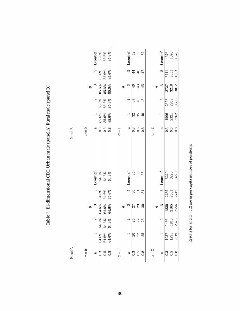
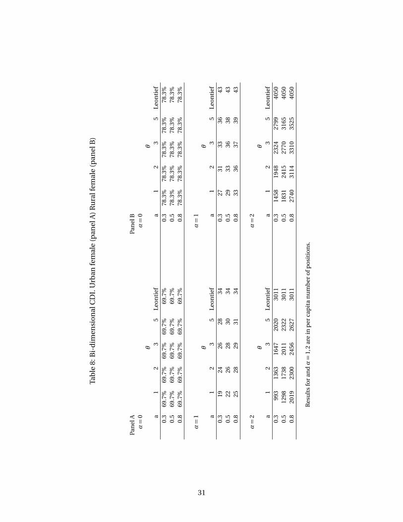
Deprivation in the bi-dimensional space is reported in Table 7 for the male groups,and in Table 8 for the female groups. The first column of both tables, labelled ’a’, isthe weight assigned to the living conditions dimension. The substitution param-eter (θ ) ranges from perfect substitution (one) to no substitution (Leontief). Thealpha values correspond to the head count ratio (union approach, α = 0), the bi-dimensional deprivation intensity per capita gap (α = 1), and the bi-dimensionaldeprivation severity per capita gap (α = 2). Comparing urban and rural male chil-dren (Table 7) we observe that for the three deprivation measures, the deprivation
25
status of rural males is higher than that of urban males. The head count ratio ishigher by 21%, and the per capita intensity measure is between 12 to 16 positionshigher. Looking at the weights, we see that as the weight attached to living condi-tions increases (from 0.3 to 0.8) the intensity and severity measures also increase. Inaddition, we observe that as the degree of substitution decreases the intensity andthe severity measures increase for all weights. This is in accordance with the notionsof substitution and complementarity underlying the CES functional form. As θ in-creases it becomes more difficult to compensate one dimensional deprivation withanother. This is related to the ’nature’ of the dimensions: whenever they reflect verydifferent aspects of life, it seems reasonable to assume low degree of substitution. Inour analysis we have considered a range of possibilities (one to Leontief) although,we think that no substitution (Leontief) is more reasonable to assume in the case ofliving conditions and education. The results for female groups (Table 8) show a sim-ilar pattern regarding the proportion of deprived, and the bi-dimensional intensityand severity measures, for all weights. However, the differences between rural andurban female groups are much smaller compared to males. This is also true for theno substitution case. We see that these measures increase as the degree of substi-tution decreases. As in the single dimensional case we evidence that living in urbanareas has an enhancing effect on the choice set of male children.
26
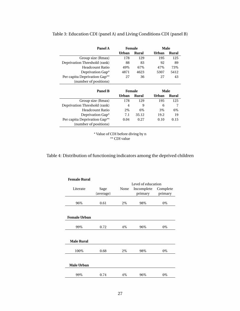
Table 3: Education CDI (panel A) and Living Conditions CDI (panel B)
Panel A Female MaleUrban Rural Urban Rural
Group size (Rmax) 178 129 195 125Deprivation Threshold (rank) 88 83 92 89
Headcount Ratio 49% 67% 47% 73%Deprivation Gap* 4871 4623 5307 5412
Per capita Deprivation Gap** 27 36 27 43(number of positions)
Panel B Female MaleUrban Rural Urban Rural
Group size (Rmax) 178 129 195 125Deprivation Threshold (rank) 4 9 6 7
Headcount Ratio 2% 6% 3% 6%Deprivation Gap* 7.1 35.12 19.2 19
Per capita Deprivation Gap** 0.04 0.27 0.10 0.15(number of positions)
* Value of CDI before diving by n** CDI value
Table 4: Distribution of functioning indicators among the deprived children
Female RuralLevel of education
Literate Sage None Incomplete Complete(average) primary primary
96% 0.61 2% 98% 0%
Female Urban
99% 0.72 4% 96% 0%
Male Rural
100% 0.68 2% 98% 0%
Male Urban
99% 0.74 4% 96% 0%
27
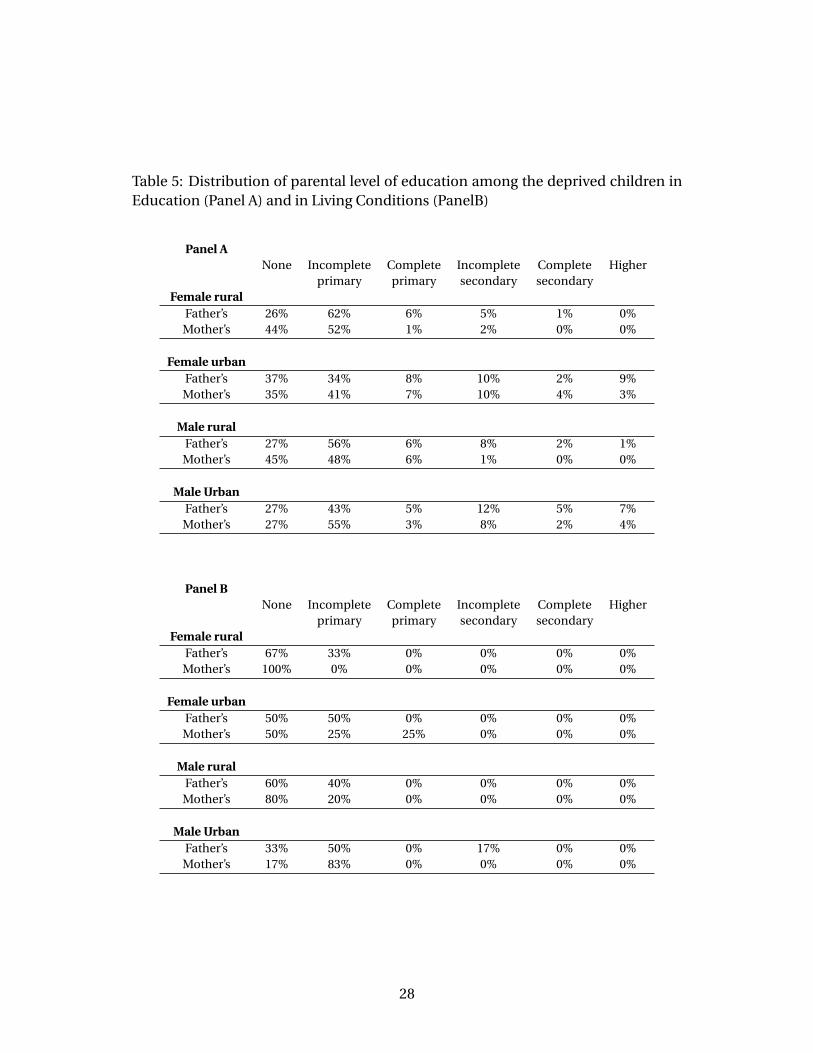
Table 5: Distribution of parental level of education among the deprived children inEducation (Panel A) and in Living Conditions (PanelB)
Panel ANone Incomplete Complete Incomplete Complete Higher
primary primary secondary secondaryFemale rural
Father’s 26% 62% 6% 5% 1% 0%Mother’s 44% 52% 1% 2% 0% 0%
Female urbanFather’s 37% 34% 8% 10% 2% 9%Mother’s 35% 41% 7% 10% 4% 3%
Male ruralFather’s 27% 56% 6% 8% 2% 1%Mother’s 45% 48% 6% 1% 0% 0%
Male UrbanFather’s 27% 43% 5% 12% 5% 7%Mother’s 27% 55% 3% 8% 2% 4%
Panel BNone Incomplete Complete Incomplete Complete Higher
primary primary secondary secondaryFemale rural
Father’s 67% 33% 0% 0% 0% 0%Mother’s 100% 0% 0% 0% 0% 0%
Female urbanFather’s 50% 50% 0% 0% 0% 0%Mother’s 50% 25% 25% 0% 0% 0%
Male ruralFather’s 60% 40% 0% 0% 0% 0%Mother’s 80% 20% 0% 0% 0% 0%
Male UrbanFather’s 33% 50% 0% 17% 0% 0%Mother’s 17% 83% 0% 0% 0% 0%
28
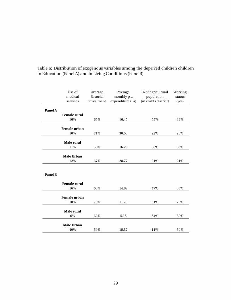
Table 6: Distribution of exogenous variables among the deprived children childrenin Education (Panel A) and in Living Conditions (PanelB)
Use of Average Average % of Agricultural Workingmedical % social monthly p.c. population statusservices investment expenditure (Bs) (in child’s district) (yes)
Panel AFemale rural
16% 65% 16.45 55% 34%
Female urban10% 71% 30.53 22% 28%
Male rural11% 58% 16.20 56% 53%
Male Urban12% 67% 28.77 21% 21%
Panel B
Female rural16% 63% 14.89 47% 33%
Female urban18% 79% 11.79 31% 75%
Male rural0% 62% 5.15 54% 60%
Male Urban40% 59% 15.57 11% 50%
29
Tab
le7:
Bi-
dim
ensi
on
alC
DI.
Urb
anm
ale
(pan
elA
)R
ura
lmal
e(p
anel
B)
Pan
elA
Pan
elB
α=
0α=
0θ
θa
12
35
Leo
nti
efa
12
35
Leo
nti
ef0.
364
.6%
64.6
%64
.6%
64.6
%64
.6%
0.3
85.6
%85
.6%
85.6
%85
.6%
85.6
%0.
564
.6%
64.6
%64
.6%
64.6
%64
.6%
0.5
85.6
%85
.6%
85.6
%85
.6%
85.6
%0.
864
.6%
64.6
%64
.6%
64.6
%64
.6%
0.8
85.6
%85
.6%
85.6
%85
.6%
85.6
%
α=
1α=
1θ
θa
12
35
Leo
nti
efa
12
35
Leo
nti
ef0.
320
2527
3035
0.3
3237
4044
520.
522
2729
3135
0.5
3540
4346
520.
825
2830
3135
0.8
4043
4547
52
α=
2α=
2θ
θa
12
35
Leo
nti
efa
12
35
Leo
nti
ef0.
310
2714
9318
3022
3532
200.
319
0623
5327
2732
4146
760.
512
9118
4621
6525
0332
200.
523
2128
5332
1836
5146
760.
820
1923
7525
5627
4932
200.
832
6236
0338
1240
5346
76
Res
ult
sfo
ran
dα=
1,2
are
inp
erca
pit
an
um
ber
ofp
osi
tio
ns.
30
Tab
le8:
Bi-
dim
ensi
on
alC
DI.
Urb
anfe
mal
e(p
anel
A)
Ru
ralf
emal
e(p
anel
B)
Pan
elA
Pan
elB
α=
0α=
0θ
θa
12
35
Leo
nti
efa
12
35
Leo
nti
ef0.
369
.7%
69.7
%69
.7%
69.7
%69
.7%
0.3
78.3
%78
.3%
78.3
%78
.3%
78.3
%0.
569
.7%
69.7
%69
.7%
69.7
%69
.7%
0.5
78.3
%78
.3%
78.3
%78
.3%
78.3
%0.
869
.7%
69.7
%69
.7%
69.7
%69
.7%
0.8
78.3
%78
.3%
78.3
%78
.3%
78.3
%
α=
1α=
1θ
θa
12
35
Leo
nti
efa
12
35
Leo
nti
ef0.
319
2426
2834
0.3
2731
3336
430.
522
2628
3034
0.5
2933
3638
430.
825
2829
3134
0.8
3336
3739
43
α=
2α=
2θ
θa
12
35
Leo
nti
efa
12
35
Leo
nti
ef0.
399
313
6316
4720
2030
110.
314
5819
4823
2427
9940
500.
512
9817
3820
1123
2230
110.
518
3124
1527
7031
6540
500.
820
1923
0024
5626
2730
110.
827
4031
1433
1035
2540
50
Res
ult
sfo
ran
dα=
1,2
are
inp
erca
pit
an
um
ber
ofp
osi
tio
ns.
31
6 Conclusions
In this paper we propose a capability deprivation index that is based on scores de-rived from a structural economic model explaining the different capabilities usingexogenous (social, economic, institutional) causes. We specify the freedom of choicegiven by any capability set as a latent variable partially observed through a vector offunctioning indicators, and influenced by a collection of exogenous variables. Thus,our model measures deprivation in the functioning-capability space. The estimatorof the latent variable vector, or factor scores, provides us with a measure of the well-being status of the individuals in the different dimensions. We propose an indexthat only uses the ordinal information (ranks) for defining the deprivation status in-cluding the quantitative information for defining weights. We distinguish two typesof indices, one regarding deprivation within a capability set, and one consideringaggregation across capability sets. That is, our index belongs to a class of multipledimension(capabilities)- multiple indicator(functionings) indices. Both types of in-dices fulfill a set of desirable properties in the capability framework.
We applied our indices to analyze capability deprivation in the knowledge andliving conditions of Bolivia’s children in 2002. We differentiated four groups accord-ing to their gender and urban/rural location. Looking at individual dimensions, wefind urban environment seems to enhance the choice set and more so for males inthe knowledge dimension. The situation is similar for the living conditions domainthough the difference between males and females is much less pronounced.
The bi-dimensional measures show the importance of living conditions in theoverall deprivation as the deprivation measures tend to increase when their associ-ated weight increases. They are also sensitive to the degree of substitution betweendimensions, showing greater values, as the degree of substitution decreases. Finally,from the policy angle, it is interesting to note the role played by the exogenous vari-ables in the CDI. The supply and demand factors, especially parental education,and the use of health services, largely account for how individuals turn out to bedeprived. This highlights their importance as policy instruments for targeting themost deprived.
An important issue which needs to be explored and which we have not done inthis paper is the choice of the minimum levels of achievement for determining thedeprivation threshold, as we have used absolute criteria for identifying the deprived.It is clear that the results are sensitive to the criteria, and in order to make ‘robust’conclusions, further investigations are needed.
32

7 Appendices
33
Tab
le9:
Kn
owle
dge
mea
sure
men
teq
uat
ion
resu
lts
(pan
elA
)an
dli
vin
gco
nd
itio
ns
mea
sure
men
teq
uat
ion
resu
lts
(pan
elB
)
Pan
elA
Var
iab
leL
iter
acy
Lev
elo
fEd
uca
tio
nSa
geSt
and
ard
ized
Sign
ifica
nce
Stan
dar
diz
edSi
gnifi
can
ceSt
and
ard
ized
Sign
ifica
nce
Co
effi
cien
tC
oef
fici
ent
Co
effi
cien
tK
now
led
geca
pab
ilit
yN
um
ber
ofs
ibli
ngs
-0.1
06**
*-0
.029
**-0
.068
*N
um
ber
ofs
ibli
ngs
aged
7-14
-0.0
91**
*-0
.045
***
-0.0
27**
*N
um
ber
ofs
ibli
ngs
aged
7-14
enro
lled
0.45
3**
*0.
166
***
0.18
9**
*A
ge0.
534
***
0.44
7**
*-0
.156
***
Bei
ng
ind
igen
ou
s-0
.041
*-0
.029
***
-0.0
82**
*M
ale
-0.0
33**
*-0
.028
***
Mal
eh
ou
seh
old
hea
d-0
.228
***
-0.0
97**
*-0
.111
***
Wo
rkin
gst
atu
s-0
.039
***
-0.0
17*
R2
0.75
90.
567
0.50
7
Pan
elB
Vari
able
Dw
elli
ng
Hab
itab
ilit
yB
asic
Serv
ices
Stan
dar
diz
edSi
gnifi
can
ceSt
and
ard
ized
Sign
ifica
nce
Stan
dar
diz
edSi
gnifi
can
ceC
oef
fici
ent
Co
effi
cien
tC
oef
fici
ent
Livi
ng
con
dit
ion
sca
pab
ilit
y0.
532
-0.
546
***
0.53
2**
*B
ein
gin
dig
eno
us
-0.0
31**
*B
ein
gp
oo
r-0
.052
***
-0.1
12**
*-0
.065
***
Mal
eh
ou
seh
old
hea
d-0
.048
***
-0.0
50**
*-0
.031
***
Nu
mb
ero
ffem
ale
adu
lts
0.03
6**
*0.
028
**0.
076
***
Nu
mb
ero
fch
ild
ren
-0.0
80**
*-0
.233
***
-0.0
78**
*U
rban
0.27
8**
*-0
.076
***
0.43
6**
*R
20.
500
0.44
60.
695
34
Tab
le10
:Str
uct
ura
lMo
del
Res
ult
s
Var
iab
leK
now
led
geca
pab
ilit
yeq
uat
ion
Liv
ing
con
dit
ion
sca
pab
ilit
yeq
uat
ion
Co
effi
cien
tSt
and
ard
ized
.Si
gnifi
can
ceC
oef
fici
ent
Stan
dar
diz
ed.
Sign
ifica
nce
Co
effi
cien
tC
oef
fici
ent
Kn
owle
dge
cap
abil
ity
--
-0.
078
0.12
9**
*Li
vin
gco
nd
itio
ns
cap
abil
ity
0.12
40.
075
***
--
-
Fath
er’s
leve
lofe
du
cati
on
0.07
40.
160
***
Mo
ther
’sle
velo
fed
uca
tio
n0.
141
0.17
1**
*0.
067
0.13
4**
*B
elo
ngs
tom
ain
citi
es0.
109
0.04
4**
*0.
128
0.08
5**
*U
seo
fmed
ical
serv
ices
0.17
00.
023
***
*N
um
ber
ofs
cho
ols
0.00
10.
200
***
***
Nu
mb
ero
fcla
ssro
om
s0.
000
-0.2
73**
***
*%
Agr
icu
ltu
ralp
op
ula
tio
n/P
EA
-0.0
45-0
.016
Mo
nth
lyp
erca
pit
aex
pen
dit
ure
1.27
50.
457
***
R2
0.06
50.
441
***,
*d
eno
tesi
gnifi
can
ceat
1%an
d10
35
References
Bollen, K. (1989). Structural Equations with Latent Variables. Jhon Wiley and Sons,New York.
Bourguignon, F. and S. Chakravarty (1999). A family of multidimensional povertymeasures. In: Advances in Econometrics, Income Distribution and Methodologyof Science (D.,Slottje, Eds.). Physica-Verlag, London.
Bourguignon, F. and S. Chakravarty (2002). Multi-dimensional poverty orderings.Working Paper No. 2002-22, Delta, Paris.
Bourguignon, F. and S. Chakravarty (2003). The measurement of multidimensionalpoverty. Journal of Economic Inequality 1(1), 25–49.
Chambers, R. (1994). The origins and practice of participatory rural appraisal. WorldDevelopment 22(7), 953–969.
Clert, C. (1999). Evaluating the concept of social exclusion in development discourse.European Journal of Development Research 11(2), 176–199.
European-Foundation (1995). Public Welfare Services and Social Exclusion: The De-velopment of Consumer Oriented Initiatives in the European Union. The Euro-pean Foundation, Dublin.
Krishnakumar, J. (2007). Going beyond functionings to capabilities: An economet-ric model to explain and estimate capabilities. Journal of Human Development8(1), 39–63.
Krishnakumar, J. and A. Nagar (2008). On exact statistical properties of multidi-mensional indices based on principal components, factor analysis, mimic andstructural equation models. Social Indicators Research 86(3), 481–496.
Krishnakumar, J. and P. Ballon (2008). Estimating basic capabilities: A structuralequation model applied to bolivia. World Development 36(6), 992–1009.
Maasoumi, E. and M. Lugo (2008). The information basis of multivariate poverty as-sessments. In: Quantitative Approaches to Multidimensional Poverty Measure-ment (Kakwani, N. and Silber, J., Ed.). Palgrave-MacMillan.
Muthen, B.O. (2002). Beyond sem: General latent variable modelling. Behav-iormetrika 29(1), 81–117.
Sen, A. K. (1983). Poor, relatively speaking. Oxford Economic Papers 35(2), 153–69.
Skrondal, A. and S. Rabe-Hesketh (2004). Generalized Latent Variable Modeling:Multilevel, Longitudinal, and Structural Equation Models. Chapman Hall, BocaRaton, USA.
36
Townsend, P. (1979). Poverty in the United Kingdom: A Survey of HouseholdRessources and Standard of Living. University of California Press, Berkley.
Tsui, K. (2002). Multidimensional poverty indices. Social Choice and Welfare19(1), 69–93.
Zheng, B. (1997). Aggregate poverty measures. Journal Economic Surveys 11(2), 123–162.
37