A meshless method based on moving least squares … · A meshless method based on moving least squares for the simulation of free ... HAN1 (1College of Shipbuilding Engineering,

Lu et al. / J Zhejiang Univ-Sci A (Appl Phys & Eng) 2016 17(2):130-143 130

A meshless method based on moving least squares for the

simulation of free surface flows*

Yu LU†1, An-kang HU1,2, Ya-chong LIU1, Chao-shuai HAN1 (1College of Shipbuilding Engineering, Harbin Engineering University, Harbin 150001, China)

(2CIMC Ocean Engineering Design & Research Institute Co., Ltd., Shanghai 201206, China) †E-mail: [email protected]

Received Mar. 15, 2015; Revision accepted Sept. 18, 2015; Crosschecked Dec. 16, 2015

Abstract: In this paper, a meshless method based on moving least squares (MLS) is presented to simulate free surface flows. It is a Lagrangian particle scheme wherein the fluid domain is discretized by a finite number of particles or pointset; therefore, this meshless technique is also called the finite pointset method (FPM). FPM is a numerical approach to solving the incompress-ible Navier–Stokes equations by applying the projection method. The spatial derivatives appearing in the governing equations of fluid flow are obtained using MLS approximants. The pressure Poisson equation with Neumann boundary condition is handled by an iterative scheme known as the stabilized bi-conjugate gradient method. Three types of benchmark numerical tests, namely, dam-breaking flows, solitary wave propagation, and liquid sloshing of tanks, are adopted to test the accuracy and performance of the proposed meshless approach. The results show that the FPM based on MLS is able to simulate complex free surface flows more efficiently and accurately. Key words: Meshless method, Moving least squares (MLS), Free surface flows, Finite pointset method (FPM), Dam-breaking

flows, Solitary wave propagation, Liquid sloshing of tanks http://dx.doi.org/10.1631/jzus.A1500053 CLC number: U661.1

1 Introduction

Recently, meshless methods are playing a new role in providing a promising and capable alternative in the general area of numerical simulations of free surface flows, which can be advantageous, particu-larly in cases wherein meshing (Dumbser, 2013) and remeshing would be computationally elaborate.

Meshless methods as Lagrangian particle schemes typically only have points as computational instances. Automatically, the boundaries of the com-putational domain are defined in the manner of up-

dating the positions of calculated particles. Com-pared with the Eulerian methods that need strict top-ological meshes that consume time and present simulation difficulty in terms of the large defor-mation or intricated geometries, the Lagrangian par-ticle methods wherein the distribution of particles can be quite arbitrary are found to be appropriate and acceptable for solving fluid flow with moving free surface (Lu et al., 2015).

Among the various meshless methods, smoothed-particle hydrodynamics (SPH) is the most classical and famous Lagrangian particle method for flow-governing equations. Originally invented to solve astrophysical simulations without boundary (Gingold and Monaghan, 1977; Lucy, 1977), the method has been further generalized to many other types of flows and applications, such as the dynamic response of elastoplastic materials (Libersky et al., 1993;

* Project supported by the National Natural Science Foundation of China (Nos. 51379040 and 51409063)

ORCID: Yu LU, http://orcid.org/0000-0001-7859-2876 © Zhejiang University and Springer-Verlag Berlin Heidelberg 2016

Journal of Zhejiang University-SCIENCE A (Applied Physics & Engineering)

ISSN 1673-565X (Print); ISSN 1862-1775 (Online)

www.zju.edu.cn/jzus; www.springerlink.com

E-mail: [email protected]


Benz and Asphaug, 1995; Song et al., 2006), solid friction (Maveyraud et al., 1999), heat transfer (Cleary and Monaghan, 1999), turbulence modeling (Monaghan, 2002), multiphase flows (Monaghan and Kocharyan, 1995; Morris, 2000), free surface flows (Monaghan, 1994), viscoelastic flows (Ellero et al., 2002; Fang et al., 2006), viscous flows (Flebbe et al., 1994; Takeda et al., 1994; Watkins et al., 1996; Morris et al., 1997), incompressible fluids (Cummins and Rudman, 1999; Shao and Lo, 2003), and geophysical flows (Oger and Savage, 1999; Cleary and Prakash, 2004; Ata and Soulaïmani, 2005). However, some numerical defects plague the SPH method, including inconsistency, low accuracy, and the incorporation of boundary conditions. Sever-al methods on the improved SPH algorithm can be found in Ferrari et al. (2008; 2009).

One of the generations of meshless method is the finite pointset method (FPM), in which the gov-erning equations are approximated in their differen-tial (strong) form using meshless finite difference approximations. This Lagrangian particle method was proposed by Oñate et al. (1996a; 1996b), which has been further developed for fluid mechanics prob-lems. FPM adopts moving least squares (MLS) (Be-lytschko et al., 1996; Deshpande et al., 1998; Dilts, 1999) for reconstructing a function from values giv-en at a finite number of scattered data particles (pointset), which move with fluid velocity and carry all information necessary for solving fluid dynamic quantities and discretizing fluid dynamic equations. Thereupon, this method makes it more natural in the case of numerical implementation as well as more flexible for the boundary conditions treatment and particle management. FPM has been efficiently used for solving a wide range of fluid flow problems (Oñate and Idelsohn, 1998; Oñate et al., 2000; Löh-ner et al., 2002).

In this paper, the FPM for numerical simulation of free surface flows is presented. The incompressi-ble Navier–Stokes equations are taken care of by the widely used projection method (Chorin, 1968), re-sulting in the resolution of Poisson problems at each time step. Therefore, the MLS method is obtained to approximate the spatial derivatives appearing in the pressure Poisson equation. To satisfy the boundary condition, we use this method by placing the bound-

ary particles at all domain boundaries. For the free surface treatment, a criterion of the particle density is used to detect the free surface particles over time steps. Three typical problems associated with free surface flows involving dam-breaking flows, solitary wave propagation, and liquid sloshing of tanks are solved to demonstrate that the proposed FPM can accurately and efficiently simulate complex free sur-face flow problems.

In this paper, the theory of FPM is examined first, which mainly includes the mathematical model, the projection method, the MLS method and its ex-tension to solving the pressure Poisson equation, and the free surface treatment, presented in Section 2. Then, the numerical tests with the corresponding results are presented in Section 3. Finally, some con-cluding remarks are presented. 2 Numerical methodology of FPM

2.1 Mathematical model

The incompressible Navier–Stokes equations in the Lagrangian form can be written as follows:

DD0,

D Di

i

u

t x

(1)

D,

Di i

ii i j

u upf

t x x x

(2)

where ρ is the fluid density, t is the time, ui is the ith Cartesian component of the velocity field, xi is the ith Cartesian component of the position vector, p is the pressure, μ is the viscosity, and fi is the source term (normally, the gravity acceleration g). Dφ/Dt denotes the total or material time derivative of a function φ.

2.2 Projection method

The projection method is adopted for solving Eqs. (1) and (2) in FPM. It consists of two fractional steps. The momentum conservation Eq. (2) is explic-itly solved to compute the new particle position and

the temporal velocity 1niu at the first step:

1 ,n n n

i i ir r tu (3)


1 ,n

n n ii i i

i j

uu u t tf

x x

(4)

where nir is the Cartesian ith components of the parti-

cle position vector.

Secondly, 1niu is corrected by the equation

1

+1 1 ,n

n ni i

i

t pu u

x

(5)

where the pressure gradient is added. Meantime, the

resultant velocity +1niu should meet the incompressi-

bility condition

1

0.ni

i

u

x

(6)

The pressure pn+1 is solved implicitly by the fol-

lowing pressure Poisson equation derived from Eqs. (5) and (6):

11

.nni

i i i

up

x x t x

(7)

Consider the condition on boundary Γ, where

the corresponding boundary particles will remain in their positions, the velocity of which can be ex-pressed as

0, 0 and 0,t t

u

n u nn

(8)

where u is the velocity vector and n is the unit nor-mal vector. The pressure boundary condition is ac-quired by projecting Eq. (5) on the outward unit normal vector n to the boundary Γ. Thus, the pres-sure Neumann boundary condition is written as

1

D( ) ( ).

D

np u

f ut

n n nn

(9)

In the projection method, the particle positions

change only in the first step. The intermediate veloc-ity, the pressure, and the final divergence free veloci-ty are all computed on the new particle positions.

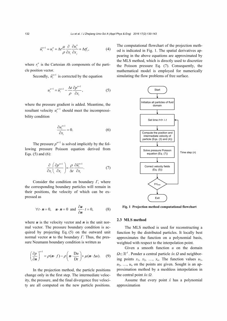
The computational flowchart of the projection meth-od is indicated in Fig. 1. The spatial derivatives ap-pearing in the above equations are approximated by the MLS method, which is directly used to discretize the Poisson pressure Eq. (7). Consequently, the mathematical model is employed for numerically simulating the flow problems of free surface.

2.3 MLS method

The MLS method is used for reconstructing a function by the distributed particles. It locally best approximates the function on a polynomial basis, weighted with respect to the interpolation point.

Given a smooth function u on the domain

Ω d . Ponder a central particle xΩ and neighbor-ing points x1, x2, …, xn. The function values u1, u2, …, un on the points are given. Sought is an ap-proximation method by a meshless interpolation in the central point xΩ.

Assume that every point x has a polynomial approximation

Fig. 1 Projection method computational flowchart

Compute the position and intermediate velocity of

particle (Eqs. (3) and (4))

t>tmax

Exit

Start

Set time t=t+Δt

Initialize all particles of fluid domain

Solve pressure Poisson equation (Eq. (7))

Correct velocity fields (Eq. (5))

Time step (n)


T

0

( ) ( )= ( ) ( ) ( ),k

j jj

u x p x a b x x x

b a (10)

where the operator Π on u equates the function p(x), which is formulated in polynomial form by the con-struction of the neighboring data particles x1, x2, …,

xn. T

0 1( )=[ ( ), ( ), ..., ( )]kx a x a x a xa denotes the coeffi-

cient vector and T0 1( )=[ ( ), ( ), ..., ( )]kx b x b x b xb is the

basis vector. In this study, a canonical basis in two dimensions is

0 1 2( , ) 1, ( , ) , ( , ) ,b x y b x y x b x y y 2 2

3 4 5( , ) , ( , ) , ( , ) ,b x y x b x y xy b x y y (11)

and then, the canonical basis in three dimensions would be

0 1 2

23 4 5

26 7

28 9

( , , ) 1, ( , , ) , ( , , ) ,

( , , ) , ( , , ) , ( , , ) ,

( , , ) , ( , , ) ,

( , , ) , ( , , ) .

b x y z b x y z x b x y z y

b x y z z b x y z x b x y z xy

b x y z y b x y z yz

b x y z z b x y z xz

(12)

In the MLS approach, each x is considered and

the functional

2

0

( ) ( )[ ( ) ]n

x i i ii

E a w x p x u

(13)

is minimized, i.e., one selects the polynomial p(x), defined by the coefficient vector a, which minimizes the MLS distance at the data points xi.

The coefficient vector a(x) is achieved in the following equations

T[ ( ) ] ( )=[ ( )] ,x x x uVW V a VW (14)

where

0 1 0( 1)

1

( ) ( )

=

( ) ( )

nk n

k k n

b x b x

b x b x

,V (15a)

1( )

= .

( )

n n

n

w x

w x

W (15b)

Thus, for each point x, the linear system can be re-

solved by the matrix T ( 1) ( 1)( ) .k kx VW V

Another task of this MLS approach is done by assigning a smooth weighted function on each xi, which can usually been defined as

2 2 2

i 0 i 0i

i 0

exp[ ( ) ], ,( )

0, ,

d h d hw d

d h

(16)

or splines

2 3 4

i i ii 0

0 0 0i

i 0

1 6 8 3 , ,( )

0, ,

d d dd h

h h hw d

d h

(17)

where i id x x is the particles’ Euclidian dis-

tance, and h0 is the support domain radius which is used for the resolution of the amount of nearby points around x in MLS approximation.

2.4 Derivatives approximation by MLS

In this subsection, we consider the derivatives approximation by MLS with distance weight func-tion for the pressure Poisson equation. If the distance weight function is smooth, such as in Eqs. (16) and (17), the MLS approximation can be differentiated at data points. The resulting expression will be a linear combination of function values at the data points u(xi).

Analyzing the MLS approximation function in Eq. (10), it is found that the coefficient vector a is the solution to the system

( ) ( ) ( ),x x xS a r (18)

where the matrix S is

T( ) ( ) ,x xS VW V (19)

and the right hand side r is

( )= ( )x x u.r VW (20)

Note that both S and r depend on x. Conse-

quently, a as well as the basis vector b depends on x.


In the following derivation, we omit the x-dependence in the expressions.

For Eq. (18), the coefficient vector a is calcu-lated as

1= .a S r (21)

In the following, let the prime (′) denote a dif-

ferential operator (such as ∂/∂xi), and the double prime (″) denote the operator applied twice. Apply-ing the chain rule to Eq. (18) yields

+ , Sa S a r (22)

and thus

1 1= ( ). a S r S S r (23)

Differentiating Eq. (18) twice yields

2 , Sa + S a + S a = r (24)

and then

1 1 1 1[( ) 2 ( )]. a = S r S S r S S r S S r (25)

Using Eq. (23), we obtain the MLS function’s

first derivative as

T T

T 1 T 1 1

( ) = ( )

= ( ) ( ).

u

b a b a

b S r b S r S S r (26)

Similarly, using Eqs. (23) and (25), we obtain

the MLS function’s second derivative as

T T T

T 1 T 1 1

T 1 1 1 1

( ) = ( ) 2( )

= ( ) 2( ) ( )

(( ) 2 ( ).

u

b a b a b a

b S r b S r S S r

b S r S S r S S r S S r

(27)

Then, the spatial derivatives appearing in

Eqs. (5) and (7) are approximated by the approach described in this subsection. For satisfying the Di-richlet boundary condition, the fixed pressures val-ues are destined for the corresponding boundary particles.

In this study, we use an iterative scheme known as the stabilized bi-conjugate gradient method (van der Vorst, 1981; 1992) to solve the final sparse linear algebraic equations for the unknown pressure values. At the beginning of the pressure inner iteration, the initially guessed pressure values for the time step n+1 are taken as those from the time step n. This procedure repeats until the difference between the pressures at the inner iteration step i+1 and those of pressure step i are satisfied to a given error tolerance. Notably, the initial pressure value for each particle at time t=0 should be assigned.

2.5 Free surface treatment

Note that in the simulation of complex free sur-face flows, the free surface treatment is worth pon-dering. A concept of the index of free surface is adopted and formulated as

1

(| |),n

iii

n w

r r (28)

where w is the distance weight function proposed above. As can be seen from Fig. 2, there are no par-ticles outside the free surface, so the free surface index

in decreases from the free surface condition

significantly. A particle can be considered as a free surface particle once it satisfies the following criterion:

* 0 ,i

n n (29)

where *

in is the value of the free surface index at

the prediction step, n0 is the initial free surface index

Fig. 2 Point clouds in free surface and flow domains

Free surface particle

Fluid particles


value of an interior fluid particle, β is the parameter of free surface presumed to be 0.90–0.99 in this study. Thereafter, the pressure value of those points should be set to zero.

2.6 Time step selection

For numerical stability, several time step con-straints must be satisfied, including a Courant–Friedrichs–Lewy condition:

0

max

0.12 ,h

tU

(30)

where Umax is the maximum value of velocity for a given problem. Moreover, additional constraints due to the hydrodynamical force acting on the particle gi are as follows:

00.24min .i

ht

g

a (31)

3 Numerical examples

In this section, we apply the FPM proposed in this study to the numerical simulation of three types of benchmark problems, namely, dam-breaking flows, solitary wave propagation, and liquid sloshing of tanks. The numerical results are compared with the available analytical and experimental solutions to test the accuracy and performance of the proposed meshless approach.

3.1 Dam-breaking flows

3.1.1 2D dam break flows

As a classical free surface flow problem, the dam break is often used to verify the accuracy of numerical methods. The 2D dam break model used in this study is an open square with a side length of 0.584 m, in accordance with the experimental model of Koshizuka and Oka (1996). The initial water col-umn height is 0.292 m, width (L) is 0.146 m, which is replaced by 5896 fluid particles.

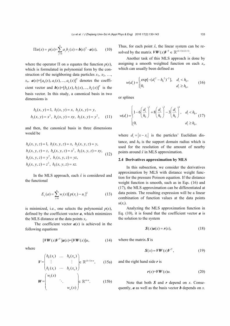
The numerical results with experimental tests of dam break at different time points within 1.0 s are shown in Fig. 3. As soon as the baffle holding the water at rest is removed, the fluid column confined between the two vertical walls begins to collapse under the action of gravity at t=0 s. When t=0.2 s, the collapsing water runs on the bottom wall and goes on to flow forward. At t=0.4 s, the rising water generates splashing drops after hitting the front wall, along with decreasing momentum. Until about t= 0.6 s, the water continues to fall due to the presence of the gravitational field. At t=0.8 s, the rising water column is dragged back, which hits the bottom again and begins to move back to the left. It can be ob-served that the numerical results of capturing water movement are in good agreement with the test phe-nomenon, proving that FPM has the ability to simu-late flow problems associated with complex defor-mation of free surface.

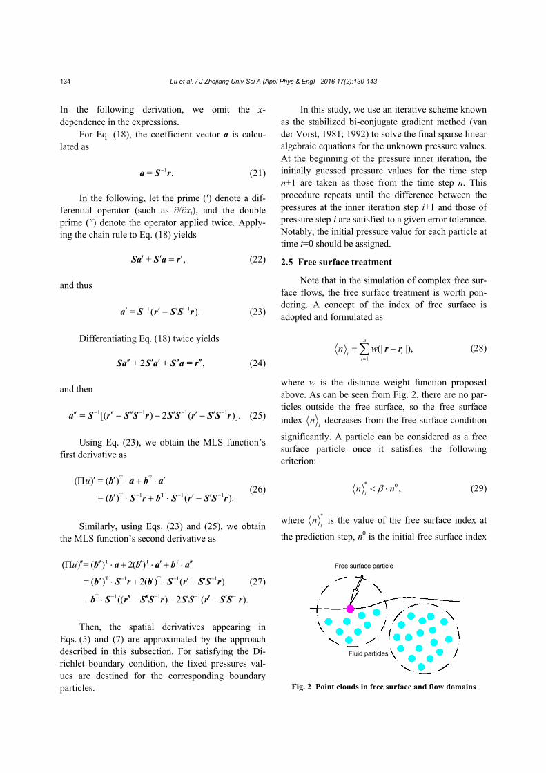
Figs. 4 and 5 present the velocity fields and pressure fields, respectively, at different time points. It can be seen that the fluid particles near the free Fig. 3 Numerical and experimental results of 2D dam break at different time points (t=0.0–0.8 s, Δt=0.2 s)


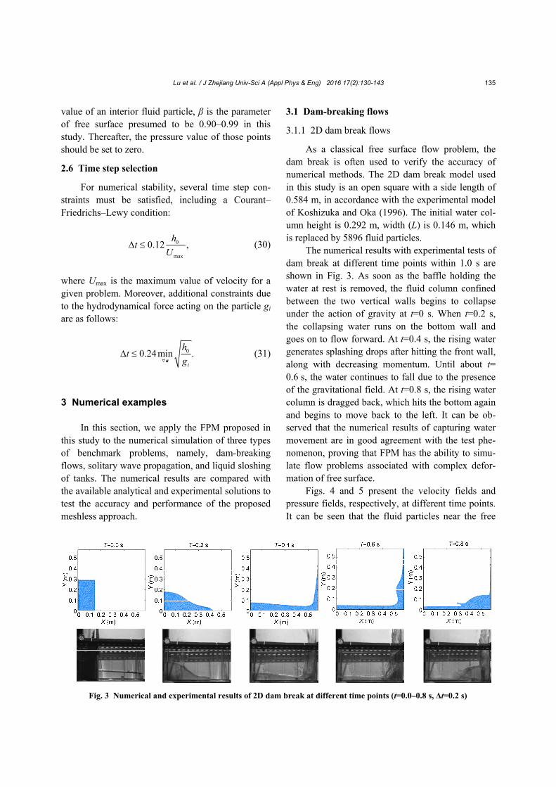
surface have greater velocities, which decrease with the distance at the initial stages of dam-breaking flow. Under the condition of high gradient velocity, the pressure fields’ distribution changes dramatically. As the fluid flows, the gradient of velocity gradually reduces so that the hydrostatic pressure distribution changes to be in a dominant role. Meanwhile, at t=0.4 and 0.8 s, the particles’ pressure near the cor-ner of the right wall is relatively high due to the high impact of water on the wall and the bottom.

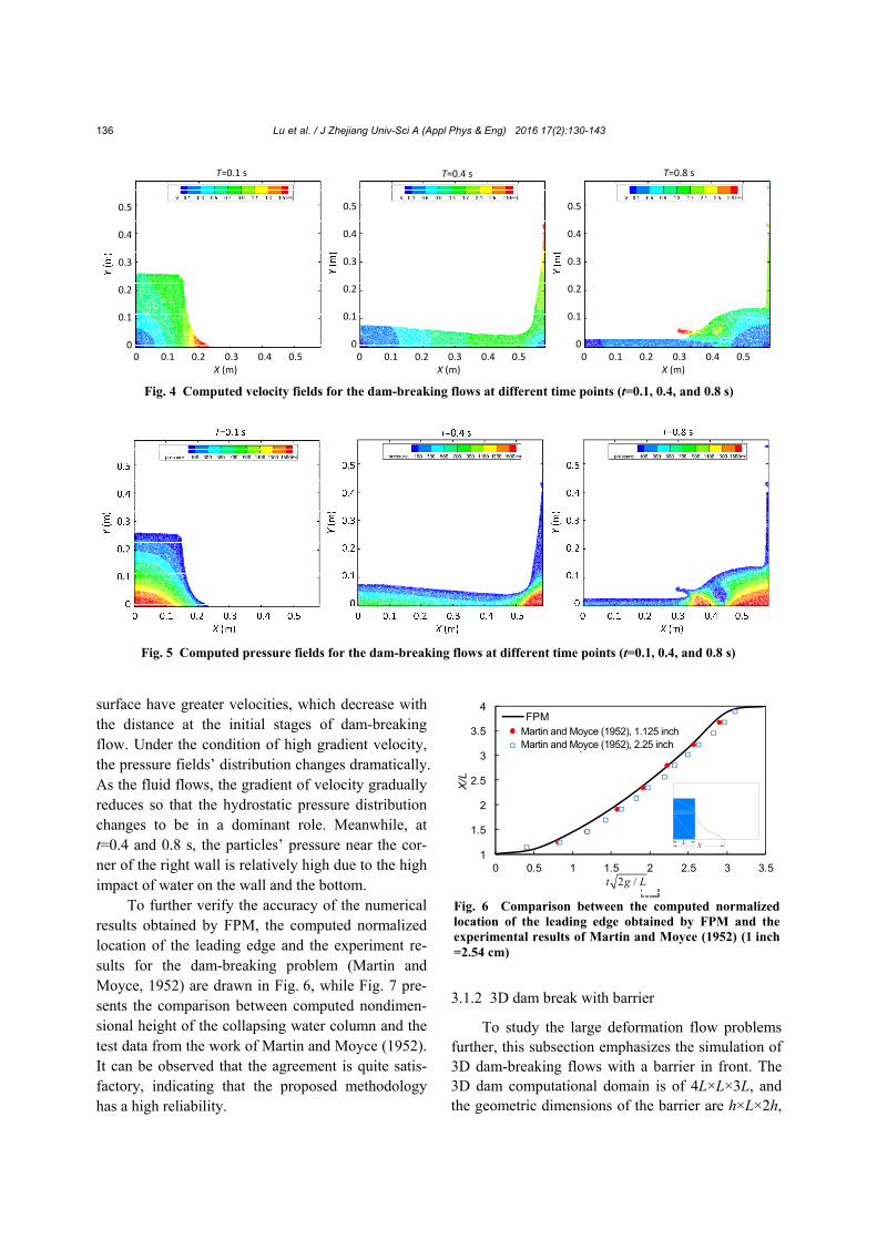
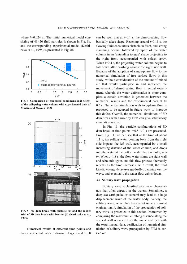
To further verify the accuracy of the numerical results obtained by FPM, the computed normalized location of the leading edge and the experiment re-sults for the dam-breaking problem (Martin and Moyce, 1952) are drawn in Fig. 6, while Fig. 7 pre-sents the comparison between computed nondimen-sional height of the collapsing water column and the test data from the work of Martin and Moyce (1952). It can be observed that the agreement is quite satis-factory, indicating that the proposed methodology has a high reliability.

3.1.2 3D dam break with barrier

To study the large deformation flow problems further, this subsection emphasizes the simulation of 3D dam-breaking flows with a barrier in front. The 3D dam computational domain is of 4L×L×3L, and the geometric dimensions of the barrier are h×L×2h,

Fig. 5 Computed pressure fields for the dam-breaking flows at different time points (t=0.1, 0.4, and 0.8 s)

0 0.1 0.2 0.3 0.4 0.5X (m)

0.5

0.4

0.3

0.2

0.1

0

0.5

0.4

0.3

0.2

0.1

0

0.5

0.4

0.3

0.2

0.1

00 0.1 0.2 0.3 0.4 0.5

X (m)0 0.1 0.2 0.3 0.4 0.5

X (m)

T=0.1 s T=0.4 s T=0.8 s

Fig. 4 Computed velocity fields for the dam-breaking flows at different time points (t=0.1, 0.4, and 0.8 s)

Fig. 6 Comparison between the computed normalized location of the leading edge obtained by FPM and the experimental results of Martin and Moyce (1952) (1 inch=2.54 cm)

1

1.5

2

2.5

3

3.5

4

0 0.5 1 1.5 2 2.5 3 3.5

X/L

FPMMartin&Moyce,1.125 inMartin&Moyce,2.25 in

2 /t g L

L X

Martin and Moyce (1952), 1.125 inch Martin and Moyce (1952), 2.25 inch


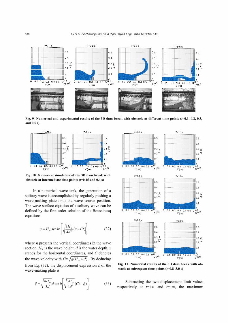
where h=0.024 m. The initial numerical model con-sisting of 41 420 fluid particles is shown in Fig. 8a, and the corresponding experimental model (Koshi-zuka et al., 1995) is presented in Fig. 8b.

Numerical results at different time points and

the experimental data are shown in Figs. 9 and 10. It

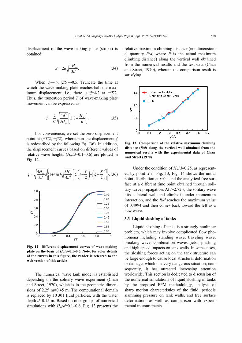
can be seen that at t=0.1 s, the dam-breaking flow basically takes shape. Reaching around t=0.15 s, the flowing fluid encounters obstacle in front, and strong slamming occurs, followed by uplift of the water column in an ‘extending tongue’ shape projecting to the right front, accompanied with splash spray. When t=0.4 s, the projecting water column begins to fall down after crashing against the right side wall. Because of the adoption of single-phase flow to the numerical simulation of free surface flows in this study, without consideration of the amount of mixed air that would participate in and influence the movement of dam-breaking flow in actual experi-ment, wherein the water deformation is more com-plex, a certain deviation is generated between the numerical results and the experimental data at t= 0.5 s. Numerical simulation with two-phase flow is proposed to be adopted in future work to improve this defect. Overall, the numerical simulation of 3D dam break with barrier by FPM can give satisfactory simulation results.

In Fig. 11, the particle configurations of 3D dam break at time points t=0.8–3.0 s are presented. From Fig. 11, we can see that at the time of about 1.1 s, the rolling water coming back from the right side impacts the left wall, accompanied by a small increasing distance of the water column, and drops into the water at the bottom under the force of gravi-ty. When t=1.8 s, the flow water slams the right wall and rebounds again, and this flow process alternately repeats as the time increases. As a result, the fluid kinetic energy decreases gradually, damping out the wave, and eventually the water flow calms down.

3.2 Solitary wave propagation

Solitary wave is classified as a wave phenome-non that often appears in the waters. Sometimes, a deep-sea earthquake or tsunami may lead to a huge displacement wave of the water body, namely, the solitary wave, which has been a hot issue in coastal engineering. A simulation of the propagation of soli-tary wave is presented in this section. Moreover, by comparing the maximum climbing distance along the vertical wall obtained from the numerical tests with the experimental data, verification of numerical sim-ulation of solitary wave propagation by FPM is car-ried out.

Fig. 8 3D dam break with obstacle (a) and the model trial of 3D dam break with barrier (b) (Koshizuka et al.,1995)

Z (

m)

(a)

(b)

0.2

0.4

0.6

0.8

1

0 0.5 1 1.5 2 2.5 3 3.5

H/2

L

FPM

Martin&Moyce,2.25 in

L

H

2 /t g L

Martin and Moyce (1952), 2.25 inch

H/(

2L)

Fig. 7 Comparison of computed nondimensional height of the collapsing water column with experimental data of Martin and Moyce (1952)


In a numerical wave tank, the generation of a solitary wave is accomplished by regularly pushing a wave-making plate onto the wave source position. The wave surface equation of a solitary wave can be defined by the first-order solution of the Boussinesq equation:

2 ww 3

3sec ( ) ,

4

HH h x Ct

d

(32)

where η presents the vertical coordinates in the wave section, Hw is the wave height, d is the water depth, x stands for the horizontal coordinates, and C denotes

the wave velocity with C= w( )g H d . By deducing

from Eq. (32), the displacement expression ξ of the wave-making plate is

w w3

4 3tan ( ) .

3 4

H Hd h Ct

d d

(33)

Subtracting the two displacement limit values

respectively at t=+∞ and t=−∞, the maximum

Fig. 9 Numerical and experimental results of the 3D dam break with obstacle at different time points (t=0.1, 0.2, 0.3,and 0.5 s)

Fig. 10 Numerical simulation of the 3D dam break with obstacle at intermediate time points (t=0.15 and 0.4 s)

Z(m

)

Z(m

)

Fig. 11 Numerical results of the 3D dam break with ob-stacle at subsequent time points (t=0.8–3.0 s)

0 0.1 0.2 0.3 0.4 0.5 0Y (m)

0.5

0.4

0.3

0.2

0.1

0

T=1.1 s

-0.1

X (m)0 0.1 0.2 0.3 0.4 0.5 0

Y (m)

0.5

0.4

0.3

0.2

0.1

0

T=0.8 s

-0.1

X (m)

0 0.1 0.2 0.3 0.4 0.5 0Y (m)

0.5

0.4

0.3

0.2

0.1

0

T=1.8 s

-0.1

X (m)0 0.1 0.2 0.3 0.4 0.5 0

Y (m)

0.5

0.4

0.3

0.2

0.1

0

T=1.4 s

-0.1

X (m)

0 0.1 0.2 0.3 0.4 0.5 0Y (m)

0.5

0.4

0.3

0.2

0.1

0

T=3.0 s

-0.1

X (m)0 0.1 0.2 0.3 0.4 0.5 0

Y (m)

0.5

0.4

0.3

0.2

0.1

0

T=2.2 s

-0.1

X (m)


displacement of the wave-making plate (stroke) is obtained:

w42 .

3

HS d

d (34)

When |t|→∞, |ξ/S|→0.5. Truncate the time at

which the wave-making plate reaches half the max-imum displacement, i.e., there is ξ=S/2 at t=T/2. Thus, the truncation period T of wave-making plate movement can be expressed as

3

w

w

2 43.8 .

3

HdT

C H d

(35)

For convenience, we set the zero displacement

point at (−T/2, −ξ/2), whereupon the displacement ξ is redescribed by the following Eq. (36). In addition, the displacement curves based on different values of relative wave heights (Hw/d=0.1–0.6) are plotted in Fig. 12.

w w3

4 31 tan .

3 2 24

H H T Sd h C t

d d

(36)

The numerical wave tank model is established

depending on the solitary wave experiment (Chan and Street, 1970), which is in the geometric dimen-sions of 2.25 m×0.45 m. The computational domain is replaced by 10 301 fluid particles, with the water depth d=0.15 m. Based on nine groups of numerical simulations with Hw/d=0.1–0.6, Fig. 13 presents the

relative maximum climbing distance (nondimension-al quantity R/d, where R is the actual maximum climbing distance) along the vertical wall obtained from the numerical results and the test data (Chan and Street, 1970), wherein the comparison result is satisfying.

Under the condition of Hw/d=0.25, as represent-

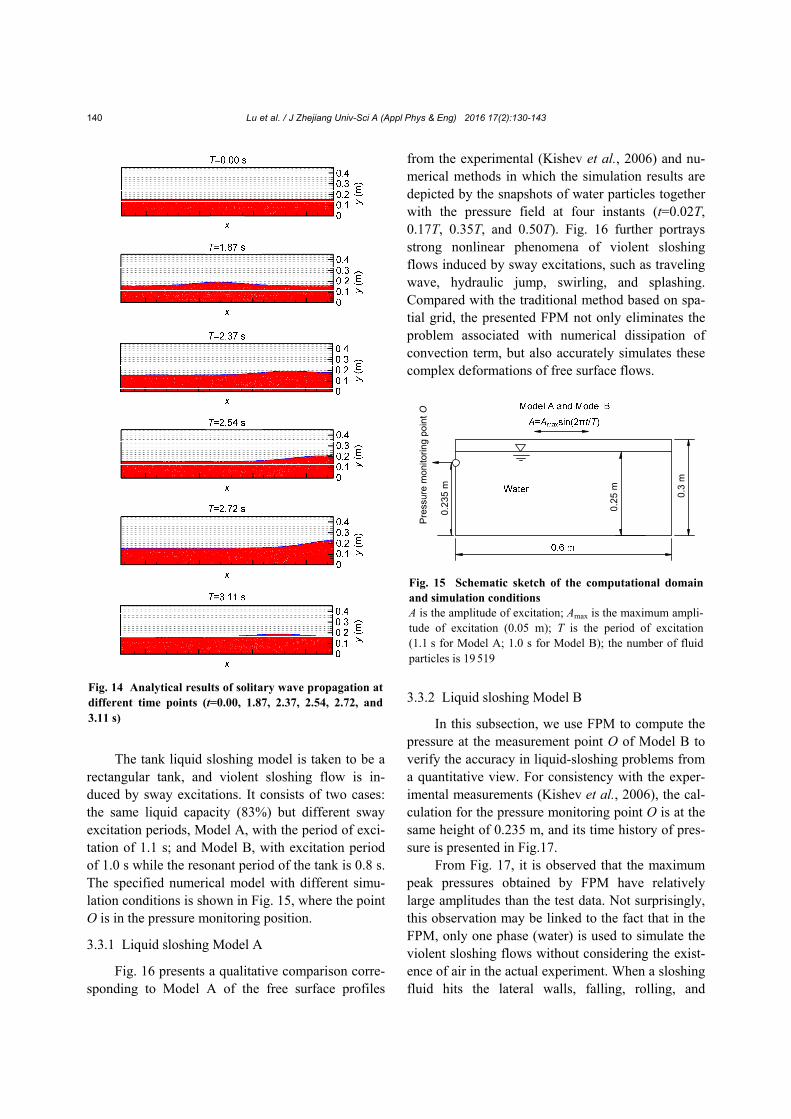
ed by point X in Fig. 13, Fig. 14 shows the initial point distribution at t=0 s and the analytical free sur-face at a different time point obtained through soli-tary wave propagation. At t=2.72 s, the solitary wave hits a lateral wall and climbs it under momentum interaction, and the R/d reaches the maximum value of 0.4994 and then comes back toward the left as a new wave.

3.3 Liquid sloshing of tanks

Liquid sloshing of tanks is a strongly nonlinear problem, which may involve complicated flow phe-nomena including standing wave, traveling wave, breaking wave, combination waves, jets, splashing and high-speed impacts on tank walls. In some cases, the sloshing forces acting on the tank structure can be large enough to cause local structural deformation or damage, which is a very dangerous situation; con-sequently, it has attracted increasing attention worldwide. This section is dedicated to discussion of the numerical simulations of liquid sloshing in tanks by the proposed FPM methodology, analysis of sharp motion characteristics of the fluid, periodic slamming pressure on tank walls, and free surface deformation, as well as comparison with experi-mental measurements.

Fig. 13 Comparison of the relative maximum climbing distance (R/d) along the vertical wall obtained from the numerical results with the experimental data of Chan and Street (1970)

Fig. 12 Different displacement curves of wave-makingplate on the basis of Hw/d=0.1–0.6. Note: for color details of the curves in this figure, the reader is referred to the web version of this article

0

0.2

0.4

0.6

0.8

1.0

0 0.2 0.4 0.6 0.8 1t/T

0.10

0.20

0.25

0.30

0.36

0.45

0.50

0.55

0.60


The tank liquid sloshing model is taken to be a

rectangular tank, and violent sloshing flow is in-duced by sway excitations. It consists of two cases: the same liquid capacity (83%) but different sway excitation periods, Model A, with the period of exci-tation of 1.1 s; and Model B, with excitation period of 1.0 s while the resonant period of the tank is 0.8 s. The specified numerical model with different simu-lation conditions is shown in Fig. 15, where the point O is in the pressure monitoring position.

3.3.1 Liquid sloshing Model A

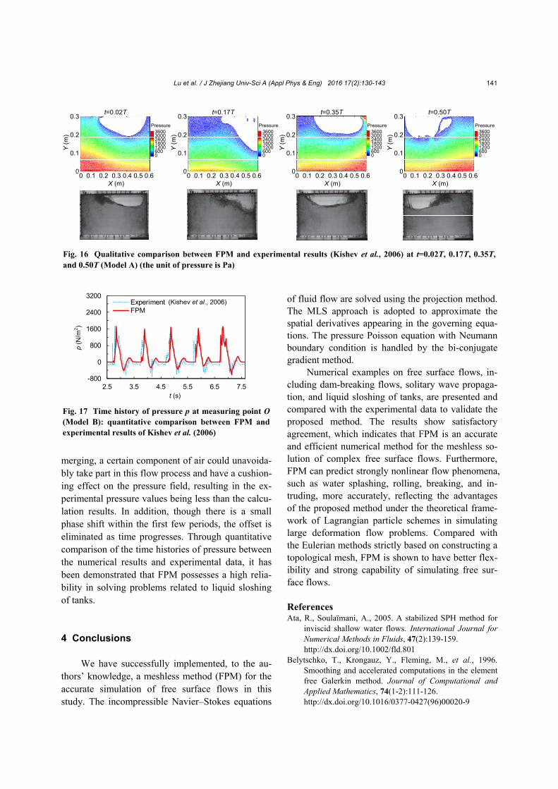
Fig. 16 presents a qualitative comparison corre-sponding to Model A of the free surface profiles

from the experimental (Kishev et al., 2006) and nu-merical methods in which the simulation results are depicted by the snapshots of water particles together with the pressure field at four instants (t=0.02T, 0.17T, 0.35T, and 0.50T). Fig. 16 further portrays strong nonlinear phenomena of violent sloshing flows induced by sway excitations, such as traveling wave, hydraulic jump, swirling, and splashing. Compared with the traditional method based on spa-tial grid, the presented FPM not only eliminates the problem associated with numerical dissipation of convection term, but also accurately simulates these complex deformations of free surface flows.

3.3.2 Liquid sloshing Model B

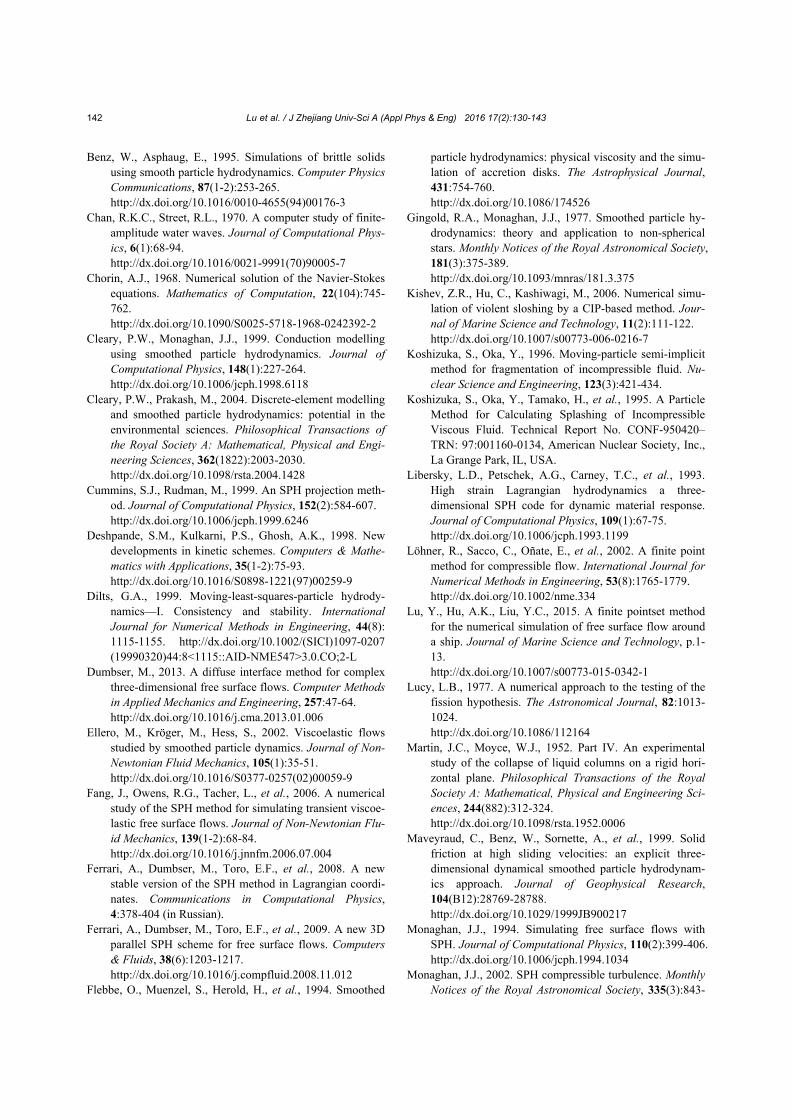
In this subsection, we use FPM to compute the pressure at the measurement point O of Model B to verify the accuracy in liquid-sloshing problems from a quantitative view. For consistency with the exper-imental measurements (Kishev et al., 2006), the cal-culation for the pressure monitoring point O is at the same height of 0.235 m, and its time history of pres-sure is presented in Fig.17.

From Fig. 17, it is observed that the maximum peak pressures obtained by FPM have relatively large amplitudes than the test data. Not surprisingly, this observation may be linked to the fact that in the FPM, only one phase (water) is used to simulate the violent sloshing flows without considering the exist-ence of air in the actual experiment. When a sloshing fluid hits the lateral walls, falling, rolling, and

Fig. 15 Schematic sketch of the computational domain and simulation conditions A is the amplitude of excitation; Amax is the maximum ampli-tude of excitation (0.05 m); T is the period of excitation(1.1 s for Model A; 1.0 s for Model B); the number of fluid particles is 19 519

0.3

m

0.25

m

0.23

5m

Pre

ssur

e m

onito

ring

poi

nt O

Fig. 14 Analytical results of solitary wave propagation at different time points (t=0.00, 1.87, 2.37, 2.54, 2.72, and 3.11 s)


merging, a certain component of air could unavoida-bly take part in this flow process and have a cushion-ing effect on the pressure field, resulting in the ex-perimental pressure values being less than the calcu-lation results. In addition, though there is a small phase shift within the first few periods, the offset is eliminated as time progresses. Through quantitative comparison of the time histories of pressure between the numerical results and experimental data, it has been demonstrated that FPM possesses a high relia-bility in solving problems related to liquid sloshing of tanks.

4 Conclusions We have successfully implemented, to the au-

thors’ knowledge, a meshless method (FPM) for the accurate simulation of free surface flows in this study. The incompressible Navier–Stokes equations

of fluid flow are solved using the projection method. The MLS approach is adopted to approximate the spatial derivatives appearing in the governing equa-tions. The pressure Poisson equation with Neumann boundary condition is handled by the bi-conjugate gradient method.

Numerical examples on free surface flows, in-cluding dam-breaking flows, solitary wave propaga-tion, and liquid sloshing of tanks, are presented and compared with the experimental data to validate the proposed method. The results show satisfactory agreement, which indicates that FPM is an accurate and efficient numerical method for the meshless so-lution of complex free surface flows. Furthermore, FPM can predict strongly nonlinear flow phenomena, such as water splashing, rolling, breaking, and in-truding, more accurately, reflecting the advantages of the proposed method under the theoretical frame-work of Lagrangian particle schemes in simulating large deformation flow problems. Compared with the Eulerian methods strictly based on constructing a topological mesh, FPM is shown to have better flex-ibility and strong capability of simulating free sur-face flows.

References Ata, R., Soulaïmani, A., 2005. A stabilized SPH method for

inviscid shallow water flows. International Journal for Numerical Methods in Fluids, 47(2):139-159. http://dx.doi.org/10.1002/fld.801

Belytschko, T., Krongauz, Y., Fleming, M., et al., 1996. Smoothing and accelerated computations in the element free Galerkin method. Journal of Computational and Applied Mathematics, 74(1-2):111-126. http://dx.doi.org/10.1016/0377-0427(96)00020-9

Fig. 16 Qualitative comparison between FPM and experimental results (Kishev et al., 2006) at t=0.02T, 0.17T, 0.35T, and 0.50T (Model A) (the unit of pressure is Pa)

0.3

0.2

0.1

00 0.1 0.2 0.3 0.4 0.5 0.6

X (m)

t=0.02T

360030002400180012006000

Pressure

Y(m

)

0.3

0.2

0.1

00 0.1 0.2 0.3 0.4 0.5 0.6

X (m)

t=0.17T

360030002400180012006000

Pressure

Y(m

)

0.3

0.2

0.1

00 0.1 0.2 0.3 0.4 0.5 0.6

X (m)

t=0.35T

360030002400180012006000

Pressure

Y(m

)

0.3

0.2

0.1

00 0.1 0.2 0.3 0.4 0.5 0.6

X (m)

t=0.50T

360030002400180012006000

Pressure

Y(m

)

Fig. 17 Time history of pressure p at measuring point O(Model B): quantitative comparison between FPM and experimental results of Kishev et al. (2006)

-800

0

800

1600

2400

3200

2.5 3.5 4.5 5.5 6.5 7.5

p/(

N/m

2 )

t /s

Experiment (Zdravko et al., 2006)FPM

(Kishev et al., 2006)

p (N

/m2)

t (s)


Benz, W., Asphaug, E., 1995. Simulations of brittle solids using smooth particle hydrodynamics. Computer Physics Communications, 87(1-2):253-265. http://dx.doi.org/10.1016/0010-4655(94)00176-3

Chan, R.K.C., Street, R.L., 1970. A computer study of finite-amplitude water waves. Journal of Computational Phys-ics, 6(1):68-94. http://dx.doi.org/10.1016/0021-9991(70)90005-7

Chorin, A.J., 1968. Numerical solution of the Navier-Stokes equations. Mathematics of Computation, 22(104):745-762. http://dx.doi.org/10.1090/S0025-5718-1968-0242392-2

Cleary, P.W., Monaghan, J.J., 1999. Conduction modelling using smoothed particle hydrodynamics. Journal of Computational Physics, 148(1):227-264. http://dx.doi.org/10.1006/jcph.1998.6118

Cleary, P.W., Prakash, M., 2004. Discrete-element modelling and smoothed particle hydrodynamics: potential in the environmental sciences. Philosophical Transactions of the Royal Society A: Mathematical, Physical and Engi-neering Sciences, 362(1822):2003-2030. http://dx.doi.org/10.1098/rsta.2004.1428

Cummins, S.J., Rudman, M., 1999. An SPH projection meth-od. Journal of Computational Physics, 152(2):584-607. http://dx.doi.org/10.1006/jcph.1999.6246

Deshpande, S.M., Kulkarni, P.S., Ghosh, A.K., 1998. New developments in kinetic schemes. Computers & Mathe-matics with Applications, 35(1-2):75-93. http://dx.doi.org/10.1016/S0898-1221(97)00259-9

Dilts, G.A., 1999. Moving-least-squares-particle hydrody-namics—I. Consistency and stability. International Journal for Numerical Methods in Engineering, 44(8): 1115-1155. http://dx.doi.org/10.1002/(SICI)1097-0207 (19990320)44:8<1115::AID-NME547>3.0.CO;2-L

Dumbser, M., 2013. A diffuse interface method for complex three-dimensional free surface flows. Computer Methods in Applied Mechanics and Engineering, 257:47-64. http://dx.doi.org/10.1016/j.cma.2013.01.006

Ellero, M., Kröger, M., Hess, S., 2002. Viscoelastic flows studied by smoothed particle dynamics. Journal of Non-Newtonian Fluid Mechanics, 105(1):35-51. http://dx.doi.org/10.1016/S0377-0257(02)00059-9

Fang, J., Owens, R.G., Tacher, L., et al., 2006. A numerical study of the SPH method for simulating transient viscoe-lastic free surface flows. Journal of Non-Newtonian Flu-id Mechanics, 139(1-2):68-84. http://dx.doi.org/10.1016/j.jnnfm.2006.07.004

Ferrari, A., Dumbser, M., Toro, E.F., et al., 2008. A new stable version of the SPH method in Lagrangian coordi-nates. Communications in Computational Physics, 4:378-404 (in Russian).

Ferrari, A., Dumbser, M., Toro, E.F., et al., 2009. A new 3D parallel SPH scheme for free surface flows. Computers & Fluids, 38(6):1203-1217. http://dx.doi.org/10.1016/j.compfluid.2008.11.012

Flebbe, O., Muenzel, S., Herold, H., et al., 1994. Smoothed

particle hydrodynamics: physical viscosity and the simu-lation of accretion disks. The Astrophysical Journal, 431:754-760. http://dx.doi.org/10.1086/174526

Gingold, R.A., Monaghan, J.J., 1977. Smoothed particle hy-drodynamics: theory and application to non-spherical stars. Monthly Notices of the Royal Astronomical Society, 181(3):375-389. http://dx.doi.org/10.1093/mnras/181.3.375

Kishev, Z.R., Hu, C., Kashiwagi, M., 2006. Numerical simu-lation of violent sloshing by a CIP-based method. Jour-nal of Marine Science and Technology, 11(2):111-122. http://dx.doi.org/10.1007/s00773-006-0216-7

Koshizuka, S., Oka, Y., 1996. Moving-particle semi-implicit method for fragmentation of incompressible fluid. Nu-clear Science and Engineering, 123(3):421-434.

Koshizuka, S., Oka, Y., Tamako, H., et al., 1995. A Particle Method for Calculating Splashing of Incompressible Viscous Fluid. Technical Report No. CONF-950420– TRN: 97:001160-0134, American Nuclear Society, Inc., La Grange Park, IL, USA.

Libersky, L.D., Petschek, A.G., Carney, T.C., et al., 1993. High strain Lagrangian hydrodynamics a three-dimensional SPH code for dynamic material response. Journal of Computational Physics, 109(1):67-75. http://dx.doi.org/10.1006/jcph.1993.1199

Löhner, R., Sacco, C., Oñate, E., et al., 2002. A finite point method for compressible flow. International Journal for Numerical Methods in Engineering, 53(8):1765-1779. http://dx.doi.org/10.1002/nme.334

Lu, Y., Hu, A.K., Liu, Y.C., 2015. A finite pointset method for the numerical simulation of free surface flow around a ship. Journal of Marine Science and Technology, p.1-13. http://dx.doi.org/10.1007/s00773-015-0342-1

Lucy, L.B., 1977. A numerical approach to the testing of the fission hypothesis. The Astronomical Journal, 82:1013-1024. http://dx.doi.org/10.1086/112164

Martin, J.C., Moyce, W.J., 1952. Part IV. An experimental study of the collapse of liquid columns on a rigid hori-zontal plane. Philosophical Transactions of the Royal Society A: Mathematical, Physical and Engineering Sci-ences, 244(882):312-324. http://dx.doi.org/10.1098/rsta.1952.0006

Maveyraud, C., Benz, W., Sornette, A., et al., 1999. Solid friction at high sliding velocities: an explicit three-dimensional dynamical smoothed particle hydrodynam-ics approach. Journal of Geophysical Research, 104(B12):28769-28788. http://dx.doi.org/10.1029/1999JB900217

Monaghan, J.J., 1994. Simulating free surface flows with SPH. Journal of Computational Physics, 110(2):399-406. http://dx.doi.org/10.1006/jcph.1994.1034

Monaghan, J.J., 2002. SPH compressible turbulence. Monthly Notices of the Royal Astronomical Society, 335(3):843-


852. http://dx.doi.org/10.1046/j.1365-8711.2002.05678.x

Monaghan, J.J., Kocharyan, A., 1995. SPH simulation of multi-phase flow. Computer Physics Communications, 87(1-2):225-235. http://dx.doi.org/10.1016/0010-4655(94)00174-Z

Morris, J.P., 2000. Simulating surface tension with smoothed particle hydrodynamics. International Journal for Nu-merical Methods in Fluids, 33(3):333-353. http://dx.doi.org/10.1002/1097-0363(20000615)33:3<33 3::AID-FLD11>3.0.CO;2-7

Morris, J.P., Fox, P.J., Zhu, Y., 1997. Modeling low Reyn-olds number incompressible flows using SPH. Journal of Computational Physics, 136(1):214-226. http://dx.doi.org/10.1006/jcph.1997.5776

Oger, L., Savage, S.B., 1999. Smoothed particle hydrody-namics for cohesive grains. Computer Methods in Ap-plied Mechanics and Engineering, 180(1-2):169-183. http://dx.doi.org/10.1016/S0045-7825(99)00054-7

Oñate, E., Idelsohn, S.R., 1998. A mesh-free finite point method for advective-diffusive transport and fluid flow problems. Computational Mechanics, 21(4-5):283-292. http://dx.doi.org/10.1007/s004660050304

Oñate, E., Idelsohn, S.R., Zienkievicz, O.C., et al., 1996a. A finite point method in computational mechanics to con-vective transport and fluid flow. International Journal for Numerical Methods in Engineering, 39(22):3839-3866. http://dx.doi.org/10.1002/(SICI)1097-0207(19961130)39: 22<3839::AID-NME27>3.0.CO;2-R

Oñate, E., Idelsohn, S.R., Zienkievicz, O.C., et al., 1996b. A stabilized finite point method for analysis of fluid me-chanics problems. Computer Methods in Applied Me-chanics and Engineering, 139(1-4):315-346. http://dx.doi.org/10.1016/S0045-7825(96)01088-2

Oñate, E., Sacco, C., Idelsohn, S.R., 2000. A finite point method for incompressible flow problems. Computing and Visualization in Science, 3(1-2):67-75. http://dx.doi.org/10.1007/s007910050053

Shao, S., Lo, E.Y., 2003. Incompressible SPH method for simulating Newtonian and non-Newtonian flows with a free surface. Advances in Water Resources, 26(7):787-800. http://dx.doi.org/10.1016/S0309-1708(03)00030-7

Song, C., Zhang, H.X., Huang, J., et al., 2006. Meshless sim-ulation for skeleton driven elastic deformation. Journal of Zhejiang University-SCIENCE A, 7(9):1596-1602. http://dx.doi.org/10.1631/jzus.2006.A1596

Takeda, H., Miyama, S.M., Sekiya, M., 1994. Numerical simulation of viscous flow by smoothed particle hydro-dynamics. Progress of Theoretical Physics, 92(5):939-960.

http://dx.doi.org/10.1143/ptp/92.5.939 van der Vorst, H.A., 1981. Iterative solution methods for

certain sparse linear systems with a non-symmetric ma-trix arising from PDE-problems. Journal of Computa-tional Physics, 44(1):1-19. http://dx.doi.org/10.1016/0021-9991(81)90034-6

van der Vorst, H.A., 1992. Bi-CGSTAB: a fast and smoothly converging variant of Bi-CG for the solution of non-symmetric linear systems. SIAM Journal on Scientific and Statistical Computing, 13(2):631-644. http://dx.doi.org/10.1137/0913035

Watkins, S.J., Bhattal, A.S., Francis, N., et al., 1996. A new prescription for viscosity in smoothed particle hydrody-namics. Astronomy and Astrophysics Supplement Series, 119(1):177-187. http://dx.doi.org/10.1051/aas:1996104

中文概要

题目：一种基于移动最小二乘无网格法的自由面流动

数值研究

目的：自由面流动中的大变形、复杂几何边界等问题

一直备受工程界的关注。本文基于拉格朗日观

点，采用移动最小二乘的无网格技术数值模拟

流场，研究溃坝流、孤立波传播及液舱晃荡等

复杂变形的自由面流动，验证该方法的准确性

与可靠性。

创新点：1. 通过不可压缩 Navier–Stokes 方程，采用投影

法推导出压力与速度之间的关系；2. 借助移动

最小二乘法的思想，对压力泊松方程进行离散

求解。

方法：1. 通过理论推导，得出不可压缩流动中压力与

速度之间的泊松方程式，并采用移动最小二乘

法离散求解该偏微分方程；2. 采用数值计算，

对自由面流动问题中的三个典型算例进行模

拟；3. 将数值计算结果与文献中的试验结果进

行比较。

结论：1. 基于移动最小二乘的无网格法能够较准确地

模拟自由面流动中的液体迸溅、翻滚、破碎以

及入水等强非线性现象，在处理大变形流动问

题时体现出较好的灵活性及较强的自由面模拟

能力；2. 对比分析数值计算结果与试验现象，

得到一致性较好的结果，验证了该无网格法的

准确性与可靠性。

关键词：无网格法；移动最小二乘；自由面流动；有限

点法；溃坝流；孤立波传播；液舱晃荡

Documents

A meshless method based on moving least squares … · A meshless method based on moving least squares for the simulation of free ... HAN1 (1College of Shipbuilding Engineering,