A Linear Non-Gaussian Acyclic Model for Causal …A Linear Non-Gaussian Acyclic Model for Causal Discovery Shohei Shimizu∗ [email protected] JP Patrik O. Hoyer PATRIK.HOYER@HELSINKI

Journal of Machine Learning Research 7 (2006) 2003-2030 Submitted 3/06; Revised 7/06; Published 10/06

A Linear Non-Gaussian Acyclic Model for Causal Discovery

Shohei Shimizu∗ [email protected]

Patrik O. Hoyer [email protected]

Aapo Hyvarinen [email protected]

Antti Kerminen [email protected]

Helsinki Institute for Information Technology, Basic Research UnitDepartment of Computer ScienceUniversity of HelsinkiFIN-00014, Finland

Editor: Michael Jordan

AbstractIn recent years, several methods have been proposed for the discovery of causal structure fromnon-experimental data. Such methods make various assumptions on the data generating processto facilitate its identification from purely observational data. Continuing this line of research, weshow how to discover the complete causal structure of continuous-valued data, under the assump-tions that (a) the data generating process is linear, (b) there are no unobserved confounders, and (c)disturbance variables have non-Gaussian distributions of non-zero variances. The solution relies onthe use of the statistical method known as independent component analysis, and does not requireany pre-specified time-ordering of the variables. We provide a complete Matlab package for per-forming this LiNGAM analysis (short for Linear Non-Gaussian Acyclic Model), and demonstratethe effectiveness of the method using artificially generated data and real-world data.

Keywords: independent component analysis, non-Gaussianity, causal discovery, directed acyclicgraph, non-experimental data

1. Introduction

Several authors (Spirtes et al., 2000; Pearl, 2000) have recently formalized concepts related tocausality using probability distributions defined on directed acyclic graphs. This line of researchemphasizes the importance of understanding the process which generated the data, rather than onlycharacterizing the joint distribution of the observed variables. The reasoning is that a causal un-derstanding of the data is essential to be able to predict the consequences of interventions, such assetting a given variable to some specified value.

One of the main questions one can answer using this kind of theoretical framework is: ‘Underwhat circumstances and in what way can one determine causal structure on the basis of observationaldata alone?’. In many cases it is impossible or too expensive to perform controlled experiments,and hence methods for discovering likely causal relations from uncontrolled data would be veryvaluable.

Existing discovery algorithms (Spirtes et al., 2000; Pearl, 2000) generally work in one of twosettings. In the case of discrete data, no functional form for the dependencies is usually assumed.

∗. Current address: The Institute of Statistical Mathematics, 4-6-7 Minami-Azabu, Minato-ku, Tokyo 106-8569, Japan

c©2006 Shimizu, Hoyer, Hyvarinen and Kerminen.

SHIMIZU, HOYER, HYVARINEN AND KERMINEN

x3

4 -3

2

x2

e2

e1e1 e3e2

e3

x1

x3

0.2 1

-5-2

x4

x2

e4

x1 e4

e2e3 x3

2

-5 3

x1

x2

e1

x4 e2

0.5

x1

e1

x2 e1

0.5

x2

e2

x1

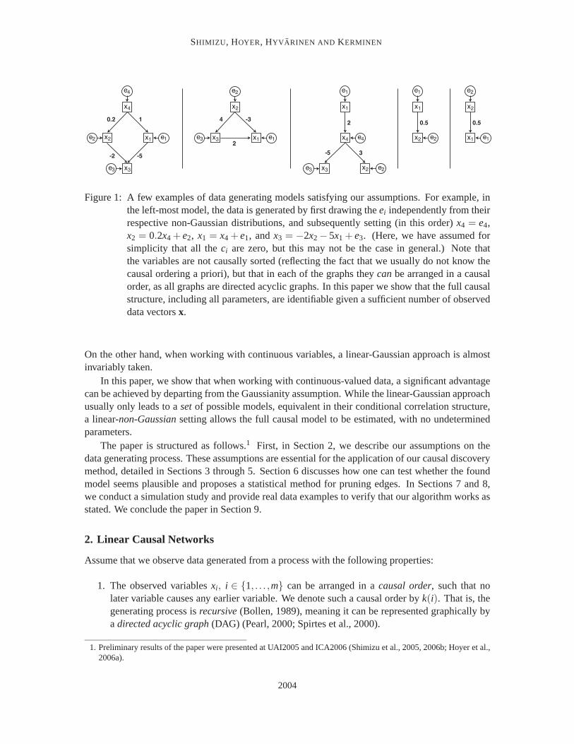
Figure 1: A few examples of data generating models satisfying our assumptions. For example, inthe left-most model, the data is generated by first drawing the ei independently from theirrespective non-Gaussian distributions, and subsequently setting (in this order) x4 = e4,x2 = 0.2x4 + e2, x1 = x4 + e1, and x3 = −2x2 − 5x1 + e3. (Here, we have assumed forsimplicity that all the ci are zero, but this may not be the case in general.) Note thatthe variables are not causally sorted (reflecting the fact that we usually do not know thecausal ordering a priori), but that in each of the graphs they can be arranged in a causalorder, as all graphs are directed acyclic graphs. In this paper we show that the full causalstructure, including all parameters, are identifiable given a sufficient number of observeddata vectors x.

On the other hand, when working with continuous variables, a linear-Gaussian approach is almostinvariably taken.

In this paper, we show that when working with continuous-valued data, a significant advantagecan be achieved by departing from the Gaussianity assumption. While the linear-Gaussian approachusually only leads to a set of possible models, equivalent in their conditional correlation structure,a linear-non-Gaussian setting allows the full causal model to be estimated, with no undeterminedparameters.

The paper is structured as follows.1 First, in Section 2, we describe our assumptions on thedata generating process. These assumptions are essential for the application of our causal discoverymethod, detailed in Sections 3 through 5. Section 6 discusses how one can test whether the foundmodel seems plausible and proposes a statistical method for pruning edges. In Sections 7 and 8,we conduct a simulation study and provide real data examples to verify that our algorithm works asstated. We conclude the paper in Section 9.

2. Linear Causal Networks

Assume that we observe data generated from a process with the following properties:

1. The observed variables xi, i ∈ {1, . . . ,m} can be arranged in a causal order, such that nolater variable causes any earlier variable. We denote such a causal order by k(i). That is, thegenerating process is recursive (Bollen, 1989), meaning it can be represented graphically bya directed acyclic graph (DAG) (Pearl, 2000; Spirtes et al., 2000).

1. Preliminary results of the paper were presented at UAI2005 and ICA2006 (Shimizu et al., 2005, 2006b; Hoyer et al.,2006a).

2004

A LINEAR NON-GAUSSIAN ACYCLIC MODEL FOR CAUSAL DISCOVERY

2. The value assigned to each variable xi is a linear function of the values already assigned tothe earlier variables, plus a ‘disturbance’ (noise) term ei, and plus an optional constant termci, that is

xi = ∑k( j)<k(i)

bi jx j + ei + ci.

3. The disturbances ei are all continuous-valued random variables with non-Gaussian distribu-tions of non-zero variances, and the ei are independent of each other, that is, p(e1, . . . ,em) =∏i pi(ei).

A model with these three properties we call a Linear, Non-Gaussian, Acyclic Model, abbreviatedLiNGAM.

We assume that we are able to observe a large number of data vectors x (which contain the com-ponents xi), and each is generated according to the above-described process, with the same causalorder k(i), same coefficients bi j, same constants ci, and the disturbances ei sampled independentlyfrom the same distributions.

Note that the above assumptions imply that there are no unobserved confounders (Pearl, 2000).2

Spirtes et al. (2000) call this the causally sufficient case. Also note that we do not require ‘stability’in the sense as described by Pearl (2000), that is, ‘faithfulness’ (Spirtes et al., 2000) of the generatingmodel. See Figure 1 for a few examples of data models fulfilling the assumptions of our model.

A key difference to most earlier work on the linear, causally sufficient, case is the assumption ofnon-Gaussianity of the disturbances. In most work, an explicit or implicit assumption of Gaussianityhas been made (Bollen, 1989; Geiger and Heckerman, 1994; Spirtes et al., 2000). An assumption ofGaussianity of disturbance variables makes the full joint distribution over the xi Gaussian, and thecovariance matrix of the data embodies all one could possibly learn from observing the variables.Hence, all conditional correlations can be computed from the covariance matrix, and discoveryalgorithms based on conditional independence can be easily applied.

However, it turns out, as we will show below, that an assumption of non-Gaussianity may actu-ally be more useful. In particular, it turns out that when this assumption is valid, the complete causalstructure can in fact be estimated, without any prior information on a causal ordering of the vari-ables. This is in stark contrast to what can be done in the Gaussian case: algorithms based only onsecond-order statistics (i.e., the covariance matrix) are generally not able to discern the full causalstructure in most cases. The simplest such case is that of two variables, x1 and x2. A method basedonly on the covariance matrix has no way of preferring x1 → x2 over the reverse model x1 ← x2;indeed the two are indistinguishable in terms of the covariance matrix (Spirtes et al., 2000). How-ever, assuming non-Gaussianity, one can actually discover the direction of causality, as shown byDodge and Rousson (2001) and Shimizu and Kano (2006). This result can be extended to severalvariables (Shimizu et al., 2006a). Here, we further develop the method so as to estimate the fullmodel including all parameters, and we propose a number of tests to prune the graph and to seewhether the estimated model fits the data.

2. A simple explanation is as follows: Denote by f hidden common causes and by G its connection strength matrix.Then a new model with hidden common causes f can be written as x = Bx + G f + e′. Since common causesf introduce some dependency between e = G f + e′, the new model is different from the LiNGAM model withindependent (not merely uncorrelated) disturbances e. See Hoyer et al. (2006b) for details.

2005


3. Model Identification Using Independent Component Analysis

The key to the solution to the linear discovery problem is to realize that the observed variables arelinear functions of the disturbance variables, and the disturbance variables are mutually independentand non-Gaussian. If we as preprocessing subtract out the mean of each variable xi, we are left withthe following system of equations:

x = Bx+ e, (1)

where B is a matrix that could be permuted (by simultaneous equal row and column permutations)to strict lower triangularity if one knew a causal ordering k(i) of the variables (Bollen, 1989). (Strictlower triangularity is here defined as lower triangular with all zeros on the diagonal.) Solving for xone obtains

x = Ae, (2)

where A = (I−B)−1. Again, A could be permuted to lower triangularity (although not strict lowertriangularity, actually in this case all diagonal elements will be non-zero) with an appropriate per-mutation k(i). Taken together, Equation (2) and the independence and non-Gaussianity of the com-ponents of e define the standard linear independent component analysis model.

Independent component analysis (ICA) (Comon, 1994; Hyvarinen et al., 2001) is a fairly re-cent statistical technique for identifying a linear model such as that given in Equation (2). If theobserved data is a linear, invertible mixture of non-Gaussian independent components, it can beshown (Comon, 1994) that the mixing matrix A is identifiable (up to scaling and permutation ofthe columns, as discussed below) given enough observed data vectors x. Furthermore, efficientalgorithms for estimating the mixing matrix are available (Hyvarinen, 1999).

We again want to emphasize that ICA uses non-Gaussianity (that is, more than covariance in-formation) to estimate the mixing matrix A (or equivalently its inverse W = A−1). For Gaussiandisturbance variables ei, ICA cannot in general find the correct mixing matrix because many differ-ent mixing matrices yield the same covariance matrix, which in turn implies the exact same Gaussianjoint density (Hyvarinen et al., 2001). Our requirement for non-Gaussianity of disturbance variablesstems from the same requirement in ICA.

While ICA is essentially able to estimate A (and W), there are two important indetermina-cies that ICA cannot solve: First and foremost, the order of the independent components is in noway defined or fixed (Comon, 1994). Thus, we could reorder the independent components and,correspondingly, the columns of A (and rows of W) and get an equivalent ICA model (the sameprobability density for the data). In most applications of ICA, this indeterminacy is of no signifi-cance and can be ignored, but in LiNGAM, we can and we have to find the correct permutation asdescribed in Section 4 below.

The second indeterminacy of ICA concerns the scaling of the independent components. In ICA,this is usually handled by assuming all independent components to have unit variance, and scalingW and A appropriately. On the other hand, in LiNGAM (as in SEM) we allow the disturbancevariables to have arbitrary (non-zero) variances, but fix their weight (connection strength) to theircorresponding observed variable to unity. This requires us to re-normalize the rows of W so thatall the diagonal elements equal unity, before computing B, as described in the LiNGAM algorithmbelow.

Our discovery algorithm, detailed in the next section, can be briefly summarized as follows:First, use a standard ICA algorithm to obtain an estimate of the mixing matrix A (or equivalently

2006


of W), and subsequently permute it and normalize it appropriately before using it to compute Bcontaining the sought connection strengths bi j.3

4. LiNGAM Discovery Algorithm

Based on the observations given in Sections 2 and 3, we propose the following causal discoveryalgorithm:

Algorithm A: LiNGAM discovery algorithm

1. Given an m×n data matrix X (m � n), where each column contains one sample vector x, firstsubtract the mean from each row of X, then apply an ICA algorithm to obtain a decompositionX = AS where S has the same size as X and contains in its rows the independent components.From here on, we will exclusively work with W = A−1.

2. Find the one and only permutation of rows of W which yields a matrix W without any zeroson the main diagonal. In practice, small estimation errors will cause all elements of W to benon-zero, and hence the permutation is sought which minimizes ∑i 1/|Wii|.

3. Divide each row of W by its corresponding diagonal element, to yield a new matrix W′ with allones on the diagonal.

4. Compute an estimate B of B using B = I−W′.

5. Finally, to find a causal order, find the permutation matrix P (applied equally to both rows andcolumns) of B which yields a matrix B = PBPT which is as close as possible to strictly lowertriangular. This can be measured for instance using ∑i≤ j B2

i j.

A complete Matlab code package implementing this algorithm is available online at our LiNGAMhomepage: http://www.cs.helsinki.fi/group/neuroinf/lingam/

We now describe each of these steps in more detail.In the first step of the algorithm, the ICA decomposition of the data is computed. Here, any

standard ICA algorithm can be used. Although our implementation uses the FastICA algorithm(Hyvarinen, 1999), one could equally well use one of the many other algorithms available (see e.g.,Hyvarinen et al., 2001). However, it is important to select an algorithm which can estimate indepen-dent components of many different distributions, as in general the distributions of the disturbancevariables will not be known in advance. For example, FastICA can estimate both super-Gaussianand sub-Gaussian independent components, and we don’t need to know the actual functional formof the non-Gaussian distributions (Hyvarinen, 1999).

Because of the permutation indeterminacy of ICA, the rows of W will be in random order. Thismeans that we do not yet have the correct correspondence between the disturbance variables ei andthe observed variables xi. The former correspond to the rows of W while the latter correspond tothe columns of W. Thus, our first task is to permute the rows to obtain a correspondence betweenthe rows and columns. If W were estimated exactly, there would be only a single row permutation

3. It would be extremely difficult to estimate B directly using a variant of ICA algorithms, because we don’t know thecorrect order of the variables, that is, the matrix B should be restricted to ‘permutable to lower triangularity’ not‘lower triangular’ directly. This is due to the permutation problem illustrated in Appendix B.

2007


that would give a matrix with no zeros on the diagonal, and this permutation would give the correctcorrespondence. This is because of the assumption of DAG structure, which is the key to solvingthe permutation indeterminacy of ICA. (A proof of this is given in Appendix A, and an example ofthe permutation problem is provided in Appendix B.)

In practice, however, ICA algorithms applied on finite data sets will yield estimates which areonly approximately zero for those elements which should be exactly zero, and the model is onlyapproximately correct for real data. Thus, our algorithm searches for the permutation using acost function which heavily penalizes small absolute values in the diagonal, as specified in step2. In addition to being intuitively sensible, this cost function can also be derived from a maximum-likelihood framework; for details, see Appendix C.

When the number of observed variables xi is relatively small (less than eight or so) then findingthe best permutation is easy, since a simple exhaustive search can be performed. However, for higherdimensionalities a more sophisticated method is required. We also provide such a permutationmethod for large dimensions; for details, see Section 5.

Once we have obtained the correct correspondence between rows and columns of the ICA de-composition, calculating our estimates of the bi j is straightforward. First, we normalize the rowsof the permuted matrix to yield a diagonal with all ones, and then remove this diagonal and flip thesign of the remaining coefficients, as specified in steps 3 and 4.

Although we now have estimates of all coefficients bi j we do not yet have available a causalordering k(i) of the variables. Such an ordering (in general there may exist many if the generatingnetwork is not fully connected) is important for visualizing the resulting graph. A causal orderingcan be found by permuting both rows and columns (using the same permutation) of the matrix B(containing the estimated connection strengths) to yield a strictly lower triangular matrix. If theestimates were exact, this would be a trivial task. However, since our estimates will not containexact zeros, we will have to settle for approximate strict lower triangularity, measured for instanceas described in step 5.4

It has to be noted that the computational stability of our method cannot be guaranteed. This isbecause ICA estimation is typically based on optimization of non-quadratic, possibly non-convexfunctions, and the algorithm might get stuck in local minima. Thus, for different random initialpoints used in the optimization algorithm, we might get different estimates of W. An empiricalobservation is that typically ICA algorithms are relatively stable when the model holds, and un-stable when the model does not hold. For a computational method addressing this issue, based onrerunning the ICA estimation part with different initial points, see Himberg et al. (2004).

5. Permutation Algorithms for Large Dimensions

In this section, we describe efficient algorithms for finding the permutations in steps 2 and 5 of theLiNGAM algorithm.

4. A reviewer pointed out that from a Bayesian viewpoint, the non-zero entries of the matrix B that would be zero in theinfinite data case manifest a more general concept: the data cannot identify ‘the’ DAG structure, they can only helpassign posterior probabilities to different structures.

2008


5.1 Permuting the Rows of W

An exhaustive search over all possible row-permutations is feasible only in relatively small dimen-sions. For larger problems other optimization methods are needed. Fortunately, it turns out that theoptimization problem can be written in the form of the classical linear assignment problem. To seethis set Ci j = 1/|Wi j|, in which case the problem can be written as the minimization of

m

∑i=1

Cφ(i),i,

where φ denotes the permutation to be optimized over. A great number of algorithms exist forthis problem, with the best achieving worst-case complexity of O(m3) where m is the number ofvariables (see e.g., Burkard and Cela, 1999).

5.2 Permuting B to Get a Causal Order

It would be trivial to permute both rows and columns (using the same permutation) of B to yielda strictly lower triangular matrix if the estimates were exact, because one could use the followingalgorithm:

Algorithm B: Testing for DAGness, and returning a causal order if true

1. Initialize the permutation p to be an empty list

2. Repeat until B contains no more elements:

(a) Find a row i of B containing all zeros, if not possible return false

(b) Append i to the end of the list p

(c) Remove the i-th row and the i-th column from B

3. Return true and the found permutation p

However, since our estimates will not contain exact zeros, we will have to find a permutationsuch that setting the upper triangular elements to zero changes the matrix as little as possible. Forinstance, we could define our objective to be to minimize the sum of squares of elements on andabove the diagonal, that is ∑i≤ j B2

i j where B = PBPT denotes the permuted B, and P denotes thepermutation matrix representing the sought permutation. In low dimensions, the optimal permuta-tion can be found by exhaustive search. However, for larger problems this is obviously infeasible.Since we are not aware of any efficient method for exactly solving this combinatorial problem, wehave taken another approach to handling the high-dimensional case.

Our approach is based on setting small (absolute) valued elements to zero, and testing whetherthe resulting matrix can be permuted to strict lower triangularity. Thus, the algorithm is:

Algorithm C: Finding a permutation of B by iterative pruning and testing

1. Set the m(m+1)/2 smallest (in absolute value) elements of B to zero

2009


2. Repeat

(a) Test if B can be permuted to strict lower triangularity (using Algorithm B above). If theanswer is yes, stop and return the permuted B, that is, B.

(b) Additionally set the next smallest (in absolute value) element of B to zero

If in the estimated B, all the true zeros resulted in estimates smaller than all of the true non-zeros, this algorithm finds the optimal permutation. In general, however, the result is not optimalin terms of the above proposed objective. However, simulations below show that the approximationworks quite well.

6. Statistical Tests for Pruning Edges

The LiNGAM algorithm consistently estimates the connection strengths (and a causal order) if themodel assumptions hold and the amount of data is sufficient. But what if our assumptions do not infact hold? In such a case there is of course no guarantee that the proposed discovery algorithm willfind true causal relationships between the variables.

The good news is that, in some cases, it is possible to detect violations of the model assump-tions. In the following sections, we provide three statistical tests: i) testing significance of bi j forpruning edges; ii) examining an overall fit of the model assumptions including estimated structureand connection strengths to data; iii) comparing two nested models. Then we propose a method forpruning edges of an estimated network using these statistical tests.

Unfortunately, however, it is never possible to completely confirm the assumptions (and hencethe found causal model) purely from observational data. Controlled experiments, where the individ-ual variables are explicitly manipulated (often by random assignment) and their effects monitored,are the only way to verify any causal model. Nevertheless, by testing the fit of the estimated modelto the data we can recognize situations in which the assumptions clearly do not hold and reject mod-els (e.g., Bollen, 1989). Only pathological cases constructed by mischievous data designers seemlikely to be problematic for our framework. Thus, we think that a LiNGAM analysis will provea useful first step in many cases for providing educated guesses of causal models, which mightsubsequently be verified in systematic experiments.

6.1 Wald Test for Examining Significance of Edges

After finding a causal ordering k(i), we set to zero the coefficients of B which are implied zero bythe order (i.e., those corresponding to the upper triangular part of the causally permuted connectionmatrix B). However, all remaining connections are in general non-zero. Even estimated connectionstrengths which are exceedingly weak (and hence probably zero in the generating model) remainand the network is fully connected. Both for achieving an intuitive understanding of the data, andespecially for visualization purposes, a pruned network would be desirable. The Wald statisticsprovided below can be used to test which remaining connections should be pruned.

We would like to test if the coefficients of B are zero or not, which is equivalent to testing thecoefficients of W (see steps 3 and 4 in the LiNGAM algorithm above). Such tests are conductedto answer the fundamental question: Does the observed variable x j have a statistically significant

2010


effect on xi? Here, the null and alternative hypotheses H0 and H1 are as follows:

H0 : wi j = 0 versus H1 : wi j = 0,

equivalently

H0 : bi j = 0 versus H1 : bi j = 0.

One can use the following Wald statistics

w2i j

avar(wi j),

to test significance of wi j (or bi j), where avar(wi j) denote the asymptotic variances of wi j (seeAppendix D for the complete formulas). The Wald statistics can be used to test the null hypothesisH0. Under H0, the Wald statistic asymptotically approximates to a chi-square variate with onedegree of freedom (Bollen, 1989). Then we can obtain the probability of having a value of the Waldstatistic larger than or equal to the empirical one computed from data. We reject H0 if the probabilityis smaller than a significance level, and otherwise we accept H0. Acceptance of H0 implies that theassumption wi j = 0 (or bi j) fits data. Rejection of H0 suggests that the assumption is in error so thatH1 holds (Bollen, 1989). Thus, we can test significance of remaining edges using Wald statisticsabove.

6.2 A Chi-Square Test for Evaluating the Overall Fit of the Estimated Model

Next we propose a statistical measure using the model-based second-order moment structure toevaluate an overall fit of the model, for example, linearity, lower-triangularity (acyclicity), estimatedstructure and connection strengths, to data.

6.2.1 MOMENT STRUCTURES OF MODELS

First, we introduce some notations. For simplicity, assume x to have zero mean. Let us denote byσ2(τ) the vector that consists of elements of the covariance matrix based on the model where anyduplicates due to symmetry have been removed and by τ the vector of statistics of disturbances andcoefficients of B that uniquely determines the second-order moment structures of the model σ2(τ).Then the σ2(τ) can be written as

σ2(τ) = vec+{E(xxT )}, (3)

where vec+(·) denotes the vectorization operator which transforms a symmetric matrix to a columnvector by taking its non-duplicate elements. The parameter vector τ consists of free parameters ofB and E(e2

i ).Let x1, . . . ,xn be a random sample from a LiNGAM model in (1), and define the sample coun-

terparts to the moments in (3) as

m2 =1n

n

∑j=1

vec+(x jxTj ).

Let us denote by τ0 the true parameter vector. The σ2(τ0) can be estimated by the m2 when n isenough large: σ2(τ0) ≈ m2.

2011


We now propose to evaluate the fit of the model by measuring the distance between the momentsof the observed data m2 and those based on the model σ2(τ) in a weighted least-squares sense (seebelow for details). In the approach, a large residual can be considered as badness of fit of the modelfound to data, which would imply violation of the model assumptions. Thus, this approach givesinformation on validity of the assumptions.

6.2.2 SOME TEST STATISTICS TO EVALUATE A MODEL FIT

We provide some test statistics to examine an overall model fit. Here, the null and alternativehypotheses H0 and H1 are as follows:

H0 : E(m2) = σ2(τ) versus H1 : E(m2) = σ2(τ),

where E(m2) is the expectation of m2. Assume that the fourth-order moments of xi are finite. Let usdenote by V the covariance matrix of m2, which consists of fourth-order moments cov(xix j,xkxl) =E(xix jxkxl)−E(xix j)E(xkxl). One can take a sample covariance matrix of m2 as a nonparametricestimator V for V.

Denote J = ∂σ2(τ)/∂τT and assume that J is of full column rank (see Appendix E for the exactform). Define

F(τ) = {m2 −σ2(τ)}T M{m2 −σ2(τ)} ,

where

M = V−1 − V−1J(JT V−1J)−1JT V−1

J =∂σ2(τ)

∂τT

∣∣∣∣τ=τ. (4)

Then a test statistic T1 = n×F(τ) could be used to test the null hypothesis H0, that is, to examine afit of the model considered to data. Under H0, the statistic T1 asymptotically approximates to a chi-square variate with degrees u− v of freedom where u is the number of distinct moments employedand v is the number of parameters employed to represent the second-order moment structure σ2(τ),that is, the number of elements of τ. The required assumption for this is that τ is a

√n-consistent

estimator. No asymptotic normality is required (see Browne, 1984, for details). Acceptance ofH0 implies that the model assumptions fit data. Rejection of H0 suggests that at least one modelassumption is in error so that H1 holds (Bollen, 1989). Thus, we can assess the overall fit of theestimated model to data.

However, it is often pointed out that this type of test statistics requires large sample sizes for T1

to behave like a chi-square variate (e.g., Hu et al., 1992). Therefore, we would apply a proposal byYuan and Bentler (1997) to T1 to improve its chi-square approximation and employ the followingtest statistic T2:

T2 =T1

1+F(τ).

6.2.3 A DIFFERENCE CHI-SQUARE TEST FOR MODEL COMPARISON OF NESTED MODELS

Let us consider the comparison of two models that are nested, that is, one is a simplified model ofthe other. Assume that Models 1 and 2 have q and q−1 edges, and Model 2 is a simplified version of

2012


Model 1 by pruning one edge out. Denote by T2(q) and T2(q−1) the model fit statistics for Models1 and 2, respectively. Then, the difference between T2(q)−T2(q−1) asymptotically approximatesto a chi-square variate with one degree of freedom (e.g., Bollen, 1989), by which we can test ifthe two models with q and q− 1 edges have significantly different model fits. In principle, a morecomplex model fits better. If the two model fits are significantly different, the edge should not bepruned since the model fit becomes significantly worse. This means that we examine significanceof the edge in terms of overall model fit.

6.3 A Method for Pruning Edges

Using the tests developed above, we now propose a sophisticated method for pruning the edges(connection strengths).

The Wald statistics above tell us how likely each edge is, which can be considered an evaluationof the individual fit of each edge to data. On the other hand, the chi-square test assesses the overallmodel fit by measuring the residual between the data covariance matrix and model-based covariancematrix. A straightforward approach would be to test the significance of remaining edges usingWald statistics only. That is, we prune all the non-significant edges with the p values higher thana significance level, for example, 0.05 (5%). However, it would be more effective (e.g., the testhas more power) to use both the individual and overall fits for assessing significance of edges.Furthermore, it is also important that the pruned estimated model is accepted by the chi-square testof model fit. Thus, we propose a pruning method utilizing all the three tests above, Wald test, thechi-square test and the difference test (see Section 6.2.3 for the difference test). The algorithm is asfollows:

Algorithm D: Pruning edges using Wald test, model fit test and difference test.

1. Set a significance level α (e.g., 0.05)

2. Find non-significant edges by applying Wald test to each edge

3. Set the least significant strictly lower triangular element of B (in Step 5 of the LiNGAM discov-ery algorithm) among the non-significant edges accepted by Wald test to zero

4. Repeat until all the non-significant edges by Wald test are examined

(a) Test if the overall model fits for the last model and current model with one less edge thanthe last model are significantly different by the difference test. Further test the model fitof the current model by the chi-square test. If both null hypotheses are accepted in thetwo tests, adopt the current model, that is, prune the edge out. Otherwise, adopt the lastmodel, that is, do not prune the edge.

(b) Additionally set the next least significant element of B to zero

5. Return the pruned B

The pruned B can be obtained by the relation B = PT BP (see step 5 in the LiNGAM algorithm).Thus, we would be able to find a pruned network that fits data. We conduct a simulation to studythe empirical performance of this pruning method (Section 7.2).

2013


A potential alternative to Wald statistics would be to use resampling techniques (e.g., Efronand Tibshirani, 1993). We provide a basic method using resamplings as an option in our Matlabcode. In our implementation we take the causal ordering obtained from the LiNGAM algorithm,and then simply estimate the connection strengths using covariance information alone for differentresamplings of the original data. In this way, it is possible to obtain measures of the variancesof the estimates of the bi j, and use these variances to prune those edges whose estimated meansare low compared with their standard deviations. Future versions of our software packages shouldincorporate the more advanced methods including bootstrapping.

The issue of multiple comparisons also arises in this context. Usually, W and B have more thanone element. In many cases, we need to perform more than one test simultaneously to find out ifall or a set of the coefficients are significantly large in an absolute value sense. Although a givensignificance level may be appropriate for each individual test, it is not for the set of all the tests. Wecould have a lot of spurious significance if we just repeat tests without any corrections. In such acase, it would be effective to employ multiple comparison procedures (see Hochberg and Tamhane,1987, for details). A simple and basic method is the Bonferroni correction, where we simply divide asignificance level by the number of tests to obtain the significance level for individual test. However,it is often pointed out that the Bonferroni method is too conservative when the number of tests islarge. Some authors have improved the Bonferroni procedure or devised new techniques so that theyhave more power of test (e.g., Benjamini and Hochberg, 1995; Hochberg, 1988; Holm, 1979; Simes,1986). We would like to study such multiple comparison techniques in future work and implementthem in our software package.5

7. Simulations

To verify the validity of our method (and of our Matlab code), we performed extensive experimentswith simulated data. All experimental code (including the precise code to produce Figures 2, 3, 4and Table 7.2) is included in the LiNGAM code package.

7.1 Estimation of B

We repeatedly performed the following experiment:

1. First, we randomly constructed a strictly lower-triangular matrix B. Various dimensionalities(3, 5, 10, 20 and 100) were used. Both fully connected (no zeros in the strictly lower triangularpart) and sparse networks (many zeros) were tested. We also randomly selected variances ofthe disturbance variables and values for the constants ci.

2. Next, we generated data by independently drawing the disturbance variables ei from Gaus-sian distributions and subsequently passing them through a power non-linearity (raising theabsolute value to an exponent in the interval [0.5, 0.8] or [1.2, 2.0], but keeping the originalsign) to make them non-Gaussian. Various data set sizes (200, 1000 and 5000) were tested.The ei were then scaled to yield the desired variances, and the observed data X was generatedaccording to the assumed recursive process.

5. It would also be possible to devise a Bayesian technique for scoring models as proposed by Geiger and Heckerman(1994) if we knew the distributions of non-Gaussian disturbances. However, in practice, it is quite difficult to modelthe exact functional form of the non-Gaussian distributions, and therefore it would be difficult to score the modelsrequiring parametric models.

2014


-2 0 2

-2

0

2

-2 0 2

-2

0

2

-2 0 2

-2

0

2

-2 0 2

-2

0

2

-2 0 2

-2

0

2

-2 0 2

-2

0

2

-2 0 2

-2

0

2

-2 0 2

-2

0

2

-2 0 2

-2

0

2

-2 0 2

-2

0

2

-2 0 2

-2

0

2

-2 0 2

-2

0

2

-2 0 2

-2

0

2

-2 0 2

-2

0

2

-2 0 2

-2

0

2

num

ber

of v

aria

bles

number of data vectors

estim

ated

bij

generating bij

200 1000 5000

100

20

10

5

3

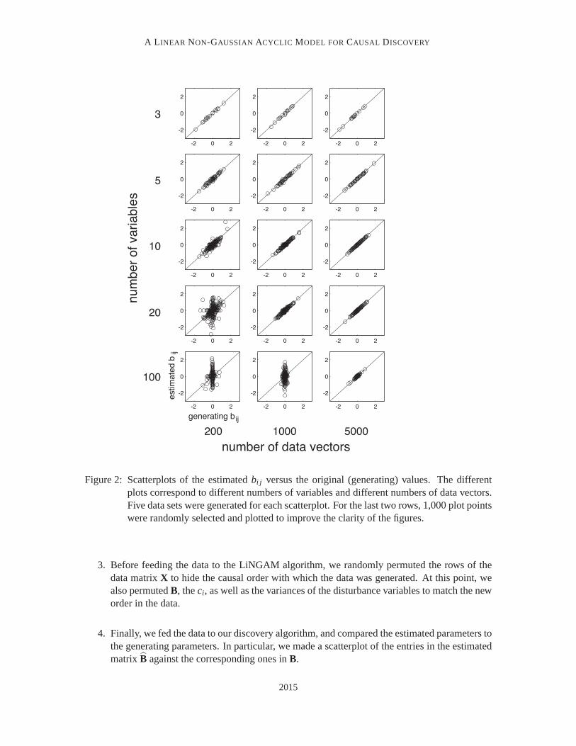
Figure 2: Scatterplots of the estimated bi j versus the original (generating) values. The differentplots correspond to different numbers of variables and different numbers of data vectors.Five data sets were generated for each scatterplot. For the last two rows, 1,000 plot pointswere randomly selected and plotted to improve the clarity of the figures.

3. Before feeding the data to the LiNGAM algorithm, we randomly permuted the rows of thedata matrix X to hide the causal order with which the data was generated. At this point, wealso permuted B, the ci, as well as the variances of the disturbance variables to match the neworder in the data.

4. Finally, we fed the data to our discovery algorithm, and compared the estimated parameters tothe generating parameters. In particular, we made a scatterplot of the entries in the estimatedmatrix B against the corresponding ones in B.

2015


Since the number of different possible parameter configurations is limitless, we feel that thereader is best convinced by personally running the simulations using various settings. Nevertheless,we here show some representative results.

Figure 2 gives combined scatterplots of the elements of B versus the generating coefficients.The different plots correspond to different dimensionalities (numbers of variables) and differentdata sizes (numbers of data vectors), where each plot combines the data for a number of differentnetwork sparseness levels and non-linearities. Although for very small data sizes the estimationoften fails, when the data size grows the estimation works practically flawlessly, as evidenced bythe grouping of the data points onto the main diagonal.

In summary, the experiments verify the correctness of the method and demonstrate that reliableestimation is possible even with fairly limited amounts of data. We note that for larger dimensionswe clearly need more data, but the amounts of data required are still reasonable.

7.2 Pruning Edges

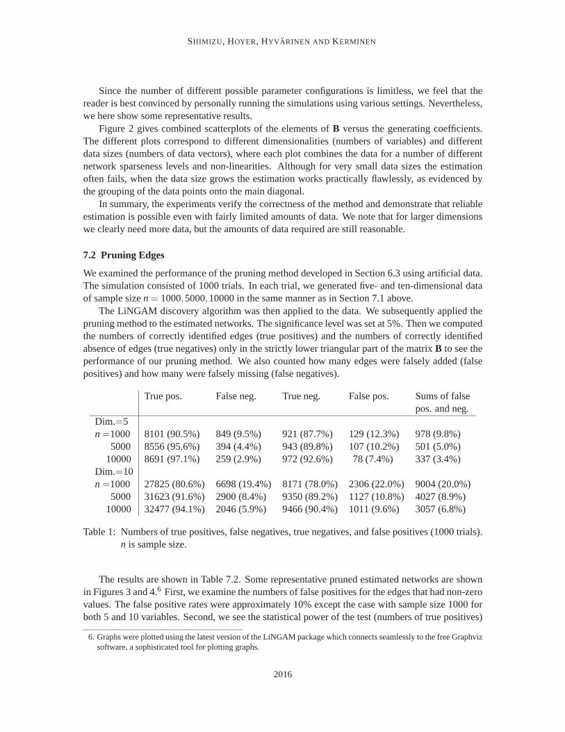
We examined the performance of the pruning method developed in Section 6.3 using artificial data.The simulation consisted of 1000 trials. In each trial, we generated five- and ten-dimensional dataof sample size n = 1000,5000,10000 in the same manner as in Section 7.1 above.

The LiNGAM discovery algorithm was then applied to the data. We subsequently applied thepruning method to the estimated networks. The significance level was set at 5%. Then we computedthe numbers of correctly identified edges (true positives) and the numbers of correctly identifiedabsence of edges (true negatives) only in the strictly lower triangular part of the matrix B to see theperformance of our pruning method. We also counted how many edges were falsely added (falsepositives) and how many were falsely missing (false negatives).

True pos. False neg. True neg. False pos. Sums of falsepos. and neg.

Dim.=5n =1000 8101 (90.5%) 849 (9.5%) 921 (87.7%) 129 (12.3%) 978 (9.8%)

5000 8556 (95.6%) 394 (4.4%) 943 (89.8%) 107 (10.2%) 501 (5.0%)10000 8691 (97.1%) 259 (2.9%) 972 (92.6%) 78 (7.4%) 337 (3.4%)

Dim.=10n =1000 27825 (80.6%) 6698 (19.4%) 8171 (78.0%) 2306 (22.0%) 9004 (20.0%)

5000 31623 (91.6%) 2900 (8.4%) 9350 (89.2%) 1127 (10.8%) 4027 (8.9%)10000 32477 (94.1%) 2046 (5.9%) 9466 (90.4%) 1011 (9.6%) 3057 (6.8%)

Table 1: Numbers of true positives, false negatives, true negatives, and false positives (1000 trials).n is sample size.

The results are shown in Table 7.2. Some representative pruned estimated networks are shownin Figures 3 and 4.6 First, we examine the numbers of false positives for the edges that had non-zerovalues. The false positive rates were approximately 10% except the case with sample size 1000 forboth 5 and 10 variables. Second, we see the statistical power of the test (numbers of true positives)

6. Graphs were plotted using the latest version of the LiNGAM package which connects seamlessly to the free Graphvizsoftware, a sophisticated tool for plotting graphs.

2016


for the other edges that had non-zero values. The power of 0.90 (8055 true positives for 5 variablesand 31071 true positives for 10 variables) was achieved for all the conditions other than when thenumber of variables was 10 and the sample size was 1000. Finally, we would mention that the sumsof the two errors (false negatives and false positives) were small enough (less than 10%) except forthe case with the number of variables 10 and the sample size 1000. Thus, Table 7.2 implied that ourpruning method worked well for reasonable sample sizes.

x1

x2

0.77

x3

0.12

x4

-0.15

x5

-1.1

-0.87 0.6

x6

0.019

-0.89 -0.43

x1

x2

0.76

x3

0.11

x4

-0.15

x5

-1.1

-0.86 0.62

x6

0.021

-0.89 -0.43

Figure 3: Left: example original network. Right: estimated network. The sample size was 10000.The structure of the original network was correctly estimated, and all the edge strengthswere approximately correct.

8. Examples With Real-World Data

As a real-world example, we have applied the LiNGAM analysis to a set of time series. As a causemust precede its effect in time, we can expect the LiNGAM analysis to find the correct time orderingof the variables in any data generated from a LiNGAM model.

A time series can be approximated by a LiNGAM model if it is a stationary AR(p) process. AnAR(p) process, or an autoregressive process of order p, is defined by the equation (Box and Jenkins,1976)

Xt = φ1Xt−1 +φ2Xt−2 + · · ·+φpXt−p +at .

That is, the value of Xt is a weighted sum of p previous variables and white noise (at). The weightsφ1,φ2, . . . ,φp are called the parameters of the process. A process is stationary, if the variance isfinite, the mean remains the same over time, and the autocovariance function depends only on thetime lag of two variables (Brockwell and Davis, 1987). The last condition also implies that thevariance remains the same over time. If we want to approximate a stationary AR(p) process by aLiNGAM model, the white noise process must be non-Gaussian.

A time series must be presented to the LiNGAM analysis as a multivariate data set. To do this,the time series is divided into time windows with the same size as the number of variables in the

2017


x1

x2

0.49

x3

0.7

x4

-1.2

x5

0.17

x6

0.0088

-0.14

0.91

0.54 0.97

-0.063

-0.12 -0.42

x7

-0.77

0.87 -0.66

x1

x2

0.48

x3

0.71

x4

-1.2

x5

0.17

x7

-0.019

-0.17

0.91

0.55 0.96

x6

-0.06

-0.13 -0.43

-0.79

0.9 -0.68

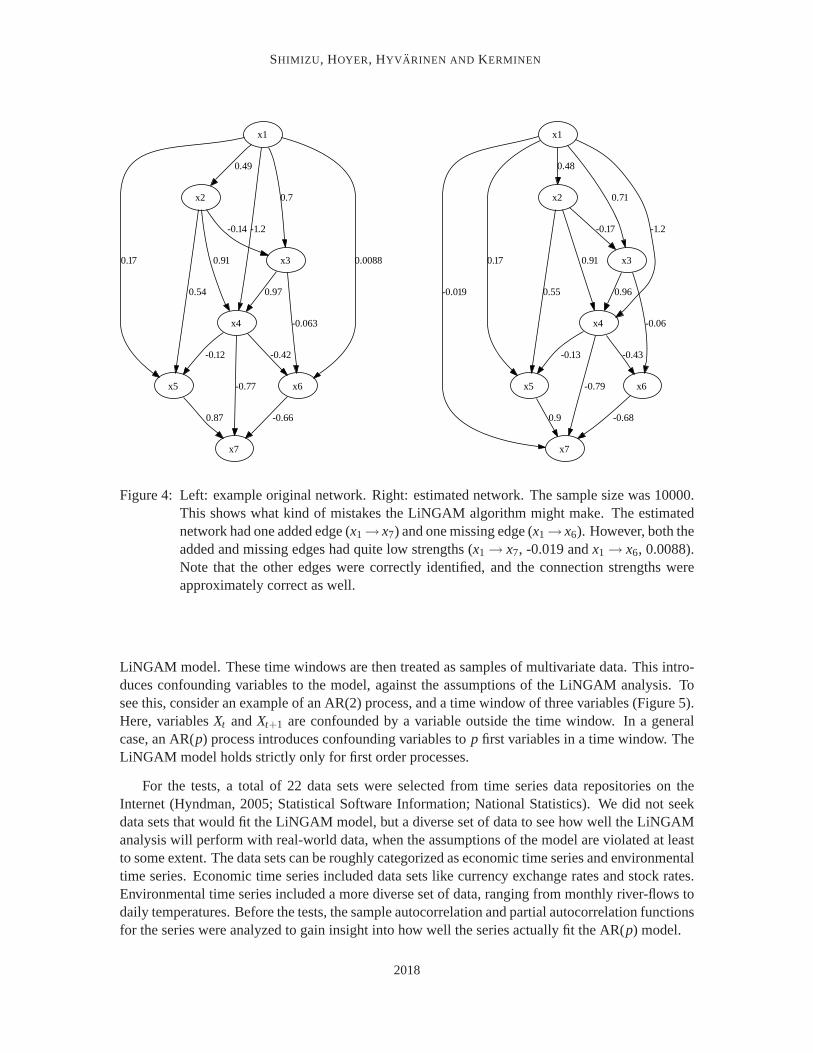
Figure 4: Left: example original network. Right: estimated network. The sample size was 10000.This shows what kind of mistakes the LiNGAM algorithm might make. The estimatednetwork had one added edge (x1 → x7) and one missing edge (x1 → x6). However, both theadded and missing edges had quite low strengths (x1 → x7, -0.019 and x1 → x6, 0.0088).Note that the other edges were correctly identified, and the connection strengths wereapproximately correct as well.

LiNGAM model. These time windows are then treated as samples of multivariate data. This intro-duces confounding variables to the model, against the assumptions of the LiNGAM analysis. Tosee this, consider an example of an AR(2) process, and a time window of three variables (Figure 5).Here, variables Xt and Xt+1 are confounded by a variable outside the time window. In a generalcase, an AR(p) process introduces confounding variables to p first variables in a time window. TheLiNGAM model holds strictly only for first order processes.

For the tests, a total of 22 data sets were selected from time series data repositories on theInternet (Hyndman, 2005; Statistical Software Information; National Statistics). We did not seekdata sets that would fit the LiNGAM model, but a diverse set of data to see how well the LiNGAManalysis will perform with real-world data, when the assumptions of the model are violated at leastto some extent. The data sets can be roughly categorized as economic time series and environmentaltime series. Economic time series included data sets like currency exchange rates and stock rates.Environmental time series included a more diverse set of data, ranging from monthly river-flows todaily temperatures. Before the tests, the sample autocorrelation and partial autocorrelation functionsfor the series were analyzed to gain insight into how well the series actually fit the AR(p) model.

2018


Figure 5: An example of confounding. Variables Xt and Xt+1 are confounded by a variable outsidethe time window.

The LiNGAM analysis was run for each data set with varying parameters. The number ofvariables in the LiNGAM model was 3, 5, or 7, corresponding to AR(p) processes of orders 2,4, and 6. Since the partial autocorrelations of economic time series indicated that the processesare at most second order processes, only models with 3 or 5 variables were tested for them. Allpossible time windows were used as multivariate data samples, including overlapping windows.For each number of variables, the LiNGAM analysis was run many times (100) to see if the analysisproduced consistent results, where initial points of FastICA algorithm were randomized to assessthe computational stability, that is, the effect of local minima.

Keeping in mind that there are possibly deviations from the LiNGAM model in the data, thereare different possible results for applying the LiNGAM analysis. If the data generating process isindeed a stationary AR(p) process with non-Gaussian noise, we can expect to find the correct timeordering of the variables. An important nonstationary process, commonly encountered in economictime series, is the random walk Xt = Xt−1 + at . If the generating process is a random walk, wecannot determine the direction of time. Hence, both the correct time ordering and the reverse timeordering are possible results. It is also possible that the variables are not causally related, and theweight matrix B is a matrix, none of which elements are significantly different from zero. In thiscase, any ordering of the variables is plausible. Also, any of the assumptions may fail to hold inreal-world data: the process might be non-linear, the error terms might have Gaussian distribution,or there might be confounding variables. In this case, the LiNGAM analysis will probably fail,producing unpredictable results.

Reflecting the possibilities explained above, four distinct categories of results were distin-guished from the tests.

1. The correct causal order was found (5 cases).

2. The reverse causal order was found (9 cases).

3. The B matrix was estimated as a zero matrix (1 case).

4. No consistent estimate for causal order was found (7 cases).

For the first three categories, the estimates were consistent over all experiments. The last categoryincluded data sets for which no consistent estimate was found. It also included some data sets forwhich a consistent estimate was found for some test setting, but not for all settings. An examplefrom each category is provided for further analysis. The examples are listed Table 2, together with

2019


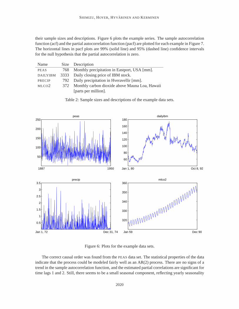
their sample sizes and descriptions. Figure 6 plots the example series. The sample autocorrelationfunction (acf) and the partial autocorrelation function (pacf) are plotted for each example in Figure 7.The horizontal lines in pacf plots are 99% (solid line) and 95% (dashed line) confidence intervalsfor the null hypothesis that the partial autocorrelation is zero.

Name Size DescriptionPEAS 768 Monthly precipitation in Eastport, USA [mm].DAILYIBM 3333 Daily closing price of IBM stock.PRECIP 792 Daily precipitation in Hveravellir [mm].MLCO2 372 Monthly carbon dioxide above Mauna Loa, Hawaii

[parts per million].

Table 2: Sample sizes and descriptions of the example data sets.

1887 1950

50

100

150

200

250peas

Jan 1, 80 Oct 8, 92

60

80

100

120

140

160

180dailyibm

Jan 1, 72 Dec 31, 74

0.5

1

1.5

2

2.5

3

3.5precip

Jan 59 Dec 90

320

330

340

350

360mlco2

Figure 6: Plots for the example data sets.

The correct causal order was found from the PEAS data set. The statistical properties of the dataindicate that the process could be modeled fairly well as an AR(2) process. There are no signs of atrend in the sample autocorrelation function, and the estimated partial correlations are significant fortime lags 1 and 2. Still, there seems to be a small seasonal component, reflecting yearly seasonality

2020


of precipitation. The most frequent model estimated by LiNGAM was an AR(2) process with smallparameters, in accordance with the estimated partial correlations.

The reverse causal order was found from the DAILYIBM data set. The acf and the pacf of thedata resemble those of a random walk, thus the result is expected. Also the estimated causal modelis close to a random walk, values of nearly one are estimated consistently for the first parameter ofthe AR(p) process, other weight estimates being zero.

5 10 15 20 25 30 35 40−0.5

0

0.5

1acf, peas

1 5 10 15 20−0.2

0

0.2pacf, peas

200 400 600 800−0.5

0

0.5

1acf, dailyibm

1 5 10 15 20−1

−0.5

0

0.5pacf, dailyibm

5 10 15 20 25 30 35 40−0.5

0

0.5

1acf, precip

1 5 10 15 20−0.1

0

0.1pacf, precip

20 40 60 800

0.5

1acf, mlco2

1 5 10 15 20−1

−0.5

0

0.5pacf, mlco2

Figure 7: The sample autocorrelation and partial autocorrelation functions for the example datasets.

For the PRECIP data set, the estimates for causal order were consistent, but not consistentlyeither correct or reverse. Most of the time, the estimated B matrix was a zero matrix. As a zero Bmatrix is consistent with any time ordering of the variables, this largely explains the results. For thecases when the B matrix was not a zero matrix, the estimated weights were small (less than 0.1),and did not correspond to an AR(p) model of any order, but rather random estimation errors. Thepacf of this series supports the results of the LiNGAM analysis: none of the partial autocorrelationsis statistically significant.

For the MLCO2 data set, the LiNGAM analysis produced inconsistent estimates of the causalorder. There are several possible reasons for this. First of all, the series has a trend and a seasonal

2021


component. More probably, the basic assumptions of the LiNGAM analysis are violated. Theprocess might be non-linear, or the level of carbon dioxide might be caused by other environmentalvariables, leading to a confounded model. It is also possible, although unlikely, that the data isGaussian.

9. Conclusions

Developing methods for causal inference from non-experimental data is a fundamental problemwith a very large number of potential applications. Although one can never fully prove the validityof a causal model from observational data alone, such methods are nevertheless crucial in caseswhere it is impossible or very costly to perform experiments.

Previous methods developed for linear causal models (Bollen, 1989; Spirtes et al., 2000; Pearl,2000) have been based on an explicit or implicit assumption of Gaussianity, and have hence beenbased solely on the covariance structure of the data. Because of this, additional information (suchas the time-order of the variables) is usually required to obtain a full causal model of the variables.Without such information, algorithms based on the Gaussian assumption cannot in most cases dis-tinguish between multiple equally possible causal models.

In this paper, we have shown that an assumption of non-Gaussianity of the disturbance variables,together with the assumption of linearity and causal sufficiency, allows the causal model to becompletely identified. Furthermore, we have proposed a practical algorithm which estimates thecausal structure under these assumptions and provided a number of tests to prune the graph and tosee whether the estimated model fits the data.

The practical value of the LiNGAM analysis needs to be determined by applying it to real-worlddata sets and comparing it to other methods for causal inference from non-experimental data. Thereal data examples reported here are rather limited. Also, in many cases involving real-world data,practitioners in the field already have a fairly good understanding of the causal processes underlyingthe data. An interesting question is how well methods such as ours do on such data sets. These areimportant topics for future work.

Acknowledgments

This work was partially carried out at Division of Mathematical Science, Graduate School of En-gineering Science, Osaka University and Transdisciplinary Research Integration Center, ResearchOrganization of Information and Systems. The authors would like to thank Aristides Gionis, HeikkiMannila, and Alex Pothen for discussions relating to algorithms for solving the permutation prob-lems, Niclas Borlin for contributing the Matlab code for solving the assignment problem, YutakaKano and Michiwo Kanekiyo for comments on the manuscript and Michael Jordan and three anony-mous reviewers for useful comments to improve this paper. S.S. was supported by Grant-in-Aid forScientific Research from Japan Society for the Promotion of Science. P.O.H. was supported by theAcademy of Finland project #204826. A.H. was supported by the Academy of Finland through anAcademy Research Fellow Position and project #203344.

2022


Appendix A. Proof of Uniqueness of Row Permutation

Here, we show that, were the estimates of ICA exact, there is only a single permutation of the rowsof W which results in a diagonal with no zero entries.

It is well-known (Bollen, 1989) that the DAG structure of the network guarantees that for somepermutation of the variables, the matrix B is strictly lower-triangular. This implies that the correctW (where the disturbance variables are aligned with the observed variables) can be permuted tolower-triangular form (with no zero entries on the diagonal) by equal row and column permutations,that is,

W = PdMPTd ,

where M is lower-triangular and has no zero entries on the diagonal, and Pd is a permutation matrixrepresenting a causal ordering of the variables. Now, ICA returns a matrix with randomly permutedrows,

W = PicaW = PicaPdMPTd = P1MPT

2 ,

where Pica is the random ICA row permutation, and on the right we have denoted by P1 = PicaPd

and P2 = Pd , respectively, the row and column permutations from the lower triangular matrix M.We now prove that W has no zero entries on the diagonal if and only if the row and column

permutations are equal, that is, P1 = P2. Hence, there is only one row permutation of W whichyields no zero entries on the diagonal, and it is the one which finds the correspondence between thedisturbance variables and the observed variables.

Lemma 1 Assume M is lower triangular and all diagonal elements are non-zero. A permutation ofrows and columns of M has only non-zero entries in the diagonal if and only if the row and columnpermutations are equal.

Proof First, we prove that if the row and columns permutations are not equal, there will be zeroelements in the diagonal.

Denote by K a lower triangular matrix of all ones in the lower triangular part. Denote by P1 andP2 two permutation matrices. The number of non-zero diagonal entries in a permuted version of Kis tr(P1KPT

2 ). This is the maximum number of non-zero diagonal entries when an arbitrary lowertriangular matrix is permuted.

We have tr(P1KPT2 ) = tr(KPT

2 P1). Thus, we can consider permutations of columns only, givenby PT

2 P1. Assume the columns of K are permuted so that the permutation is not equal to identity.Then, there exists an index i so that the column of index i has been moved to column index jwhere j < i (If there were no such columns, all the columns would be moved to the right, which isimpossible.) Obviously, the diagonal entry in the j-th column in the permuted matrix is zero. Thus,any column permutation not equal to the identity creates at least one zero entry in the diagonal.

Thus, to have non-zero diagonal, we must have PT2 P1 = I. This means that the column and row

permutations must be equal.Next, assume that the row and column permutations are equal. Consider M = I as a worst-

case scenario. Then the permuted matrix equals P1IPT2 which equals identity, and all the diagonal

elements are non-zero. Adding more non-zero elements in the matrix only increases the number ofnon-zero elements in the permuted version.

Thus, the lemma is proven.

2023


Appendix B. An Example of the Permutation Problem

Here we show with an example that if the permutation is not correctly determined, the parametersbi j can have very different values, yet give the same data distribution. This example considers thegeneral case where the system is not DAG. For simplicity, let us consider the two variables case.Assume we parameterize the mixing model in (2) as[

x1

x2

]=

11−b12b21

[1 b12

b21 1

]diag(σ1,σ2)

[s1

s2

],

where σ1 and σ2 are standard deviations of e1 and e2, and s1 and s2 are normalized versions of e1

and e2, that is, e1/σ1 and e2/σ2.Then, take the following new set of parameters:

b′12 = 1/b21

b′21 = 1/b12

σ′1 = σ2/b21

σ′2 = σ1/b12,

and do the permutation and sign change:

s′1 = −s2

s′2 = −s1.

Then, the two parameterizations give the same data, that is, the same model fit. This is because

11−b′12b′21

[1 b′12

b′21 1

]diag(σ′

1,σ′2)

[s′1s′2

]=

11−1/(b12b21)

[1 1/b21

1/b12 1

]diag(σ2/b21,σ1/b12)

[ −s2

−s1

]=

−b12b21

1−b12b21

[1/b21 1/(b21b12)

1/(b12b21) 1/b12

]diag(σ2,σ1)

[ −s2

−s1

]=

b12b21

1−b12b21

[1/b21 1/(b21b12)

1/(b12b21) 1/b12

]diag(σ2,σ1)

[s2

s1

]=

11−b12b21

[b12 11 b21

]diag(σ2,σ1)

[s2

s1

]=

11−b12b21

[1 b12

b21 1

]diag(σ1,σ2)

[s1

s2

].

Therefore, the parameter sets with or without “prime” are equivalent. The model fit is the samewith two different sets of parameters. Estimation of the model can equally well give any of thesetwo sets. However, the numerical values of b and b′ are quite different. In this example, the systemwas not constrained to be a DAG. In fact, if the original system is a DAG, the system with primeshas infinite coefficients. Thus, we see how the constraint of DAG is helpful.

2024


Appendix C. ML Derivation of Objective Function for Finding the Correct RowPermutation

Since the ICA estimates are never exact, all elements of W will be non-zero, and one cannot basethe permutation on exact zeros. Here we show that the objective function for step 2 of the LiNGAMalgorithm can be derived from a maximum likelihood framework.

Let us denote by eit the value of disturbance variable i for the t-th data vector of the data set.Assume that we model the disturbance variables eit by a generalized Gaussian density:

log p(eit) = −|eit |α/β+Z,

where the α,β are parameters and Z is a normalization constant. Then, the log-likelihood of themodel equals

∑t

∑i

−1β

∣∣∣∣ eit

wii

∣∣∣∣α= −∑

i

1β|wii|α ∑

t|eit |α,

because each row of W is subsequently divided by its diagonal element. To maximize the likelihood,we find the permutation of rows for which the diagonal elements maximize this term. For simplicity,assuming that the pdf’s of all independent components are the same, this means we solve

minall row perms

∑i

1|wii|α .

In principle, we could estimate α from the data using ML estimation as well, but for simplicity wefix it to unity because it does not really change the qualitative behavior of the objective function.Regardless of its value, this objective function heavily penalizes small values on the diagonal, as weintuitively (based on the argumentation in Section 4) require.

Appendix D. Asymptotic Variance of ICA

Several authors studied asymptotic variance of ICA (Pham and Garrat, 1997; Hyvarinen, 1997; Car-doso and Laheld, 1996; Tichavsky et al., 2006), where the theory of estimating functions (Godambe,1991) was often used. Let us consider a semiparametric model p(x|θ), where θ is a r-dimensionalparameter vector of interest. Note that the density function p(x|θ) is unknown. Let us denote byθ0 the true parameter vector of interest. A r-dimensional vector-valued function f (x,θ) is called anestimating function when it satisfies the following conditions for any p(x|θ0):

E[ f (x,θ0)] = 0

|det J| = 0, where J = E

[∂

∂θT f (x,θ)∣∣∣∣θ=θ0

]E[‖ f (x,θ0)‖2] < ∞,

where the expectation E is taken over x with respect to p(x|θ0).Let x(1), · · · ,x(n) be a random sample from p(x|θ0). Then an estimator θ is obtained by solving

the estimating equation:

n

∑i=1

f (x(i),θ) = 0.

2025


Under some regularity conditions including identification conditions for θ, the estimator θ is con-sistent when n goes to infinity and asymptotically distributes according to the Gaussian distributionN(θ0,G), and

G =1n

J−1E[ f (x,θ0) f T (x,θ0)]J−T . (5)

Pham and Garrat (1997) derived an estimating function for (quasi-) maximum likelihood es-timation. Kawanabe and Muller (2005) provided estimating functions for JADE (Cardoso andSouloumiac, 1993) and for ICA based on non-Gaussianity maximization with orthogonality (un-correlatedness) constraints including FastICA (Hyvarinen, 1999).

In this paper, we restrict ourselves to testing mixing and demixing coefficients estimated byFastICA. In the FastICA, we first center the data to make its mean zero and whiten the data bycomputing a matrix V such that the covariance matrix of z = Vx is the identity matrix. After that, wefind an orthogonal matrix Q so that components of QT z = QT Vx have maximum non-Gaussianity.Then we obtain estimates of A and W by A = V−1Q and W = QT V.

Let us consider the following function:

F(x,Q) = yyT − I+ ygT (y)−g(y)yT ,

where y = Wx = QT Vx = QT z and g(u) is the non-linearity. The estimating function for FastICAis obtained as f = vec(F) taking θ = vec(Q) (Kawanabe and Muller, 2005). Here, vec(·) denotesthe vectorization operator which creates a column vector from a matrix by stacking its columns.

According to the estimating function theory, we obtain the asymptotic covariance matrix ofvec(Q) by (5). Here we assume that the variance in the estimate of V is negligible with respectto the variance in Q. Then we obtain the asymptotic covariance matrix of vec(A) and vec(W) asfollows:

acov{vec(A)} = acov{vec(V−1Q)}= (I⊗V−1)acov{vec(Q)}(I⊗V−1)T

acov{vec(W)} = acov{vec(QT V)}= (VT ⊗ I)acov{vec(QT )}(VT ⊗ I)T ,

where ⊗ denotes the Kronecker product.7

The formula of acov{vec(Q)} for FastICA is written as

acov{vec(Q)} =1n

J−1E[vec{F(x,Q)}vec{F(x,Q)}T ]J−T .

Let us denote by Fpq and Fq the (p,q)-element and the q-th column of F, respectively. We shallprovide E(FpqFrs) to compute E{vec(F)vec(F)T}. Denote by i, j,k, l four different subscripts. Then

7. The Kronecker product Y⊗Z of matrices Y and Z is defined as a partitioned matrix with (i, j)-th block equal to yi jZ.

2026


we have

E(FiiFii) = E(s4i )+1, E(FiiFj j) = 2, E(FkiFi j) = −E{g(sk)}E{g(s j)}

E(FkiFli) = E{g(sk)}E{g(sl)}, E(FkiFk j) = E{g(si)}E{g(s j)}E(FiiFli) = −E(s3

i )E{g(sl)}, E(FkiFii) = −E(s3i )E{g(sk)}

E(FiiFi j) = E(s3i )E{g(s j)}, E(FjiFj j) = E(s3

j)E{g(si)}E(FiiFl j) = 0, E(FkiFj j) = 0, E(FkiFl j) = 0

E(FjiFi j) = 1+2E{sig(si)}E{s jg(s j)}−E{g(si)2}−E{g(s j)2}E(FjiFl j) = 1+E{sig(si)}+E{s jg(s j)}+E{sig(si)}E{s jg(s j)}−E{g(si)}E{g(sl)}E(FkiFki) = 1+2E{sig(si)}−2E{skg(sk)}+E{g(si)2}+E{g(sk)2}

−2E{sig(si)}E{skg(sk)}.

Further we shall give E{

(∂Fi)/(∂qTj )

}to compute J = E

[{∂vec(F)}/{∂vec(Q)T}]:E

[∂Fi

∂qTi

]=

{2E(qT

i zzT )E{qT

k zzT − zT g(qTk z)+qT

k zg′(qTi z)zT}

={

2qTi (i−th row)

[1−E{skg(sk)}+E{g′(si)}]qTk (k−th row, k = i)

E

[∂Fi

∂qTj

]=

{E[{1−g′(qT

j z)}qTi zzT + zT g(qT

i z)]0T

={

[1−E{g′(s j)}+E{sig(si)]qTi ( j−th row, j = i)

0T (k−th row, k = j).

Appendix E. Exact Form of J = ∂σ2(τ)/∂τT

We here derive the exact form of J = ∂σ2(τ)/∂τT in (4). Let us denote by Σ2 the covariance matrixbased on the model or E(xxT ). The σ2(τ) in (3) is obtained by vec+(Σ2). Let us rewrite theLiNGAM model as:

x = (I−B)−1e

= (I−B)−1D12 e,

where D = cov(e) and e = D− 12 e. Note that E(e) = 0 is assumed. Then the model-based covariance

matrix Σ is:

Σ = (I−B)−1D12 cov(e)D

12 (I−B)−T

={

D− 12 (I−B)

}−1 {D− 1

2 (I−B)}−T

= YYT ,

where

Y ={

D− 12 (I−B)

}−1.

2027


Now we need to compute the following derivatives:

∂Σi j

∂bkl=

∂(YYT )i j

∂bkl= ∑

p∑q

∂(YYT )i j

∂Ypq

∂Ypq

∂bkl

∂Σi j

∂dkk=

∂(YYT )i j

∂dkk= ∑

p∑q

∂(YYT )i j

∂Ypq

∂Ypq

∂dkk.

We provide ∂(YYT )i j/∂Ypq, ∂Ypq/∂bkl , and ∂Ypq/∂dkk to compute the derivatives above:

∂(YYT )i j

∂Ypq=

⎧⎪⎪⎨⎪⎪⎩2Ypq (i = p, j = p)Y jq (i = p, j = p)Yiq (i = p, j = p)0 (i = p, j = p)

∂Y∂bkl

= −Y∂Y−1

∂bklY

= YD− 12 JklY

∂Y∂dkk

= −Y∂Y−1

∂dkkY

= Yd−3/2

kk

2Jkk(I−B)Y,

where Jkl is the single-entry matrix with 1 at (k, l) and zero elsewhere. Thus, we can computeJ = ∂σ2/∂τT = ∂vec+(Σ2)/∂τT .

References

Y. Benjamini and Y. Hochberg. Controlling the false discovery rate: a practical and powerful ap-proach to multiple testing. Journal of the Royal Statistical Society: Series B, 57:289–300, 1995.

K. A. Bollen. Structural Equations with Latent Variables. John Wiley & Sons, 1989.

G. E. P. Box and G. M. Jenkins. Time Series Analysis: forecasting and control. Holden-Day,Oakland, California, USA, revised edition, 1976.

P. J. Brockwell and R. A. Davis. Time Series: Theory and Methods. Springer-Verlag, New York,USA, 1987.

M. W. Browne. Asymptotically distribution-free methods for the analysis of covariance structures.British Journal of Mathematical and Statistical Psychology, 9:665–672, 1984.

R. E. Burkard and E. Cela. Linear assignment problems and extensions. In P. M. Pardalos and D. Z.Du, editors, Handbook of Combinatorial Optimization - Supplement Volume A, pages 75–149.Kluwer, 1999.

J.-F. Cardoso and B. H. Laheld. Equivariant adaptive source separation. IEEE Trans. on SignalProcessing, 44:3017–3030, 1996.

2028


J.-F. Cardoso and A. Souloumiac. Blind beamforming for non Gaussian signals. IEE Proceedings-F,140(6):362–370, 1993.

P. Comon. Independent component analysis – a new concept? Signal Processing, 36:287–314,1994.

Y. Dodge and V. Rousson. On asymptotic properties of the correlation coefficient in the regressionsetting. The American Statistician, 55(1):51–54, 2001.

B. Efron and R. Tibshirani. An Introduction to the Bootstrap. Chapman & Hall, New York, 1993.

D. Geiger and D. Heckerman. Learning gaussian networks. In Proceedings of the 10th AnnualConference on Uncertainty in Artificial Intelligence (UAI-94), pages 235–243, 1994.

V. P. Godambe. Estimating functions. Oxford University Press, New York, 1991.

J. Himberg, A. Hyvarinen, and F. Esposito. Validating the independent components of neuroimagingtime-series via clustering and visualization. Neuroimage, 22:1214–1222, 2004.

Y. Hochberg. A sharper Bonferroni procedure for multiple tests of significance. Biometrika, 4:800–802, 1988.

Y. Hochberg and A. C. Tamhane. Multiple comparison procedures. John Wiley & Sons, New York,1987.

S. Holm. A simple sequentially rejective multiple test procedure. Scandinavian Journal of Statistics,6:65–70, 1979.

P. O. Hoyer, S. Shimizu, A. Hyvarinen, Y. Kano, and A. J. Kerminen. New permutation algorithmsfor causal discovery using ICA. In Proceedings of International Conference on IndependentComponent Analysis and Blind Signal Separation, Charleston, SC, USA, pages 115–122, 2006a.

P. O. Hoyer, S. Shimizu, and A. J. Kerminen. Estimation of linear, non-gaussian causal models in thepresence of confounding latent variables. In Proc. the third European Workshop on ProbabilisticGraphical Models (PGM2006), 2006b. In press.

L. Hu, P. M. Bentler, and Y. Kano. Can test statistics in covariance structure analysis be trusted?Psychological Bulletin, 112:351–362, 1992.

R. J. Hyndman. Time series data library, 2005. URL http://www-personal.buseco.monash.edu.au/˜hyndman/TSDL/. [June 2005].

A. Hyvarinen. One-unit contrast functions for independent component analysis: A statistical anal-ysis. In Neural Networks for Signal Processing VII (Proceedings of IEEE Workshop on NeuralNetworks for Signal Processing), pages 388–397, 1997.

A. Hyvarinen. Fast and robust fixed-point algorithms for independent component analysis. IEEETrans. on Neural Networks, 10(3):626–634, 1999.

A. Hyvarinen, J. Karhunen, and E. Oja. Independent Component Analysis. Wiley Interscience,2001.

2029


M. Kawanabe and K. R. Muller. Estimating functions for blind separation when sources havevariance dependencies. Journal of Machine Learning Research, 6:453–482, 2005.

National Statistics, 2005. URL http://www.statistics.gov.uk/. [June 2005].

J. Pearl. Causality: Models, Reasoning, and Inference. Cambridge University Press, 2000.

D. T. Pham and P. Garrat. Blind separation of mixture of independent sources through a quasi-maximum likelihood approach. Signal Processing, 45:1457–1482, 1997.

S. Shimizu, A. Hyvarinen, P. O. Hoyer, and Y. Kano. Finding a causal ordering via independentcomponent analysis. Computational Statistics & Data Analysis, 50(11):3278–3293, 2006a.

S. Shimizu, A. Hyvarinen, Y. Kano, and P. O. Hoyer. Discovery of non-gaussian linear causalmodels using ICA. In Proc. the 21st Conference on Uncertainty in Artificial Intelligence (UAI-2005), pages 526–533, 2005.

S. Shimizu, A. Hyvarinen, Y. Kano, P. O. Hoyer, and A. J. Kerminen. Testing significance of mixingand demixing coefficients in ICA. In Proceedings of International Conference on IndependentComponent Analysis and Blind Signal Separation, Charleston, SC, USA, pages 901–908, 2006b.

S. Shimizu and Y. Kano. Use of non-normality in structural equation modeling: Application todirection of causation. Journal of Statistical Planning and Inference, 2006. In press.

R. J. Simes. An improved Bonferroni procedure for multiple tests of significance. Biometrika, 73:751–754, 1986.

P. Spirtes, C. Glymour, and R. Scheines. Causation, Prediction, and Search, 2nd ed. MIT Press,2000.

Statistical Software Information, 2005. URL http://www-unix.oit.umass.edu/˜statdata/.[June 2005].

P. Tichavsky, Z. Koldovsky, and E. Oja. Performance analysis of the FastICA algorithm andCramer-Rao bounds for linear independent component analysis. IEEE Trans. on Signal Pro-cessing, 54(4):1189–1203, 2006.

K-H. Yuan and P. M. Bentler. Mean and covariance structure analysis: Theoretical and practicalimprovements. Journal of the American Statistical Association, 92(438):767–774, 1997.

2030

Documents

A Linear Non-Gaussian Acyclic Model for Causal …A Linear Non-Gaussian Acyclic Model for Causal Discovery Shohei Shimizu∗ [email protected] JP Patrik O. Hoyer PATRIK.HOYER@HELSINKI