A Lifecycle Model with Human Capital, LaborSupply and Retirement

(Preliminary and Incomplete)

Xiaodong FanUniversity of New South Wales

Ananth SeshadriUniversity of Wisconsin-Madison

Christopher TaberUniversity of Wisconsin-Madison

May 15, 2014

Abstract

We develop and estimate a Ben-Porath human capital model in which individuals makedecisions on consumption, human capital investment, labor supply, and retirement. Themodel allows for both an endogenous wage process (which is typically assumed exoge-nous in the retirement literature) and an endogenous retirement decision (which is typi-cally assumed exogenous in the human capital literature). We estimate the model usingthe Method of Simulated Moments to match the life-cycle profiles of wages and hoursfrom the SIPP data. The model replicates the main features of the data.

KEYWORDS: human capital, Ben-Porath, labor supply, retirementJEL Classification: J22, J24, J26

1. Introduction

The Ben-Porath (1967) model of lifecycle human capital production and the lifecycle labor

supply model are two of the most important models in labor economics. While the for-

mer is the dominant framework used to rationalize wage growth over the life-cycle, the

latter has been used to study hours worked over the life-cycle. Quite surprisingly, aside

from the seminal work in Heckman (1976) there has been little effort integrating these

two important paradigms. This paper attempts to fill this void by estimating a lifecycle

model in which workers make human capital and labor supply decisions jointly. Work-

ers acquire human capital on the job. Perhaps the most important aspect of our model is

that we do not treat retirement as a separate decision. It occurs endogenously as part of

the optimal lifecycle labor supply profile. While most work to date on the lifecycle hu-

man capital model aims to explain the wage growth early in the lifecycle, there has been

surprisingly little work combining human capital with labor supply and retirement. We

estimate a model that is rich enough to explain both the lifecycle pattern of wages as well

as the lifecycle pattern of labor supply-focusing on retirement and wage patterns at the

end of working life.

The retirement literature typically takes the wage process as given and estimates the

date of retirement. One typically sees wages fall substantially before retirement. Raw

wages for people who work fall by over 25% between ages 55 and 65. In the retirement

literature, this trend is critical in explaining retirement behavior. Lifecycle human capital

models provide a very different perspective. They take the retirement date as given, but

model the formation of the wage process. We merge these two literatures by allowing

for both endogenous retirement and an endogenous wage process. In addition, we also

incorporate health shocks to investigate their importance in retirement decisions. While

most work to date on the lifecycle human capital model aims to explain the wage growth

early in the lifecycle, there has been surprisingly little work combining human capital

with labor supply wherein the labor supply, wage and retirement choices are rationalized

in one unified setting.

Specifically, we develop and estimate a Ben-Porath type human capital model in

which workers make consumption, human capital investment, and labor supply deci-

sions. We estimate the model using the Method of Simulated Moments (MSM), matching

the wage and hours profiles from the Survey of Income and Program Participation

1

(SIPP). With a parsimonious lifecycle model in which none of the parameters explicitly

depend upon age or experience, we are able to replicate the main features of the data. In

particular we match the large increase in wages and very small increase in labor supply

at the beginning of the lifecycle as well as the small decrease in wages but very large

decrease in labor supply at the end of the lifecycle. The key to our ability to fit both parts

of the lifecycle is human capital depreciation. In a simple model without human capital

or depreciation, there would be no a priori reason for workers to concentrate their leisure

at the end of the lifecycle. However, as soon as we bring in the possibility that human

capital might depreciate, this is no longer the case. If workers take time off in the middle

of their career, their human capital will fall substantially and they will make much less

when they return to the labor market. However, if this period of nonworking occurs at

the end of the career this is no longer the case. Another way to see the same point is that

if a middle age worker stops working for a while, they will generally return to the labor

market and build up their wages. However, as a result of the shorter time horizon, it

might not be worth it for an older worker to re-enter at a lower wage so they continue

to stay out of the labor market. Allowing for exogenous human capital accumulation

across the lifecycle without depreciation will not be enough to explain the patterns. If

the tastes for leisure does not vary across the labor market the standard model cannot

simultaneously reconcile the small increase in labor supply and large increase in wages

at the beginning of the lifecycle and the small decrease in wages and large decrease in

labor supply at the end. Of course if one exogenously allowed both wages and labor

supply to depend upon age in a completely flexible way one could easily fit the joint

pattern. Moreover, it is not clear that this model would have any testable implications so

we cannot reject it. The goal of this paper is to try to fit the profiles without resorting to

arbitrary taste preferences and exogenous wage variation.

An interesting aspect of our model is that even though the preference for leisure does

not vary systematically over the lifecycle, we do find that measured “labor supply elastic-

ities” do vary over the lifecycle. In our dynamic model, the shadow cost of not working

much higher early in the lifecycle (as pointed out by Imai and Keane, 2004) but in our

model it is also lower for older workers as opposed to peak earners. We find that early

in the lifecycle the measured labor supply elasticity is low for younger workers, around

0.3. However, workers around standard retirement age are more sensitive to wage fluc-

2

tuations with elasticities around 0.8. Once the model has been estimated, we can use it

to measure the impacts of Social Security policy. The U.S. government currently faces

a huge debt and it is no understatement to say that addressing this problem is one of

the primary issues facing policy makers in Washington. Moreover, with the aging of the

baby boom generation this problem is going to get worse. The amount that we spend

on Social Security and Medicare is not sustainable without major increases in funding for

them. Given this, many programs have been proposed to address these problems and

eventually something must be done.

Much serious work has been developed to quantitatively estimate the economic con-

sequences of aging population and evaluate the remedy policies (Rust and Phelan, 1997;

French, 2005; French and Jones, 2011). Haan and Prowse (2012) directly estimate the effect

of increasing life expectancy on retirement decisions. They model retirement as a result

of declining wages and increasing actuarial unfairness of the Social Security and pension

system. However, from our model one can see that there is a major issue in the previous

retirement literature. They typically take the wage process as given and focus on the re-

tirement itself. For example, when conducting the counterfactual experiment of delaying

Social Security Normal Retirement Age (NRA) from age 65 to age 67, all previous litera-

ture takes the same age-wage profile as in the baseline model where the NRA is at age 65

and re-estimates the retirement behavior under the new environment where the NRA is

67.

As the wage has already been declining significantly approaching the previous NRA

of 65, under the new policy of NRA at 67 working is not likely attractive for many workers

since the wage further declines between age 65 and 67. This decline is taken as exogenous

in these models. However, if one is expecting a NRA at age 67 instead of age 65 and

retiring later is optimal, then she or he will certainly try to keep the wage high during the

extra working time. Omitting such channel will likely generate bias in the counterfactual

policy experiments. In our counterfactual policy experiments, we find that removing the

Social Security earnings test between age 62 and 70 would lead to an average 2% decline

in wages within that age range, and that delaying the NRA two years (from age 65 to

67) would result an average 2% increase in wages at old ages. The changes in wages

are much higher in the experiments of removing the Social Security system or extending

the life expectancy. Clearly, omitting the human capital investment channel will bias the

3

results otherwise.

The remainder of the paper is organized as follows. Section 2 reviews relevant litera-

ture in human capital models and retirement. Section 3 develops the Ben-Porath model

with labor supply and retirement. Section 4 describes the estimation strategy and data.

Section 5 presents parameter estimates in the baseline model matching the SIPP data. Sec-

tion 6 discusses model implications and Section 7 simulates the effects of several policies.

Section 8 concludes.

2. Relevant Literature

(This section is rough and incomplete)

There is a large and growing literature on many aspects of retirement. In these mod-

els, typically retirement is induced either by increasing utility toward leisure (Gustman

and Steinmeier, 1986) or similarly increasing disutility toward labor supply (Blau, 2008).

Gustman and Steinmeier (2006) and Gustman and Steinmeier (2009) estimate the impact

of Social Security policies on retirement in structural models with increasing utility to-

ward leisure. Haan and Prowse (2012) estimate the extent to which the increase in life

expectancy affects retirement. Blau (2008) evaluates the role of uncertain retirement ages

in the retirement-consumption puzzle.

Retirement can also be induced by declining wages at old ages and/or fixed costs

of working. Rust and Phelan (1997) estimate a dynamic life-cycle labor supply model

with endogenous retirement decisions to study the effect of Social Security and Medicare

in retirement behavior. French (2005) estimates a more comprehensive model including

saving to study the effect of Social Security and pension as well as health in retirement

decisions. French and Jones (2011) evaluate the role of health insurance in shaping re-

tirement behavior. Casanova (2010) studies the joint retirement decision among married

couples. Prescott et al. (2009) and Rogerson and Wallenius (2010) present models where

retirement could be induced by a convex effective labor function or fixed costs.

In all the literature listed above—theoretical or empirical, the wage process is assumed

to be exogenous. That is, even when the environment changes while conducting counter-

factual experiments, for example changing the Social Security policies, the wage process

is kept the same and only the response in the retirement timing is studied.

On the other hand, human capital models have been accepted widely to explain the

4

life-cycle wage growth as well as the labor supply and income patterns. In his seminal pa-

per, Ben-Porath (1967) develops the human capital model with the idea that individuals

invest in their human capital "up front." In what follows we use the two terms—"human

capital model" and "Ben-Porath model" —interchangeably. Heckman (1976) further ex-

tends the model and presents a more general human capital model where each individ-

ual makes decisions on labor supply, investment and consumption. In both papers, each

individual lives for finite periods and the retirement age is fixed. In their recent paper,

Manuelli et al. (2012) extend the Ben-Porath model to include the endogenous retirement

decision. All three theoretical models are deterministic.

Relative to the success in theory, there hasn’t been as much work empirically estimat-

ing the Ben-Porath model. Mincer (1958) derives an approximation of the Ben-Porath

model and greatly simplifies the estimation with a quadratic in experience, which is used

in numerous empirical papers estimating the wage process (Heckman et al., 2006, survey

the literature). Early work on explicit estimation of the Ben-Porath model was done by

Heckman (1976); Haley (1976), and Rosen (1976). Heckman et al. (1998) is a more recent

attempt to estimate the Ben-Porath model. They utilize the implication of the standard

Ben-Porath model where at old ages the investment is almost zero. However, this impli-

cation does not hold any more when the retirement is uncertain, where each individual

always has incentive to invest a positive amount in human capital. Other more recent

work includes Taber (2002) who incorporates progressive income taxes into the estima-

tion and Kuruscu (2006) who estimates the model nonparametrically. Browning et al.

(1999) survey much of this literature.

Another type of human capital model, the learning-by-doing model, draws relatively

more attention in the empirical work. In the learning-by-doing model human capital

accumulates exogenously as long as an individual works-thus they only impact their

human capital accumulation through the work decision. In these models the total return

from labor supply is not only the direct wage income at current time, but also includes all

the extra wage income from the augmented human capital in all future time. Shaw (1989)

is among the first to empirically estimate the learning-by-doing model, using the PSID

model and utilizing the Euler equations on consumption and labor supply with translog

utility. Keane and Wolpin (1997) and Imai and Keane (2004) are two examples of many

that directly estimate a dynamic life-cycle with learning-by-doing. These papers assume

5

an exogenously fixed retirement age. Wallenius (2009) points out that such a learning-by-

doing model does not fit the pattern of wages and hours well at old ages.

3. Model

We present and estimate a Ben-Porath human capital model with endogenous labor sup-

ply and retirement in which individuals make decisions on consumption, human capital

investment, and labor supply (including retirement as a special case). For simplicity we

suppress the individual subscript i for all variables.

3.1 Set-up

Each individual lives from period t0 to T. One period is defined as one year. At the

beginning of the first period, each individual is endowed with an initial asset At0 ∈ R,

human capital level Ht0 ∈ R+ and health status St0 ∈ {0, 1} with 1 being in good health

and 0 in bad health.

The health status evolves exogenously according to a time-dependent Markov pro-

cess.

At each period the individual decides either to work or stay home. If he chooses

to work, an individual also makes decision on how much time, It, to invest in human

capital and spends the rest, 1− It, at effective (or productive) working from which the

wage income is earned. If an individual chooses not to work, he enjoys leisure solely and

cannot invest in human capital.

The flow utility at time t is

ut (ct, `t) =c1−ηc

t1− ηc

+ γt`t (1)

where ct is consumption and `t ∈ {0, 1} is leisure. The coefficient γt represents taste for

leisure and is assumed to be a function of health status plus a stochastic shock that varies

over time. We describe the exact process in the next subsection.

Human capital is produced according to the production function

Ht+1 = (1− σ) Ht + ξtπ Iαt Hβ

t (2)

where Ht is the human capital level at period t and It is the time investment. The ξt is an

idiosyncratic shock to the human capital innovation.

6

The labor market is perfectly competitive. We normalize the rent of human capital to

one so that the wage for the effective labor supply equals thee human capital Ht. Thus

pre-tax income at any point in time is Ht (1− `t) (1− It).

The social security enrollment decision is a one time decision. That is, once a per-

son turns 62 they can start claiming social security. We will let sat be a binary decision

variable indicating whether a person starts claiming at time t and let sst be a state vari-

able indicating whether a person began claiming prior to period t. Thus sst0 = 0 and

sst = 1 if sst−1 = 1 or if sat−1 = 1 and is zero otherwise. Claiming is irreversible, so once

sst = 1 then sat is no longer a choice variable. An individual collects befits ssbt which

are a function of claiming age and average indexed monthly earnings when sst = 1. The

sat decision is independent of the labor force participation decision `t. That is, one can

choose to receive the social security benefit while working (subject to applicable rules

such as earnings test). The AIMEt is the Average Indexed Monthly Earnings.

Each individual faces a budget constraint

At+1 = (1 + r)At + Yt (Ht (1− `t) (1− It) , ssbt)− ct + τt, (3)

where At is asset and r is the risk free interest rate. Yt(·) is the after-tax income which

is a function of wage income, the social security benefit ssbt, and the tax code. Each

individual makes separate decisions for the labor supply and the social security benefit

application. That is, she or he can choose to take social security benefit while working

and subject to the Social Security earnings test if applicable. Government transfers, τt,

provide a consumption floor c as in (Hubbard et al., 1995) so

τt = max {0, c− ((1 + r)At + Yt)} . (4)

The life ends at period T + 1 and each individual values the bequest in the form of

b(AT+1) = b1(b2 + AT+1)

1−ηc

1− ηc(5)

where b1 captures the relative weight of the bequest and b2 determines its curvature as in

(DeNardi, 2004).

3.2 Solving the model

The timing of the model works as follows: At the beginning of each period leisure shocks,

γt, and innovations in health status, St, are realized by the agent. He then simultaneously

7

chooses consumption, labor supply, human capital investment, and social security appli-

cation. After these decisions are made, ξt is realized which determines the human capital

level in the following period.

The recursive value function can be written as

Vt (Xt, γt) = maxct,`t,It,sat

{ut (ct, lt, γt) + δE [Vt+1 (Xt+1, γt+1) | Xt, ct, `t, It, sat]} (6)

where Xt = {At, St, Ht, AIMEt, sst} is the vector of state variables. We assume there is no

serial correlation in the stochastic shocks, {γt} other than through health.

It is easiest to solve the model by dividing it into two stages. First solve for the opti-

mal choices conditional on the labor supply decision and then second calculate the labor

supply decision.

The optimal consumption ct,0 (Xt), investment It,0 (Xt), and social security sat,0(Xt)

claiming decisions conditional on participating in the labor market (`t = 0) depend only

on Xt and can be obtained from

{ct,0 (Xt) , It,0 (Xt) , sat,0 (Xt)} ≡ arg maxct,It,sat

{c1−ηc

t1− ηc

+ δE [Vt+1 (Xt+1, γt+1) | Xt, ct, `t = 0, It, sat]

}(7)

and the conditional value function is

Vt,0 (Xt) ≡(ct,0 (Xt))

1−ηc

1− ηc+ δE [Vt+1 (Xt+1, γt+1) | Xt, ct,0 (Xt) , `t = 0, It,0 (Xt) , sat,0 (Xt)]

(8)

Similarly, conditional on not working (`t = 1), we can calculate the optimal consump-

tion and claiming decision from

{ct,1 (Xt) , sat,1 (Xt)} ≡ arg maxct,sat

{c1−ηc

t1− ηc

+ γt + δE [Vt+1 (Xt+1, γt+1) | Xt, ct, `t = 0, It = 0, sat]

}(9)

and define the value function apart from γt to be

Vt,1 (Xt, γt) ≡ct,1 (Xt)

1−ηc

1− ηc+ δE [Vt+1 (Xt+1, γt+1) | Xt, ct,1 (Xt) , `t = 0, It = 0, sat,1 (Xt)] .

(10)

Notice that since we assume there is no serial correlation in the stochastic shocks {γt},and conditional on `t, the policy and the value functions do not depend on γt. Therefore

the individual works if

Vt,0 (Xt) ≥Vt,1 (Xt) + γt.

8

This means that there exists a threshold value γ∗t (Xt) such that

lt =

1, if γt > γ∗t (Xt)

0, if γt ≤ γ∗t (Xt)(11)

where the threshold value γ∗t (Xt) is

γ∗t (Xt) = Vt,0 (Xt)−Vt,1 (Xt) (12)

We can also calculate the conditional expectation of the value function as

E [Vt (Xt, γt) | Xt] = Prob (γt ≤ γ∗t (Xt))Vt,0 (Xt)

+Prob (γt > γ∗t (Xt)) [Vt,1 (Xt) + E (γt | γt > γ∗t (Xt))] (13)

Assume the parametric form for γt,

γt = exp (a0 + asSt + aεεt) (14)

where εt follows an independent and identically-distributed (iid) standard normal distri-

bution. Therefore γt follows a log-normal distribution, ln γt ∼ N(a0 + asSt, a2

ε

). Then

we can calculate the threshold value of εt as

ε∗t (Xt) ≡1aε{ln [Vt,0 (Xt)−Vt,1 (Xt)]− a0 − asSt} (15)

We know that a property of log normal random variables is that

E (γt | γt > γ∗t (Xt)) = E (γt|εt > ε∗t (Xt))

= exp(

a0 + asSt +a2

ε

2

)Φ (aε − ε∗t (Xt))

Φ (−ε∗t (Xt))

So

E [Vt (Xt, γt) | Xt] = Φ (ε∗t (Xt))Vt,0 (Xt)

+ (1−Φ (ε∗t (Xt)))

[Vt,1 (Xt) + exp

(a0 + asSt +

a2ε

2

)Φ (aε − ε∗t (Xt))

Φ (−ε∗t (Xt))

]Finally note that Xt+1 is a known function of Xt, ct, `t, It, sat and ξt, so to solve for

E [Vt+1 (Xt+1, γt+1) | Xt, ct, `t, It, sat] = E [E (Vt+1 (Xt+1, γt+1) | Xt+1) | Xt, ct, `t, It, sat]

9

we just need to integrate over the distribution of ξt.

We assume it is i.i.d and follows a log-normal distribution,

log (ξt) ∼ N

− log(

σ2ξ + 1

)2

, log(

σ2ξ + 1

) (16)

which implies that ξt has mean 1 and variance σ2ξ .

4. Estimation

4.1 Pre-set Parameters

One period is defined as one year.1 The model starts at age 18 and ends at age 90. The

early retirement age is 62 and the normal retirement age is 65. The time endowment

available for labor supply at each period is normalized as one.

The risk free real interest rate is set as r = 0.03 and the time discount rate is set as

δ = 0.97. The coefficient of constant relative risk aversion in the utility of consumption is

set as ηc = 4.0.

The consumption floor is set as c = 2.19, following French and Jones (2011).2

The parameter which determines the curvature of the bequest function is set as b2 =

300. This number is close to French (2005) where he sets b2 = 250 or French and Jones

(2011) where they estimate b2 = 222.

We assume all individuals start off their adult life with no wealth and zero level of

AIME.

These normalized or pre-set parameters are summarized in Table 1.

4.2 Estimation Procedure

The remaining parameters are to be estimated using the method of simulated moments,

Θ =

b1︸︷︷︸bequest

a0, as, aε︸ ︷︷ ︸leisure

, σ, π, α, β, σξ︸ ︷︷ ︸H production

, H̄18, σH18︸ ︷︷ ︸initial value

1Mid-year retirement might be an issue. However, more than half of workers are never observed work-

ing half-time approaching retirement, so it would not be a big issue.2c = 4380/2000 = 2.19 since we normalize the total time endowment for labor supply at one period as

one.

10

Table 1: Parameters normalized or pre-set.Parameters Normalized/Pre-set Values

Interest rate r 0.03Discount δ 0.97

CRRA ηc 4.0Initial wealth At0 0.0

Consumption floor c 2.19Bequest shifter b2 300.0

We do not try to match moments in consumption or asset as those are not the focus

of this paper. Of course the marginal utility of consumption plays an important role

in determining the optimal human capital accumulation. Given total wealth level, the

consumption allocation across periods are jointly determined by ηc, At0 , c, b1, and b2.

Separately identifying these parameters require matching moments in consumption or

asset. For this reason we fix ηc, At0 , c, and b2, and only estimate b1. As robustness check,

later we will vary these parameters and see how they affect our results.

We apply the Method of Simulated Moments (MSM) to estimate the parameters of

interest, Θ, according to the following procedure.

1. Calculate the moments from the data.

2. Simulate individuals, generating initial conditions (the human capital level) as well

as stochastic shocks (leisure, health, human capital innovation) at each period for

each simulated individual.

3. Iterate on the following procedure for different sets of parameters of Θ until the

minimum distance has been found.

(a) Given a set of parameters, solve value functions and policy functions for the

entire state space grid.

(b) Generate the life-cycle profile for each simulated individual.

(c) Calculate the simulated moments

(d) Measure the distance between the simulated moments and the data moments.

11

4.3 Data and Moments

The main data we use in estimation is the Survey of Income and Program Participation

(SIPP). The SIPP is comprised of a number of short panels of respondents and we use all

of the panels starting with the 1984 panel and ending with the 2008 panel. To focus on as

homogeneous a group as possible, the sample includes white male high school graduates

only. For the difference of labor force participation rates between workers with good

health and those with bad health, we use the Health and Retirement Survey (HRS) data.

Our measure of labor force participation is whether the individual worked during the

survey month. Clearly the aggregation is imperfect. We could use participation in a year,

but this would miss much of the extensive labor supply decisions of men. Ideally we

would estimate the model at the monthly level, but this is not computationally feasible.

One could think of our model as operating at the monthly level but for computational

reasons we only solve it at the annual basis.

For workers, we construct the hourly wage as the earnings in the survey month di-

vided by the total number of hours worked in the survey month.

Four sets of moment conditions at each age from 22 to 65 (except the second set) are

chosen to represent the life-cycle profiles.

(1). The labor force participation rates;

(2). The difference of labor force participation rates between workers with good health

and and workers with bad health, from age 55 to 65.

(3). The first moments of the logarithm of observed wages;

(4). The first moments of the logarithm of wages after controlling for individual fixed

effects.

Figure 1 a-c presents these four profiles. Figure 1b plots two profiles of the difference

in LFPR, one from the HRS data and the other one is the smoothed profile by regression

on age polynomials. We match the smoothed profile.

The observed wage in the model is defined as

Wt = Ht (1− It) (17)

We assume this is the wage actually observed by econometrician and used to match the

data moments.

We match both age-wage profiles, with and without controlling for individual fixed

12

effect, for the following reason.

The discrepancy between the age-wage profile with or without controlling for individ-

ual fixed effects has been documented in various data sets, including the National Lon-

gitudinal Survey of Older Men (NLSOM) data (Johnson and Neumark, 1996), the Panel

Study of Income Dynamics (PSID) data (Rupert and Zanella, 2012), and the Health and

Retirement Survey (HRS) data (Casanova, 2013). All of this work find that after control-

ling for individual fixed effects the age-wage profile is much more flat than the hump-

shaped age-wage profile estimated using pooling observations, and it does not decline

until 60s or late 60s. All three of these papers argue that this evidence is not consis-

tent with the traditional human capital model, since the traditional human capital model

would predict a hump-shaped age. When the human capital depreciation outweighs the

investment, wage starts to decline and therefore generates a hump-shaped profile.

To verify this result we compare our SIPP results with the Current Population Survey

(CPS) data. From the CPS Merged Outgoing Rotation Groups (MORG) data, we match

the same respondent in two consecutive surveys3 using the method proposed in Madrian

and Lefgren (2000), and we have a short panel with each individual interviewed twice,

one year apart. We construct a similar short panel from the CPS March Annual Social

and Economic Supplement files (March). The difference is that the wage information is

collected from the reference week in the CPS MORG data and from the previous year in

the CPS March data.

Figure 2d presents the age-wage profiles with or without controlling for individual

fixed effects for male high school graduates from the CPS MORG data and the CPS March

data. We find very similar discrepancy in the age-wage profiles. The age-wage profiles for

male high school graduates in the SIPP data present similar pattern, as shown in Figure

1c.

Our model is able to reconcile such discrepancy in the age-wage profiles, as we show

in the next section.3For MORG data, they are the fourth and eighth interview.

13

5. Estimation Results

The estimates of parameters are listed in Table 2. The model fits the data fairly well, as

shown in Figures 3a-3d.

The simulated labor force participation rates fit the data generally well (Figure 3a),

even though they are a little bit off at old ages, suggesting human capital depreciation

might not be the only factor inducing massive retirement at those ages. We do not view

this as surprising. We have tried to focus on a very simple model that focuses on the main

idea. Adding many other realistic components to the model presumably would allow us

to fit the places where we miss. The main point here is that our simple model can reconcile

the main facts: a small increase in labor supply/large increase in wages at the beginning

of the lifecycle along with the large decrease in labor supply/small decrease in wages at

the end of the lifecycle. One should keep in mind that this might be a limitation on our

policy couterfactuals as adding other features to obtain a better fit might impact those

simulations.

The age-wage profile from the model after controlling for individual fixed effects fits

data very well (Figure 3b). The fit with the mean wages is reasonable (Figure 4d). This

model is able to generate the discrepancy between the age-wage profiles with or without

controlling for fixed effects, as shown in Figure 4a. The fit with labor supply hits the main

features but is not perfect, so does the fit with the difference of labor supply between

workers with good health and bad health (Figure 3d). Please notice that the difference is

quite small in the data.

The separation of observed labor (1− `t) and effective labor (1− `t − It), as in Equa-

tion (17), has several advantages. First of all, it helps generate the pattern that the working

hours profile peaks earlier than the wage profile (Weiss, 1986), as shown in Figure 4b. The

working hours increase slightly with age when the worker is young, with a large portion

devoted to human capital investment. The working hours profile peaks around age 35

(actually it is pretty flat between age 30 and 40) and starts declining at age 40. However,

with proportionally less time devoted to human capital investment and most time to ef-

fective labor supply (Figure 4c), the observed wage keeps increasing from young to age

50 and does not decline as much as the labor supply between age 50 and 65.

More importantly, such separation helps generate retirement at old ages. As shown

in Figure 4d, at old ages the actual human capital level has already depreciated to a

14

Table 2: Estimates in the baseline model.Estimates

Leisure: constant a0 −5.920Leisure: health as 0.552

Leisure: stochastic aε 0.552H depreciation σ 0.104

H innovation coef π 1.322I factor α 0.497

H factor β 0.391H innovation shock, sd σξ 0.492

initial H, mean 14.738initial H, sd 2.635

relatively low level (lower than the initial level at age 18), but the observed wage level

is still quite high due to the ability of adjusting time allocation between investment and

effective working. However, over age 60, each individual has already allocated most time

in the effective working, there is no further room for such adjustment. This implies that

the observed wage declines almost at the same speed as human capital depreciates, which

leads to massive retirement at old ages.

This also explains why the depreciation rate of human capital is quite high in our

estimation, σ = 10.4%, comparing with 2.4% in Manuelli et al. (2012).

6. Elasticity

In this subsection, we calculate elasticities of labor supply from the model. Since we

assume discrete labor supply choice, the elasticity of labor supply on the intensive margin

is zero by assumption. Therefore the relevant one is the elasticity of labor supply on the

extensive margin.

We increase the human capital rental rate at different ages by 10% (from 1 to 1.1), and

then compare the labor force participation rate with the baseline model to calculate two

different types of labor supply elasticities.

The first type is our counterpart to the Marshallian (uncompensated) elasticity. Let hbt

be the labor force participation rate at age t in the baseline model and htt be the labor force

participation rate at age t in the simulation in which we increase the rental rate at age t

15

by 10%. Then our version of the Marshallian is calculated as

εut =

log(ht

t)− log

(hb

t)

log 1.1.

We also calculate our version of the Intertemporal Elasticity of Substitution (IES) as,

iest =log(ht

t/htt−1)− log

(hb

t /hbt−1)

log 1.1.

Please note in both calculations, we assume that when the human capital rental rate in-

creases by 10% the wage also increases by the same proportion, which is just an approx-

imation. The whole life-cycle age-wage profile will be different in this model even when

the rental rate only changes at age t.

The calculated Marshallian elasticity and IES at each age are plotted in Figure 5a. Table

3 also lists elasticities and IES at selected ages.

Figure 5b presents the LFPR profiles for cases where the 10% increase of the human

capital rental rate happens at different ages, specifically at ages 25, 40, and 60. This shows

the response in LFPR at different ages for the positive shock at one specific age.

Figure 5c plots the total changes of LFPR for such positive shocks at different ages.

Assume the human capital rental rate only increases at age t. For this case, the “Overall”

represents the overall change of LFPR over the entire life-cycle (from age 18 to 90); the

“Before t” represents the total change of LFPR before age t; the “After t” is the total

change after age t and the “At t” is the spot change at age t. If the human capital rental rate

increases at age t, the spot LFPR increases responding to this positive shock. Furthermore,

before age t, the expected return of working and investing also increases. This leads to the

increase of the LFPR before age t. This shows that a rational individual responds to the

predicted shock at later age before it occurs in this dynamic model. On the other hand,

if the positive shock occurs during early career, the wealth effect causes decline of the

LFPR at later life. However, a positive shock at old ages would encourage higher LFPR

afterwards. This is because one individual allocates more time in effective working at old

ages than at young ages. Thus the substitution effect is more prominent at old ages, when

the wage is around the peak.

7. Preliminary Counterfactuals

We conduct five counterfactual policy experiments given the estimation fitting SIPP data.

16

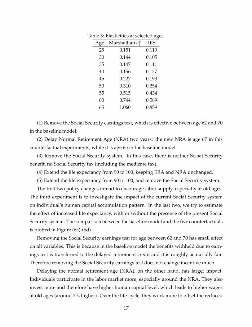
Table 3: Elasticities at selected ages.Age Marshallian εu

t IES25 0.151 0.11930 0.144 0.10535 0.147 0.11140 0.156 0.12745 0.227 0.19350 0.310 0.25455 0.515 0.43460 0.744 0.58965 1.060 0.859

(1) Remove the Social Security earnings test, which is effective between age 62 and 70

in the baseline model.

(2) Delay Normal Retirement Age (NRA) two years: the new NRA is age 67 in this

counterfactual experiments, while it is age 65 in the baseline model.

(3) Remove the Social Security system. In this case, there is neither Social Security

benefit, no Social Security tax (including the medicare tax).

(4) Extend the life expectancy from 90 to 100, keeping ERA and NRA unchanged.

(5) Extend the life expectancy from 90 to 100, and remove the Social Security system.

The first two policy changes intend to encourage labor supply, especially at old ages.

The third experiment is to investigate the impact of the current Social Security system

on individual’s human capital accumulation pattern. In the last two, we try to estimate

the effect of increased life expectancy, with or without the presence of the present Social

Security system. The comparison between the baseline model and the five counterfactuals

is plotted in Figure (6a)-(6d).

Removing the Social Security earnings test for age between 62 and 70 has small effect

on all variables. This is because in the baseline model the benefits withheld due to earn-

ings test is transferred to the delayed retirement credit and it is roughly actuarially fair.

Therefore removing the Social Security earnings test does not change incentive much.

Delaying the normal retirement age (NRA), on the other hand, has larger impact.

Individuals participate in the labor market more, especially around the NRA. They also

invest more and therefore have higher human capital level, which leads to higher wages

at old ages (around 2% higher). Over the life-cycle, they work more to offset the reduced

17

Social Security benefit, and this response happens before and after the effective NRA.

Removing the entire Social Security benefits and taxes induce higher LFPR, especially

at old ages. The investment and human capital level for an average individual is also

higher at all ages in this experiment. This indicates that the presence of the Social Security

system has some level of distortion—it increases the incentive to work at young ages

disproportionally.

The distortion effect partly explains that in the fourth experiment where each worker

lives ten extra years. In this case, each individual supplies more labor while young but

enjoys more leisure after 40s. The average LFPR and human capital level over the life-

cycle are actually lower when the life span is larger.

As comparison, the fifth experiment removes the Social Security system when each

individual lives ten extra years. Comparing with the third experiment (No SS), the LFPR,

investment and human capital level, and wages, are universally higher at all ages when

the life span is larger, in the absence of the Social Security system. This implies that

the current Social Security system has negative effect on growth in the context of im-

proved mortality and increased life-expectancy, which most countries are experiencing.

Even though the current U.S. Social Security system is largely a Pay-As-You-Go program,

Echevarría and Iza (2006) have similar findings for a funded Social Security system.

Another point worth noticing is that, in all five experiments, the responses in the

endogenously determined wages are non-trivial, especially at old ages: −4% in extending

life expectancy by ten years, −2% when removing earnings test, 2% if delaying NRA

by two years, and over 20% when removing Social Security system. For this reason, it

is likely that ignoring human capital investment channel will generate bias in terms of

predicting LFPR at old ages in similar experiments.

8. Concluding Remarks

This paper develops and estimates a Ben-Porath human capital model with endogenous

labor supply and retirement, combining the standard Ben-Porath human capital model

with the standard retirement model. In the model each individual makes decisions on

consumption, human capital investment, labor supply and retirement. The investment in

the human capital generates the wage growth over the life-cycle, while the depreciation

of the human capital is the main driving force for retirement. We show that the simple

18

model is able to fit the main features of lifecycle labor supply and wages. Given that this

is still work in progress, it is premature for conclusions beyond this.

19

References

Ben-Porath, Yoram, “The Production of Human Capital and the Life Cycle of Earnings,”

Journal of Political Economy, August 1967, 75 (4), 352–365.

Blau, David M., “Retirement and Consumption in a Life Cycle Model,” Journal of Labor

Economics, January 2008, 26 (1), 35–71.

Browning, M., L. Hansen, and J. Heckman, “Micro Data and General Equilibrium Mod-

els,” Handbook of Macro Economics, 1999, 1, 525–602.

Casanova, Maria, “Happy Together: A Structural Model of Couples’ Joint Retirement

Choices,” November 2010. Working paper.

, “Revisiting the Hump-Shaped Wage Profile,” August 2013. Working paper.

DeNardi, Mariacristina, “Wealth Inequality and Intergenerational Links,” The Review of

Economic Studies, July 2004, 71 (3), 743–768.

Echevarría, Cruz A and Amaia Iza, “Life expectancy, human capital, social security and

growth,” Journal of Public Economics, 2006, 90 (12), 2323–2349.

French, Eric, “The Effects of Health, Wealth and Wages on Labor Supply and Retirement

Behavior,” Review of Economic Studies, April 2005, 72 (2), 395–427.

and John Bailey Jones, “The effects of Health Insurance and Self-Insurance on Retire-

ment Behavior,” Econometrica, May 2011, 79 (3), 693–732.

Gustman, Alan L. and Thomas L. Steinmeier, “A Structural Retirement Model,” Econo-

metrica, May 1986, 54 (3), 555–584.

and , “Social Security and Retirement Dynamics,” July 2006. Final Report, Michigan

Retirement Research Center, UM05-05.

and , “How Changes in Social Security Affect Recent Retirement Trends,” Research

on Aging, March 2009, 31 (2), 261–290.

Haan, Peter and Victoria Prowse, “Longevity, Life-cycle Behavior and Pension Reform,”

June 2012. Working paper.

20

Haley, W., “Estimation of the Earnings Profile from Optimal Human Capital Accumula-

tion,” Econometrica, 1976, 44 (6), 1223–1288.

Heckman, James J., “A Life-Cycle Model of Earnings, Learning, and Consumption,” The

Journal of Political Economy, August 1976, 84 (4), S11–S44.

, Lance Lochner, and Christopher Taber, “Explaining Rising Wage Inequality: Expla-

nations With A Dynamic General Equilibrium Model of Labor Earnings With Hetero-

geneous Agents,” Review of Economic Dynamics, 1998, 1 (1), 1–58.

Heckman, J.J., L. Lochner, and P. Todd, “Earnings Functions, Rates of Return, and Treat-

ment Effects: The Mincer Equation and Beyond,” in E. Hanushek and F. Welch, eds.,

Handbook of the Economics of Education, Vol. 1 Elsevier Science 2006.

Hubbard, R. Glenn, Jonathan Skinner, and Stephen P. Zeldes, “Precautionary Saving

and Social Insurance,” The Journal of Political Economy, April 1995, 103 (2), 360–399.

Imai, Susumu and Michael P. Keane, “Intertemporal Labor Supply and Human Capital

Accumlation,” International Economic Review, May 2004, 45 (2), 601–641.

Johnson, Richard W and David Neumark, “Wage declines among older men,” The Re-

view of Economics and Statistics, 1996, pp. 740–748.

Keane, Michael P. and Kenneth I. Wolpin, “The Career Decisions of Young Men,” Journal

of Political Economy, June 1997, 105 (3), 473–522.

Kuruscu, B., “Training and Lifetime Income,” American Economic Review, June 2006, 96

(3), 832–846.

Madrian, Brigitte C and Lars John Lefgren, “An approach to longitudinally matching

Current Population Survey (CPS) respondents,” Journal of Economic and Social Measure-

ment, 2000, 26 (1), 31–62.

Manuelli, Rodolfo E., Ananth Seshadri, and Yongseok Shin, “Lifetime Labor Supply

and Human Capital Investment,” January 2012. Working paper.

Mincer, Jacob, “Investment in Human Capital and Personal Income Distribution,” Journal

of Political Economy, August 1958, 66 (4), 281–302.

21

Prescott, Edward C., Richard Rogerson, and Johanna Wallenius, “Lifetime aggregate

labor supply with endogenous workweek length,” Review of Economic Dynamics, 2009,

12, 23–36.

Rogerson, Richard and Johanna Wallenius, “Fixed Costs, Retirement and the Elasticity

of Labor Supply,” October 2010. mimeo, Arizona State University.

Rosen, S., “A Theory of Life Earnings,” Journal of Political Economy, 1976, 84 (4), S45–S67.

Rupert, Peter and Giulio Zanella, “Revisiting wage, earnings, and hours profiles,” June

2012. Working paper.

Rust, John and Christopher Phelan, “How Social Security and Medicare Affect Retire-

ment Behavior In a World of Incomplete Markets,” Econometrica, July 1997, 65 (4), 781–

831.

Shaw, Kathryn L., “Life-Cycle Labor Supply with Human Capital Accumulation,” Inter-

national Economic Review, May 1989, 30 (2), 431–456.

Taber, Christopher, “Tax Reform and Human Capital Accumulation: Evidence from an

Empirical General Equilibrium Model of Skill Formation,” Advances in Economic Analy-

sis and Policy, 2002, 2 (1).

Wallenius, Johanna, “Human Capital Accumulation and the Intertemporal Elasticity of

Substitution of Labor,” September 2009. Working paper.

Weiss, Yoram, “The determination of lifecycle earnings: A survey,” in Orley Ashenfelter

and David Card, eds., Handbook of Labor Economics, Vol. 1, Amsterdam: North-Holland,

1986, pp. 603–640.

22

Figure 1a: Labor Force Participation Rate-SIPP Data.2

.4.6

.81

La

bo

r fo

rce

pa

rtic

ipa

tio

n r

ate

s

22 30 40 50 60 65Age

Figure 1b: Difference of LFPR between good health and bad health-HRSData

0.0

5.1

.15

.2D

iffe

ren

ce

in

LF

PR

20 40 60 80Age

Data

Smoothed

23

Figure 1c: Log Wages-SIPP Data2

.22

.42

.62

.8O

bse

rve

d w

ag

es

22 30 40 50 60 65Age

lnw

lnw (FE)

Figure 2d: Log wage profiles, CPS MORG and March, high school grad-uates

22

.22

.42

.62

.83

lnw

18 20 30 40 50 60 65Age

MORG, lnw

March, lnw

MORG, lnw (FE)

March, lnw (FE)

24

Figure 3a: Fit of Model: Labor Force Participation Rate.2

.4.6

.81

lfp

r

22 30 40 50 62 65Age

Simulation

Data

Figure 3b: Fit of Model: Log Wages after controlling for individual fixedeffects

2.2

2.3

2.4

2.5

2.6

2.7

lnw

_fe

22 30 40 50 62 65Age

Simulation

Data

25

Figure 3c: Fit of Model: Log Wages2

.22

.42

.62

.8ln

w

22 30 40 50 62 65Age

Simulation

Data

Figure 3d: Fit of Model: Difference of LFPR between workers with goodhealth and bad health

.04

.06

.08

.1lfp

r_d

iff

22 30 40 50 62 65Age

Simulation

Data

26

Figure 4a: log wages, with and without controlling for individual fixedeffects

2.2

2.3

2.4

2.5

2.6

2.7

Sim

ula

ted

wa

ge

pro

file

s

22 30 40 50 62 65t

lnw

lnw_fe

Figure 4b: Labor supply, log wages, and income

05

10

15

Inco

me

0.2

.4.6

.81

LF

PR

22

.22

.42

.62

.8ln

w

22 30 40 50 6265 70 80 90Age

lnw

lnw (FE)

LFPR

Income

27

Figure 4c: Leisure, investment, and human capital

05

10

15

20

Hu

ma

n C

ap

ita

l

0.2

.4.6

.81

22 30 40 50 62 65 70 80 90Age

Leisure Investment Human Capital

Figure 4d: log wages and human capital

05

10

15

20

Hu

ma

n C

ap

ita

l

22

.22

.42

.62

.8

22 30 40 50 62 65 70 80 90Age

lnw

lnw (FE)

Human Capital

28

Figure 5a: Calculated elasticities0

.2.4

.6.8

1E

lasticitie

s

20 30 40 50 60 70Age

Marshallian

IES

Figure 5b: LFPR profiles for positive shocks at different ages

0.2

.4.6

.81

lfp

r

20 40 60 80 100Age

Baseline

Shock at 25

Shock at 40

Shock at 60

29

Figure 5c: Total changes in LFPR for positive shocks at different ages−

.3−

.2−

.10

.1lfp

r

20 30 40 50 60 70Shock age

Overall

Before t

After t

At t

Figure 6a: Counterfactual experiments: difference in LFPR

−.0

50

.05

.1.1

5.2

d_

lfp

r

20 30 40 50 60 70 80 90 100Age

No ET

NRA=67

No SS

LE+10

LE+10, No SS

30

Figure 6b: Counterfactual experiments: difference in lnw−

.10

.1.2

.3d

_ln

w

20 30 40 50 60 70 80 90 100Age

No ET

NRA=67

No SS

LE+10

LE+10, No SS

Figure 6c: Counterfactual experiments: difference in human capital lev-els

−1

01

23

4d

_H

20 30 40 50 60 70 80 90 100Age

No ET

NRA=67

No SS

LE+10

LE+10, No SS

31

Figure 6d: Counterfactual experiments: difference in investment−

.02

0.0

2.0

4.0

6.0

8d

_I

20 30 40 50 60 70 80 90 100Age

No ET

NRA=67

No SS

LE+10

LE+10, No SS

32