A hybrid indirect boundary element—discrete wave number method

applied to simulate the seismic response of stratified alluvial valleys

S.A. Gil-Zepeda, J.C. Montalvo-Arrieta, R. Vai, F.J. Sanchez-Sesma*

Instituto de Ingenierıa, UNAM, Ciudad Universitaria, Apdo. 70-472, Coyoacan, 04510 Mexico, DF, Mexico

Accepted 13 July 2002

Abstract

A hybrid indirect boundary element – discrete wavenumber method is presented and applied to model the ground motion on stratified

alluvial valleys under incident plane SH waves from an elastic half-space. The method is based on the single-layer integral representation for

diffracted waves. Refracted waves in the horizontally stratified region can be expressed as a linear superposition of solutions for a set of discrete

wavenumbers. These solutions are obtained in terms of the Thomson–Haskell propagators formalism. Boundary conditions of continuity of

displacements and tractions along the common boundary between the half-space and the stratified region lead to a system of equations for the

sources strengths and the coefficients of the plane wave expansion. Although the regions share the boundary, the discretization schemes are

different for both sides: for the exterior region, it is based on the numerical and analytical integration of exact Green’s functions for

displacements and tractions whereas for the layered part, a collocation approach is used. In order to validate this approach results are compared

for well-known cases studied in the literature. A homogeneous trapezoidal valley and a parabolic stratified valley were studied and excellent

agreement with previous computations was found. An example is given for a stratified inclusion model of an alluvial deposit with an irregular

interface with the half-space. Results are displayed in both frequency and time domains. These results show the significant influence of lateral

heterogeneity and the emergence of locally generated surface waves in the seismic response of alluvial valleys.

q 2002 Elsevier Science Ltd. All rights reserved.

Keywords: Collocation; Diffraction; Earthquakes; Elastodynamics; Green’s functions; Indirect boundary element method; Locally generated surface waves;

Seismic ground motion; Seismic response; Site effects; Synthetic seismograms; Stratified alluvial valley; Thomson–Haskell propagators

1. Introduction

Local geological conditions may generate significant

amplification of ground motion and concentrated damage

during earthquakes. There are important advances in the

evaluation of such effects [1–3]. In most situations local

amplification can be inferred reasonably using simple one-

dimensional (1D) shear models. However, lateral hetero-

geneity may give rise to focusing and to locally generated

surface waves; therefore, the estimates for local amplifica-

tion using 1D models may be wrong. Although the physics

of this phenomenon is now reasonably well understood,

most of the rigorous procedures require large amounts of

computer resources. We believe there is a lack of practical

methods for the assessment of local amplification.

Boundary element methods (BEM) have gained increas-

ing popularity. Recognized advantages over domain

approaches are the dimensionality reduction, the relatively

easy fulfillment of radiation conditions at infinity and the

high accuracy of results. Excellent surveys of the available

literature on BEM in elastodynamics are by Manolis and

Beskos [4]; Beskos [5,6]. One useful approach is the indirect

boundary element method (IBEM), which formulates the

problem in terms of force densities at the boundaries [7–9].

On the other hand, in their pioneering work, Aki and

Larner [10] introduced a numerical method based on a

discrete superposition of homogenous and inhomogeneous

plane waves. Using this technique, Bard and Bouchon [11,

12] studied alluvial valleys and pointed out the significant

role of basin-induced surface waves in the valley’s response

and studied the resonant characteristics of these

configurations as well. The Aki–Larner’s technique is the

departure of discrete wavenumber approximations.

The combination of discrete wavenumber expansions for

Green’s functions with boundary integral representations

has been successful in various studies of elastic wave

propagation [13–15].

0267-7261/03/$ - see front matter q 2002 Elsevier Science Ltd. All rights reserved.

PII: S0 26 7 -7 26 1 (0 2) 00 0 92 -1

Soil Dynamics and Earthquake Engineering 23 (2003) 77–86

www.elsevier.com/locate/soildyn

* Corresponding author.

E-mail address: sesma@servidor.unam.mx (F.J. Sanchez-Sesma).

The combination of a BEM-type approach with a discrete

wavenumber formulation to compute the Green’s function

is particularly attractive: the singularities of Green’s

functions are not present in each one of the terms of the

discrete wavenumber expansion [14,16]. The integration

along the boundary effectively makes the singularities to

vanish and improves convergence as well. However, such

procedures require considerable amount of computer

resources. An alternative that may be welcomed for some

applications could be the IBEM, with analytical Green’s

functions for the half-space, and a discrete wavenumber

expansion for the layered part. A similar idea, that uses line

sources close to the boundary, propagators for the layered

part and the least-squares method, was proposed by Bravo

et al. [17].

In this work we extend the Bravo et al. [17] approach by

placing the sources at the very boundary [7] so that the

singularities of the sources are dealt with analytically.

Therefore, the IBEM is applied for the half-space. The

sources strengths and the coefficients for the discrete

wavenumber expansion equal in number the conditions

(continuity of displacements and tractions) at the colloca-

tion points in the interface.

2. Formulation of the problem

Consider a horizontally stratified deposit in a hom-

ogenous half-space. Elastic materials occupy the entire

domain. With reference to Fig. 1, we designate by S the

boundary between the region R, which is the stratified

medium, and the exterior domain E. In Fig. 1 we show also

the cross-section of the stratified model and the harmonic

incident SH wave. In order to compute the displacement

field at the free surface, we treat the two regions separately.

Continuity of displacement and traction at S will then be

imposed.

2.1. Domain E

As far as the domain E is concerned, the ground motion

comes from the interferences of incoming waves with

reflected and diffracted ones. The total motion in the half-

space is the superposition of the free-field and the so called

diffracted waves:

vE ¼ vð0Þ þ vðdÞ; ð1Þ

where v (0) is the free field displacement, i.e. the solution in

the absence of the irregularity. The free-field displacement

at a point x ¼ ðx; zÞ is

vð0ÞðxÞ ¼ e2iðkx2hzÞ þ e2iðkxþhzÞ; ð2Þ

where k ¼ ðv=bÞsin g and h ¼ ðv=bÞcos g are the horizontal

and vertical wavenumbers, respectively, v is the angular

frequency, b the shear waves velocity in the domain E, g the

incidence angle. We are dealing with antiplane SH waves,

i.e. all of the displacement are perpendicular to the x–z

plane.

Let us discretize the surface S by N straight segments of

longitude DS and call jl ¼ ðx1; z1Þ the midpoint of the

segment l. Neglecting body forces, the diffracted field can

be written as

vðdÞðxÞ ¼XNl¼1

fðjlÞgðx; jlÞ; ð3Þ

where f(jl) is the unknown force density assumed to be

constant (fl) along the corresponding DS;

gðx; jÞ ¼ðDSl

Gðx; jÞdSj; ð4Þ

where G(x,j ) is the Green’s function of a line source in a

half-space, i.e. the displacement at point x due to the

application of two unit forces at point j ¼ ðxl; zlÞ and at its

image j0 ¼ ðxl 2 zlÞ: Therefore, one has

Gðx; jÞ ¼1

i4mHð2Þ

0 rl

v

b

� �þ Hð2Þ

0 r0lv

b

� �� �; ð5Þ

where Hð2Þ0 ð·Þ is Hankel’s function of the second kind and

zero order, rl and r0l are the distances between the point x and

the sources jl and its image j0l; respectively. The use of an

image source guarantees that the boundary conditions of

null tractions at the half-space free surface are automatically

satisfied in Eq. (3).

The integral in Eq. (4) is performed on the variable j;

Gaussian integration is used. G(x,j ) presents a logarithmic

integrable singularity at x ¼ j; where x is in the neighbor-

hood of j, the second right term of Eq. (5) is treated

numerically, while for the first one we obtained the analytical

expressions from the ascending series for Hankel’s functions

[18]. Sanchez-Sesma and Campillo [7] presented an example

for such expressions where only the leading terms of the

series are retained. We considered up to quadratic terms,

which is enough if the number of segments per wavelength is

larger than about five.

The quantities fðjlÞDS represent a force distribution at

the boundary. Eq. (3) is simply the discretized form of a

single layer integral, that can be obtained from Somigliana

identity [7], and has been studied by Kupradze [19] from

the point of view of potential theory. He showed that

Fig. 1. Half-space, E, with a horizontally stratified alluvial valley, R. The

incidence of SH waves with angle g is depicted. The only discretization

needed is along the interface S. In the free surface of the layered part and the

flat surface of the half-space the boundary conditions are satisfied by

construction.

S.A. Gil-Zepeda et al. / Soil Dynamics and Earthquake Engineering 23 (2003) 77–8678

the displacement field (3) continuous across S if f(j ) is

continuous along S. The scalar 2D version that we are using

is also called the Kirchhoff–Helmhotz representation [20].

Likewise the displacement field, we express the tractions

in the half-space as the superposition of the contributions

from the free-field and the diffracted one:

tE ¼ tð0Þ þ tðdÞ: ð6Þ

Since we are dealing with an antiplane problem the traction

vector can be represented by a scalar quantity, when a vector

n lying in the plane is specified. In fact, applying Hooke’s

law we have:

tE ¼ m›v

›n; ð7Þ

where n is assumed to be specified. Developing Eq. (7) we

find Cauchy’s equation:

tE ¼ m›v

›n¼ m

›v

›x

›x

›nþ

›v

›z

›z

›n

� �

¼ m›v

›xnx þ

›v

›znz

� �¼ syxnx þ syznz: ð8Þ

Therefore, the free-field traction is expressed by:

tð0ÞðxÞ ¼ ½2iknx þ ihnz�e2iðkx2hzÞ 2 ½iknx þ ihnz�e

2iðkxþhzÞ;

ð9Þwhich clearly displays in the two groups of terms:

the incident and reflected waves, respectively. In analogous

terms the diffracted tractions can be computed by means of:

tðdÞðxÞ ¼XNl¼1

fðjlÞtðx; jlÞ; ð10Þ

where t (d )(x) is the traction at point x, fðjlÞ ¼ fl; tðx; jÞ is

given by:

tðx;jÞ ¼ð

STðx; jÞdSj; ð11Þ

where T(x,j ) is the traction Green’s function, i.e. the

traction at point x on the boundary S with normal n(x)

(assumed to be specified and pointing outside E) due to the

application of two unit forces at point j and at its image j0.

Its formal expression is

Tðx; jlÞ ¼iv4b

›rl

›nHð2Þ

l rl

v

b

� �þ

›r0l›n

Hð2Þl r0l

v

b

� �� �; ð12Þ

where Hð2Þl ð·Þ is the Hankel’s function of the second kind

and first order. The integral in Eq. (11) is also computed

numerically using Gaussian integration. The traction

Green’s function presents a singularity of the form 1/r

when xj ¼ jl; in this case we obtain

tðxj; jlÞ ¼ 0:5djl þðDSl

iv

4b

›r0l›n

Hð2Þl r0l

v

b

� �� �dSj 0

j ¼ l:

ð13Þ

djl is the Kronecker symbol ( ¼ 1 if j ¼ l, ¼ 0 if j – l).

The formal contribution from the source j to the integral is

null because the discretization segment is a straight line

and jl is the midpoint. In fact, it can be verified that, under

this circumstance, such part of the integrand is a singular

odd function on the segment. Therefore, its Cauchy’s

principal value is zero. The contribution of singularity has

been already taken into account in the first term of Eqs.

(11) and (13). This result has also been found by Kupradze

[19]. In its scalar version, the result appeared first in a

paper by Fredholm in 1900 [21].

2.2. Domain R

The ground motion in the region R is generated by waves

refracted at S and at the interfaces of the layers. For the

solution in the stratified medium, we combine Thomson–

Haskell’s propagator matrices ([22,23]) in the framework of

a discrete wavenumber representation. In this way, the

refracted field in the region R can be written as:

vðrÞðxÞ ¼XM

m¼2M

Bml1ðkm; z;vÞe2ikmx

; ð14Þ

where Bm are the unknown complex coefficients and

l1ðkm; z;vÞ is the first element of the motion-stress vector

for Love waves [24] for the horizontal discrete wavenumber

km. The function l1ðkm; z;vÞe2ikmx is solution of the 2D

Helmholtz equation within the layered system. If, for

example, we make

vðxÞ ¼ l1ðk; z;vÞe2ikx ð15Þ

and define the traction at horizontal planes as:

m›v

›z¼ l2ðk; z;vÞe

2ikx; ð16Þ

where l1 and l2 are continuous functions of z. Then it can be

shown Ref. [24] that, in a medium composed of horizontal

homogeneous layers, the motion-stress vector at depth z can

be written in terms of the propagator matrix and the motion-

stress vector at depth z0 as

l1

l2

" #z

¼ Pðz; z0Þl1

l2

" #z0

: ð17Þ

The propagator matrix for a homogeneous medium is given

by

Pðz; z0Þ ¼cos hðz2 z0Þ ðhmÞ21 sin hjðz2 z0Þ

2hm sin hjðz2 z0Þ cos hðz2 z0Þ

24

35;ð18Þ

where h¼ffiffiffiffiffiffiffiffiffiffiffiffiffiffiv2=b2 2 k2

p:

S.A. Gil-Zepeda et al. / Soil Dynamics and Earthquake Engineering 23 (2003) 77–86 79

From the repeated application of Eq. (17), if we assume

that z0 ¼ 0 corresponds to the free surface, we have

Pðz; z0Þ ¼ Pðz; zj21ÞPðzj21; zj22Þ…Pðz1; z0Þ; ð19Þ

for zj $ z $ zj21 that is, for z in the jth stratum. The form of

Eq. (19) guarantees satisfaction of continuity of stress and

displacement between adjacent layers. To satisfy the

boundary condition at the free surface, we make l2 ¼ 0 at

z ¼ 0:Without loss of generality, we can choose l1 ¼ 1 at the

free surface.

The displacement is directly related to the first

component of the motion-stress vector (see Eq. (15)),

while the traction associated to a vector n ¼ ðnx; nzÞT;

considering Eqs. (15) and (16), can be expressed as

t ¼m›v

›n¼m

›v

›xnx þ

›v

›znz

� �¼2imkl1nx e2ikx þ l2nz e2ikx

:

ð20Þ

2.3. Coupling regions E and R

To guarantee perfect bonding between regions E and

R we impose continuity of displacement and tractions,

i.e.

vðrÞ ¼ vð0Þ þ vðdÞ ð21Þ

at S, and

tðrÞ ¼ tð0Þ þ tðdÞ ð22Þ

at S.

These conditions can be expressed for a point x on (the

common interface) S by means of

XNl¼1

flgðx; jlÞ2XM

m¼2M

Bmllðkm; z;vÞe2ikmx ¼ 2vð0ÞðxÞ; ð23Þ

and

XNl¼1

fltðx; jlÞ þXM

m¼2M

Bmð2imnxllðkm; z;vÞ

þ nzl2ðkm; z;vÞÞe2ikmx ¼ 2tð0ÞðxÞ; ð24Þ

respectively. If we impose these conditions on a set of points

along the boundary S we can speak of a collocation scheme.

Assume we chose x ¼ ðxj; zjÞ; j ¼ 1;…;N; evenly distrib-

uted S. Then in order to obtain a square system of equation

we set N ¼ 2M þ 1: It becomes clear that the total number

of equations is 2N which is the same as the number of

unknowns.

The choice of N is guided by the following consider-

ations. In the region E it is convenient to have at least five

elements per wavelength. This criterion comes from

previous experiences using IBEM [7] and it is somewhat

conservative. For shallow valleys one can approximately

obtain N . 5h, where h ¼ ðvaÞ=ðpbEÞ is the normalized

frequency and a the half-width of the valley. If the

sediments were to be treated with IBEM too, then an

estimate of the lower bound for N in the layered region

could be N . 5hðbE=bminÞ; which, for valleys with very soft

layers may produce very large N and this gives unnecess-

arily dense sampling for both the half-space and the valley.

This statement is clear of one considers the global nature of

the discrete wavenumber expansion which is given in terms

of eikmx: Moreover, it is convenient to assume that Dk is

less than p/a, to avoid spurious periodicities, and that

only homogeneous waves are allowed in the softer layer

(this means kmax ¼ v=bmin and implies that inhomo-

geneous waves can exist in the other layers). Then, we

have M . hðbE=bminÞ; which gives N . 2hðbE=bminÞ þ 1:

Obviously, this value is less restrictive but still it can very

easily dominate the choice of N. If the amount of allowed

inhomogeneous waves in the softer layer is increased (this

means kmax . v=bminÞ; N becomes larger.

For low frequencies, oversampling is not a serious

problem. Actually, it is convenient and the solution is very

stable. When frequency increases the different character of

the involved representations requires care. A moderate

amount of inhomogeneous waves may give good results for

intermediate frequencies. Sometimes undersampling is a

good solution. However, all this requires further scrutiny.

The formulation for the P–SV waves case, would be part of

another research.

3. Testing of the method

The accuracy of our approach is tested here using a

solution that has been verified extensively [14]. These

authors used direct boundary elements with the Green’s

function computed using the discrete wavenumber

method. Their results have been tested by Ramos-

Martinez [25] and Zahradnik [26], among others. There-

fore, we regard these results as trustworthy.

Kawase and Aki [14] studied the trapezoidal valley shown

in Fig. 2. Comparisons with their results are provided here for

vertical incidence of plane SH waves. The model response is

Fig. 2. Model studied by Kawase and Aki [14]. The regions E and R are

shown and the coordinates are normalized in terms of the half-width

a ¼ 5 km. Incidence of harmonic SH waves. Material properties are given

in the text.

S.A. Gil-Zepeda et al. / Soil Dynamics and Earthquake Engineering 23 (2003) 77–8680

computed in frequency domain and the synthetic seismo-

grams are computed using the FFT algorithm. It was assumed

an incident Ricker wavelet. The comparison in time domain

is a good test as many frequencies have to be computed and

synthesized to provide the results. The synthetic seismo-

grams obtained from both methods for vertical incidence are

shown in Figs. 3 and 4 for characteristic periods tp ¼ 4 and

2 s, respectively. The agreement is excellent. We computed

also the synthetics for an incidence angle of 308 with respect

to the vertical and Fig. 5 shows the seismograms at the free

Fig. 3. Synthetic seismograms at the surface of Kawase and Aki’s model

[14] for vertical incidence of plane SH waves with time variation given by a

Ricker pulse with characteristic period of 4 s. (a) Kawase and Aki [12] and

(b) the presented approach.

Fig. 4. Same as Fig. 3 but with characteristic period of 2 s.

Fig. 5. Synthetic seismograms at the surface of Kawase and Aki’s model

[14], computed with the presented approach, for oblique incidence ðg ¼

308Þ of plane SH waves with time variation given by a Ricker pulse with

characteristic period of (a) 4 and (b) 2 s.

Fig. 6. Model studied by Bravo et al. [17]. Ratios of velocities of S waves

and mass densities considered are: b1=bE ¼ 1=3; b1=bE ¼ 2=3 and r1=rE ¼

3=4; r2=rE ¼ 0:85:

S.A. Gil-Zepeda et al. / Soil Dynamics and Earthquake Engineering 23 (2003) 77–86 81

surface for characteristic periods tp ¼ 4 and 2 s, respectively.

These results clearly display the great significance of locally

generated surface waves at the valley’s edges.

We compared our approach also with the results by

Bravo et al. [17]. These authors studied the response of a

stratified parabolic deposit depicted in Fig. 6. Region R

consists of two homogeneous strata, the top layer being 1.

Maximum thickness are H1 ¼ a=6 and H2 ¼ a=3; where a is

the half-width of the deposit. Shear-wave velocities and

mass densities, referred to those of the half-space, are

b1=bE ¼ 1=3; b1=bE ¼ 2=3 and r1=rE ¼ 3=4; r2=rE ¼ 0:85:

Figs. 7 and 8 show the comparisons with their results.

Three angles of incidence g ¼ 0; 30 and 608 were

considered, and two normalized frequencies h ¼ 1:0 and

2.0, respectively. The agreement is excellent.

4. Example

4.1. A layered soft deposit

In order to illustrate a complete set of results we analyze

the response of a stratified valley with irregular interface for

three incident angles in both frequency and time domains.

The model is shown in Fig. 9. The half-width is of 1 km and

Fig. 8. Same as Fig. 7 but for a normalized frequency of h ¼ 1:0: Fig. 11. Displacement amplitude at surface receivers at the layered valley

along the x-axis for three incidences. Normalized frequency h ¼ 1:0:

Fig. 12. Displacement amplitude at surface receivers at the layered valley

along the x-axis for three incidences. Normalized frequency h ¼ 1:5:

Fig. 7. Comparison of displacement amplitudes on the surface of the

parabolic stratified deposit of Fig. 6. Normalized frequency is h ¼ 1:0 and

incident angles are g ¼ 0; 30 and 608. Lines are for Bravo et al., and

symbols are our approach.

Fig. 9. Model of a layered valley. The coordinates are normalized in terms

of the half-width a ¼ 1 km. Incidence of harmonic SH waves. Material

properties are given in the text.

Fig. 10. Displacement amplitude at surface receivers at the layered valley

along the x-axis for three incidences. Normalized frequency h ¼ 0:8:

S.A. Gil-Zepeda et al. / Soil Dynamics and Earthquake Engineering 23 (2003) 77–8682

maximum depth is 0.35 km. The shear wave velocity

assumed for the half-space is b ¼ 2 km=s; while the

velocities of the four layers, from top to bottom, are 0.8,

0.6, 1.0 and 1.2 km/s, the corresponding thicknesses of the

four layers are 50, 100, 100 and 100 m, respectively, and the

quality factor used are 50, 100, 150 and 200, respectively.

Three angles of incidence g ¼ 0; 30 and 2308 were

considered. Figs. 10–12 shows the surface displacement

amplitudes for normalized frequencies h ¼ 0:8; 1.0 and 1.5,

respectively. Because of the properties of the model these

frequencies have the same numerical value in Hz. The various

plots clearly illustrate the spatial variation of amplification

and the effect of incidence angle.

In order to give a clearer idea of the response,

Figs. 13–15 show the contours of displacement amplitudes

at surface receivers along the x-axis, between x ¼ 20:94

Fig. 13. Contours of displacement amplitude for surface receivers along the x-axis against frequency. Layered valley under vertical incidence of SH waves.

Fig. 14. Contours of displacement amplitude for surface receivers along the x-axis against frequency. Layered valley under oblique incidence ðg ¼ 308Þ of SH

waves.

S.A. Gil-Zepeda et al. / Soil Dynamics and Earthquake Engineering 23 (2003) 77–86 83

km and x ¼ 0:94 km; against normalized frequency. These

f–x diagrams display the transfer function (relative to

the amplitude of incident waves) for all receivers and

provide a good description of the frequency behavior of

the valley. The plots also evince lateral resonances, which

sometimes are clear when a series of peaks are distributed in

space for a given frequency. This effect has been identified

before [8]. The layering and the irregular profile tend to

produce a complicated response. The resonant patterns vary

with incidence angle. For instance, a resonant frequency of

about 2.7 is clear for vertical incidence, but such a

frequency is little excited by the oblique incidences.

The maximum value of displacement amplitudes is

of about 12 for a frequency of about 1 Hz. This

amplification, relative to the horizontal free-field surface

displacement, is of about 6.5, nearly three times the average

impedance ratio. On the other hand, the frequency is almost

two times the 1D shear resonant frequency for a flat layer of

the left side of the valley depth of 200 m). The same effects

can be seen at the right side and can well be explained in

terms increased stiffness due to lateral confinement. The 1D

model gives surface amplitudes of about 4. Thus, we are led

to interpret that the large amplification is associated to the

lateral effects. These in turn, are due to focusing and to

locally generated surface waves.

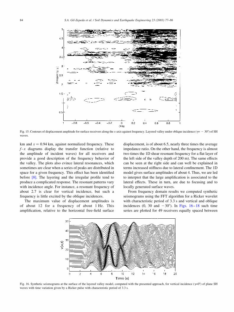
From frequency domain results we computed synthetic

seismograms using the FFT algorithm for a Ricker wavelet

with characteristic period of 3.3 s and vertical and oblique

incidences (0, 30 and 2308). In Figs. 16–18 such time

series are plotted for 49 receivers equally spaced between

Fig. 15. Contours of displacement amplitude for surface receivers along the x-axis against frequency. Layered valley under oblique incidence (g= 2 308) of SH

waves.

Fig. 16. Synthetic seismograms at the surface of the layered valley model, computed with the presented approach, for vertical incidence (g=08) of plane SH

waves with time variation given by a Ricker pulse with characteristic period of 3.3 s.

S.A. Gil-Zepeda et al. / Soil Dynamics and Earthquake Engineering 23 (2003) 77–8684

x ¼ 20:94 km and x ¼ 0:94 km: The amplification effect

seen in the frequency domain is also clear in the synthetics.

The traces show some ‘ringing’ which is probably due to

errors in the computation of transfer functions and/or to the

fact that we interpolated frequency response to obtain the

synthetics.

5. Conclusions

A hybrid indirect boundary element-discrete

wavenumber method has been presented and applied to

study the seismic response of horizontally stratified alluvial

valleys of arbitrary shape for incidence of plane SH waves.

The method is based upon the integral representation of

scattered and diffracted elastic waves at the half-space in

terms of single layer boundary sources. For this IBEM

approach, the Green’s function was selected to be the one

for the half-space and the discretization is restricted to

the contact between the regions. For the stratified region the

field is constructed using a set of solutions for homogeneous

and inhomogeneous plane waves that correspond to hori-

zontal discrete wavenumbers (DWN). These solutions

satisfy all the boundary conditions at the layers interfaces

and are obtained in terms of Thomson–Haskell propagators

formalism.

While simple and intuitively appealing, this hybrid

approach may suffer of some drawbacks and particular

care is required from the analyst. The two approxi-

mations are different in character. On one hand, the

IBEM description is local (we seek for local physical

quantities: the force densities), on the other hand, the

DWN linear superposition is global (the needed

coefficients represent harmonic patterns). This may give

rise to large differences in the entries of the coefficient

matrix that results from the collocation scheme for

boundary conditions, thus producing large rounding

errors. By limiting the amount of allowed inhomo-

geneous wave and sampling the horizontal wavenumber

domain in such a way that spatial periodicities less than

2a are avoided we may restrict the extent of numerical

errors. This may result for some problems a kind of

undersampling. In order to fully automate this procedure

some more scrutiny is required.

Some examples are given for the response of simple

models of stratified alluvial valleys in an elastic half-space.

We confirmed the appearance of complicated patterns for

surface displacements even in simple cases. In the examples

the generation of Love surface waves can easily be seen.

Fig. 17. Same as Fig. 13 but for oblique incidence (g= 2 308).

Fig. 18. Same as Fig. 13 but for oblique incidence (g= 2 308).

S.A. Gil-Zepeda et al. / Soil Dynamics and Earthquake Engineering 23 (2003) 77–86 85

Synthetics for the irregular valley show a variety of

complex patterns. Focusing of energy at low frequencies

generally takes place at the deeper parts. Very large

amplification was found in the sediments; more than three

times the 1D prediction from the impedance contrast.

Our results suggest that variations in layer properties

may produce important effects in the response. Strong

impedance contrasts and the response at higher frequencies

are among the issues that require attention.

The method is generally fast and accurate but it is not

error-free and requires care from the analyst. Some more

work is still needed for automatical choice of the calculation

parameters.

Acknowledgements

We gratefully acknowledge the comments of two

anonymous reviewers. Thanks are given to M. Ordaz and

V.J. Palencia for their critical reviews and to

M. Mucciarelli, F. Pacor, A. Mendez, for their comments

and suggestions. This work was partially supported by

ISMES SpA of Bergamo, Italy and by DGAPA-UNAM,

Mexico, under project IN104998.

References

[1] Sanchez-Sesma FJ. Site effects on strong ground motion. Soil Dyn

Earthquake Engng 1987;6:124–32.

[2] Aki K. Local site effects on strong ground motion in earthquake

engineering and soil dynamics II. Recent advances. In: Von Thun JL,

editor. Ground motion evaluation in geotechnical special publication, vol.

20. New York: American Society of Civil Engineers; 1988. p. 103–55.

[3] Sanchez-Sesma FJ. Strong ground motion and site effects. In: Beskos

DE, Anagnostopoulos SA, editors. Computer analysis and design of

earthquake resistant structures, Southampton: Computatinal Mech-

anics Publications; 1996.

[4] Manolis GD, Beskos DE. Boundary element methods in elastody-

namics. London: Unwin Hyman Ltd; 1988.

[5] Beskos DE. Boundary element methods in dynamic analysis. Appl

Mech Rev 1987;40:1–23.

[6] Beskos DE. Boundary element methods in dynamic analysis: Part II

(1986–1996). Appl Mech Rev 1997;50:149–97.

[7] Sanchez-Sesma FJ, Campillo M. Difracction of P, SV Rayleigh waves

by topographic features: a boundary integral formulation. Bull

Seismol Soc Am 1991;81:2234–53.

[8] Sanchez-Sesma FJ, Ramos-Martınez J, Campillo M. An indirect

boundary element method applied to simulate the seismic response of

alluvial valleys for incident P, S and Rayleigh waves. Earthquake

Engng Struct Dyn 1993;22:279–95.

[9] Sanchez-Sesma FJ, Luzon F. Seismic response of three-dimensional

alluvial valleys for incident P, S and Rayleigh waves. Bull Seismol

Soc Am 1995;85:269. see also p. 284.

[10] Aki K, Larner KL. Surface motion of a layered medium having an

irregular interface due to incident plane SH waves. J Geophys Res

1970;75:1921–41.

[11] Bard P-Y, Bouchon M. The seismic response of sediment-filled

valleys. Part 1. The case of incident SH waves. Bull Seismol Soc Am

1980;70:1263–86.

[12] Bard P-Y, Bouchon M. The seismic response of sediment-filled

valleys. Part 2. The case of incident P and SV waves. Bull Seismol Soc

Am 1980;70:1921–41.

[13] Bouchon M, Campillo M, Gaffet S. A boundary integral equation—

discrete wavenumber representation method to study wave propa-

gation in multilayered media having irregular interfaces. Geophysics

1989;54:1134–40.

[14] Kawase H, Aki K. A study on the response of a soft basin for

incident. S, P and Rayleigh waves with special reference to the

long duration observed in Mexico City. Bull Seismol Soc Am

1989;79:1361–82.

[15] Papageorgiou AS, Kim J. Study of the propagation and amplifica-

tion of seismic waves in Caracas Valley with reference to the 29

July 1967 earthquake: SH waves. Bull Seismol Soc Am 1991;81:

2214–33.

[16] Kawase H. Time-domain response of a semicircular canyon for

incident SV, P, and Rayleigh waves calculated by the discrete

wavenumber boundary element method. Bull Seismol Soc Am 1988;

78:1415–37.

[17] Bravo MA, Sanchez-Sesma FJ, Chavez-Garcıa FJ. Ground motion on

stratified alluvial deposits for incident SH waves. Bull Seismol Soc

Am 1988;78:436–50.

[18] Abramowitz M, Stegun IA. Handbook of mathematical functions.

New York: Dover; 1972.

[19] Kupradze VD. Dynamical problems in elasticity. In: Sneddon IN, Hill

R, editors. Progress in solid mechanics, vol. III. Amsterdam: North

Holland; 1963.

[20] Kouoh-Bille L, Sanchez-Sesma FJ, Wirgin A. Response resonante

d’u’une montagne cylindrique a une onde sismique SH. CR Acad Sci

Paris 1991;312(II):849–54.

[21] Webster AG. Partial differential equations in mathematical physics.

New York: Dover; 1955.

[22] Thomson WT. Transmission of elastic waves through a stratified solid

medium. J Appl Phys 1950;21:89–93.

[23] Haskell NA. Dispersion of surface waves on multilayered media. Bull

Seismol Soc Am 1953;43:17–34.

[24] Aki K, Richards PG. Quantitative seismology. Theory and methods.

San Francisco: W.H. Freeman; 1980.

[25] Ramos-Martınez J. Simulacion numerica de la respuesta sismica de

valles aluviales. MSc Thesis, Institute of Geophysics, UNAM;

1992.

[26] Zahradnik J. Simple elastic finite-difference scheme. Bull Seismol Am

1995;85:1879–87.

S.A. Gil-Zepeda et al. / Soil Dynamics and Earthquake Engineering 23 (2003) 77–8686