Embed Size (px)
Citation preview

A High Throughput Low Power
Soft-Output Viterbi Decoder
By
Gan Ouyang
Supervisor: Prof. Jun Yan Ren
Examiner: Prof. Lirong, Zheng
Thesis Period: Aug 2009 — Mar 2010
Department of Microelectronics,
School of Information Science and Technology
Fudan University, Shanghai, China
Royoal Institute of Technology (KTH), Stockholm, Sweden

Acknowledgements
My deepest gratitude goes first and foremost to Professor Junyan Ren, my
supervisor, for his constant encouragement, suggestion and guidance. Second, I
would like to express my heartfelt thankfulness to Dr. Fan Ye, who led me into this
exciting research area and helped me a lot in the past three years.
I also acknowledge Professors Lirong Zheng, Shili Zhang, Hannu Tenhunen,
Axel Jantsch, Ahmed Hemani, C. M. Zetterling, Mats Brorsson, Mohammed Ismail
and Shaofang Gong for traveling thousands of miles from Sweden to Shanghai to
teach me the interesting and valuable courses that I have taken at Fudan-KTH Joint
Master Program.
I also owe my sincere gratitude to my colleagues who gave me their help and
support in the past three years. These colleagues include Xuejing Wang, Liang Liu,
Jingfeng Li, Zhuo Xu, Xiaojing Ma, Zhigui Liu, Cheng Zhang, Jun Zhou, Wenyan
Su, Xu Shen, Chenxi Li, Wei Liang, Kai Li, Yu Nie and Yunqi Zeng.
This work is in part sponsored by National Sci & Tech Major Projects of China
with grant number of 2009ZX03006-007-01. This financial support is greatly
appreciated.
At last, I would like to thank my parents for their endless love, patience,
understanding and support all through these years. This thesis is dedicated to them

I
Contents
Acknowledgements ........................................................................................................ 1
Contents ......................................................................................................................... I
List of Figures .............................................................................................................. III
List of Tables ................................................................................................................. V
摘要 .............................................................................................................................. VI
Abstract ..................................................................................................................... VIII
Chapter 1 Introduction ............................................................................................... 1
Chapter 2 The Viterbi Algorithm ............................................................................... 7
2.1 Convolutional Code and Convolutional Encoder ...................................................... 7
2.2 The Channel Mode .................................................................................................... 9
2.2.1 Discrete memoryless channel ............................................................................ 9
2.2.2 Binary Symmetric Channel ............................................................................... 9
2.2.3 Gaussian Channel ............................................................................................ 10
2.3 Maximum Likelihood Decoding ............................................................................. 10
2.3.1 Hard-Decision Decoding ................................................................................. 12
2.3.2 Soft-Decision Decoding .................................................................................. 13
2.4 The Viterbi Decoding Algorithm ............................................................................. 14
Chapter 3 The Soft Output Viterbi Algorithm ......................................................... 21
3.1 Original Formulation of SOVA ............................................................................... 21
3.2 Two-Step SOVA ...................................................................................................... 24
Chapter 4 Hardware Architecture of SOVA Decoder .............................................. 26
4.1 Convolutional Codes in the UWB Standard ............................................................ 27
4.2 Branch Metric Unit ................................................................................................. 30
4.3 Add-Compare-Select Unit ....................................................................................... 32
4.3.1 ACS VS CSA .................................................................................................. 32
4.3.2 Path Metric Normalization .............................................................................. 37
4.4 Survivor Path Management Unit ............................................................................. 39
4.4.1 The Register-Exchange Method ...................................................................... 39
4.4.2 The Trace-Back Method .................................................................................. 40
4.4.3 The Trace-Forward Method ............................................................................ 42
4.4.4 The Modified Trace-Forward Architecture ..................................................... 46
4.5 The Path Comparison Unit ...................................................................................... 50

II
4.6 The Reliability Measure Unit .................................................................................. 53
Chapter 5 The Concatenated Decoder ..................................................................... 55
5.1 The Reed-Solomon Codes ....................................................................................... 55
5.2 The Architecture of Concatenated Decoder ............................................................ 57
Chapter 6 Implementation Results .......................................................................... 64
Chapter 7 Conclusions ............................................................................................. 66
References .................................................................................................................... 68

III
List of Figures
Figure 1-1. Evaluation roadmap of wireless communication systems .......................... 1
Figure 1-2. A typical communication system ................................................................ 2
Figure 2-1. A simple convolutional encoder .................................................................. 7
Figure 2-2. The trellis diagram ...................................................................................... 9
Figure 2-3. Binary symmetric channel ......................................................................... 10
Figure 2-4. The impact of quantization levels to the decoding performance .............. 14
Figure 2-5. The encoding process ................................................................................ 15
Figure 2-6. The Viterbi decoding operation at 1t ........................................................ 16
Figure 2-7. The Viterbi decoding operation at 2t ....................................................... 17
Figure 2-8. The Viterbi decoding operation at 3t ....................................................... 18
Figure 2-9. The Viterbi decoding operation at 4t ....................................................... 18
Figure 2-10. The Viterbi decoding operation at 17t .................................................... 19
Figure 2-11. All the survivor paths merge after L iterations in the trellis ................... 20
Figure 3-1. An example of ,s kP ................................................................................... 22
Figure 3-2. An example of updating operation ............................................................ 23
Figure 3-3. An example of Two-Step SOVA .............................................................. 25
Figure 4-1. Architecture of Two-Step SOVA decoder ................................................ 26
Figure 4-2. Convolutional encoder in the UWB standard ........................................... 27
Figure 4-3. An example of bit-stealing and bit-insertion for 1/ 2R code .............. 28
Figure 4-4. An example of bit-stealing and bit-insertion for 5 / 8R code ............. 28
Figure 4-5. An example of bit-stealing and bit-insertion for 3/ 4R code ............. 29
Figure 4-6. Seven-level quantization VS eight-level quantization .............................. 32
Figure 4-7. ACS operation in the trellis diagram ......................................................... 33
Figure 4-8. Block diagram of the ACSU ..................................................................... 33
Figure 4-9. The trellis diagram of radix-4 ACS ........................................................... 34
Figure 4-10. Block diagram of radix-4 ACSU ............................................................. 35
Figure 4-11. Block diagram of CSA structure ............................................................. 36
Figure 4-12. Modified structure of CSA ...................................................................... 36
Figure 4-13. Example of the method to get the absolute value of path difference ...... 37
Figure 4-14. The structure of Register-Exchange SMU .............................................. 40
Figure 4-15. Decision memory for trace-back architecture ......................................... 41
Figure 4-16. An example of trace-forward method ..................................................... 44

IV
Figure 4-17. Decision memory organization in the trace-forward architecture ........... 45
Figure 4-18. Architecture of trace-forward unit .......................................................... 46
Figure 4-19. Working flow of architecture A .............................................................. 47
Figure 4-20. Working flow of architecture B .............................................................. 49
Figure 4-21. Architecture of PCU ................................................................................ 51
Figure 4-22. Optimized architecture of PCU ............................................................... 52
Figure 4-23. Architecture of RMU .............................................................................. 53
Figure 4-24. Architecture of optimized RMU ............................................................. 54
Figure 5-1. An example of concatenated encoding and decoding ............................... 55
Figure 5-2. Architecture of SOVA-RS concatenated decoder ..................................... 59
Figure 5-3. Decoding performance comparison of the two approaches ...................... 61
Figure 5-4. Decoding performance if ( )n unreliable is increased to 6 ...................... 62
Figure 5-5. Decoding performance, convolutional code rate 1/ 2R ....................... 63
Figure 5-6. Decoding performance, convolutional code rate 5 / 8R ...................... 63
Figure 6-1. Organization of the SOVA decoder model ............................................... 64

V
List of Tables
Table 2-1 A table describe the convolutional encoder ................................................... 8
Table 4-1 The convolutional codes in ECMA-368 ...................................................... 29
Table 5-1 The combinations of errors and erasures ..................................................... 58
Table 6-1 Place & Route report of the SOVA decoder ............................................... 65

VI
摘要
本文针对 ECMA-368 超宽带标准采用的卷积码设计了一个软输出维特比译
码器。超宽带(UWB)是一种具有广泛应用前景的短距离无线通信技术,被采
纳为无线个域网(WPAN)以及下一代蓝牙通信的物理层。MB-OFDM 是一种被广
泛采用的超宽带的实现方案,被采纳为 ECMA-368 标准。为了使得发出的高速
数据在经过信道之后能够可靠地复现在通信系统的接收端,EMCA-368 标准采用
级联的卷积码-里德索罗蒙(RS)码对它的 PLCP Header 进行编码,并单独采用
卷积码对它的 PPDU Payload 编码。
维特比译码算法(VA)是一种常用的卷积码的译码算法,因其硬件实现复杂
度降低,且译码性能较好而广受欢迎。软输出维特比译码算法(SOVA)是一种
改进的维特比译码算法。SOVA 译码器不但能够接收软判决信息,而且能够给出
每个译码符号的可信度值。这些可信度值可以提供给下一级译码器,以提高整个
级联译码器的译码性能。
本文设计的 SOVA 译码器能够对 ECMA-368 定义的码率为 1/3,约束长度为
7 的卷积码译码。它也能对通过对码率为 1/3 的“母码”打孔产生的的打孔码进
行译码,这些打孔码的码率分别为 1/2,5/8,3/4。加-比-选择单元(ACSU)通
常是译码器的速度瓶颈。为了加快其最高工作频率,译码器采用了 E.Yeo 提出的
改进的 CSA 结构,而不是传统的 ACS 结构来实现 ACSU。另外,本文提出采用
了 7 段量化方法来替代传统的 8 段量化方法,这样的话 ACSU 的最高工作频率
能够进一步加快,所需硬件开销也能减少。
在 SOVA 译码器中,需要大量的存储器来存储路径度量的差值,且这些存储
器占据了整个译码器所需存储器的很大部分。本论文提出了一种新颖的混合幸存
路径管理结构。它采用了改进的前向追溯方法,能够减小所需的存储器,并获得
较高的译码吞吐率,且不会有较大的功耗。另外,本文也对译码器的其他模块进
行了优化。例如,路径比较单元(PCU)和可信度更新单元(RMU)中不必要
的前 1K 级被移除了,而这样做并不会影响译码结果。
SOVA 译码器的吸引力驱使我们去寻找将它的软输出信息传递给 RS 译码器
的方法。由于 RS 译码器需要每个符号的可信度值,而 SOVA 译码器只能给出每
个比特的可信度值,因此需要找到一种将比特可信度值转化为符号可信度值的方
法。但是由于 SOVA 译码器的软输出信息是相关的,并不存在一种最优的转化方
案。本文比较了两种不同的次优的转换方案,并且提出了一种易于实现的
SOVA-RS 级联译码方案。该方案适用于标准定义的多种码率的卷积码。仿真结
果表明,与传统的 Viterbi-RS 级联译码器相比,采用这种方案的 SOVA-RS 级联

VII
译码器能够提升将近 0.35dB 的译码性能。
关键词:软输出维特比译码器,高吞吐率,低功耗,多波段正交频分复用超
宽带
中图分类号:TN492

VIII
Abstract
A high-throughput low-power Soft-Output Viterbi decoder designed for the
convolutional codes used in the ECMA-368 UWB standard is presented in this
thesis. The ultra wide band (UWB) wireless communication technology is supposed
to be used in physical layer of the wireless personal area network (WPAN) and next
generation Blue Tooth. MB-OFDM is a very popular scheme to implement the UWB
system and is adopted as the ECMA-368 standard. To make the high speed data
transferred over the channel reappear reliably at the receiver, the error correcting
codes (ECC) are wildly utilized in modern communication systems. The ECMA-368
standard uses concatenated convolutional codes and Reed-Solomon (RS) codes to
encode the PLCP header and only convolutional codes to encode the PPDU Payload.
The Viterbi algorithm (VA) is a popular method of decoding convolutional codes
for its fairly low hardware implementation complexity and relatively good
performance. Soft-Output Viterbi Algorithm (SOVA) proposed by J. Hagenauer in
1989 is a modified Viterbi Algorithm. A SOVA decoder can not only take in soft
quantized samples but also provide soft outputs by estimating the reliability of the
individual symbol decisions. These reliabilities can be provided to the subsequent
decoder to improve the decoding performance of the concatenated decoder.
The SOVA decoder is designed to decode the convolutional codes defined in the
ECMA-368 standard. Its code rate and constraint length is R=1/3 and K=7
respectively. Additional code rates derived from the “mother” rate R=1/3 codes by
employing “puncturing”, including 1/2, 3/4, 5/8, can also be decoded. To speed up
the add-compare-select unit (ACSU), which is always the speed bottleneck of the
decoder, the modified CSA structure proposed by E.Yeo is adopted to replace the
conventional ACS structure. Besides, the seven-level quantization instead of the
traditional eight-level quantization is proposed to be used is in this decoder to speed
up the ACSU in further and reduce its hardware implementation overhead.
In the SOVA decoder, the delay line storing the path metric difference of every
state contains the major portion of the overall required memory. A novel hybrid
survivor path management architecture using the modified trace-forward method is
proposed. It can reduce the overall required memory and achieve high throughput
without consuming much power. In this thesis, we also give the way to optimize the
other modules of the SOVA decoder. For example, the first K-1 necessary stages in
the Path Comparison Unit (PCU) and Reliability Measurement Unit (RMU) are

IX
removed without affecting the decoding results.
The attractiveness of SOVA decoder enables us to find a way to deliver its soft
output to the RS decoder. We have to convert bit reliability into symbol reliability
because the soft output of SOVA decoder is the bit-oriented while the reliability per
byte is required by the RS decoder. But no optimum transformation strategy exists
because the SOVA output is correlated. This thesis compare two kinds of the
sub-optimum transformation strategy and proposes an easy to implement scheme to
concatenate the SOVA decoder and RS decoder under various kinds of convolutional
code rates. Simulation results show that, using this scheme, the concatenated
SOVA-RS decoder can achieve about 0.35dB decoding performance gain compared
to the conventional Viterbi-RS decoder.
Keyword: Soft-Output Viterbi Decoder, High Throughput, Low Power,
MB-OFDM UWB
Classification Code: TN492

Chapter 1 Introduction
1
Chapter 1 Introduction
In recent years, there is an increasing need for high-throughput high-performance
digital wireless communication and the relative technology is developed rapidly to
meet our need. In terms of mobile communication, the third generation mobile
communication system such as WCDMA, CDMA2000 and TD-SCDMA have been
brought into commercial operation in many countries including China. And its
successive version, the third generation long term evaluation (3G-LTE), is under
research and supposed to be used in the recent future. The third generation mobile
communication system can reach a data rate of dozens of Megabits per second
(Mbps) in its downlink and 3G-LTE mobile communication system is designed to
reach up to several hundred Mbps in its downlink! On the other hand, for the short
range digital wireless communication system, the ultra wide band (UWB) wireless
communication technology, which can transfer data at a speed over 100 Mbps within
10 meters, has been studied for several years worldwide. It is supposed to be used in
physical layer of the wireless personal area network (WPAN) and next generation
Blue Tooth. MultiBand Orthogonal Frequency Division Modulation (MB-OFDM) is
a very popular scheme to implement the UWB system and is adopted as the
ECMA-368 standard [1]. And China is going to publish its own UWB standard in
the recent future. Figure 1-1 shows the evaluation roadmap of wireless
communication system.
Figure 1-1. Evaluation roadmap of wireless communication systems

Chapter 1 Introduction
2
When data are transferred between transmitter and receiver in wireless
communication system, they are easily to be interfered by the channel which will
bring noise to the data and attenuate them as well. To make the high speed data
transferred over the channel reappear reliably at the receiver, the error correcting
encoder and decoder, which can generate error correcting codes (ECC) and decoding
the codes respectively, must be utilized. The error correcting encoder and decoder
are also usually called channel encoder and decoder and in this thesis this form of
address will be taken. Figure 1-2 is a block diagram which shows how the channel
encoder and decoder can be used in the digital communication system.
Information
Source
Channel
Encoder Modulator
Information
Destination
Channel
Decoder Demodulator
Channel
Figure 1-2. A typical communication system
The information source and destination will include any source coding scheme
matched to the nature of the information. The channel encoder takes the information
symbols as input from the source and adds redundant symbols to it, so that most of
the errors can be corrected by the channel decoder using the redundant symbols. The
errors are introduced in the process of modulating a signal, transmitting the signal
over a noisy and fading channel and demodulating the received signal.
All channel codes are based on the same basic principle: redundancy is added to
information in order to correct the errors that may occur in the process of
transmission. According to the manner in which redundancy is added to information,
channel codes can be divided into two main classes: block codes and convolutional
codes. Block codes process the source information block by block, treating every
block of information bits independently from others. In other words, block coding is
a memoryless operation, in the sense that codewords are generated independently
from each other. In contrast, the output of a convolutional encoder depends not only
on the current input information, but also on previous inputs or outputs, either on a
block-by-block or a bit-by-bit basis. Both kinds of codes have found practical

Chapter 1 Introduction
3
applications. But historically, convolutional codes have been preferred, apparently
because of the availability of the soft-decision Viterbi algorithm and the belief over
many years that block codes could not be efficiently decoded with soft-decisions
(Soft-decision here means the message to be decoded is represented using several
bits. Hard-decision, on the contrary, means the message is represented using only
one bit.) For example, wireless communications (IMT-2000, GSM, IS-95), digital
terrestrial and satellite communication and broadcasting systems and space
communication systems all adopt convolutional codes as their error correcting codes.
The Viterbi algorithm (VA) was first proposed by A. J. Viterbi in 1967 as a
method of decoding convolutional codes [2]. It is a maximum likelihood (ML)
decoding algorithm in the sense that it finds the closest coded sequence U to the
received sequence Z by processing the sequences on an information bit-by-bit
basis. Since the convolutional encoder is in essence a finite state machine where the
state is defined as the contents of the memory constructed by a shift register, VA
finds the most likely sequence of state transitions through a finite state trellis. It first
assigns a transition metric to all possible state transitions and these transition metrics
are computed from the received input samples in the so-called Branch Metric Unit
(BMU). Subsequently, for every possible state, the path with the smallest sum of
transition metrics among all the paths ending in the same state is selected as the most
likely one. The selection are taken in the so-called Add Compare Select Unit
(ACSU), which accumulates the transition metrics recursively and outputs a decision
bit accordingly for each state and at each trellis cycle. These decisions are then
processed in the Survivor Path Management Unit (SMU) of the decoder, which
keeps track of the history of decisions. Consequently, the content of the SMU allows
the reconstruction of the paths that are associated with the states. The problem of
finding the most likely path through the trellis can then be solved by tracing all paths
back in time until they have all merged into one path. This path is called the final
survivor path below. The required number of trace-back steps to determine the final
survivor path is called the survivor depth.
Since the Viterbi algorithm was proposed, many researchers have been devoted
themselves to the hardware implementation of high throughput Viterbi decoder
[3]-[5]. In [3] and [4], a radix-4 ACSU was used to achieve higher throughput by
applying one level of look-ahead. In [5], a sliding block-based method without
constraining the encoding process is proposed which can achieve an even higher

Chapter 1 Introduction
4
decode rate in an area-efficient manner. These Viterbi decoders can accept either
hard-decisions or soft-decisions and a Viterbi decoder with soft decision data inputs
quantized to three or four bits can perform about 2 dB better than one working with
hard-decision inputs.
The Convolutional Encoder-Viterbi Decoder codec (code and decode)
architecture is quite popular for its fairly low hardware implementation complexity
and relatively good performance. But convolutional codes present some drawbacks.
For example, they are not easy to be implemented at high code rates and are easy to
generate burst errors at the decoder‟s output as the SNR of the channel decreases. So
if the communication system requires higher performance, using this codec
architecture is not enough. A well known solution is to combine convolutional codes
and Reed-Solomon codes in a concatenated system. The convolutional codes (with
soft-decisions Viterbi decoding) are used as the inner codes and can correct most of
errors brought by the channel for the outer codes, the Reed-Solomon codes, which in
turn correct the burst error emerging from Viterbi decoder. This kind of concatenated
codec architecture is widely used in modern communication systems such as
Consultative Committee for Space Data Systems, Digital Video
Broadcasting-Satellite Systems and WiMAX systems (IEEE 802.16 Systems). And
many UWB standards including ECMA-368 and China's UWB standard also employ
this architecture to enhance the correctness of the received Physical Layer
Convergence Protocol (PLCP) header. The PLCP header is very important to UWB
system because it contains information about both the Physical Layer (PHY) and the
Medium Access Control (MAC) that is necessary at the receiver in order to
successfully decode the PLCP Protocol Data Unit (PPDU) Payload [1].
Reed-Solomon codes belong to the other kind of error correcting codes, the block
codes. They were firstly developed by Irving Reed and Gus Solomon in 1960 [6] and
are now usually called RS codes for short. Being nonbinary, RS codes provide
significant burst-error-correcting capability. Perhaps the biggest disadvantage of
using RS codes lies in the lack of efficient and low complexity maximum likelihood
soft decision decoding algorithm for the mismatch between the algebraic structure of
extension Galois field which RS codes belong to and the real numbers at the output
of the receiver demodulator [7].
All those Viterbi decoders mentioned above are hard output decoders which can
output only 1 bit decision represented by '0' or '1'. If only one stage decoder is used,

Chapter 1 Introduction
5
this kind of output is enough. But when concatenated coding is considered with a
convolutional code as the inner code, the performance of the global decoder can be
significantly improved if the inner decoder is able to provide soft decisions for the
subsequent stage.
In 1989, J. Hagenauer proposed a modified Viterbi Algorithm named
Soft-Output Viterbi Algorithm (SOVA) [8]. A SOVA decoder can not only take in
soft quantized samples but also provide soft decision outputs by estimating the
reliability of the individual symbol decisions. The two-step SOVA architecture,
proposed by C.Berrou [9] in 1993, is an efficient implementation of the SOVA,
where the maximum likelihood path is determined by the conventional hard deciding
Viterbi algorithm, and the reliability computations are performed only for this
detected path. The two-step SOVA greatly reduces the computational complexity at
the expense of increased latency and memory requirements. In 1995, O.J.Joeressen
presented an early VLSI implementation of a two-step SOVA decoder [10] which
achieved 40 Mbps throughput in 1-μm CMOS technology. And in 2003, a 500 Mbps
SOVA decoder chip in 0.18-μm CMOS technology based on the two-step SOVA
architecture was presented by E.Yeo [11]. In this decoder, to shorten the critical path
delay of the decoder, conventional radix-2 ACS structure is replaced by modified
radix-2 CSA structure. Thus the throughput of the decoder is increased by about
40%.
Compared to other kinds of soft-input soft-output (SISO) channel decoders (for
example, the MAP or Log-MAP decoder), the SOVA decoder is much easier to
implement and suffers just a little performance decrease. Thus it achieves a very
good trade-off between performance and hardware complexity and thus is suitable to
be used in a concatenated or iterative decoder. For example, the Turbo decoder,
which is chosen as the channel decoder for the third generation mobile
communication system for its near Shannon limit's decoding performance, use two
parallel concatenated SISO decoder. The performance of modified SOVA-based
Turbo decoder only decreases less than 0.4 dB compared to that of the MAP-based
Turbo decoder [12].
The attractiveness of SOVA decoder enables us to find a way to deliver its soft
output to the Reed Solomon decoder. Surely this kind of concatenated decoder will
outperform conventional Viterbi-RS concatenated decoder. One difficulty is that the
SOVA decoder outputs the reliability of every outgoing bit, whereas the RS codes

Chapter 1 Introduction
6
are symbol-oriented. Hence we have to develop a strategy to convert bit reliability
into symbol reliability.
In this thesis, a high-throughput low-power SOVA decoder targeted to decode
the convolutional codes used in the ECMA-368 UWB standard will be implemented.
The standard uses concatenated convolutional codes and RS codes to encode the
PLCP header and only convolutional codes to encode the Frame Payload. The
constraint length and code rate of convolutional codes is 7K and 1/ 3R
respectively. Additional code rates, including 1/2, 5/8, 3/4, are derived from the
“mother” rate by employing “puncturing” [1]. The convolutional codes of the same
constraint length are widely used in modern communication systems including Space
Data Systems and WiMAX systems. This number of constraint length means the
codes will have 64 states, making the corresponding SOVA decoder much more
difficult to achieve high throughput and low power compared to the 8 states SOVA
decoder in [11]. In the ECMA-368 UWB standard, the data rate of PLCP header is
53.3Mbps while the data rate of PPDU Payload can range from 53.3Mbps to
480Mbps. The SOVA decoder designed in this thesis is expected decode at a
throughput as high as 480 Mbps. Thus the SOVA decoder must be designed
carefully to make it meet the throughput requirement and reduce the power
consumption as much as possible.
The rest of this thesis is organized as follows. The detailed description of Viterbi
Algorithm and Soft Output Viterbi Algorithm will be presented in Chapter 2 and
Chapter 3 respectively. In chapter 4, the hardware architecture of the SOVA decoder
designed in this thesis will be presented. Every modules of the decoder will be
described in detail and they will be modified and optimized to decode the
convolutional codes defined in the ECMA-368 standard. In chapter 5, the way to
concatenate the SOVA decoder and RS decoder will be studied. The implementing
results of the decoder are presented in Chapter 6. And finally, this thesis is concluded
briefly in Chapter 7.

Chapter 2 The Viterbi Algorithm
7
Chapter 2 The Viterbi Algorithm
2.1 Convolutional Code and Convolutional Encoder
Convolutional code can be described by three integers: k , n and K . The ratio
/k n is the rate of the code and K is called the constraint length of the code. The
output of a convolutional encoder depends not only on the current input information,
but also on the previous inputs. That means the convolutional encoder is a sequential
circuit or a finite-state machine. In fact, a convolutional encoder can easily be
constructed by some registers and XOR gates. All the registers form a shift register
and the number of these register plus one is the constraint length.
Figure 2-1 shows a simple convolutional encoder. It has one input and two
outputs so that the code rate of the code it generates is 1/2. The constraint length of
the code it generates is 3. The connection style of the input of the XOR gates of with
the registers (both their inputs and outputs) can be described by the code generator
polynomial. In the generator polynomial, a „0‟ means the connection does not exist a
„1‟ means the connection exist. So the generator polynomial corresponding to the
upper XOR gate and lower XOR gate is 0 1 1 1g and 1 1 0 1g respectively.
In practice, the connection vector is usually present in octal number by combining
every 3 bits in the polynomial into an octal number starting from the right side. So,
the code generator polynomials in this example can be written as 0 87g and
0 85g .
input
output 0
output 1
D D
Figure 2-1. A simple convolutional encoder

Chapter 2 The Viterbi Algorithm
8
In practice, the next state of the convolutional encoder can be predicted if its
current state is known. For example, if the current state iS is 01(it means the
content of the left register is 0 and the content of the right register is 1), the next state
1iS will be 10 is the current input is one and will be 00 if the current input is zero.
So a table which lists all possible current states and their corresponding next states
and outputs can be constructed, as Table 2-1 shows.
Table 2-1 A table describe the convolutional encoder
Another very common method to describe the convolutional encoder is the trellis
diagram. It shows how each possible input to the encoder influences both the output
and the state transitions of the encoder. Figure 2-2 is the trellis diagram
corresponding to the encoder in the Figure 2-1. In the trellis diagram, the four
possible states of the encoder are depicted as four rows of horizontal dots. There is
one column of four dots for the initial state of the encoder and one for each time
instant during the message. The solid lines connecting dots in the diagram represent
state transitions when the input bit is a zero. The dotted lines represent state
transitions when the input bit is a one. The two-bit numbers labeling the lines are the
corresponding convolutional encoder outputs. That is the same with Table 2-1.
Current state Current input Next state Current output
00 0 00 00
1 10 11
01 0 00 11
1 10 00
10 0 01 10
1 11 01
11 0 01 01
1 11 10

Chapter 2 The Viterbi Algorithm
9
7t1t 2t 5t 6t3t 4t
00
01
10
11
0state transition when input is
1state transition when input is
00
11
01
10
11
00
10
01
00
11
01
10
11
00
10
01
00
11
01
10
11
00
10
01
00
11
01
10
11
00
10
01
00
11
01
10
00
11
Figure 2-2. The trellis diagram
2.2 The Channel Mode
2.2.1 Discrete memoryless channel
A discrete memoryless channel (DMC) can be characterized by a discrete input
alphabet, a discrete output alphabet and a set of conditional probabilities
( )P j | i . ( )P j | i is the probability that the demodulator receives j given that i was
transmitted by the modulator. Each output symbol of a DMC depends only on the
corresponding input and the channel noise will affect each symbol independently of
all the other symbols. So that for a given input sequence 1 2, , , , ,m Nu u u u U , the
conditional probability of a corresponding output sequence 1 2, , , , ,m Nz z z z Z
can be expressed as
1
( )= ( | )N
m m
m
P | P z u
Z U (2-1)
2.2.2 Binary Symmetric Channel
A binary symmetric channel (BSC) is a common kind of DMC, where symmetric
means the conditional probability ( )P j | i is symmetric. Both the input and output
alphabet sets consists of binary elements 0 and 1. The conditional probabilities can
be expressed as
(0 1)= (1| 0)P | P p and (1 1)= (0 | 0) 1P | P p (2-2)
Equation (2-1) means that if a channel symbol was transmitted, the probability

Chapter 2 The Viterbi Algorithm
10
that it is received incorrectly is p and the probability that it is received correctly
is1 p .That is illustrated in Figure 2-3.The BSC is an example of a hard-decision
channel, which means the demodulator can make only firm or hard decisions
consisting of discrete binary elements on each symbol.
When such two-valued hard decisions are fed to the decoder, the decoding
operation can be called hard-decision decoding.
0
1 1
1-p
1-p
p
p
0
Figure 2-3. Binary symmetric channel
2.2.3 Gaussian Channel
Gaussian channel is a special kind of DMC with continuous input and output
alphabets over range ( , ). The channel noise is a Gaussian random variable
with zero mean and variance 2 . The probability density function of the received
random variable z , conditioned on the symbol ku , can be expressed as
2
2
( )1( )= exp[ ]
22
kk
z uP z |u
(2-3)
When the demodulator output consists of a continuous alphabet or its quantized
approximation (with more than two quantization level), the demodulator is said to
make soft-decisions. If the demodulator feeds such quantized code symbols to the
decoder, the decoder will operate on the soft decisions and the decoding operation
can be called as soft-decision decoding.
2.3 Maximum Likelihood Decoding
If Z is the received sequence and ( )mU is one of the possible transmitted
sequences, then we call ( )( )mP |Z U as the likelihood function. If all input message
sequences are equally likely, a maximum likelihood (ML) decoding algorithm finds

Chapter 2 The Viterbi Algorithm
11
the closest coded sequence ( )mU to the received sequence Z by processing the
sequences on an information bit-by-bit basis [13]. That is, the decoder chooses
( ')mU as the most possible transmitted sequence if the likelihood m'P Z U( )
( | ) is
greater than the likelihoods of all the other possible transmitted sequences. That can
be expressed as
( )
( ') ( )
over all
( )=max ( )
m
m mP | P |
U
ZU UZ (2-4)
The likelihood function can be computed from the specification of the channel.
For a convolutional code of rate 1/n, if the channel is memoryless, then the
likelihood function can be expressed as
( ) ( ) ( )
1 1 1
( )= )( ()n
m m m
i ji
i
i
i
i
j
jP | Z | z u|P U P
UZ (2-5)
Where iZ is the ith branch of the received sequence, ( )m
iU is i th branch of a
particular codeword sequence ( )mU , ijz is the j th code symbol of iZ , and ( )m
jiu is
the jth code symbol of ( )m
iU . Then the decoder needs to choose a path through the
trellis diagram such that ( )
1 1
( )n
m
ji
i j
jizP u|
is maximized.
In practice, log-likelihood function is used instead of likelihood function so that
summation can be used instead of multiplication and the computation complexity
can be decreased greatly. The log-likelihood function is defined as
( ) ( ) ( )
1 11
( ) log ( ( ))= log ) )( ( ) (n
m m m
i ji
i j
u i ji
i
m P | Z | z |P U P u
Z U (2-6)
Thus the task of the decoder is to choose a path through the trellis diagram such
that ( )u m is maximized. For a binary code sequence of the L branches, the most
possible sequences may be found by comparing 2L accumulated log-likelihood
metrics if the fact that paths may remerge in the trellis diagram is ignored. But that
kind of “brute force” decoding strategy will not be practical to decode convolutional
codes with a trellis diagram directly since 2L can be very large. This problem can
be overcome by using Viterbi algorithm and it will be described in the following
section.
Before specifying the Viterbi algorithm, it is better to describe hard-decision
decoding and soft-decision decoding in detail.

Chapter 2 The Viterbi Algorithm
12
2.3.1 Hard-Decision Decoding
If the decoder operates on the hard decisions made by the demodulator, the
decoding is called hard-decision decoding. The BSC is an example of a
hard-decision channel, which means that, even though continuous-valued signals
may be received by the demodulator, the demodulator can still output firm decisions
which consist of the one of two binary values.
For a BSC, the maximum decoding is equivalent to choosing a codeword
( ')mU that is closest in Hamming distance to the received decoder sequence Z . The
Hamming distance between two codewords U and V, denoted d(U,V), is defined to
be the number of elements in which they differ. For example, if U= (0 0 0 1 1 0 1)
and V= (1 0 1 0 1 0 1), then d(U,V)=3. Thus the Hamming distance is an appropriate
metric to describe the distance or closeness of fit between ( )mU and Z . From all
the transmitted sequences ( )mU , the decoder chooses the ( ')mU for which the
distance to Z is minimum.
Suppose that ( )mU and Z are each L-bit-long sequences and that the Hamming
distance between them is md . Take Equation (2-2) into consideration, the likelihood
function can be written as
( )( )= (1 )m md L dmP | p p
Z U (2-7)
And the log-likelihood function is
( ) 1log ( )= log( ) log(1 )m
m
pP | d L p
p
Z U (2-8)
It should be noticed that the last term of the above equation is constant for each
possible transmitted sequence. Assuming that 0.5p , we can rewritten Equation
(2-8) as
( )log ( )=m
mP | d A LB Z U (2-9)
Where A and B are both positive constants. Therefore, finding the closest coded
sequence ( ')mU to the received sequence Z is equal to maximizing the likelihood or
log-likelihood metric.
Consequently, log-likelihood metric can be conveniently replaced by the
Hamming distance if the channel is BSC. And a maximum likelihood decoder will
choose a path ( ')mU for which the Hamming to Z is minimum in the tree of trellis
diagram.

Chapter 2 The Viterbi Algorithm
13
2.3.2 Soft-Decision Decoding
The demodulator can also feed the decoder with a quantized value greater than
two levels. This is the case when the channel is Gaussian channel. Such an
implementation is called soft-decision decoding. It furnishes the decoder with more
information than is provided in hard-decision decoding. For a Gaussian channel, the
soft decision the demodulator sends to the decoder can be viewed as a family of
conditional probabilities of the different symbols. It can be verified that maximizing
( )( )mP |Z U is equivalent to maximizing the inner product between the codeword
sequence ( )mU (consisting of binary symbols represented as bipolar values)and the
received sequence Z [13] .Thus, the decoder chooses the codeword ( ')mU if it
maximizes
( )
1 1
nm
ji ji
i j
z u
(2-10)
This is equivalent to choosing the codeword ( ')mU that is closest in Euclidean
distance to Z . Even though the hard- and soft-decision channels requires different
metrics, the concept of choosing the codeword ( ')mU that is closest to the received
sequence, Z , is the same in both cases.
When the demodulator sends eight-level quantized soft decision to the decoder, it
sends a 3-bit word. In fact, sending 3-bit decision instead of a hard decision is
equivalent to sending the decoder a measure of confidence. If the demodulator sends
111 to the decoder, it declares the code symbol to be a one with very high
confidence. If the demodulator sends 100 to the decoder, it declares the code symbol
to be a one with very low confidence. In contrast, if the demodulator sends 000 to
the decoder, it declares the code symbol to be a zero with very high confidence. And
if the demodulator sends 011 to the decoder, it declares the code symbol to be a zero
with very low confidence.
Sending the decoder soft decisions instead of hard decision can provide the
decoder with more information, which the decoder uses for recovering the message
sequence. The eight-level soft-decision is often shown as 7, 5, 3, 1,1,3,5,7
[13]. Such a designation lends itself to a simple interpretation of the soft-decision:
the sign of the metric represent a decision and the magnitude of the metric represent
the confidence level of the decision.
For a Gaussian channel, eight-level quantization will improve the decoding
performance by approximately 2dB in required signal-to-noise ratio ( 0/bE N )

Chapter 2 The Viterbi Algorithm
14
compared to two-level quantization. That means that the eight-level soft-decision
decoding can achieve the same probability of bit error rate (BER) as that of
hard-decision decoding, but requires 2dB less 0/bE N . Infinite-level quantization
can lead to 2.2dB performance improvement over two-level quantization. It means
that quantization to more than eight levels cans yield little performance
improvement. This is illustrated in Figure 2-4, where Q means the quantization
levels.
Q = 8
Q = 4
Q = 2
Uncoded
Q = ∞
0/ (dB)bE N
BE
R
Figure 2-4. The impact of quantization levels to the decoding performance
The price paid for soft-decision decoding is the increase in hardware cost and
possible decrease in speed. Higher level quantization means more hardware cost to
implement the decoder and lower speed the decoder can operate on. So eight-level
quantization is often used in practice because it balances the hardware cost and
decoding performance well.
2.4 The Viterbi Decoding Algorithm
The Viterbi algorithm is a very common and efficient method to decode the

Chapter 2 The Viterbi Algorithm
15
convolutional codes. It is a maximum likelihood decoding algorithm in the sense that
it finds the closest coded sequence to the received sequence by processing the
sequences on an information bit-by-bit basis. It is more convenient than the “brute
force” decoding strategy mentioned above because it reduces the computational
complexity by taking advantage of the special structure in the trellis diagram [13].
When two paths enter the same state, Viterbi decoder (that is, a decoder using
Viterbi algorithm to decode the convolutional codes) selects the one with better
metric and discards the other path. The path selected is called the survivor path. By
repeating this operation for every state and at every time, the Viterbi decoder can
remove from consideration those trellis paths that could not possible be the
maximum likelihood before the final comparison is done. The early rejection of the
unlikely paths reduces the decoding complexity.
To describe the Viterbi Algorithm in detail, an example of Viterbi decoding
procedure is introduced below. In this example, we assume the channel is BSC. The
encoder is shown in Figure 2-1 and the corresponding trellis is shown in Figure 2-2.
Assume that the message sequence to be encoded is 01011100101000100 (The last
two zero bits are used to make the encoder return to all-zero state), we can get the
encoder‟s output sequence, which is:
00 11 10 00 01 10 01 11 11 10 00 10 11 00 11 10 11
t0 t1 t2 t3 t4 t5 t6 t7 t8 t9 t10 t11 t12 t13 t14 t15
0 1 0 1 1 1 0 0 1 0 1 0 0 0 1
00 11 10 00 01 10 01 11 11 10 00 10 11 00 11
input
output
t16 t17
0 0
10 11
00
01
10
11
Figure 2-5. The encoding process
The encoding process is shown in Figure 2-5, where the thick lines illustrate the
encoding path in the trellis.
Suppose the transmitted message is corrupted by the noise in the BSC and the
received message sequence is
00 11 11 00 01 10 01 11 11 10 00 00 11 00 11 10 11
There are a couple of bit errors in the received message and they are shown in

Chapter 2 The Viterbi Algorithm
16
bold character.
The Viterbi decoder first assigns a transition metric to all possible state
transitions by computing the similarity, or distance, between the received samples at
time it and all the trellis paths entering each state at time it . These transition
metrics are called branch metrics and are computed in the so-called Branch Metric
Unit (BMU). Since the channel is BSC, Hamming distance is a proper distance
measure.
From time 0t to time 1t , there are only two possible paths because we know
the convolutional encoder was initialized to the all-zero state. Thus, the possible
encoder outputs are 00 and 11.
At time 1t , the received symbols is 00. Therefore, the branch metric from state
00 at time 0t to state 00 at time 1t is 0 and the branch metric from state 00 at time
0t to state 10 at time 1t is 2. Since the previous accumulated metric are both 0, the
accumulated metric for state 00 and state 10 at time 1t is 0 and 2 respectively. The
accumulated metric of every path is also called path metric and the accumulated
metric of every state is called state metric. If there is only one path merging at one
state, its state metric is the metric of the path. Figure 2-6 shows the decoding
operation at time 1t .
t0 t1
00received
symbol
State Metric
00
11
0
2
00
01
10
11
Figure 2-6. The Viterbi decoding operation at 1t
At time 2t , the received symbols is 11. The possible encoder outputs are 00 and
11. If the state at time 1t is 00, the possible symbols we could have received are 00
and 11 respectively. Thus, the corresponding branch metrics are 2 and 0 respectively.
If the state at time 1t is 10, the possible symbols we could have received are 10 and

Chapter 2 The Viterbi Algorithm
17
01 respectively. Thus, the corresponding branch metrics both 1. Adding those branch
metrics to the state metric at time 1t , we can update the state metric of all the four
states at time 2t ,as Figure 2-7 shows.
t0 t1 t200
01
10
11
00
11
10
01
State Metric
0+2=2
2+1=3
0+0=0
2+1=3
00received
symbol11
Figure 2-7. The Viterbi decoding operation at 2t
The method to calculate the branch metrics at time 3t is similar with the method
mentioned above and is omitted here. The different thing that happens at time 3t is
that there are two different paths merging at a same state at time 3t . So, we have to
compare the path metric of the two different paths and select the path with smaller
path metric and discard the other path. This operation is called add-compare-select
(ACS) operation and is often completed in the Add-Compare-Select Unit (ACSU). If
the two path metrics are equal, there are two ways to select a path. One way is to use
a fair coin toss to pick one path. The other way is to pick the path containing the
upper branch or the path containing the lower branch consistently. All the ACS
operations are illustrated at Figure 2-8.
Chapter 2 The Viterbi Algorithm
18
t0 t1 t2 t300
01
10
11
State Metric
2+2=4,3+0=3: 300
11
11
00
00
1001
10
01
0+1=1,3+1=4: 1
2+0=2,3+2=5: 2
0+1=1,3+1=4: 1
00received
symbol11 11
Figure 2-8. The Viterbi decoding operation at 3t
The select result must be saved so that the predecessor of every state can be
concluded. The select result can be represented by just one bit: a „0‟ represents that
the upper branch is selected and a „1‟ represents that the lower branch is select. For
example, there are two branches merging at state 00 at 3t .One branch starts from
state 00 at time 2t , the other starts from state 01 at time 2t . The corresponding path
metrics are 4 and 3 respectively and we select the lower branch and discard the upper
branch. We can just using „1‟ to record this selection. Using the state index 00 and
the selection result „1‟, we can conclude that the predecessor of state 00 at time 3t
is 10. All these select results must be saved for every step of the decoding procedure.
The select results at time 1t and time 2t are relatively easier to get because there is
just one possible predecessor for each state.
t0 t1 t2 t300
01
10
11
State Metric
3+0=3,1+2=3: 3
00received
symbol11 11
t400
11
11
00
00
1001
10
01
00
2+1=3,1+1=2: 2
3+2=5,1+0=1: 1
2+1=3,1+1=2: 2
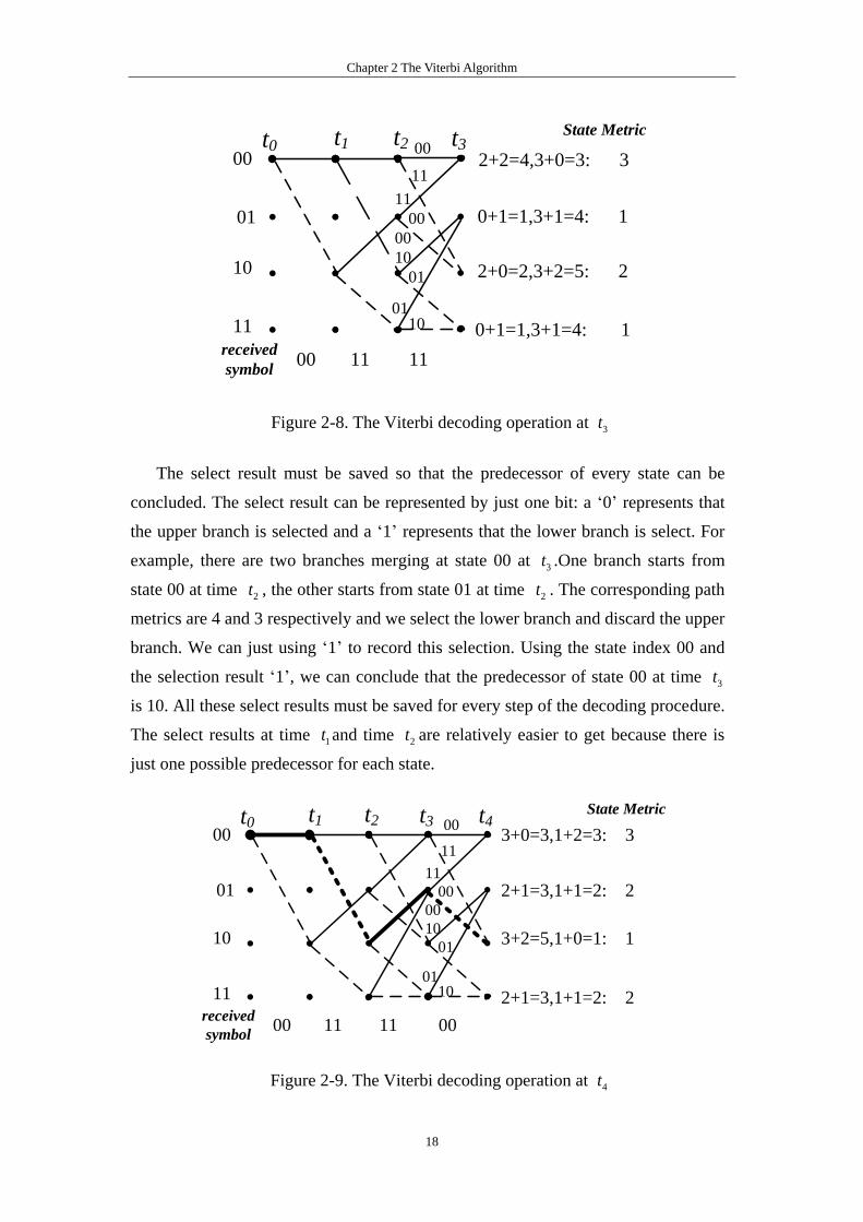
Figure 2-9. The Viterbi decoding operation at 4t

Chapter 2 The Viterbi Algorithm
19
The decoding operation at time 4t is the same as it at time 3t and is illustrated
in Figure 2-9. In this figure, the path with the smallest path metric is shown in bold.
We can see that the path is the same as the encoder‟s encoding path through time 0t
to time 4t , as Figure 2-5 shows. So, the error symbol received at time 3t can be
corrected if the section of path is included in the final survivor path.
Repeating the operation at time 3t until all the received symbols is treated. The
decoding process at time 17t is shown in Figure 2-10 below. In this figure, the path
with the smallest path metric is the same as the whole encoding path in Figure
2-5 .We can take this path as the final survivor path and trace back along it in the
trellis to find the information bits of the final survivor path. Those information bits
are the output of the Viterbi decoder, and the information bits before encoded by the
convolutional encoder have renewed. That is what we expect by using the Viterbi
decoding algorithm.
t0 t1 t2 t3 t4 t5 t6 t7 t8 t9 t10 t11 t12 t13 t14 t15
00 11 11 00 01 10 01 11 11 10 00 10 11 00 11received
symbol
00
01
10
11
10 11
t16 t17
State Metric
3
6
5
6
Figure 2-10. The Viterbi decoding operation at 17t
If the channel is Gaussian Channel, the Viterbi decoding procedure is very
similar as procedure introduced above. The biggest difference is the way to calculate
the branch metric. In this case, the Gaussian Distance can be the proper metric and
the ACSU should select the path with bigger path metric, as section 2.3.2 describes.
At the end of the section, it‟s better to discuss how to find the final survivor path
more efficiently. As stated above, the final survivor path is the path with maximum
likelihood among all the survivor paths. It implies that we should compare all the
states and select the one with the minimum state metric if the channel is BSC or
select the one with the maximum state metric if the channel is Gaussian channel. If
the constraint length of the convolutional codes is large, the state index will be very
large and the compare operation will be complex. So it‟s not practical to find the
final survivor path in this way.
The convolutional codes have a very useful characteristic which can help us to

Chapter 2 The Viterbi Algorithm
20
overcome this problem. If we start from every state and trace back along its survivor
path in the trellis, all the survivor paths will merge with high probability into a state
after D iterations. The number D is the well-known survivor path length and is
typically 5K [12]. Figure 2-11 below illustrates this characteristic.
Decisio
n
final survivor
path
survivor paths
trace back
the merging state
D>5KU
Figure 2-11. All the survivor paths merge after L iterations in the trellis

Chapter 3 The Soft Output Viterbi Algorithm
21
Chapter 3 The Soft Output Viterbi Algorithm
3.1 Original Formulation of SOVA
The Soft-Output Viterbi Algorithm (SOVA) is a modified Viterbi Algorithm
which can not only take in soft quantized samples but also provide soft decision
outputs along with the hard decision. The SOVA can generate the hard decision in
the same way as the Viterbi Algorithm. In addition, it can generate the reliability of
the hard decision, which is named as the Soft-Output. The Soft-Output can be
provided to its successor to improve the decoding performance of the concatenated
decoder.
At time kt , the ACSU in the Viterbi decoder selects a path with larger path
metric between the two paths merging at the same state s(It should be noticed that
SOVA requires soft input. So the ACSU in the decoder should select the path with
larger path metric). Without loss of generality, we assume path 1 is selected the
survivor (that is, the path metric of path is larger). The probability of selecting the
wrong path (path 2) as the survivor is
,
, ,,
- (2)
, , , ,- - (2) |) |(1
1 1 , | (2) (1) | 0
21s k
s k
s k s ks k s k s k s k
eP
e e e
≤ ≥ (3-1)
Where , (1)s k and , (2)s k is the path metric of path 1 and path 2 respectively [8].
The absolute value computation in Equation (3-1) can make the formula independent
of the actual path decision.
With probability ,s kP , the Viterbi decoder made errors in all the e positions where
the information bits of path 1 differs from path 2 (we can also say the decoder made
a relevant decision at these positions); in other words if
(1) (2)
1, ,...,j j eu u j j j (3-2)
As Figure 3-1 shows, there are two paths merging at state 00 at time 9t . Path 1 is
selected as the survivor path and its path metric is 23. Path 2 is discarded and its path
metric is 17.The discarded path can also be named as the competing path.
The information bits of path 1 is
(1) (1)
0 8~u u = 0 1 0 1 0 1 0 0 0.
The information bits of path 2 is

Chapter 3 The Soft Output Viterbi Algorithm
22
(2) (2)
0 8~u u =1 0 0 0 1 1 1 0 0.
So there are 5 positions where the information bit of path 1 differs from path 2, and
the Viterbi decoder made errors in those 5 positions with probability
-17
0,9 -23 -17 6
10.0025
1
eP
e e e
t0 t1 t2 t3 t4 t5 t6 t7 t8 t9
00
01
10
11
0
0
010
0
1
0
10
0
1
1
1
0
0
01
, (1) 23s k
, (2) 17s k , 6s k
j1 j2 j3 j4 j5
Path 1
Path 2
Surviving path
Competing path
Figure 3-1. An example of ,s kP
Assume the length before path 1 and path 2 merge is m . So there are e
different information values, and m e equal values. Assume the probabilities ^
jP
of previous erroneous decisions with path 1 have been stored. If path 1 is selected as
the survivor path, these probabilities for the e differing decisions on this path
according to the following equation
, , 1
^ ^ ^
) ), ,...( ,1 (1s k s kj ej jP P j jP P jP (3-2)
It is easily to demonstrate that ^
,0 0.5,s k jPP . Equation (3-2) requires that ^
jP and ,s kP are statistical independent. And it is approximately true for most of the
practical codes.
Both ,s kP and ^
jP are not suitable for hardware implementation. In practice, the
log-likelihood ratio ^
jL is used instead of ^
jP , which is defined as
^
^
^
1log
j
j
j
PL
P
(3-3)
Where ^
jL is named as the reliability of decision ju and it always has a
positive value. The bigger ^
jL is, the more reliable the decision ju is.

Chapter 3 The Soft Output Viterbi Algorithm
23
If the decision ju was relevant, its reliability ^
jL can be updated using the formal
value of ^
jL and the path metric difference of path 1 and path 2, ie, ,s k . The
updating formula is now
^
,
^ ^
,( , ) min( , )s k s kj j jL f L L (3-4)
Equation (3-4) is much easier to implement in hardware and does not deteriorate
the performance of the algorithm [8].
Figure 3-2 is an example showing how to update ^
jL . In this figure, path 1 and
path 2 merge at state 00 at time 5t , of which path 1 is selected as the survivor path.
The path metric difference of the two paths is 0,5 .
The information bits of path 1 is
(1) (1)
0 4~u u = 0 1 0 0 0.
The information bits of path 1 is
(2) (2)
0 4~u u = 1 1 1 0 0.
So we can see that information bits 0u and 2u are relevant and their reliability ^
0L and ^
2L need to be updated. Before being updated, all the reliability values ^ ^
0 4~L L have been initialized to a very large value at time 0t and some of them have
been updated at time 0 4~t t . At time 5t , only ^
0L and ^
2L needed to be updated and
the update equation is
0,5
^ ^
0,5
^ ^
0 0 2 2min( , ) min( , )L L and L L (3-5)
00
01
10
11
Path 1
Path 2
0
0
0
1
0
0
1
1
1 0,5
^
0L^
2L^
1L^
3L^
4L
update update
t0 t1 t2 t3 t4 t50
Survivor path
Competing path
Figure 3-2. An example of updating operation

Chapter 3 The Soft Output Viterbi Algorithm
24
3.2 Two-Step SOVA
The original SOVA, as introduced above, requires the construction of a
competing path for all states and performing the update operation along the paths for
all states. However, the final hard output of the decoder is only the information bits
of the final survivor path. Thus, all update operations that are performed on
reliability values that are not associated with the final survivor path do not affect the
output of the decoder.
C.Berrou [9] in 1993 proposed a new architecture named two-step SOVA which
can implement the SOVA more efficiently. It splits the SOVA into two steps and
discards the unnecessary update operations. In the first step, the common Viterbi
algorithm is employed to find the final survivor path and generate the final hard
decision. The update operation is postponed to the second step when the final
survivor path is known. This causes at least a delay of D steps if D denotes the
survivor depth of the SMU. Subsequently only the reliability values associated with
this path are updated with respect to the competing paths constructed for each
decoding step.
Figure 3-3 is an example of Two-Step SOVA. In the first step, we start tracing
back in the trellis from an arbitrary state in time kt , usually from the all-zero state.
After D iterations along the survivor path, the path will end in the merging state at
time k Dt , which is state 10 in this example. In the second step, the reliability values
of the relevant bits among the U information bits (in this example, U is 4 for
simplification) have been updated. (1)
2k Du and (2)
2k Du is relevant so 2k DL
has to
be updated using the following equation
^ ^
2 2 2,( , )k D k kD DL min L (3-6)
At time kt , the update operation of the reliability value k D UL
is completed and
can be output as the soft information associated with the hard decision k D Uu .Note
that the first 1K (in this example, 1K =2) branches in this example have
identical labels. This is always the case if a feed forward encoder is used and can be
exploited since the decision about the paths is never relevant with respect to these
symbols.

Chapter 3 The Soft Output Viterbi Algorithm
25
ktk D Ut
……
k Dt
2k DLupdate
first stepsecond step
2,k D
00
01
10
11
the final survivor path
the competing path the merging state the survivor paths
0 0 01
101
Figure 3-3. An example of Two-Step SOVA
It is clear that update operation in a SOVA decoder takes place in a modified
survivor memory unit. The rest of the Viterbi decoder remains unchanged as
compared to a hard deciding Viterbi decoder except the ACSU. The ACSU now
have to not only select the survivor path, but also output the path metric difference of
the survivor path and its competing path. Since the metric differences are normally
already present inside the ACSU, no additional hardware is required.

Chapter 4 Hardware Architecture of SOVA Decoder
26
Chapter 4 Hardware Architecture of SOVA Decoder
Figure 4-1 is the architecture of the two-step SOVA decoder. The 3 modules in
the dotted square construct a hard deciding Viterbi Decoder. Note that the SMU here
has to output the state sequence in the final survivor path so that the update
processing can be carried out. And it should be noted that the decision bits and path
metric difference generated by the ACSU must be delayed to adjust the timing to the
outputs of the SMU.
Hard deciding Viterbi Decoder
inputSMU
PCU
,s kdec
relevance bits
MU
X
BMU ACSU
Delay
line 1
……
RMU
……
hard output
soft output
,s k Dd
,s k D
,s k
k Du
k D Uu
k D UL
,s k DS
Delay
line 2
( )quantized symbols
Figure 4-1. Architecture of Two-Step SOVA decoder
ACSU is a key module in the decoder and always limits the throughput of the
decoder. In this thesis, we adopt the modified CSA structure to implement the ACSU
so that the critical path delay of ACSU can be decreased greatly. And by using
seven-level quantization instead of the conventional eight-level quantization to
quantize the input symbol, we can use only 8 bits instead of 9 bits to represent the
path metric, which can save the hardware overhead of the decoder and further
decrease the critical path delay of ACSU. See section 4.2 and 4.3 for the detailed
description.
The two delay lines, especially the delay line storing the path metric difference
of every state, contain the major portion of the overall required memory. The depth
of memory used in the delay line is determined by the decode latency of SMU. For
example, if the path metric difference is presented using 7 bits and the memory depth
is 60, the depth of memory used in the delay line should be 64 (It should be noted
that the depth of memory must be the integral power of 2.) and the total bits in the

Chapter 4 Hardware Architecture of SOVA Decoder
27
delay line 1 will be 64 64 7 28672 . And if the memory depth has to be
increased to 105, we need another 28672 bits to store these path metric differences!
So, the SMU must be designed carefully to save the memory used. In section 4.4,
two novel SMU architectures are proposed and one of them is applied to the SOVA
decoder. They both can make sure the decode latency be less than 64 without
consuming two much power.
In section 4.5, we proposed an optimized architecture of PCU by removing the
unnecessary stages and XOR gates. The optimized architecture can save about half
of the hardware overhead without decreasing the decoding performance. And the
architecture of RMU can also be optimized using the similar method. Section 4.5 and
4.6 will discuss this method in detail.
The detail of the hardware architecture will be described in the left part of the
chapter. Before the description, the convolutional codes used in the ECMA-368
UWB standard (we‟ll call it the UWB standard for short in the left part of the thesis)
should be introduced because it will affect the design of the SOVA decoder.
4.1 Convolutional Codes in the UWB Standard
Figure 4-2 shows the convolutional encoder employed in the UWB standard. The
constraint length and code rate of the codes it generates is 7K and 1/ 3R
respectively. And the generator polynomials of the encoder is 0 8133g , 1 8165g ,
and 2 8171g . The bit denoted as “A” shall be the first bit generated by the encoder,
followed by the bit denoted as “B”, and finally, by the bit denoted as “C”.
D D D DD D
output 0
output 2
input
output 1
+ +
+
+
+
+
+ +
+
+ +
+
Figure 4-2. Convolutional encoder in the UWB standard
Additional code rates are derived from the “mother” rate 1/ 3R convolutional
code by employing “puncturing”. Puncturing is a procedure for omitting some of the
encoded bits at the transmitter (thus reducing the number of transmitted bits and
increasing the code rate) and inserting a dummy “zero” metric into the decoder at the

Chapter 4 Hardware Architecture of SOVA Decoder
28
receiver in place of the omitted bits. The puncturing patterns are defined in Figure
4-3 to Figure 4-5 [1]. In each of these cases, the tables shall be filled in with encoder
output bits from left to right. For the last block of bits, the process shall be stopped at
the point at which encoder output bits are exhausted, and the puncturing pattern
applied to the partially filled block.
Source Data
Encoded Data
Bit Inserted Data
0x
0A0C
0A
0B
0C
0A
0B
0C
0y
Stolen Bit
Inserted
Dummy Bit
Bit Stolen Data
(sent/received data )
Decoded Data
Figure 4-3. An example of bit-stealing and bit-insertion for 1/ 2R code
0A0B 1C 2A
2B 3C 4A 4B
0A 1A 2A 3A 4A
0B 1B 2B3B 4B
0C 1C 2C 3C 4C
0A 1A 2A 3A 4A
0B 1B 2B3B 4B
0C 1C 2C 3C 4C
0x 1x2x 3x 4x
0y 1y2y 3y 4y
Source
Data
Encoded
Data
Bit Inserted Data
Bit Stolen Data
(sent/received data )
Decoded Data
Stolen Bit
Inserted
Dummy Bit
Figure 4-4. An example of bit-stealing and bit-insertion for 5 / 8R code

Chapter 4 Hardware Architecture of SOVA Decoder
29
0A0B 1C 2C
1x2x 3x
1y2y 3y
0A 1A 2A
0B 1B 2B
0C 1C 2C
0A 1A 2A
0B 1B 2B
0C 1C 2C
Source Data
Encoded Data
Bit Inserted Data
Bit Stolen Data
(sent/received data )
Decoded Data
Stolen Bit
Inserted
Dummy Bit
Figure 4-5. An example of bit-stealing and bit-insertion for 3/ 4R code
The UWB standard supports 8 kinds of data rates ranging from 53.3 Mbps to 480
Mbps, as Table 4-1 shows. For data rates not greater than 200 Mbps, the binary
information shall be modulated by the quadrature phase shift keying (QPSK)
modulator. For data rates greater than 320 Mbps, the binary data shall be modulated
using a dual-carrier modulation (DCM) technique. The rate-dependent code rate and
modulation parameters are listed in Table 4-1.
Table 4-1 The convolutional codes in ECMA-368
Data Rate (Mbps) Code Rate Modulation
53.3 1/3 QPSK
80 1/2 QPSK
106.7 1/3 QPSK
160 1/2 QPSK
200 5/8 QPSK
320 1/2 DCM
400 5/8 DCM
480 3/4 DCM

Chapter 4 Hardware Architecture of SOVA Decoder
30
4.2 Branch Metric Unit
The punctured Viterbi decoder is used for diverse code rates using one Viterbi
decoder. To implement the punctured Viterbi decoder, a de-punctured unit is added
in the front of the BMU. The de-punctured unit takes in the input symbols and the
code rate mode signal, and the input symbol is then changed to an appropriate
symbol by a de-punctured metric.
Denote iZ as the i th branch of the received sequence after quantization, that is,
the received symbols at time it .And denote ijz as the jth code symbol of iZ .
Assume kC is one of the particular codeword which consists of three binary bits
{ 2c , 1c , 0c }. The corresponding octal number of the three bits is k , that is
2 1 0
2 1 02 2 2k c c c (4-1)
So, one of the eight branch metrics at time it can be computed as
2
0
( ) , 2 1i ji j j j
j
k z u where u c
(4-2)
Since uj is +1 or -1, no multiplier is needed to implement the Equation (4-2).
As section 2.3.2 shows, ijz can be quantized to one number belonging to a set
of numbers { 7, 5, 3, 1,1,3,5,7} . So that the value of ( )i k will range from -21
to 21. As the following section shows, this requires at least 10 bits should be used to
represent the path metric. Since reducing the bits needed to represent the path metric
can reduce the hardware overhead and speed up the ACSU, we should find a method
that can narrow the range of the branch metric.
One efficient scheme is to use seven-level quantization instead of the traditional
eight-level quantization. The quantized symbols then will belong to
{ 3, 2, 1,0,1,2,3} and the value of ( )i k will range from -9 to 9. By doing this,
the bits needed to represent the path metric can be decreased to 9 bits. When using
the seven-level quantization, we can just use 4‟b0000 to represent the punctured
symbols. And the “product” term ji jz u will be zero if jiz corresponds to a
punctured bit. In this way, we can still use the Equation (4-2) to compute the branch
metric without any modification.
Figure 4-6 shows, using the seven-level quantization instead of eight-level
quantization will only bring in an little loss in the decoding performance (In these
three figures, the trace-back length is set to 35. And we only give the simulation

Chapter 4 Hardware Architecture of SOVA Decoder
31
results of the 3 kinds of code rate corresponding to QPSK modulation.). Compared
to the hardware overhead reduction and speed increase it can bring in, this
performance loss is worthy.
(a) 1/ 3R
(b) 1/ 2R

Chapter 4 Hardware Architecture of SOVA Decoder
32
(c) 5 / 8R
Figure 4-6. Seven-level quantization VS eight-level quantization
Equation (4-2) can be revised as
2
0
( ) 9, 2 1i ji j j j
j
BM k z u where u c
(4-3)
In this way, the value of branch metric will always be nonnegative number.
The BMU can be easily implemented using some adders and subtracters (which
is also adder in essence). The widths of the quantized symbols that are input to the
BMU are all 4 bits and the output branch metrics are 5bits wide. The detail of its
architecture is omitted here.
4.3 Add-Compare-Select Unit
4.3.1 ACS VS CSA
ACSU is a key module in the hard deciding Viterbi decoder and SOVA decoder.
The ACS operation is recursive and is always the speed bottleneck of the decoder.
The ACS operation at time it can be expressed by the following two equations
0 0 0 0 1 1 0
1 1 1 1max{ , }x x x x x
i i i i i (4-4)

Chapter 4 Hardware Architecture of SOVA Decoder
33
1 0 0 1 1 1 1
1 1 1 1max{ , }x x x x x
i i i i i (4-5)
In the two equations, x stands for an arbitrary 5-bits number and is the
branch metric. Figure 4-6 shows the ACS operation using the trellis diagram. In this
figure, the state 0x and 1x at time 1it will transfer to state x0 if the current input is 0.
The state metric of the two state at time 1it is 0
1
x
i and 1
1
x
i respectively and the
branch metric of the two transition is 0 0x
i and 1 0x
i . At time it , the ACSU will
accumulate the path metric and its corresponding branch metric, and then select the
larger one as the state metric of state x0. Meanwhile, the ACSU should output the
decision of the selection and the path metric difference of the two paths ( 0,x i in
Figure 4-7).
0
1
01
1
x
i
0x
i
1x
i
0 0x
i
1 0x
i
0 1x
i
0
1
x
i
it1it
0,x i
1,x i
1 1x
i
Figure 4-7. ACS operation in the trellis diagram
Figure 4-8 shows the hardware block diagram of the ACSU corresponding to the
ACS operation shown in Figure 4-7. The comparison is implemented through
subtraction, and the most significant bit (MSB) of the result selects the survivor path.
0x
i
0x
id
0 ,x i
Compare
0
1
x
i
1
1
x
i
0 0x
i
1 0x
i
Select
Figure 4-8. Block diagram of the ACSU

Chapter 4 Hardware Architecture of SOVA Decoder
34
Previous high-throughput implementations of the Viterbi decoder [4] unrolled
the ACS loop in order to perform two-step iterations of the trellis recursions within a
single clock cycle. These look-ahead methods replace the original radix-2 trellis (As
Figure 4-7 shows) with a radix-4 trellis (See in Figure 4-9), at the cost of increased
interconnect complexity.
0
1
2
3
4
5
6
7
0
1
2
3
4
5
6
7
0
1
2
3
4
5
6
7
0
1
4
5
2
3
6
7
0
2
4
6
1
3
5
7
0
1
2
3
4
5
6
7
0
1
2
3
4
5
6
7
0
2
4
6
1
3
5
7
2it 1it it 2it 1it it 2it it
Figure 4-9. The trellis diagram of radix-4 ACS
A radix-4 ACSU computes four sums in parallel followed by a four-way
comparison. In order to minimize the critical-path delay, the comparison is realized
using six parallel pair-wise subtractions of the four output sums. In general, the
critical-path delay is still larger than that of radix-2 ACSU .One main reason of this
is that the fan-out inside the radix-4 ACSU is larger than that inside the radix-2
ACSU. Another main reason is that the select logic in the radix-4 ACSU is more
complex. However, due to the doubled symbol rate, the effective throughput is
improved if this increase in delay is less than twofold. The block diagram of radix-4
ACSU is shown in Figure 4-10.
The critical path of the radix-2 ACSU consists of a two-input adder, a two-input
comparator and a multiplexer. E.Yeo [11] proposed a new architecture to implement
the add-compare-select function, of which the critical path consists only of a
two-input comparator and a multiplexer. Consider the Equation (4-4) and Equation
(4-5) again. They can be rewritten as Equation (4-6) and Equation (4-7) if we add
00x
i or 01x
i at both sides of them
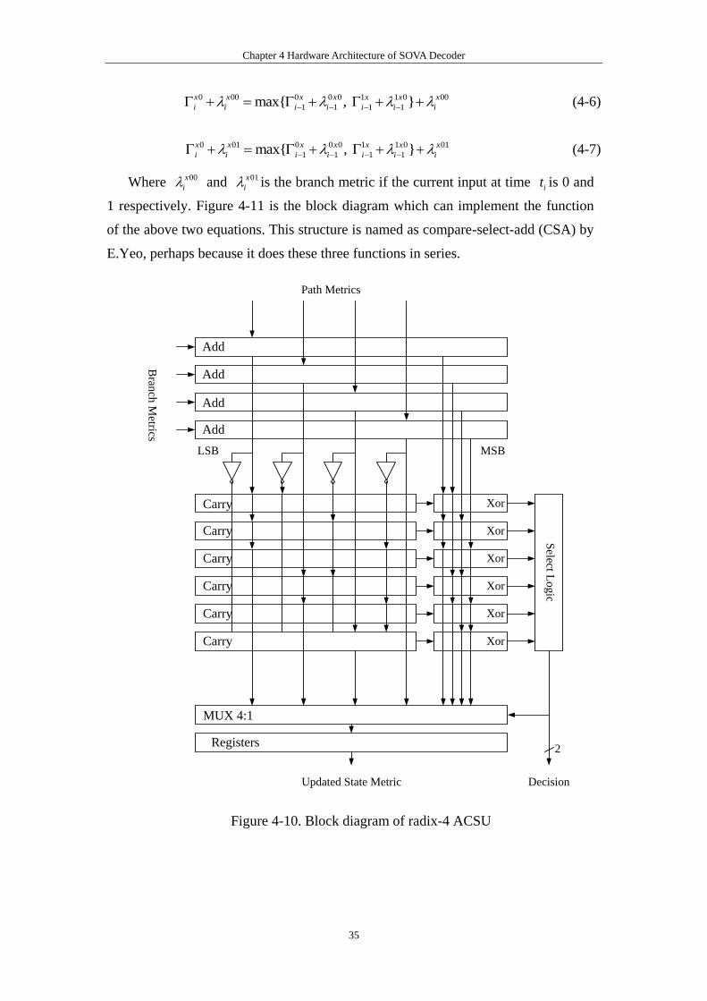
Chapter 4 Hardware Architecture of SOVA Decoder
35
0 00 0 0 0 1 1 0 00
1 1 1 1max{ , }x x x x x x x
i i i i i i i (4-6)
0 01 0 0 0 1 1 0 01
1 1 1 1max{ , }x x x x x x x
i i i i i i i (4-7)
Where 00x
i and 01x
i is the branch metric if the current input at time it is 0 and
1 respectively. Figure 4-11 is the block diagram which can implement the function
of the above two equations. This structure is named as compare-select-add (CSA) by
E.Yeo, perhaps because it does these three functions in series.
Select L
og
ic
Add
Add
Add
Add
Carry
Carry
Carry
Carry
Carry
Carry
Xor
Xor
Xor
Xor
Xor
Xor
MUX 4:1
Registers
MSBLSB
Path Metrics
Bran
ch M
etrics
Updated State Metric Decision
2
Figure 4-10. Block diagram of radix-4 ACSU

Chapter 4 Hardware Architecture of SOVA Decoder
36
0 0 0
1 1
x x
i i
1 1 0
1 1
x x
i i
01x
i
Compare
Select
0 00x x
i i
00x
i
0 01x x
i i
0x
id
0 ,x i
Figure 4-11. Block diagram of CSA structure
The CSA structure in the Figure 4-11 can be further modified by moving the add
operations before the select operation, resulting in the parallel execution of the
compare and add operations. The modified structure is shown in Figure 4-12. The
critical path delay is reduced to the combined delays of the comparator (The delay of
the comparator is slightly larger than that of the adder) and the multiplexer.
0 0 0
1 1
x x
i i
1 1 0
1 1
x x
i i
Select
0x
id
0 ,x i
01x
i
0 00x x
i i
0 01x x
i i
Select
Co
mp
are
00x
i
Figure 4-12. Modified structure of CSA

Chapter 4 Hardware Architecture of SOVA Decoder
37
E.Yeo showed by using the modified CSA structure to replace the conventional
ACS structure, the throughput can be increased by about 40%, at the cost that the
area and power will almost double. In contrast, by using the radix-4 ACS structure,
the throughput can be increased by about 60%, while area and power will increase
by about 5 times and 3 times respectively.
Thus, in this high-throughput SOVA decoder implementation, the modified CSA
structure is adopted because it provides much better balance between throughput and
power & area than the radix-4 ACS structure.
At the end of this section, we should discuss the way to generate the absolute
value of path metric difference. Since we don‟t need the reliability to be very
precise, we can generate the absolute value of path metric difference using an
approximate approach. For the two inputs of the comparator 0 0 0
1 1
x x
i i and
1 1 0
1 1
x x
i i , if 0 0 0
1 1
x x
i i is less than 1 1 0
1 1
x x
i i , the decision 0x
id is 1, and vice
versa. So the comparator can just subtracts the first input from the second input
and output the MSB (most significant bit) of the difference as the decision. If the
MSB of the difference is 0, we can use the other bits of the difference as the absolute
value of path metric difference. And if MSB of the difference is 1, we reverse each
bits of the difference and the result is the absolute value of path metric difference.
This can be easily implemented using some XOR gates, as the example in Figure
4.13 illustrates. In this example, the input diff is the difference of the substation with
[4]diff as its MSB. The delay of this structure is very less compare to the
multiplexer, so it will not affect the critical path delay of ACSU.
0, [3]x i
0, [2]x i
0, [1]x i
0, [0]x i
[4]diff
[3]diff
[2]diff
[1]diff
[0]diff
Figure 4-13. Example of the method to get the absolute value of path difference
4.3.2 Path Metric Normalization
As the Viterbi decoder operates continuously, the path metrics will grow

Chapter 4 Hardware Architecture of SOVA Decoder
38
proportional to the length on the received sequence. To avoid overflow or saturation
(depending on the number representation used), the path metrics need to be
normalized. There are basically two methods of doing this. Both rely on the
following two properties of the Viterbi algorithm [14]:
1. The maximum likelihood decoding path selection depends only on the metric
differences.
2. The metric differences are bounded.
Perhaps the most intuitionistic approach is to substrate the minimum path metric
from all the path metrics if the minimum path metric is large than a threshold.
Clearly, this does not affect the selection process because the path metric differences
remain the same. But doing this will make the decoding algorithm more difficult the
increase the critical path delay. Thus, it is not suitable in our design.
Another approach is the modular arithmetic method. It uses two‟s complement
arithmetic to calculate the path metric so that overflow can occur but it does not
affect the selection process. This approach is favored in hardware implementations.
Assume that two numbers a and b are compared using subtraction, and their
difference is less than , that is , | |a b . According to the number theory, the
comparison can be evaluated as mod( ,2 )a b without ambiguity. Hence, if the
path metric precision is chosen appropriately, the modular arithmetic can be
implicitly implemented by ignoring the path metric overflow.
Modular arithmetic also exploits the fact that the Viterbi algorithm inherently
bounds the maximum dynamic range max o f path metrics to be
max max 2log N (4-8)
Where N is the number of states (in this 64-state SOVA decoder, N is 64) and
max is maximum branch metric for the original radix-2 trellis.
So that the minimum path metric precision in the SOVA decoder is
2 max maxlog ( ) 1bits (4-9)
Where the operation A rounds the elements of A to the nearest integers
greater than or equal to A . The term max in the above equation accounts for the
potential dynamic range increase due to the use of the radix-2 CSA structure. In the
radix-2 CSA structure, the path metric and its corresponding branch metric are
treated as a whole.

Chapter 4 Hardware Architecture of SOVA Decoder
39
The equivalent of overflow errors will result if the design value for the dynamic
range is exceeded during operation. Hence, the upper bound given in Equation (4-8)
is used to ensure correct operation under all SNR conditions. If the eight-level
quantization is applied in this decoder, max will be 42 and bits will be 10. But if
we use the seven-level quantization as introduced in section 4.2, max can be reduced
to 18 and bits can be reduced to 8. Thus, we‟ll use seven-level quantization to save
the hardware cost and speed up the decoder.
Since the path metric can be presented using 8 bits, the path metric difference
can be presented using 7 bits.
4.4 Survivor Path Management Unit
There are two classical methods for survivor path management: the
register-exchange method and the trace-back method. Both methods require a
recursive update which fundamentally limits the throughput.
4.4.1 The Register-Exchange Method
The register-exchange method (RE) is the simplest and most direct method of
survivor path update and decode. A register exchange consists of a two-dimensional
array of one-bit registers and multiplexers. The registers in successive stages are
interconnected to resemble the trellis structure of the convolutional code [11][15].
Figure 4-14 is the structure of Register-Exchange SMU corresponding to the
convolutional encoder shown in Figure 2-1. The connection style of it is the same as
the trellis diagram shown in Figure 2-2.
Each row of registers records the decoded output sequence along the path from
the initial state to the final state. A global clock signal controls the registers. The
frequency of the clock determines the throughput of the Viterbi decoder. The
decisions from the ACSU ( 0d ~ 3d in the above figure) are input to select the outputs
of a corresponding row of multiplexers. At each clock cycle, a multiplexer located at
row i and column j outputs a decision bit corresponding to a trace-back of length
j , originating from state i . This bit is stored in a register and will be input to a
multiplexer at column 1j in the following clock cycle.

Chapter 4 Hardware Architecture of SOVA Decoder
40
00
01
10
11M
UX
MU
XM
UX
MU
X
MU
XM
UX
MU
XM
UX
0u
1u
2u
3u
0d
1d
2d
3dM
UX
MU
XM
UX
MU
X
1-bit register
State 3 survivor
path sequence
0
0
0
0
1
1
1
1
Figure 4-14. The structure of Register-Exchange SMU
The number of columns of array is survivor depth D . Given that the chosen
survivor depth is sufficiently large, there is a high probability that all survivors
merge and the symbol at depth D of any of the survivors may be chosen as output
symbols. We need to compute all survivors because they can affect the decoded
symbol sequence if a merge of paths occurs at depth D although the paths usually
merge earlier. So, the decode latency is identical to the survivor depth D . This is
the minimum decode latency we can achieve among all the different kinds of SMU
architectures we can use.
If the constraint length of the convolutional code is K, the survivor depth D
needs to be at least 5K . Since there are 12K columns in the array, the total
number of the registers and multiplexer will be as large as 15 2KK . At each clock
cycle, each survivor symbol sequence is completely overwritten with new survivor
symbols, resulting in 15 2KK read and write accesses per cycle. In our SOVA
decoder, the value of K is 7, so there will be as many as 2240 read and write
accesses per cycle. Thus, the power consumption is not acceptable if we take the RE
method.
4.4.2 The Trace-Back Method
The trace-back (TB) method is a backward processing algorithm for survivor
path update and decode. Such an algorithm is noncausal and requires the decisions to

Chapter 4 Hardware Architecture of SOVA Decoder
41
be stored in a decision memory prior to tracing back the survivor path. The current
state decision S
id is read from the decision memory using the current state iS and
time index i as an address. The previous state 1iS can be updated using iS and
S
id . For the common radix-2 trellis, we just need to right-shift iS by one bit with
S
id as the input of the shift register. Then the content of the shift-register is previous
state 1iS .
Practical trace-back architectures must achieve a throughput which is matched to
the throughput of ACSU while minimizing the required decision memory. The
one-pointer trace-back architecture described below is a practical implementation of
the architecture.
In the one-pointer trace-back architecture, the decision memory is organized as a
cyclic buffer and is partitioned into a write region and a read region as shown in
Figure 4-15. During each block decode phase, new decisions (one decision per state)
are written to the write region while the survivor path is traced and decoded from the
read region. The read region is divided into a merge block of length D and a
decode block of length U . Tracing-back through the merge block is used to find the
merging state from which the final survivor path starts. We can trace back along the
final survivor path in the decode block and get the hard deciding output. Once a
block is decoded it becomes the write block for the next phase and the other logical
partitions appropriately shift.
Decisio
n
final survivor
path
survivor paths
trace back
the merging state
DU U
Decode Block Merge Block Write Block
write
read region write region
Figure 4-15. Decision memory for trace-back architecture
To ensure continuous operation the trace-back operations must complete in the
time it takes to fill the write region. This requires more than one trace-back processes

Chapter 4 Hardware Architecture of SOVA Decoder
42
can be done every clock cycle. Thus, the frequency of the read pointer should be
several times (usually two or three) of that of the write pointer. This is not practical
in our SOVA decoder because the frequency of the read pointer is expected to be as
high as 480 Mega-Hz.
Another drawback of the one-pointer trace-back architecture is the large decode
latency. Assume we permit that multiple trace-back processes can be done every
clock cycle, the relationship between the length U and D is
11
DU where TRR
TRR
(4-10)
The decode latency is equal to the latency to fulfill the decision memory:
1
1
TRRlatency U D U D
TRR
(4-11)
The TRR in the above equations is the so-called trace-back recursion rate [15]. It
means the number of trace-back recursion per clock cycle.
In our SOVA decoder, the survivor depth D needs to be greater than 35. Thus,
if TRR is equal to 2, the minimum decode latency will be 105 clock cycles in the
write clock domain. And if TRR is equal to 3, the minimum decode latency will be
70 clock cycles in the write clock domain. As mentioned in the beginning of Chapter
4, the two delay lines in Figure 4-1 contain the major portion of the overall required
memory. Since the survivor depth should be greater than 35, the minimum decode
latency we can achieve is 35 clock cycles (It is only possible when the
register-exchange method is adopted. But according to the discussion above, the
register-exchange method is not suitable in our SOVA decoder.). So what we can do
to minimize the depth delay line is to make sure the decode latency be less than 64
cycles in the write clock domain. So the one-pointer trace-back architecture is not
practical in our SOVA decoder even if we permit that multiple trace-back processes
can be done every clock cycle.
4.4.3 The Trace-Forward Method
The purpose of tracing back through the merge block is to find the merging state.
But it will bring in two problems. First, it requires trace-back recursion rates greater
than one if want to decode continuously, which is very hard to implement in our
high-throughput SOVA decoder. Second, the delay of tracing back through the
merge block takes up a large proportion in the decode latency. A good solution to

Chapter 4 Hardware Architecture of SOVA Decoder
43
these problems is to use the hybrid trace-forward (TF) method [15].
The TF method combines the merits of both register-exchange method and
trace-back method. It enables us to find the merging state without tracing back in the
merge block. Instead, it estimates the merging state when the decisions are written to
the merge block. When the merge block is fulfilled with the newly input decisions,
the merging state is also found. So the latency of tracing back in the merge block is
eliminated and trace-back recursion rates can be reduced to one.
It is useful to define the tail of a survivor path before describing the TF method.
Every trellis state S at time it has an associated survivor path. Tracing back
through this survivor path and a certain state at time it can be found. That is called
the tail state of S and is denoted as ,
S
i iT . Thus, for L all the states at time
it have very large possibility to have the same tail state at time it . And this tail
state is the merging state we expect to find.
The TF method is a forward recursive procedure for finding the tail states over
the interval it to it . To do this, a register should be assigned to every state to
store its tail state and we name it as the tail state register in this thesis. When the
trace-forward operation starts at time it , the value of the tail state register is
initialized to its corresponding state index. This can be expressed as
,
S
i iT S (4-12)
The trace-forward update is merely a selection operation. The current state S at
time it will select its predecessor state 'S at time 1it according to its decision
value. And then, the content in the tail register of 'S is assigned to the tail register
of state S . Thus the updating function can be expressed using the following
equation
'
, , 1
S S
i i i iT T (4-13)

Chapter 4 Hardware Architecture of SOVA Decoder
44
ti ti+1 ti+2 ti+3 ti+4
00
01
10
11
titi+1 ti+2 ti+3 ti+4
00
01
10
11
( )a
00
01
10
11
01
00
10
10
10
10
00
00
00
00
10
00 00
00
00
00
( )b
tail state register
Figure 4-16. An example of trace-forward method
This update occurs concurrently for all states at time it and is similar in form to
the register-exchange method. Figure 4-16 shows an example of trace-forward
method. The survivor path for every state from time 1it to time 4it is shown in
Figure 4-14(a), where the survivor path of maximum likelihood at each time is
shown in bold lines. Figure 4-14 (b) shows how the tail state registers update their
values at each time. At time it , the tail state registers are initialized with their state
index. And from time 1it to time 4it , the register value for every state is updated
to the register value of the state‟s predecessor. As Figure 4-14(a) shows, every
state at time 4it has the same tail state 002 at time it , ie, all the survivor paths at
time 4it merge at state 002 at time it . Figure 4-14(b) shows that all the tail state
registers at time 4it have the same values 002. So, we can get the merging state at
time it immediately by reading from any one of these four register, without doing
the trace back operation.

Chapter 4 Hardware Architecture of SOVA Decoder
45
The decision memory can be organized similar to the one-pointer trace back
architecture except that all the three blocks must have the same depth, as shown in
Figure 4-17.
Decisio
n
final survivor
pathsurvivor paths
trace back
the merging state
LL L
Decode Block Merge Block Write Block
write
read region write region
trace-forward
Figure 4-17. Decision memory organization in the trace-forward architecture
During each block decode phase, new decision vectors are written to the write
region while the survivor path is traced and decoded from the read region.
Concurrently, the new decisions are processed by the trace-forward unit, which
estimates the state at the beginning of the each write block. Since the write block
becomes the merge block of the next phase, this state is the required starting state for
the next decode block.
At first glance the required decision memory length is 3L . However, because
the read and write rates are matched, the write block can be folded onto the decode
block, thus reducing the memory length to 2L . After a decision vector is read and
decoded, its location is available for the next written vector. Note that the decision
memory here is no longer a cyclic buffer and the read pointer and write pointer will
be a little more complex to control.
The architecture of trace-forward unit in a state-4 decoder (the corresponding
encoder is shown in Figure 2-1) is shown in Figure 4-18. It has the same connection
style with the trellis diagram. At time it each tail state registers is initialized with
its corresponding state index. On subsequent iterations, the interconnection and
multiplexers implement the recursive update under the control of the current
decisions. The trace-forward unit is busy updating the content of the tail state

Chapter 4 Hardware Architecture of SOVA Decoder
46
registers from it to it . At time it , the merging state can be found by reading
from any one of the registers. One of the update datapath is shown in red line in the
figure.
00
01
10
11
0d
2-bits register00
2d
3d
MU
XM
UX
MU
XM
UX
01
10
11
1d
update datapath
Initialize the register at the
beginning of TF operation
Figure 4-18. Architecture of trace-forward unit
4.4.4 The Modified Trace-Forward Architecture
If we apply the trace-forward architecture introduced above to our SOVA
decoder, the decode latency is still a problem. Assume that the length L takes its
minimum value 35, the decode latency will be 105L L L clock cycles. This is
unacceptable in our SOVA decoder. So modification needs to be done to the original
architecture.
Analyze the composition of the decode latency, we can find that the decode
latency can be reduced by shortening the depth of decode block. This mainly
because that fulfilling the decode block and tracing back in it will both bring a
latency whose value is equal to the depth of the decode block. An effective way is to
divide the three blocks into several smaller sections and use more than one
trace-forward unit.

Chapter 4 Hardware Architecture of SOVA Decoder
47
write
Time12 12 12 12 12
0t
12t
24t
36t
48t
4
60t
64bank0 bank1 bank2 bank3 bank4
bank0 bank1 bank2 bank3 bank4
writeTFU0
TF
bank0 bank1 bank2 bank3 bank4
writeTFU0
TFTFU1
TF
bank0 bank1 bank2 bank3 bank4
writeTFU0
TFTFU1TF
TFU1TF
bank0 bank1 bank2 bank3 bank4
writeTFU1
TFTFU2TF
TFU0TF
read,decode
Figure 4-19. Working flow of architecture A
In this thesis, two different kinds of survivor path architecture are developed.
They are both modified based on the trace-forward architecture mentioned above.
The working flow of the first architecture (It‟s named as architecture A below for
simplification) is illustrated in Figure 4-19. In this architecture, the memory
fragment of length 12 is treated as a whole. They are denoted as bank0~bank4 in the
figure. These banks are located in the same memory whose depth and width are both
64. It should be noted that the location of these 5 banks are not fixed in the memory.
The figure just shows their location from time 0t to 59t .

Chapter 4 Hardware Architecture of SOVA Decoder
48
In this architecture, a trace-forward unit will continue operate until a whole
merge block is fulfilled with newly input decisions. The merge block consists of
three banks whose length is 12. The operation details of this architecture are
described below.
The combination of bank1, bank2 and bank3 can be treated as the merge block if
we set bank0 as the decode bank. From time 0t to 11t , decisions are written to the
bank0. Since all the survivor paths originate from state 0 at time 0t , no
trace-forward operation is needed. From time 12t to 23t , decisions are written to the
bank1 and the first trace-forward unit denoted as TFU0 works. And from time 24t to
47t , TFU0 continues tracing-forward until bank3 is fulfilled with newly decisions (It
should be addressed that TFU0 needs not to be initialized at time 24t and time 36t .
It just continues tracing-forward based on the formal result.). After the 47th
clock
cycle passes, all the tail registers have stored the tail state at time 12t . And these
register are probable with the same value, which is just the merging state at time
12t .So, from time 48t to 60t , tracing-back can be done in bank0 with this merging
state as the start of final survivor path. From time 48t on, TF0 can be reused to trace
forward along with the other banks. The operation flow of the TF1 and TF2 is
similar to that of TF0.
The decode latency of this architecture is 60 clock cycles, which is less than 64
clock cycles and meets the requirements mentioned at the beginning of this chapter.
A drawback of this architecture is that three trace-forward units work concurrently
from time 36t on. Since a trace-forward unit consists of 264 1-bit registers and 64
2:1 multiplexers, the power consumption of this architecture is a big problem.
The other modified architecture, named as architecture B below, doesn‟t have this
problem. The working flow of architecture B is illustrated in Figure 4-20.
From time 0t to 11t , decisions are written to the bank0. And similar to the
working flow of architecture A, no trace-forward operation is needed during this
period. From time 12t to 23t , decisions are written to the bank1 and the first
trace-forward unit denoted as TFU0 works. After the 23th
clock cycle passes, the
TFU0 stops its operation for a while and the tail states at time 12t are stored in the
registers of TFU0. The tail registers in TFU1 are updated from time 24t to 35t . And
after the 35th
clock cycle passes, the TFU1 stops its operation for a while with the
tail states at time 24t stored in its tail state registers. From time 36t to 48t , the tail
states at time 36t are stored in the state registers of TFU2. The merging state at time

Chapter 4 Hardware Architecture of SOVA Decoder
49
12t can be found by “tracing-back” through the three sets of tail state registers. The
detailed operation is described below.
write
Time12 12 12 12 12
0t
12t
24t
36t
48t
4
60t
64bank0 bank1 bank2 bank3 bank4
bank0 bank1 bank2 bank3 bank4
writeTFU0
TF
bank0 bank1 bank2 bank3 bank4
writeTFU0
TFTFU1
TF
bank0 bank1 bank2 bank3 bank4
writeTFU0
TFTFU1TF
TFU1TF
bank0 bank1 bank2 bank3 bank4
writeTFU1
TFTFU2TF
TFU0TF
read,decode
Figure 4-20. Working flow of architecture B
After the 33th
clock cycle passes, a state‟s tail state at time 24t has been stored in
its tail state register in TFU2. At time 34t , we select an arbitrary one of the tail state
registers (for example, select the register of state 0) and use its value as the address
to read from the 64 tail registers of TFU1. We denote the output of this read
operation as _ _S merge temp .Thus _ _S merge temp is the tail state at time
24t corresponding to the survivor path at time 33t . Then, at time 35t , we use

Chapter 4 Hardware Architecture of SOVA Decoder
50
_ _S merge temp as the address to read from the 64 tail registers of TFU0. The
output of this read operation is the merging state at time 12t , which is denoted as
_S merge . Then, at time 36t , _S merge can be used as the starting state of tracing
back through bank0. From time 48t to 59t , TFU0 is reused to do the trace-forward
operation when the decisions are input to bank4.
The most left address of the memory is read at time 59t , so the decode latency is
also 60 clock cycles. After the 59th
clock cycles passes, bank0 will change its
location in the memory to cover the 12 addresses that are to be written in the next 12
clock cycles (that is, the most right 4 addresses and the most left 12 addresses).
It can be seen from the above description that not more than one trace-forward
unit works at the same time in architecture B. So it consumes much less power than
architecture A. The hardware overhead of architecture B is slightly bigger than that
of architecture A. In architecture B, “tracing back” in the three sets of tail state
registers is needed in order to find the merging state. When we decide to find the
merging state, we should know predecessor and successor of the current
trace-forward unit. So it‟s a more difficult to control the work flow of architecture A.
And to implement this special kind of tracing-back operation, a 6-bits 64-1
multiplexer should be placed following the three trace-forward units, which will
increase the hardware overhead of architecture B slightly compared to the
architecture A.
Another disadvantage of architecture B is that the survivor depth in architecture
B is 2 steps less than that in architecture A. the survivor depth in architecture B is
limited to 2 steps less than the depth of merge block, because “tracing back” in the
three sets of tail state registers consumes 2 clock cycles. In contrast, the survivor
depth in architecture A can be as same as the depth of merge block. Simulations
using MATLAB shows decoding performance is almost the same either architecture
is adopted.
In summary, we will apply architecture B to the SOVA decoder because it
consumes much less power at the cost of increasing slightly hardware overhead.
4.5 The Path Comparison Unit
In the Path Comparison Unit (PCU), the information bits of the competing paths
need to be compared in one clock cycle to generate the relevance bits for the

Chapter 4 Hardware Architecture of SOVA Decoder
51
Reliability Measure Unit (RMU) [11]. While the information bits of the final
survivor are already known (they are input to the PCU) the information bits of the
competing path must be calculated.
The register-exchange method used in the SMU provides a convenient way to
determine whether competing paths lead to equivalent decision bits or not. The two
inputs to each 2:1 multiplexer reflect the competing decisions, and a test for their
equivalence can be realized by the addition of an XOR gate at each multiplexer
location. M
UX
MU
XM
UX
MU
X
MU
XM
UX
MU
XM
UX
1-bit register
0
0
0
0
1
1
1
1
MUX MUXk DS
0,k Dd
1,k Dd
2,k Dd
3,k Dd
0,kRel1,kRel
Figure 4-21. Architecture of PCU
Figure 4-21 shows the first two stage of the PCU. The architecture of the other
stages is the same with the second stage and is omitted here. The decisions generated
by the ACSU are delayed by D clock cycles to match the timing of the final
survivor states generated by SMU. These delayed decisions are denoted as

Chapter 4 Hardware Architecture of SOVA Decoder
52
0,k Dd ~ 3,k Dd in the figure. The multiplexers at the top of the figure are used to select
the relevance bits according the final survivor states. In this figure, k DS represents
the final survivor state at time k Dt , where k means it is generated by SMU at time
kt .The first two relevance bits at time kt is denoted as 0,kRel and 1,kRel in the figure.
MU
XM
UX
MU
XM
UX
1-bit register
0
0
1
1
MUX2[0]k DS
0, 2k Dd
1, 2k Dd
2, 2k Dd
3, 2k Dd
2,kRel
MU
XM
UX
MU
XM
UX
3,kRel
MUX
Figure 4-22. Optimized architecture of PCU
Analyze the structure of Register-Exchange SMU, we can find the values of the
registers in the first 1K stages are fixed independently of the input decisions. For
example, in Figure 4-12, the values of the registers in the first stage are always 0 0 1
1 from the top downward. And the values of the registers in the second stage are
always 0 1 0 1 from the top downward. Furthermore, for the two paths merging at
the same state, the 1K information bits near the state are always the same (It is
easy to comprehend. Assume the state S can be denoted as 1 2 0...K Ks s s in binary.
In the trellis diagram, given the input sequence 0 2 1,..., ,K Ks s s , a path starting form
an arbitrary state will end at the state S . So, these 1K information bits of the

Chapter 4 Hardware Architecture of SOVA Decoder
53
two paths are both 0 2 1,..., ,K Ks s s .). Thus, the corresponding 1K relevance bits
are always zero. Figure 3-2 is an example of this characteristic, where path 1 and
path 2 merging at state 0 at time 5t have the same information bits 00 at time 4t
and 5t . So, the first 1K stages of PCU in Figure 4-21 can be removed with the
first 1K relevance bits fixed to 0.
On the other hand, for the two states which can be denoted as 2 00 ...Ks s and
2 01 ...Ks s in binary respectively, the two predecessors of them are the same. Thus, the
relevance bits corresponding to the two states are the same. So, we can remove half
of the XOR gates in the Figure 4-19 and reduce the bits width of multiplexers at the
top by one bit.
The optimized architecture of PCU is shown in Figure 4-20. Compared its
former, the optimized architecture saves considerable hardware overhead and
reduces considerable power consumption. It is demonstrated that 2K is sufficient
for the update depth U of PCU [11]. So the number of stages in Figure 4-22 can be
set to 1K , which is equal to 8 in our SOVA decoder.
4.6 The Reliability Measure Unit
The function of Reliability Measure Unit is to generate the soft output of the
SOVA decoder by selecting the minimum path metric difference according to the
relevance bits along the final survivor path. So it can be easily implemented by
connecting comparators and multiplexers in a pipeline. The architecture of the RMU
is shown in Figure 4-23. In this figure, every update stage consists of a register, a 2:1
multiplexer and a comparator which can choose the minimum input. The register
in the first stage is initialized to the maximum binary representation of the reliability
measure, which is 7‟b1111111 in our SOVA decoder.
MU
X
MIND
0,kRel
MU
X
MIND
MU
X
MIND
1,kRel1,U kRel
k D UL
,s k D
max
Figure 4-23. Architecture of RMU
As discussed in section 4.5, the first 1K relevance bits are always 0. Thus,

Chapter 4 Hardware Architecture of SOVA Decoder
54
the first 1K multiplexers will always choose the input from the preceding
register. So the above architecture can be optimized by removing the first 1K
stages. Figure 4-24 shows the optimized architecture.
MU
X
MIND
1,K kRel
MU
X
MIND
MU
X
MIND
,K kRel 1,U kRel
k D UL
, 1s k D K
max
Figure 4-24. Architecture of optimized RMU

Chapter 5 The Concatenated Decoder
55
Chapter 5 The Concatenated Decoder
Concatenated coding was introduced in 1966 by Forney [16]. It is a powerful
technique for creating error-correcting codes by combining two or more codes
sequentially. The primary reason for using concatenated codes is to achieve a low
error rate with an overall implementation complexity which is less than that which
would be required by a single decoding operation. Figure 5-1 is an example of
concatenated encoding and decoding. The stream from the information source is first
encoded in the outer encoder. The output of the outer encoder is then re-encoded by
the inner encoder before transmission. At the receiver the decoding order must be
reversed, and so the inner decoder is adopted first.
Information
Source
Outer
Encoder Modulator
Information
Destination
Outer
Decoder Demodulator
Channel
Inner
Encoder
Inner
Decoder
Figure 5-1. An example of concatenated encoding and decoding
The attractiveness of SOVA decoder enables us to find a way to deliver its soft
output to the Reed Solomon decoder. Surely this kind of concatenated decoder will
outperform conventional Viterbi-RS concatenated decoder. In this Chapter, we‟ll
study how to concatenate the SOVA decoder and Reed-Solomon decoder. An easy to
implement scheme which can work under various kinds of convolutional code rates
is proposed.
5.1 The Reed-Solomon Codes
In 1960, Irving Reed and Gus Solomon found a new class of error-correcting
codes that are now called Reed-Solomon (RS) codes [6]. Ever since its discovery,
Reed-Solomon codes have found many applications, including compact disc players,
deep-space applications and digital video broadcasting, etc.
Reed-Solomon codes are nonbinary cyclic codes with symbols made up of m-bit

Chapter 5 The Concatenated Decoder
56
sequences, where m is any positive integer greater than 2. If k is the number of
data symbols being encoded and n is the total number of code symbols in the
encoded block, the RS codes can be denoted as RS( , )n k . The number n and k
must obey the following constraint:
0 2 2m< k < n < (5-1)
For the most conventional RS( , )n k code, the relationship between n , k and
m is
( , ) (2 1,2 1 2 )m mn k t (5-2)
Where 2n k t is the number of parity symbols that are added at the end of k
symbols being encoded.
The RS(n,k) code is capable of correcting any combination of t or fewer errors.
One can say that the decoder has 2n k t redundant symbols to “spend,” which is
twice the amount of correctable errors. For each error, one redundant symbol is used
to locate the error, and another redundant symbol is used to find its correct value. So,
if the RS decoder knows the error‟s location in advance, it just needs one redundant
symbol to correct it. That is the erasure-correction capability of the RS codes. For
the RS( , )n k code, it can correct up to n k erasures within the block, no matter
where these erasures locate. RS codes can be designed to have any redundancy.
However, the increase of redundancy will lead to the increase of complexity to
implement the high-speed RS decoder. So, in practice, RS codes with redundancy no
greater than 8 are often adopted.
In practice, m is often selected as 8 so that the block length n will be 255
symbols. The codes with so large block length are not flexible to be processed in
other modules of the communication system. So, we often use shortened RS codes
by removing parts of the information symbols. For example, the UWB standard is
able to use RS codes of 23 encoded symbols, while still retaining the 8-bit symbol
structure of a length-255 code.
The shortened RS code the UWB standard uses can be described as RS(23,17). It
is obtained by shortening a systematic RS(255, 249) code. The method for
shortening is to force the first 232 information symbols to be zeros. Since these 232
symbols are known to the receiver, they are not transmitted. It should be noted that
the performance of the shortened RS code is no less than its un-shortened

Chapter 5 The Concatenated Decoder
57
counterpart.
The two codes can be both specified using the generator polynomial ( )g x over
the Galois field F [1]. ( )g x can be expressed as
66 5 4 3 2
1
( ) ( ) 126 4 158 58 49 117i
i
g x x x x x x x x
(5-3)
Where x F and the coefficients are given in decimal notation.
We are not going to elaborate how to generate the RS codes and how to decode
them in this section. See [6] [13] [17] for more information about the RS codes.
5.2 The Architecture of Concatenated Decoder
In the UWB standard, no interleaver is used between the inner code and outer
code, and thus, iterative decoding cannot be employed. The typical concatenated
decoder consists of a Viterbi decoder that delivers hard decisions at its output
followed by an errors-only or errors-erasure RS decoder. We hope the inner decoder
can output the soft information to the outer decoder, so the performance can be
improved. The SOVA decoder is a very suitable candidate for this kind of inner
decoder because of its low complexity. Since the SOVA decoder provides soft
information to the RS decoder, we hope that the RS decoder can accept these soft
outputs. There are several existing algorithms for soft decoding RS codes [18][19].
But unfortunately, the large alphabet size of the RS code precludes the use of
maximum likelihood decoders due to very high computational complexity. The
research of soft input RS decoder is out of the range of this thesis so we will only
research the method to concatenate SOVA decoder and hard input RS decoder.
As introduced in the above section, RS codes have the remarkable property that
they are able to correct any set of n k symbol erasures within the block.
Furthermore, the RS decoder is capable of correcting a block of symbols if the
number of errors ( )n error and the number of the erasures ( )n erasure among the
block satisfy the following expression
2 ( ) ( )n error n errsure n k (5-3)
According to the above expression, we can extend the error-correcting capability
of RS decoder by marking some of the unreliable symbols as erasures.
It should be noted that the soft output of SOVA decoder is the reliability per bit

Chapter 5 The Concatenated Decoder
58
while the reliability per byte is required by the RS decoder. So we have to develop a
strategy to convert the bit reliabilities to the symbol reliabilities. No optimum
transformation exists because the SOVA output is correlated [7].
A simple suboptimal approach is to use the minimum of the bit reliabilities
corresponding to a symbol as the symbol reliability. The idea is that, we regard a
symbol reliable only if all of its bits are reliable. We name it as the „min‟ approach
here.
Another suboptimal approach is to use the sum of bit reliabilities corresponding
to a symbol as the symbol reliability. This strategy assumes the SOVA outputs are
independent. So the symbol probability can be computed as the product of all the
corresponding bit probability. Since the bit reliability is the logarithmic ratio of the
bit probability, we can take the sum of the sum of bit reliabilities as the symbol
reliability approximately. We name it as the „sum‟ approach here.
Because no optimum transformation exists, we cannot mark the erasures in the
block absolutely correctly. So it‟s better to prepare several possible erasure vectors,
and select one vector from them to test whether the decoder can correct the errors.
For an erasure vector, a „1‟ means that the data symbol is to be replaced with an
erasure symbol, and a „0‟ means that the data symbol is passed unaltered. Before
constructing all the possible erasure vectors, we should first set up a list of the
locations of the least reliable symbols in a block of RS codewords to be decoded.
The values of the 23 bits in the erasure vector are assigned according to this list. If
the number of least reliable symbols in the list is denoted as ( )n unreliable , the total
number of possible erasure vectors ( )n vectors can be computed as ( )
( )
n erasure
n unreliableC .
Table 5-1 The combinations of errors and erasures
Number of errors Number of erasures Decoding Capability
3 0 3
2 2 4
1 4 5
0 6 6
According to Equation (5-3), the number of errors and erasures can be
configured as table 5-1. The decoding capability in the table is the sum of number of
errors and number of erasures. The RS decoder can achieve this number of decoding
capability only when all the erasures are marked correctly, which is not often the

Chapter 5 The Concatenated Decoder
59
case in practice.
Analyzing this table, the number of erasures should be 4 or 6 if we want to have
obvious improvement in the decoding performance. In this thesis, we set ( )n error
and ( )n erasure to be 1 and 4 respectively. This decision is made based on the
following two considerations.
First, by using this configuration, the decoding capability is only 1 less than the
maximum decoding capability. But one error can exist outside of the list of erasures.
This is very useful when we cannot locate the erasures absolutely correctly.
Second, the total number of possible erasure vectors ( )n vectors is attractive for
hardware implementation if the number of erasures is 4. If ( )n unreliable is 5, then
( )n vectors is 5. Only two copies of RS decoder are needed to ensure continuous
decoding. If the number of erasures is 6, ( )n unreliable should be at least 4 and more
copies of RS decoder are needed to ensure continuous decoding. The reason for this
is explained in detail below.
RS
Decoder(s)
Correctness
Checker
Re-decoding
Controler
SOVA
Decoder
Bit to Byte
Reliability
Converter
Bit to Byte
Decision
Converter
bL
u
BL
Erasure
Vector
Generator
eV
S
SOVA-RS Concatenated Decoder
Figure 5-2. Architecture of SOVA-RS concatenated decoder
The proposed architecture of the SOVA-RS concatenated decoder is shown in
Figure 5-2. The bit reliability bL
is packed into the byte reliability BL
in the
so-called Bit to Byte Reliability Converter. At first, the error-only RS decoding
mode is used. If the RS decoder succeeds in decoding the RS code words in this
mode, the decoding is finished and the corresponding information sequence is
delivered. The correctness of the decoded symbols is checked in the so-called
Correctness Checker, which is in essence the syndrome compute block of the RS
decoder. The syndrome is the result of a parity check performed on the input code
block to determine whether it is a valid member of the codeword set. If in fact it is a
member, the syndrome has value 0. Any nonzero value of syndrome indicates the

Chapter 5 The Concatenated Decoder
60
presence of errors.
If the RS decoder fails in the error-only RS decoding, it will turn into the
errors-and-erasures decoding mode. The RS decoder will accept an erasure vector
from the so-called Erasure Vector Generator every decoding round. If the RS
decoder fails in a decoding round, a new erasure vector will be provided to it until
the decoder succeed or all the possible erasure vectors have be tested.
Then let‟s calculate how many copies of RS decoders are needed to ensure
continuous decoding. Because the SOVA decoder is bit oriented and every block of
RS codes have 184 bits, the RS decoder should finish decoding in 184 clocks to
ensure continuous decoding.
The Correctness Checker needs 23 clocks to judge whether the current block of
RS decoding result is correct or not. And the decode latency of the RS decoder is 40
clock cycles [20], among which the syndrome computing takes 23 clocks. Because
input 23 symbols to the RS decoder keep the same in every decoding round, so we
need to do the syndrome computing for only 1 time. Thus an additional decoding
round will cost additional 40 clock cycles. And it should be noted that when the 184
hard decisions are output from SOVA decoder, the syndrome computing can be
carried out at the same time. So, if continuous decoding is expected, at most 4
decoding rounds can be done. So if ( )n unreliable is 5, we need two copies of RS
decoder working concurrently to ensure continuous decoding. And if ( )n unreliable
is increased to 6, at least 4 copies of RS decoder are needed to working concurrently.
The number of RS decoders will become unacceptable if ( )n unreliable is greater
than 6.
Figure 5-3 illustrates the decoding performance of the SOVA-RS concatenated
decoder if the code rate of the convolutional code is 1/3. The figure also shows the
decoding performance comparison when the two kinds of bit to symbol reliability
transformation approaches are used. In this figure, the block error rate (BLER),
instead of BER, is used to reflect the decoding performance of the concatenated
decoder. It can be seen that the „min‟ approach performs a little better than the „sum‟
approach. Using the „min‟ approach, the SOVA-RS concatenated decoder can
achieve about 0.35 dB additional coding gain than the Viterbi-RS concatenated
decoder when the BLER is 10-3
.

Chapter 5 The Concatenated Decoder
61
Figure 5-3. Decoding performance comparison of the two approaches
In both the two approaches, the Bit to Byte Reliability Converter can be
implemented with low complexity. But compared to the „sum‟ approach, the „min‟
approach has an advantage which can be used to save the hardware cost of the
SOVA decoder. In the „min‟ approach, we use the minimum of the bit reliabilities
corresponding to a symbol as the symbol reliability. So we can decrease the bits
needed to represent the path differences by replacing all the path difference values
greater than a certain threshold with the threshold. Thus the several most significant
bits to represent the path differences can be removed. Simulation results show only 4
bits are needed to represent the path differences without affecting the decoding
performance of the concatenated decoder. The corresponding threshold is 4‟b1111.
If the 3 most significant bits of a path difference value are not 3‟b000, then we set
the path difference to be 4‟b1111, otherwise, we only take its 4 least significant bits
to represent the path difference. In this way, 12288 bits can be saved in Delay line2.
So, in this thesis, we use the „min‟ approach to convert the bit reliabilities to the
symbol reliabilities.
Figure 5-4 shows the decoding performance will not have attractive

Chapter 5 The Concatenated Decoder
62
improvement if we increase ( )n unreliable to 6. The corresponding ( )n vectors will
be increased to 15 and the number of RS decoders will be unacceptable if we still
hope the concatenated decoder can decode continuously.
Figure 5-4. Decoding performance if ( )n unreliable is increased to 6
Figure 5-5 to Figure 5-6 show the decoding performance of the concatenated
decoder when the code-rate of the convolutional code is 1/2 or 5/8 (Because the
DCM modulation needs to divide the input data into groups of 200 bits. We don‟t
think it is compatible with the convolutional-RS concatenated codes. So we only test
the 3 kinds of code rate corresponding to QPSK modulation.). We can see from these
figures that the SOVA-RS concatenated decoder can achieve about 0.3dB~0.35dB
performance gain compared to the traditional Viterbi-RS concatenated decoder when
BLER is 10-3
. These figures also show that only about 0.05dB additional
performance gain can be achieved if ( )n unreliable is increased from 5 to 6. So, in this
thesis, the number of least reliable symbols is selected as 5.

Chapter 5 The Concatenated Decoder
63
Figure 5-5. Decoding performance, convolutional code rate 1/ 2R
Figure 5-6. Decoding performance, convolutional code rate 5 / 8R

Chapter 6 Implementation Results
64
Chapter 6 Implementation Results
The SOVA decoder designed in this thesis is modeled using the Verilog HDL,
which is a popular hardware description language. The Verilog HDL provides a
means of describing a digital system at a wide range of levels of abstraction, and, at
the same time, provides access to computer-aided design tools to aid in the design
process at these levels.
The Verilog model is organized as Figure 6-1 shows. In this figure, m_top_sova
is the top module of the SOVA decoder. It invokes 5 sub-modules: m_bmu, m_acsu,
m_smu_tf, m_pcu and m_rmu. These 5 sub_modules are the models of the BMU,
ACSU, SMU, PCU and RMU respectively. The sub-module m_abs is invoked by
m_acsu to calculate the absolute value the path metric approximately. And the
sub-module m_dpram is the model of dual port RAM.
m_rmum_acsu
m_top_sova
m_smu_tf m_pcum_bmu
m_abs m_dpram m_dpram m_dpram
Figure 6-1. Organization of the SOVA decoder model
The Verilog model is verified by using Questasim 6.4d, which is a popular tool
for simulation and verification. A MATLAB model of the SOVA decoder has been
built in advance. This MATLAB model is described similarly to the Verilog model,
so that most of the important signals in the Verilog model have their corresponding
variables in the MATLAB model. Thus the MATLAB model can help to debug the
Verilog model.
The verified Verilog model is synthesized on the Xilinx Virtex5 XC5VLX330
FPGA (field programmable gate arrays) by using ISE 10.1. The synthesize report
shows that the minimum clock period of the SOVA decoder is 2.91ns. The critical
path of the decoder is the tracing-back operation (including the “tracing-back”
operation among the tail state registers) in module m_smu_tf. This operation
requires selecting one bit from a 64-bit signal in one clock, which is very time
consuming when implemented on FPGA. Except for this operation, the CSA

Chapter 6 Implementation Results
65
operation in the module m_acsu has the second longest delay. Its delay is 2.55ns and
is about 13% less than the delay of the tracing-back operation. It‟s hard to
re-optimize the tracing-back operation to shorten its delay.
Table 6-1 shows the Place & Route report of the SOVA decoder when
implemented on Xilinx Virtex5 XC5VLX330 FPGA. The post Place & Route
simulation shows that the decoder can operate at the frequency as high as 200MHz.
Table 6-1 Place & Route report of the SOVA decoder
Device Utilization Summary
Slice Logic Utilization Used Available Utilization
Number of Slice Flip Flops 4,012 207,360 2%
Number of Slice LUTs 5,979 207,360 3%
Number of route-thrus 545 414,720
Slice Logic Distribution
Number of occupied Slices 2,085 51,840 4%
Number of LUT Flip Flop pairs used 6,539
IO Utilization
Number of bonded IOBs 18 1200 1%
Specific Feature Utilization
Number of BlockRAM/FIFO 36 288 12%
Total Memory used (KB) 1296 10,368 12%

Chapter 7 Conclusions
66
Chapter 7 Conclusions
This thesis describes the development and design of a high-throughput
low-power Soft-Output Viterbi decoder of constraint length 7K . The decoder
supports any code rate defined in the ECMA-368 UWB standard.
The input symbols to be decoded are quantized to seven levels instead of the
traditional eight levels. In this way, the number of bits needed to represent the path
metric can be reduced from 10 bits to 8 bits. Thus, the delay of ACSU, which is
often the throughput bottleneck of the decoder, can be decreased and its hardware
implementation overhead can also be reduced. The quantized symbols are calculated
in BMU to get the branch metrics, where only simple addition and subtraction is
needed to be carried out.
The throughput of the ACSU is increased in further by adopting the modified
CSA structure proposed by E.Yeo. Compared to the traditional ACS structure, the
delay of CSA structure is reduced by removing one adder from its critical path, at the
cost of doubling the hardware implementation overhead.
In the SOVA decoder, the delay line storing the path metric difference of every
state contains the major portion of the overall required memory. The depth of the
memory is determined by the decode latency of SMU. Two kinds of traditional SMU
architecture, the RE method and TB method, are introduced and compared. Both of
them are not suitable for our SOVA decoder. A novel hybrid survivor path
management architecture is proposed in this thesis. It is modified based on the
trace-forward method and combines the merits of RE method and TB method. This
hybrid survivor path management architecture can decode continuously so that high
decoding throughput can be obtained. And no more than one trace-forward unit work
concurrently, so the architecture will not consume much power.
The trellis diagram of the encoder is analyzed carefully and it‟s found that the
first 1K stages of PCU are unnecessary and can be removed without affecting the
decoding results. RMU is optimized in the same way.
The way to concatenate the SOVA decoder and RS decoder is also researched.
The RS codes used in the ECMA-368 standard is RS(23,17), which can correct
arbitrary 3 symbols errors among the code block. This thesis proposes an easy to
implement scheme to concatenate the SOVA decoder and RS decoder under various
kinds of convolutional code rates. The scheme uses a property of the RS decoder,

Chapter 7 Conclusions
67
that is, the decoding capability of RS decoder can be extended by marking some of
the symbols with least reliability as erasures, which is named as errors-erasures RS
decoding. Simulation results show that, using this scheme, the concatenated
SOVA-RS decoder can achieve about 0.35dB decoding performance gain compared
to the conventional Viterbi-RS decoder.
The decoder is implemented on Xilinx Virtex5 XC5VLX330 FPGA. The post Place &
Route simulation shows that the throughput of SOVA decoder can be as high as
200Mbps. However, in ECMA-368 UWB standard, the highest data rate is 480 Mbps.
This throughput requirement is supposed to be met through custom circuit design and
technology scaling.

Chapter 7 Conclusions
References
[1] Standard ECMA-368(3rd Edition). High Rate Ultra Wideband PHY and MAC
Standard. 2008
[2] J. Viterbi, “Error Bounds for Convolutional Codes and an Asymptotically
Optimum Decoding Algorithm,” IEEE Trans. Inf. Theory, vol. IT-13, pp.
260–269, Apr. 1967.
[3] P. J. Black and T. H.-Y. Meng, “A 140 Mb/s, 32-state, radix-4 Viterbi decoder,”
IEEE J. Solid-State Circuits, vol. 27, pp. 1877–1885, Dec. 1992.
[4] A. K. Yeung and J. Rabaey, “A 210-Mb/s, radix-4 bit-level pipelined Viterbi
decoder,” ISSCC Dig. Tech. Papers, pp. 88–89, Feb. 1995.
[5] P. J. Black and T. H.-Y. Meng, “A 1-Gb/s, Four-State, Sliding Block Viterbi
Decoder,” IEEE J. Solid-State Circuits, vol. 32, pp. 797–805, Jun. 1997.
[6] I. Reed and G. Solomon, “Polynomial codes over certain finite fields,” SIAM
Journal of Applied Mathematics, vol. 8, pp. 300–304, Jun.1960.
[7] J. Hagenauer, E. Offer, and L. Papke, “Matching Viterbi decoders and
Reed-Solomon decoders in a concatenated system,” in S. B. Wicker and V. K.
Bhargava, editors, Reed-Solomon Codes and Their Applications, pp. 242–271.
IEEE Press, New York, 1994. ISBN 0-7803-1025-X.
[8] J. Hagenauer and P. Hoecher, “A Viterbi algorithm with soft-decision outputs
and its applications,” In IEEE Global Telecommunications Conf., Nov. 1989, pp.
47.11-47.17.
[9] C. Berrou, P. Adde, E. Angui and S. Faudeil “A Low Complexity Soft-Output
Viterbi Decoder Architecture,” IEEE Int. Conf. Communications, vol. 2, pp.
737–740, May. 1993.
[10] O. J. Joeressen and H. Meyr, “A 40-Mb/s soft-output Viterbi decoder,” IEEE J.
Solid-State Circuits, vol. 30, pp. 812–818, Jul. 1995.
[11] E. Yeo, S. Augsburger, W. R. Davis, and B. Nikolic, “A 500-Mb/s Soft-Output
Viterbi Decoder,” IEEE J. Solid-State Circuits, vol. 38, pp. 1234–1241, Jul.
2003.
[12] J. Chen, M. P. C. Fossorier, S. Lin and C. Xu, “Bi-Directional SOVA
Decoding for Turbo-Codes,” IEEE communication letters, vol. 4, pp. 405–407,
Dec. 2000.
[13] Digital Communications: Fundamentals and Applications, 2nd
Edition, Bernard

Chapter 7 Conclusions
Sklar, University of California, Los Angeles. ISBN-10: 0130847887. ISBN-13:
9780130847881.
[14] A. P. Hekstra, “An alternative to metric rescaling in Viterbi decoders,” IEEE
Trans. Commum., vol. 37, pp. 1220–1222, Nov. 1989.
[15] P. J. Black and T. H.-Y. Meng, “Hybrid survivor path architectures for Viterbi
decoders,” in Proc. Int. Conf. Acoust. Speech, Signal Process, 1993, vol. 1, pp.
433–436.
[16] G. D. Forney, Jr. Concatenated Codes. MIT Press, Cambridge, MA, 1966.
[17] Stephen B. Wicker and Vijay K. Bhargava, “An introduction to Reed-Solomon
Codes,” in S. B. Wicker and V. K. Bhargava, editors, Reed-Solomon Codes and
Their Applications, pp. 1–16. IEEE Press, New York, 1994. ISBN
0-7803-1025-X.
[18] E. Berlekamp, “Bounded distance+1 soft-decision Reed-Solomon decoding”,
IEEE Trans. Inform. Theory, vol.42, pp.704-720, May 1996.
[19] R. Kotter, A. Vardy, “Algebraic soft-decision decoding of Reed-Solomon
codes,” in Proc. ISIT’2000, pp.61.
[20] Jian Zhang, Guangrong Fan, Jingming Kuang and Hua Wang, “A high speed
low complexity Reed-Solomon decoder for correcting errors and erasures,” in
Proc. ISCIT’2005,pp.1009-1012