A general-purpose parallel raster processing programming library test application using a geographic cellular automata model

This article was downloaded by: [Columbia University]On: 05 October 2014, At: 13:27Publisher: Taylor & FrancisInforma Ltd Registered in England and Wales Registered Number: 1072954 Registeredoffice: Mortimer House, 37-41 Mortimer Street, London W1T 3JH, UK

International Journal of GeographicalInformation SciencePublication details, including instructions for authors andsubscription information:http://www.tandfonline.com/loi/tgis20

A general-purpose parallel rasterprocessing programming library testapplication using a geographic cellularautomata modelQingfeng Guan a & Keith C. Clarke ba Center for Advanced Land Management InformationTechnologies , School of Natural Resources, University ofNebraska-Lincoln , Lincoln, NE, USAb Department of Geography , University of California, SantaBarbara , Santa Barbara, CA, USAPublished online: 02 Mar 2010.

To cite this article: Qingfeng Guan & Keith C. Clarke (2010) A general-purpose parallelraster processing programming library test application using a geographic cellular automatamodel, International Journal of Geographical Information Science, 24:5, 695-722, DOI:10.1080/13658810902984228

To link to this article: http://dx.doi.org/10.1080/13658810902984228

PLEASE SCROLL DOWN FOR ARTICLE

Taylor & Francis makes every effort to ensure the accuracy of all the information (the“Content”) contained in the publications on our platform. However, Taylor & Francis,our agents, and our licensors make no representations or warranties whatsoever as tothe accuracy, completeness, or suitability for any purpose of the Content. Any opinionsand views expressed in this publication are the opinions and views of the authors,and are not the views of or endorsed by Taylor & Francis. The accuracy of the Contentshould not be relied upon and should be independently verified with primary sourcesof information. Taylor and Francis shall not be liable for any losses, actions, claims,proceedings, demands, costs, expenses, damages, and other liabilities whatsoever orhowsoever caused arising directly or indirectly in connection with, in relation to or arisingout of the use of the Content.

This article may be used for research, teaching, and private study purposes. Anysubstantial or systematic reproduction, redistribution, reselling, loan, sub-licensing,systematic supply, or distribution in any form to anyone is expressly forbidden. Terms &

http://www.tandfonline.com/loi/tgis20

http://www.tandfonline.com/action/showCitFormats?doi=10.1080/13658810902984228

http://dx.doi.org/10.1080/13658810902984228

Conditions of access and use can be found at http://www.tandfonline.com/page/terms-and-conditions

Dow

nloa

ded

by [

Col

umbi

a U

nive

rsity

] at

13:

27 0

5 O

ctob

er 2

014

http://www.tandfonline.com/page/terms-and-conditions

http://www.tandfonline.com/page/terms-and-conditions

A general-purpose parallel raster processing programming library testapplication using a geographic cellular automata model

Qingfeng Guana* and Keith C. Clarkeb

aCenter for Advanced Land Management Information Technologies, School of Natural Resources,University of Nebraska-Lincoln, Lincoln, NE, USA; bDepartment of Geography, University of

California, Santa Barbara, Santa Barbara, CA, USA

(Received 13 October 2008; final version received 21 March 2009)

A general-purpose parallel raster processing programming library (pRPL) was developedand applied to speed up a commonly used cellular automaton model with known tract-ability limitations. The library is suitable for use by geographic information scientists withbasic programming skills, but who lack knowledge and experience of parallel computingand programming. pRPL is a general-purpose programming library that provides genericsupport for raster processing, including local-scope, neighborhood-scope, regional-scope,and global-scope algorithms as long as they are parallelizable. The library also supportsmultilayer algorithms. Besides the standard data domain decomposition methods, pRPLprovides a spatially adaptive quad-tree-based decomposition to produce more evenlydistributed workloads among processors. Data parallelism and task parallelism are sup-ported, with both static and dynamic load-balancing. By grouping processors, pRPL alsosupports data–task hybrid parallelism, i.e., data parallelism within a processor group andtask parallelism among processor groups. pSLEUTH, a parallel version of a well-knowncellular automata model for simulating urban land-use change (SLEUTH), was developedto demonstrate full utilization of the advanced features of pRPL. Experiments with real-world data sets were conducted and the performance of pSLEUTHmeasured.We concludenot only that pRPL greatly reduces the development complexity of implementing a parallelraster-processing algorithm, it also greatly reduces the computing time of computationallyintensive raster-processing algorithms, as demonstrated with pSLEUTH.

Keywords: parallel computing; raster; cellular automata; SLEUTH

1. Introduction

1.1. Parallel computing for geospatial processing

Armstrong (2000) explicated that computational science has expanded the traditional viewof scientific frameworks to include modeling and simulation with a separate and equal role totheory and experimentation. He pointed out that geographers have been exploiting thebenefits of advances in computational science, and using modeling and simulation to gainunderstanding in geography for decades. However, computational complexity and pooralgorithmic performance has hampered the use of models to support scientific investigationand decision-making in geographic information science (GIScience). Saalfeld (2000) simi-larly considered computational complexity and intractability as the limitations of manygeographic information system (GIS) and cartography algorithms. Two trends in geospatial

International Journal of Geographical Information ScienceVol. 24, No. 5, May 2010, 695–722

*Corresponding author. Email: [email protected]

ISSN 1365-8816 print/ISSN 1362-3087 online# 2010 Taylor & FrancisDOI: 10.1080/13658810902984228http://www.informaworld.com

Dow

nloa

ded

by [

Col

umbi

a U

nive

rsity

] at

13:

27 0

5 O

ctob

er 2

014

mailto:[email protected]

http://www.informaworld.com

processing have caused an increase in computational complexity: the rapid increase in thevolume of geospatial and geography-related information, and the increased sophisticationand complexity of geospatial algorithms and models (Armstrong 2000). In many cases,researchers have to choose less-satisfying alternatives because the ‘best’ solutions appear tobe computationally infeasible. Undoubtedly, geospatial practitioners’ demand for comput-ing power will increase at an increasing rate.

Parallel computing, in contrast to sequential computing, is the use of multiple processingunits (computers, processors, and processes) working together on a common task in aconcurrent manner in order to achieve higher performance, usually measured by computingtime. A variety of parallel computing systems have been developed and brought intoapplications, including massive parallel computers, computer clusters, computationalgrids, and the recently emerged multi-core CPU computers. The adoption of parallelcomputing has widely spread in many fields, including weather forecasting, nuclearengineering, mineral and geological exploration, astrophysical modeling (Cosnard andTrystram 1995).

For geospatial practitioners, parallel computing provides a means to overcome computa-tional performance limits to solve geospatial problems in a shorter period of time, even tosolve problems that are computationally infeasible using sequential computing technology.Besides the high computational throughput, Ding and Densham (1996) pointed out that theprincipal benefit that geographers can obtain from parallel computing is ‘an improvedunderstanding of how to represent space and spatial relations and how to exploit them inanalytical procedures’. Openshaw and Turton (2000) also explained that modeling andsimulation based on parallel computing are more natural and realistic than sequentialmodeling because most geographical phenomena are results of multiple concurrent pro-cesses and their complex relationships.

Research on parallel GIS began more than 20 years ago, and many studies on geospatialapplications of parallel computing have been conducted, for example, in transportation andland-use modeling (Harris 1985), spatial data handling and analysis (Sandu and Marble1988, Li 1992), least cost path (Smith et al. 1989), polygon overlay (Wang 1993), terrainanalysis (Peucker and Douglas 1975, Rokos and Armstrong 1992, Puppo et al. 1994, Kidneret al. 1997), geostatistics (Armstrong and Marciano 1993, 1995–1997, Cramer andArmstrong 1997, Kerry and Hawick 1997, 1998, Wang and Armstrong 2003), and earthobservation (Aloisio and Cafaro 2003, Ananthanarayan et al. 2003). The research has movedin two main directions: parallelizing existing computationally intensive GIS operations anddeveloping new geospatial analytical methods using additional computational power(Clematis et al. 2003).

However, after more than two decades of research, it is still hard to say whetherthe discipline of geography, especially GIScience, has entered the high-performancecomputing (HPC) era, or, to be precise, the parallel computing era. An undeniable factis that most current geographical analytical tools and simulation models are still basedon sequential processing and completely outside the parallel computing world.Clematis et al. (2003) suggested that two factors ‘have had roles to play in obstructingthe rise of parallel GIS’: the inaccessibility of HPC resources and the lack of parallelGIS algorithms, application libraries, and toolkits. The first obstacle will eventuallydiminish in light of the newly emerged parallel computing technology that allowsGIScientists to either build inexpensive parallel computing systems (e.g., clustercomputing and multi-core CPUs) or access open HPC facilities (e.g., grid computingand cloud computing). The solution to the second obstacle may have the followingtwo dimensions.

696 Q. Guan and K.C. Clarke

Dow

nloa

ded

by [

Col

umbi

a U

nive

rsity

] at

13:

27 0

5 O

ctob

er 2

014

1. Even though some parallel geospatial algorithms and models have been developed,most of them are simple parallelism of algorithms and models. Very few existing parallelgeospatial algorithms and models have included the delicate load-balancing process, i.e.decomposing the data/tasks and mapping the subsets of data/tasks efficiently onto multipleprocessors. Thus, a study to compare existing load-balancing methods and even developspecial ones for parallel geospatial algorithms is necessary.

2. Because computer geospatial processes vary in data requirements, operation scope,and more importantly, workflow, it may be very hard for a generic parallel geospatialprogramming library or middleware to fully utilize parallel computing hardware for all thedifferent kinds of geospatial computing. On the other hand, designing and implementing aparallel algorithm requires extensive knowledge and experience of parallel computing andprogramming, which appears to be less possible for GIScientists. General-purpose parallelgeospatial programming libraries are in great need for current and future geospatial researchand applications, even though special parallelism of a specific algorithm or model mayachieve higher performance. Thus, if a generic parallel geospatial library is to be developed,it should be ‘general’ enough to allow users to develop their specific parallel algorithms fordifferent geospatial processes. In other words, a general-purpose library should greatlyreduce the development complexity of parallel algorithms and models without losingmuch performance improvement. Hutchinson et al. (1996) referred to the approach of hidingparallel computing details from nonspecialist users as the ‘transparent parallelism’ ofgeospatial processing.

This study aims to tackle these two aspects of the second obstacle by developing ageneral-purpose parallel geospatial programming library that provides users with multipleload-balancing options, including a workload-adaptive balancing mechanism. The uniquefeatures of this library, as well as some computational complexity and dependency analysisand considerations during the designing process, are presented in this article. Also, a parallelgeographic cellular automata (CA) model developed using this library is presented todemonstrate the usability and computational performance of this library.

1.2. Parallel raster processing

The raster data model, one of the most widely used data models for geospatial data,represents phenomena in geographical space as a grid of cells with attribute values(Duckham et al. 2003). This simple data structure is able to represent a large range ofcomputable geospatial objects, e.g., points, lines, areas, and surfaces or fields as a series ofdiscrete regular cells (Worboys and Duckham 2004). From a programming perspective, araster can be managed with ease in computers, because it can be mapped directly onto acomputer memory structure called the array (Clarke 2003b), and most commonly usedprogramming languages provide utilities to handle arrays (Worboys and Duckham 2004).The raster has been used as a primary data model for analytical geospatial processing andmodeling, e.g., land-use and land-cover change modeling, and terrain analysis and model-ing. The raster model has formed the basis of entire GIS software suites in the past, and todayit is at least supported as a storage and computational data structure in virtually all GISsoftware. Commonly stated advantages of the raster data model include the fact that thegeographic location of each cell is implied by its position in the grid; spatial analyses basedon neighboring cells are easy to program and quick to perform; the easy link to the layerconcept; large quantities of GIS data are already in this format (e.g., elevation data, imagery);and grid systems are compatible with raster-based output devices (Clarke 1995).

International Journal of Geographical Information Science 697

Dow

nloa

ded

by [

Col

umbi

a U

nive

rsity

] at

13:

27 0

5 O

ctob

er 2

014

From a parallel computing perspective, the raster was born to be parallelized. A rasterdata set is a matrix of values at a finite resolution, each of which represents the attribute of acorresponding cell on the land surface. Any matrix can be easily partitioned into sub-matrices and assigned to multiple processors for parallel computing.

However, in real-world applications, the processes can be much more complicated. First,the characteristics of the grids used in geospatial applications raise concerns for parallelcomputing. We define within raster processing a domain as the grid of cells or cellspace.There is a classic division within parallel computing between the partitioning of data acrossprocessors (i.e., data parallelism) and the partitioning of operations across processors (i.e.,task parallelism), with the result that both require an overhead of communications amongthe processors. To classify spatial processing and modeling from the data parallelismperspective, Ding and Densham (1996) defined two key characteristics: regularity andhomogeneity. The regularity of a spatial domain determines how easily it can be decom-posed geometrically into equal areas, whereas the homogeneity of the domain’s membersaffects the balance among partition workloads. A lack of homogeneity or regularity canincrease the communication cost, and lead to workload imbalances. For raster processing,the cellspaces are mostly of regular shapes (commonly squares and rectangles), whichimplies they can be easily divided into sub-cellspaces of equal areas. However, the cells ina cellspace may have different properties. In some applications, different types or values ofcells will be processed more or less frequently and so require differing computationalintensities across space. For example, when a line-thinning algorithm is applied to a cell-space of lines, only those cells that are identified as lines need to be processed, whereas othercells will be ignored. Heterogeneity in computational intensity over the cellspace is veryfrequently encountered in geospatial processing and creates workload imbalance among thesub-cellspaces, and so among the processors onto which the sub-cellspaces are assigned bydata parallelism.

Second, the scope of raster processing and modeling, which determines the range of datadependencies among sub-cellspaces, needs to be examined in parallel computing. Tomlin’s(1990) classification of map algebra is useful in classifying raster processing and modeling,and divides raster operations into those of local scope, neighborhood scope, regional scope,and global scope.

When a local-scope algorithm is used, e.g., selecting cells by attributes, each cell isprocessed in isolation. In this case a sub-cellspace only needs to hold the block of cells thatwill be processed by the algorithm. When a neighborhood-scope algorithm is used, forexample, calculating slopes and aspects from elevations, the computation for a given cellrequires the values of its neighborhood, a set of predetermined surrounding cells (sometimesincluding the cell itself). In consequence, a sub-cellspace has to hold not only the block ofcells to be processed, but also a ‘halo’ of cells surrounding the block (Mineter 1998). Initerative algorithms such as CA, the ‘halos’ of a sub-cellspace must be updated after eachiteration. Note that local-scope algorithms are special cases of neighborhood-scopealgorithms, those where the neighborhood contains only the cell to be processed itself.When a regional-scope algorithm is used, such as calculating the mean elevations of thestates in the United States, all the cells within a certain region are required in the computationfor the region. Two approaches to decomposition can be used (Mineter 1998). The firstdivides the cellspace by regions, which means a sub-cellspace holds the cells of a certainregion, but this approach is likely to lead to load imbalances as the regions differ in size. Thesecond approach divides the cellspace into regularly shaped sub-cellspaces, but extracomputation and communication have to be added to account for the region fragmentation.When a global-scope algorithm is used, all the cells in the cellspace are needed to generate


Dow

nloa

ded

by [

Col

umbi

a U

nive

rsity

] at

13:

27 0

5 O

ctob

er 2

014

the result. This kind of algorithm is the hardest to parallelize because it exhibits a large rangeof horizontal data dependence (Ding and Densham 1996).

To parallelize a raster-processing algorithm, the characteristics of the data sets (i.e.,regularity and homogeneity), and the nature of the algorithm itself (i.e., scope), have to betaken into account. If a general tool is to be developed for parallelizing raster algorithms, itclearly has to be sufficiently general to handle all kinds of data characteristics andprocessing scopes. Some efforts have been made to provide transparent parallelism ofraster processing. One example is the parallel raster-based neighbourhood modelling(NEMO) system developed at Carleton University in Canada (Hutchinson et al. 1996),which allows GIS researchers to easily parallelize three types of neighborhood modelingprocesses: neighborhood analysis, CA, and propagation. However, NEMO was specifi-cally developed for neighborhood-scope raster operations; a more generic parallel pro-gramming environment that supports all four types of raster processing in Tomlin’sclassification is still lacking.

In this study, an open-source general-purpose parallel raster processing programminglibrary called pRPL was developed in the C++ programming language to handle parallelcomputing processes for massive-volume raster processing. pRPL provides a simple butpowerful interface for users to parallelize almost any raster-processing algorithm as longas it is parallelizable, with any arbitrary neighborhood configuration. pRPL enables theimplementation of parallel raster-processing algorithms without requiring a deep under-standing of parallel computing and programming; thus it reduces the development com-plexity significantly. To demonstrate the advantages and performance of the library,a parallel geographic CA model, called pSLEUTH, was developed based on theSLEUTH urban growth and land-use change model (Clarke et al. 2007). pSLEUTH andtherefore pRPL were used to simulate and forecast urban growth over time. The goals wereto demonstrate the value of pRPL and get real-world performance data to evaluate ourapproach.

2. pRPL: an open-source general-purpose parallel raster processing programminglibrary

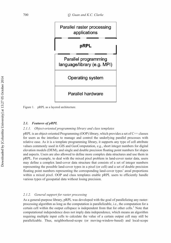
The goal in developing pRPL was to provide GIScientists who do not have experience withparallel computing with an easy-to-use development toolkit to parallelize their own raster-processing algorithms. From a software architecture perspective, pRPL serves as middle-ware connecting a general-purpose parallel programming library with application-specificraster-processing algorithms. pRPL hides the technical details of parallel computing fromthe users, thus relieving them from the time-consuming coding steps of parallel program-ming, and allowing them to focus on the algorithms themselves. Mineter and Dowers (1999)referred to this kind of architecture as a layered approach for the parallel processing ofgeographical applications (Figure 1).

pRPL was written in the programming language C++ and built upon message-passinginterface (MPI), a standard parallel programming library composed of a set of functions thatenable and manage parallel computing by passing messages among processors (Gropp et al.1998). MPI and C++ compilers are available on almost all parallel computing systems(e.g., massive parallel computers, computer clusters, and computational grids), so theportability of pRPL is guaranteed, and applications built upon it should be portable acrossdifferent parallel computing platforms. Furthermore, pRPL is an open-source programminglibrary and can be freely downloaded from http://sourceforge.net/projects/prpl/.


Dow

nloa

ded

by [

Col

umbi

a U

nive

rsity

] at

13:

27 0

5 O

ctob

er 2

014

http://sourceforge.net/projects/prpl

2.1. Features of pRPL

2.1.1. Object-oriented programming library and class templates

pRPL is an object-oriented Programming (OOP) library, which provides a set of C++ classesfor users as the interface to manage and control the underlying parallel processes withrelative ease. As it is a template programming library, it supports any type of cell attributevalues commonly used in GIS and GeoComputation, e.g., short integer numbers for digitalelevation models (DEM), and single and double precision floating point numbers for slopesand aspects. Users are also allowed to define more complex data structures and use them inpRPL. For example, to deal with the mixed pixel problem in land-cover raster data, usersmay define a complex land-cover data structure that consists of a set of integer numbersrepresenting the possible land-cover types in a pixel (or cell) and a set of double precisionfloating point numbers representing the corresponding land-cover types’ areal proportionswithin a mixed pixel. OOP and class templates enable pRPL users to efficiently handlevarious types of geospatial data without losing precision.

2.1.2. General support for raster processing

As a general-purpose library, pRPL was developed with the goal of parallelizing any raster-processing algorithm as long as the computation is parallelizable, i.e., the computation for acertain cell within the output cellspace is independent from that for other cells.1 Note thatcomputational independence does not imply data independence, which means an algorithmrequiring multiple input cells to calculate the value of a certain output cell may still beparallelizable. Thus, neighborhood-scope (or moving-window-based) and local-scope

Figure 1. pRPL as a layered architecture.


Dow

nloa

ded

by [

Col

umbi

a U

nive

rsity

] at

13:

27 0

5 O

ctob

er 2

014

algorithms are fully supported by pRPL, and some regional-scope and global-scope algo-rithms that meet the parallelizability criterion are also supported.

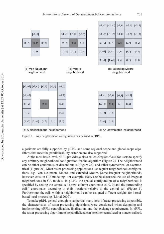
At the most basic level, pRPL provides a class called Neighborhood for users to specifyany arbitrary neighborhood configuration for the algorithm (Figure 2). The neighborhoodcan be either continuous or discontinuous (Figure 2d), and either symmetrical or asymme-trical (Figure 2e). Most raster-processing applications use regular neighborhood configura-tions, e.g., von Neumann, Moore, and extended Moore. Some irregular neighborhoods,however, exist in GIS modeling. For example, Batty (2000) discussed the use of irregularneighborhoods in CA models. In pRPL, the spatial configuration of a neighborhood isspecified by setting the central cell’s row–column coordinate as [0, 0] and the surroundingcells’ coordinates according to their locations relative to the central cell (Figure 2).Furthermore, the cells within a neighborhood can be assigned different weights for kernel-based local processing (Lloyd 2007).

To make pRPL general enough to support as many sorts of raster processing as possible,the characteristics of raster-processing algorithms were considered when designing andimplementing pRPL: centralization, finalization, and the exchange requirement. In pRPL,the raster-processing algorithm to be parallelized can be either centralized or noncentralized.

Figure 2. Any neighborhood configuration can be used in pRPL.


Dow

nloa

ded

by [

Col

umbi

a U

nive

rsity

] at

13:

27 0

5 O

ctob

er 2

014

A centralized algorithm evaluates and updates only the central cell of the neighborhood,whereas a noncentralized algorithm evaluates and updates any cell(s) within the neighbor-hood or the cellspace. Centralized algorithms are well supported by existing parallelneighborhood-scope raster-processing environments, e.g., NEMO. The support for noncen-tralized algorithms is, however, a distinctive feature of pRPL. This enables users to paralle-lize regional-scope and global-scope processing (e.g., linear feature tracing), as well as somespecial cases of neighborhood-scope processing. Examples of parallelizing noncentralizedalgorithms will be presented in the following case study. Also, in pRPL, a finalizing processcan be included in the algorithm, e.g., assigning a value to the cell based on an intermediatevalue of the cell calculated during the evaluation process. As mentioned before, an iterativeneighborhood-scope algorithm will require data-exchange processes among the sub-cellspaces after each iteration, which is handled by pRPL without any extra programmingon the user side.

When defining an application-specific raster-processing operation (termed Transition inpRPL), the user simply turns ON/OFF the options provided by pRPL to specify thecentralization (centralized/noncentralized), finalization (finalizing/nonfinalizing), andexchange (exchanging/non-exchanging) characteristics of the transition. The pRPL librarywill automatically optimize the underlying parallel computing routines according to thesecharacteristics.

pRPL also supports multilayer transitions. Multilayer processing is commonly used inraster-based geospatial algorithms, as well as in other kinds of image processing, forexample, an AND operation on two binary-coded images. pRPL allows users to use multipleLayer objects in a Transition, which implements the raster-processing algorithm, where eachLayer object may contain a cellspace and/or multiple sub-cellspaces. Once a cellspace in aLayer is decomposed, the sub-cellspace information (the locations in the global spatialextent and the local extents) can be used for other Layers so that they can be decomposedand distributed in exactly the same way so as to ensure the sub-cellspaces in multiple Layerswill match at geographical locations.

2.1.3. Regular and irregular decomposition

pRPL provides both regular and irregular decomposition methods to divide the domain(Figure 3). Regular decomposition divides the cellspace by rows, or columns, or blocks,without considering the workloads associated with the cells, producing equal-area sub-cellspaces. Regular domain decomposition methods have been widely used in parallelcomputing for numerical algorithms and image processing, where the workload is usuallyevenly distributed over the domain. Regular decomposition can also be used on hetero-geneous domains using the scattered decomposition technique (Mineter 1998). pRPL allowsusers to partition the domain into a large number of sub-cellspaces and lets each processorhold multiple sub-cellspaces scattered throughout the domain so as to increase the chance ofan even distribution of workload across the processors. However, scattered decompositionwill also increase the overhead of communication for data exchange in iterative algorithmsas the number of sub-cellspace increases. pRPL leaves the trade off between workloaddistribution and communication overhead to the user, allowing a choice of how many sub-cellspaces are produced in the decomposition process.

Irregular decomposition (or spatially adaptive decomposition), on the other hand, issuitable for the situation when the workload is clustered within the domain. Irregular decom-position takes into account the workloads of the cells, and is likely to produce unequal-areasub-cellspaces, but also likely to divide the workload more evenly among the sub-cellspaces.


Dow

nloa

ded

by [

Col

umbi

a U

nive

rsity

] at

13:

27 0

5 O

ctob

er 2

014

Irregular decomposition techniques for use in parallel raster processing already exist,e.g., hierarchies of irregular tessellations (Montanvert et al. 1991), and heuristic partitioning(Mineter 1998). pRPL provides a quad-tree-based (QTB) decomposition method, inspired byWang andArmstrong (2003).Wang andArmstrong used aQTB spatial domain decompositiontechnique for parallel point interpolation, where the number of control points within asubregion was used to determine the workload. The QTB decomposition is an iterativeprocess. The global cellspace (i.e., the root of the quad-tree) is initially divided into fourequal-area sub-cellspaces (termed leaves). Then, at each iteration, the workloads associatedwith the leaves are calculated, and the leaf with the largest workload is divided into four equal-area child leaves. The quad-tree keeps growing until the maximum number of leaves or theminimum workload associated with a sub-cellspace is reached. Note that the calculation ofworkload is a user-defined process (Section 2.2) and users have the freedom to designworkload-calculation algorithms according to their own raster-processing algorithms, whichis another distinctive feature of pRPL. Caution must be taken when the QTB decomposition isto be used, because the extra computation required to construct the quad-tree and to calculatethe workloads of the sub-cellspaces may outweigh the speed-up gained by a better workloaddistribution. Irregular decomposition is suitable for heterogeneous domains where the work-load is highly clustered. Therefore the QTB decomposition may not yield better performancethan other regular decomposition methods when the workload is rather scattered over thespace. Also, the workload of a sub-cellspace may change as the cell values change, thus theQTB decomposition is less preferable for iterative algorithms.

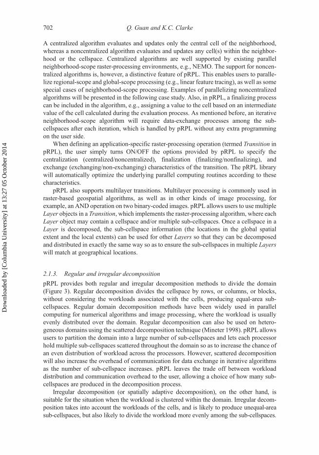
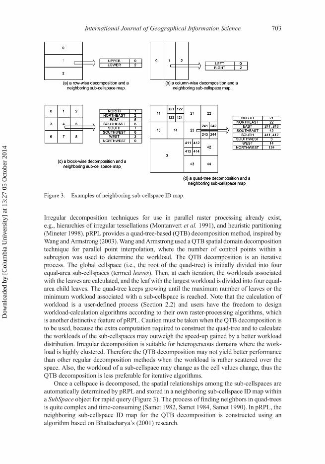
Once a cellspace is decomposed, the spatial relationships among the sub-cellspaces areautomatically determined by pRPL and stored in a neighboring sub-cellspace ID map withina SubSpace object for rapid query (Figure 3). The process of finding neighbors in quad-treesis quite complex and time-consuming (Samet 1982, Samet 1984, Samet 1990). In pRPL, theneighboring sub-cellspace ID map for the QTB decomposition is constructed using analgorithm based on Bhattacharya’s (2001) research.

Figure 3. Examples of neighboring sub-cellspace ID map.


Dow

nloa

ded

by [

Col

umbi

a U

nive

rsity

] at

13:

27 0

5 O

ctob

er 2

014

2.1.4. ‘Update-on-Change’ and the value-headed global-index stream for data exchange

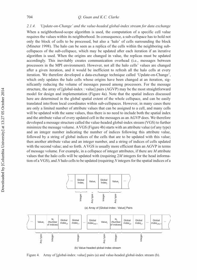
When a neighborhood-scope algorithm is used, the computation of a specific cell valuerequires the values within its neighborhood. In consequence, a sub-cellspace has to hold notonly the block of cells to be processed, but also a ‘halo’ of cells surrounding the block(Mineter 1998). The halo can be seen as a replica of the cells within the neighboring sub-cellspaces of the sub-cellspace, which may be updated after each iteration if an iterativealgorithm is used. When the origins are changed in value, the replicas must be updatedaccordingly. This inevitably creates communication overhead (i.e., messages betweenprocessors in the MPI environment). However, not all the halo cells’ values are changedafter a given iteration, and it would be inefficient to refresh all the halo cells at everyiteration. We therefore developed a data-exchange technique called ‘Update-on-Change’,which only updates the halo cells whose origins have been changed at an iteration, sig-nificantly reducing the volume of messages passed among processors. For the messagestructure, the array of [global-index : value] pairs (AGVP) may be the most straightforwardmodel for design and implementation (Figure 4a). Note that the spatial indices discussedhere are determined in the global spatial extent of the whole cellspace, and can be easilytranslated into/from local coordinates within sub-cellspaces. However, in many cases thereare only a limited number of attribute values that can be assigned to a cell, and many cellswill be updated with the same values, thus there is no need to include both the spatial indexand the attribute value of every updated cell in the messages as an AGVP does. We thereforedeveloped a message structure called the value-headed global-index stream (VGS) to furtherminimize the message volume. AVGS (Figure 4b) starts with an attribute value (of any type)and an integer number indicating the number of indices following this attribute value,followed by a string of global indices of the cells that are to be updated with this value;then another attribute value and an integer number, and a string of indices of cells updatedwith the second value; and so forth. AVGS is usually more efficient than an AGVP in termsof message volume. For example, in a cellspace of integer attributes, if there areM attributevalues that the halo cells will be updated with (requiring 2M integers for the head informa-tion of a VGS), andN halo cells to be updated (requiringN integers for the spatial indices of a

... ...GlobalIndexi

GlobalIndexj

Valuei

... ... ... ...Valuei ValuejGlobalIndexi,0

GlobalIndexi,1

GlobalIndexi,Ni-1

GlobalIndexj,Nj–1

GlobalIndexj,0

GlobalIndexj,1

Ni(Number

of indices)

Nj(Number

of indices)

(a) Array of [Global-index : Value] Pairs

(b) Value-headed global-index stream

Valuej

Inte

ger

Inte

ger

Any

type

Inte

ger

Any

type

Inte

ger

Inte

ger

Inte

ger

Any

type

Any

type

Figure 4. Array of [global-index: value] pairs (a) and value-headed global-index stream (b).


Dow

nloa

ded

by [

Col

umbi

a U

nive

rsity

] at

13:

27 0

5 O

ctob

er 2

014

VGS), then (2M + N) · sizeof(integer) bytes are needed for a VGS message, but2N · sizeof(integer) bytes are needed for an AGVP. When M is small and N is big (whichis usually the case), the VGS will be much smaller than the AGVP.

2.1.5. Non-blocking communication and ‘edgesFirst’ for data exchange

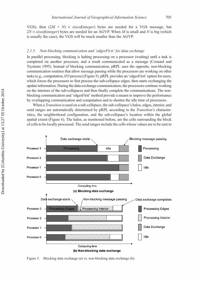
In parallel processing, blocking is halting processing on a processor (waiting) until a task iscompleted on another processor, and a result communicated as a message (Cosnard andTrystram 1995). Instead of blocking communication, pRPL uses the opposite, non-blockingcommunication routines that allow message passing while the processors are working on othertasks (e.g., computation, I/O process) (Figure 5). pRPL provides an ‘edgesFirst’ option for users,which forces the processors to first process the sub-cellspace edges, then starts exchanging theupdate information. During the data-exchange communication, the processors continueworkingon the interiors of the sub-cellspaces and then finally complete the communications. The non-blocking communication and ‘edgesFirst’ method provide a means to improve the performanceby overlapping communication and computation and to shorten the idle time of processors.

When a Transition is used on a sub-cellspace, the sub-cellspace’s halos, edges, interior, andsend ranges are automatically determined by pRPL according to the Transition’s character-istics, the neighborhood configuration, and the sub-cellspace’s location within the globalspatial extent (Figure 6). The halos, as mentioned before, are the cells surrounding the blockof cells to be locally processed. The send ranges include the cells whose values are to be sent to

Figure 5. Blocking data exchange (a) vs. non-blocking data exchange (b).


Dow

nloa

ded

by [

Col

umbi

a U

nive

rsity

] at

13:

27 0

5 O

ctob

er 2

014

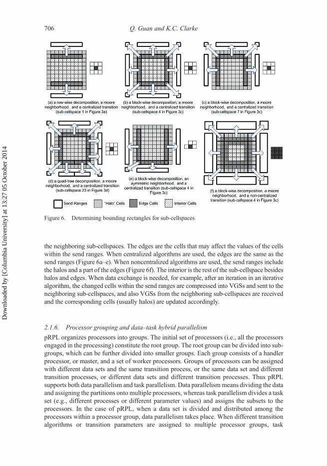
the neighboring sub-cellspaces. The edges are the cells that may affect the values of the cellswithin the send ranges. When centralized algorithms are used, the edges are the same as thesend ranges (Figure 6a–e). When noncentralized algorithms are used, the send ranges includethe halos and a part of the edges (Figure 6f). The interior is the rest of the sub-cellspace besideshalos and edges. When data exchange is needed, for example, after an iteration in an iterativealgorithm, the changed cells within the send ranges are compressed into VGSs and sent to theneighboring sub-cellspaces, and also VGSs from the neighboring sub-cellspaces are receivedand the corresponding cells (usually halos) are updated accordingly.

2.1.6. Processor grouping and data–task hybrid parallelism

pRPL organizes processors into groups. The initial set of processors (i.e., all the processorsengaged in the processing) constitute the root group. The root group can be divided into sub-groups, which can be further divided into smaller groups. Each group consists of a handlerprocessor, or master, and a set of worker processors. Groups of processors can be assignedwith different data sets and the same transition process, or the same data set and differenttransition processes, or different data sets and different transition processes. Thus pRPLsupports both data parallelism and task parallelism. Data parallelism means dividing the dataand assigning the partitions onto multiple processors, whereas task parallelism divides a taskset (e.g., different processes or different parameter values) and assigns the subsets to theprocessors. In the case of pRPL, when a data set is divided and distributed among theprocessors within a processor group, data parallelism takes place. When different transitionalgorithms or transition parameters are assigned to multiple processor groups, task

Figure 6. Determining bounding rectangles for sub-cellspaces.


Dow

nloa

ded

by [

Col

umbi

a U

nive

rsity

] at

13:

27 0

5 O

ctob

er 2

014

parallelism among groups takes place among groups (within groups, data parallelism takesplace because the data set will be divided and distributed among the processors). We callthis parallelization approach the data–task hybrid parallelism. The hybrid parallelism hasobvious advantages over both data parallelism and task parallelism. If only task paralle-lism is used, subsets of tasks are assigned to multiple processors, and they execute theprocessing on the whole cellspaces simultaneously. Given that the data sets are usuallylarge in volume (500+-MBe raster data sets are now commonly encountered in GISapplications), the limited high-speed cache space of a single processor (even the latestmulti-core CPUs have less than 20-MB caches) is insufficient to accommodate the wholedata set, thus the data will have to be temporally stored in the relatively slow random-access memory (RAM) and even slower virtual memory, i.e., the hard disk, greatlydegrading the performance. More importantly, large volume introduces large workload,meaning a considerable number of cells within the cellspace have to be processed,requiring more extensive computing time on a processor. Data parallelism improves theperformance by giving each processor only a portion of the whole data set so as to reducethe amount of data to be stored in the less-efficient RAM and virtual memory and reducingthe overhead of retrieving data from RAM and virtual memory to the processor cache. Thisalso reduces the workload for each processor, eventually shortening the computing time.However, theoretically the efficiency of data parallelism will decline as the number ofprocessors increases, a common trait of parallel computing and following the Law ofDiminishing Returns (Cannan 2001). The cost of communication overhead will eventuallyoutweigh the benefit of computing power as the number of processors increases. Data–taskhybrid parallelism divides the data among the processors within a group, and divides thetasks among the groups, thus utilizing the processors in a more efficient way. To theauthors’ knowledge, no existing similar parallel raster-programming libraries provide sucha mechanism to handle data–task hybrid parallelism, and we consider this a major con-tribution to parallel raster processing.

Processor grouping and hybrid parallelism are especially useful when the applicationrequires a massive volume of data sets and involves a large number of parallelizable tasks(e.g., parameter combinations to be evaluated). However, processor grouping may be lesspreferable for pure data parallelization of an iterative algorithm, because the data exchangeand synchronization among groups will have to be explicitly handled by users and inevitablyincrease the programming complexity.

2.1.7. Static and dynamic load-balancing

After a data set is divided and distributed among the processors within a group, the sub-cellspaces are statically assigned onto the processors, and will not be reallocated amongthe processors once the computation starts, because migrating sub-cellspaces betweenprocessors could cause extreme communication overheads, given that the sizes of sub-cellspaces are usually large. This load-balancing mechanism is referred to as static load-balancing.2 However, in some cases, for example, in calibrating the parameters of amodel, the same data set will be assigned to a set of processor groups, and a ‘task farm’can be used to assign different tasks (for example, parameter scenarios in the demonstra-tion application) to the groups in response to their requests. Thus, a dynamic load-balancing mechanism can be implemented among the processor groups. Both approachesmay be desirable in modeling; accordingly pRPL supports both static and dynamic load-balancing


Dow

nloa

ded

by [

Col

umbi

a U

nive

rsity

] at

13:

27 0

5 O

ctob

er 2

014

2.2. Writing pRPL-based programs

Writing a parallel raster-processing program using pRPL is straightforward and requiresminimal knowledge of parallel programming.3 pRPL provides a base class called Transitionfor users to implement their own raster-processing algorithms by writing customizedTransition classes derived from the base class. The base Transition class consists of a pointerto the cellspace to be processed (i.e., the output cellspace) and a pointer to the neighborhoodto be used. Also the base class has five methods: cellspace(), nbrhood(), evaluate(),finalize(), and workload(). To customize the Transition class, users can add additionalpointers to the extra layers (e.g., layers containing input cellspaces) for multilayer algorithmsand overload the five methods according to the algorithms. Overloading is a feature availableonly to OOP languages.When deriving a customized class from the base class, overloading amethod means to specify a distinguishing behavior/process for the customized class butkeeping the same method name. Particularly, the evaluate() method is where the userimplements the algorithm and has to be overloaded; the finalize() method needs to beoverloaded if a finalizing process is needed by the algorithm; and the workload() methodhas to be overloaded to calculate the workload associated with a (sub-)cellspace if the QTBdecomposition is to be used. No parallel programming is required for customizing theTransition class.

Writing a main function for a pRPL-based parallel program is as simple as writing asequential C++ calling program. Simply calling the methods of the classes provided in pRPLwill accomplish the decomposition, distribution, updating, and gathering of the cellspace.Particularly, the user uses customized Transition to process the sub-cellspace(s) contained ina Layer object by calling the update()method of the Layer. pRPL will evoke the customized(overloaded) methods of the Transition to update the Layer, and automatically handle thenecessary data exchange. Thus many existing C++ programs that perform raster applicationsare candidates for parallelization using pRPL.

2.3. Other similar programming libraries

Programming libraries similar to pRPL for parallel raster-like processing exist. Examples arethe global arrays (GA) developed by the Pacific Northwest National Laboratory, and theparallel utilities (PUL) developed by the Edinburgh Parallel Computing Centre at theUniversity of Edinburgh.

The GA toolkit provides a shared memory-style programming environment in thecontext of distributed array data structures for users to manipulate 2D arrays. GAencapsulates all the details of data distribution, addressing, and data access in the GAobjects; thus the GA can be used as if stored in the shared memory (Nieplocha et al.2007).

The PUL is implemented as middleware on top of MPI and provides a suit of utilities toparallelize algorithms. PUL has been used to implement several fundamental vector-basedand raster-based GIS operations, i.e., vector-to-raster conversion, raster-to-vector conver-sion, and vector polygon overlay, and in some GIS applications, such as raster generalization(Healey et al. 1998). The major differences between pRPL and these two parallel program-ming libraries are the following:

1. GA and PUL are written in Fortran and C, and are procedural-based programminglibraries. GA is implemented as a library with C and Fortran bindings, and also providesPython and C++ interfaces. PUL provides C and Fortran interfaces. Users write GA-based orPUL-based programs by calling the functions defined in the libraries. On the other hand,


Dow

nloa

ded

by [

Col

umbi

a U

nive

rsity

] at

13:

27 0

5 O

ctob

er 2

014

pRPL is written purely in the C++ language and is an object-based library. A collection ofC++ classes is provided as the interface, hiding the parallel-processing details from users.

The consensus is that procedural-based programs written in Fortran and C are usuallymore efficient than object-based programs written in C++, whereas object-oriented pro-gramming has the advantage over procedural-based programming for its intuitiveness in thesystem design process. Also, the encapsulation, inheritance, abstraction, and polymorphismproperties of OOP allow pRPL users to develop reusable and complicated algorithm classeswith ease. The C++ language was chosen for pRPL in the consideration of generalGIScience researchers who do not have much programming experience. The simplicity ofusage was given higher priority than performance.

2. pRPL explicitly provides a base Transition class for users to implement their ownraster-processing algorithms. The methods provided in the base class serve as a program-ming guideline for users to easily write the code. Furthermore, the implementation of theraster-processing algorithm by deriving from the base class is completely independent of theunderlying parallel computing details that are automatically handled by pRPL and requiresno parallel programming knowledge. This approach allows users to focus on their algorithmand greatly reduces the programming complexity. Neither GA nor PUL provides such aprogramming approach. Their users have to mix the implementation of the algorithms withparallel computing handlers, which inevitably increase the programming difficulty.

3. pRPL recognizes the spatial distribution of workload over the cellspace and provides theworkload-sensitive QTB decomposition method to divide the data sets in a more balancedway. Both GA and PUL provide regular decomposition methods but do not have any functionto directly produce irregular decompositions. To perform a workload-based decomposition,users of GA and PUL have to write their own functions, which can be quite complex.

4. pRPL provides an easy way to organize processors in groups, and supports both dataparallelism and task parallelism, and more complicated data–task hybrid parallelism. GAand PUL are primarily developed for data parallelism and provide no such mechanism tosupport hybrid parallelism. To group processors, the users of GA and PUL must turn to thelower level general parallel-programming environment, e.g., MPI.

GA and PUL are aimed at experienced programmers who wish to fully utilize parallelcomputing systems and develop portable high-performance programs without spending toomuch time on the underlying details. pRPL was developed mainly for GIScientists to speed uptheir raster-processing algorithms and to provide an easy-to-use interface to parallelize rasteralgorithms. The implementation of raster-processing algorithms is separate from the parallelcomputing handlers and requires minimal parallel-programming knowledge. The spatial dis-tribution of workload can be easily handledwith pRPL, whereasmuchmore effort in design andprogramming is requiredwithGA andPUL for the same purpose. pRPL provides the processor-grouping mechanism and supports both data and task parallelisms, as well as data–task hybridparallelism, whereas GA and PUL were primarily developed for data parallelism.

3. Case Study: implementing a geographic CA model using pRPL

3.1. Geographic CA models

A classical CA model has a set of identical elements, called cells, each of which is located ina regular, discrete space, called a cellspace. Each cell is associated with a state within a finiteset. The model evolves in discrete time steps, changing the states of all its cells according totransition rules, homogeneously and synchronously applied at every step. The new state of a


Dow

nloa

ded

by [

Col

umbi

a U

nive

rsity

] at

13:

27 0

5 O

ctob

er 2

014

certain cell depends on the previous states of a set of cells, which include the state of the cellitself, and the states within its neighborhood.

One of the most important features of CA is that models can be used to simulate complexdynamic spatial patterns through a set of simple transition rules. CA models have beenwidely used in geographic research for about two decades to simulate complex spatio-temporal geographical phenomena, e.g., land-use and land-cover change (Clarke et al. 1997,Couclelis 1997, White et al. 1997, Clarke and Gaydos 1998, Wu and Webster 1998, Li andYeh 2000, Yeh and Li 2001, Li and Yeh 2002, Silva and Clarke 2002, Yeh and Li 2002),wildfire propagation (Clarke et al. 1995), and freeway traffic (Nagel and Schreckenberg1992, Benjamin et al. 1996). In many geographic CAmodels, multiple geospatial factors areconsidered while simulating geospatial phenomena. These factors are either presented as theinput layers of models (e.g., elevations, slopes, transportation, and vegetation types), makingthem multilayer systems, or indicated by a set of parameters (e.g., slope sensitivity and roadgravity) that reflect their contributions to the model and affect the model behaviors. Previousstudies suggested that model parameters have significant impact on the simulation results ofCA models (Wu andWebster 1998). Thus, calibration processes are needed to determine theappropriate parameter values so that CA models can produce more realistic simulationresults.

Most geographic CA models use variants of the classical CA model and inherit itsproperties, i.e., a regular and discrete space consisting of a set of cells. Some uniquegeographic CA models exist, for example, Graph-CA (O’Sullivan 2001), but they areoutside the scope of this article. As the classical CA model fits perfectly with rasterprocessing, most current geographic CA models were implemented using raster-processingalgorithms and applied to gridded raster data sets.

Many geographic CA models require considerable computing time in real-world appli-cations because of the complicated algorithms and the large volume of their data sets. On theother hand, the classical CA model has been recognized to be a natural parallel computingsystem as the transition rules can be applied to the cells homogeneously and synchronouslyin parallel (Bandini et al. 2001). Several general parallel CA-based simulation systems havebeen developed for users to implement parallel CA applications. Examples include thecellular automata environment for systems modeling (CAMEL) and cellular programmingenvironment (CARPET) language developed at the University of Calabria, Italy (Cannataroet al. 1995, Spezzano et al. 1996, Spezzano and Talia 1999), and Cell Driver, a CA-modelingmodule of NEMO (Hecker et al. 1999). Both CAMEL and Cell Driver were built based onMPI and provide a similar approach to implementing user-defined CA algorithms to pRPL,which attempts to minimize the requirement for parallel programming knowledge. Like GAand PUL, CAMEL and Cell Driver were primarily developed for data parallelism. Theyneither explicitly support task parallelism nor provide an easy-to-use handler for processorgrouping. Also, neither of them provides a workload-sensitive irregular decompositionmethod for heterogeneous domains.

We therefore chose to develop a geographic CA model using pRPL and to conduct aseries of experiments using real-world data sets to demonstrate the usability and computa-tional performance of pRPL.

3.2. The SLEUTH model

SLEUTH4 is a CA model for urban growth and land-use change simulation and forecasting,developed in the Department of Geography, University of California, Santa Barbara (Clarke


Dow

nloa

ded

by [

Col

umbi

a U

nive

rsity

] at

13:

27 0

5 O

ctob

er 2

014

et al. 1997, Clarke and Gaydos 1998, Silva and Clarke 2002, Clarke et al. 2007). The urbangrowth model (UGM) part of SLEUTH uses a modified CA to simulate the spread ofurbanization across a landscape. States of cells can be in the set {urban, nonurban} or theycan be land-use classes. The model’s name comes from the input layers required by themodel: slope, land-use, exclusion (where growth cannot occur, e.g., the oceans and nationalparks), urban, transportation, and hillshade.

The basic unit of a SLEUTH simulation is a growth cycle, which usually represents ayear of urban growth. A simulation (or a run) consists of a series of growth cycles that beginsin the start year and completes in the stop year.

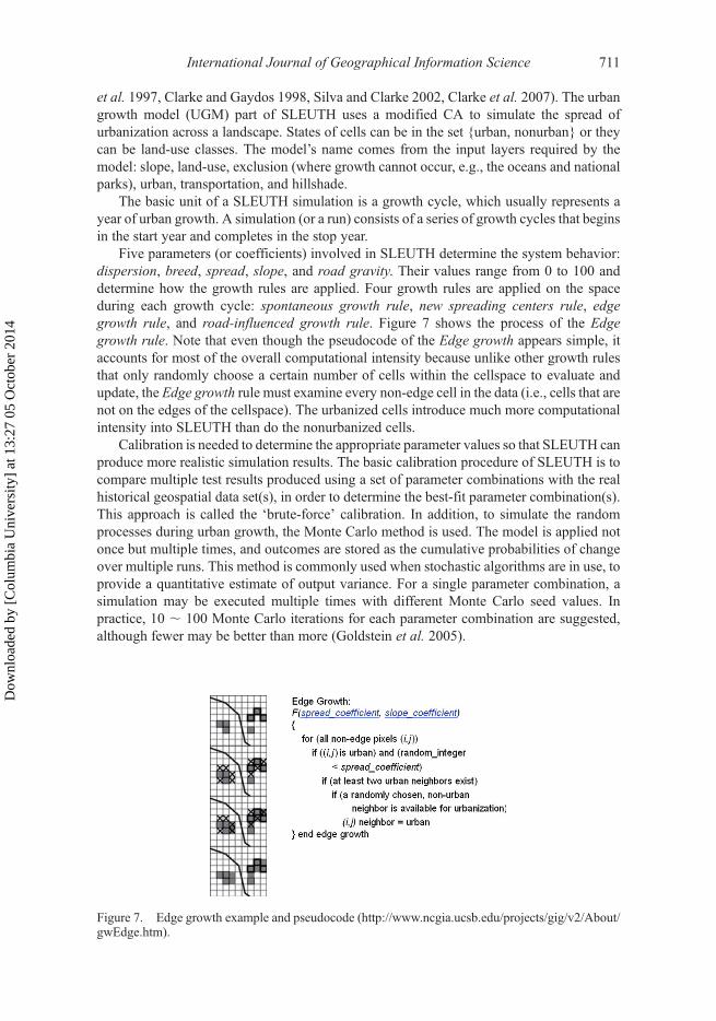
Five parameters (or coefficients) involved in SLEUTH determine the system behavior:dispersion, breed, spread, slope, and road gravity. Their values range from 0 to 100 anddetermine how the growth rules are applied. Four growth rules are applied on the spaceduring each growth cycle: spontaneous growth rule, new spreading centers rule, edgegrowth rule, and road-influenced growth rule. Figure 7 shows the process of the Edgegrowth rule. Note that even though the pseudocode of the Edge growth appears simple, itaccounts for most of the overall computational intensity because unlike other growth rulesthat only randomly choose a certain number of cells within the cellspace to evaluate andupdate, the Edge growth rule must examine every non-edge cell in the data (i.e., cells that arenot on the edges of the cellspace). The urbanized cells introduce much more computationalintensity into SLEUTH than do the nonurbanized cells.

Calibration is needed to determine the appropriate parameter values so that SLEUTH canproduce more realistic simulation results. The basic calibration procedure of SLEUTH is tocompare multiple test results produced using a set of parameter combinations with the realhistorical geospatial data set(s), in order to determine the best-fit parameter combination(s).This approach is called the ‘brute-force’ calibration. In addition, to simulate the randomprocesses during urban growth, the Monte Carlo method is used. The model is applied notonce but multiple times, and outcomes are stored as the cumulative probabilities of changeover multiple runs. This method is commonly used when stochastic algorithms are in use, toprovide a quantitative estimate of output variance. For a single parameter combination, asimulation may be executed multiple times with different Monte Carlo seed values. Inpractice, 10 , 100 Monte Carlo iterations for each parameter combination are suggested,although fewer may be better than more (Goldstein et al. 2005).

Figure 7. Edge growth example and pseudocode (http://www.ncgia.ucsb.edu/projects/gig/v2/About/gwEdge.htm).


Dow

nloa

ded

by [

Col

umbi

a U

nive

rsity

] at

13:

27 0

5 O

ctob

er 2

014

http://www.ncgia.ucsb.edu/projects/gig/v2/About/gwEdge.htm

http://www.ncgia.ucsb.edu/projects/gig/v2/About/gwEdge.htm

All the above together make the calibration process highly computationally intensive. Ina comprehensive (full) calibration, all the possible combinations of the five parameter values(1015 in total) need to be evaluated with multiple Monte Carlo iterations. If 100Monte Carloiterations were used, a comprehensive calibration over a 20-year period would consist of1015 · 100 · 20 growth cycles. Indeed, ‘model calibration for a medium sized data set andminimal data layers requires about 1200 CPU hours on a typical workstation’ (Clarke2003a). This places SLEUTH calibration, especially for large data sets, at the edges ofcomputational tractability.

Apparently, it is infeasible to apply a comprehensive calibration to a relatively largespatial data set with a high resolution over a long time period on a single-processor work-station. A few approaches have been developed to solve this problem. One approach is tomake simplifying assumptions to ignore ‘unimportant’ parameter combinations. The currentSLEUTH model uses this method to seek the best-fit combination, which assumes that theparameters affect the simulation results in a linear manner. However, because of the randomprocesses involved in the CA simulation, the relationships between the parameters and thesimulation results are very likely nonlinear, which makes the calibration results less reliable(Dietzel and Clarke 2007). Another approach is to deploy ‘smart’ algorithms to seek thebest-fit parameter combination(s) without evaluating all the combinations, e.g., the geneticalgorithm (Goldstein 2003) and artificial neural networks (Li and Yeh 2002, Guan et al.2005). This study takes instead a computing-oriented direction, i.e., we deploy parallelcomputing technology to improve the performance of the CA model, hence making itpossible to perform comprehensive calibrations for large spatial data sets over long-termperiods. SLEUTH has been identified as being highly suitable for parallelization, althoughvery little such effort has been conducted to date other than adding MPI routines to thecalibration process to realize a simple task parallelism. The pSLEUTH project takes a stepforward and aims to implement a data–task hybrid parallelism using pRPL.

3.3. Parallelizing SLEUTH using pRPL

pSLEUTH is a parallel version of SLEUTH, developed to improve the performance of theSLEUTH model, especially during the calibration process, by fully utilizing the advancedfeatures of pRPL. More importantly, with the ability to process massive data sets within ashorter period of time, parallel computing is likely to allow the removal of the simplifyingassumptions during the calibration processes. Thus, comprehensive or ‘exhaustive’ calibra-tion processes may produce different best-fit parameter combination(s) other than the one(s)produced by simplified calibration processes, hence altering the final simulation results(Dietzel and Clarke 2007).

The four growth rules of the SLEUTHmodel were implemented using pRPL, such that thedata layers used in the model were decomposed and distributed onto multiple processors.pSLEUTH provides two running modes: FORECAST and CALIBRATE. When running inthe FORECASTmode, a user-defined parameter scenario (which can be the best-fit parametercombination resulting from a calibration process) is given to the program and the sub-cellspaces are processed using the given parameters in parallel on multiple processors. Thefinal forecast result (i.e., the whole cellspace) is gathered to the master processor for an imageoutput (Figure 8). In CALIBRATE mode, a calibration strategy is specified by the user toproduce a set of parameter scenarios, and the sub-cellspaces are processed using the assignedparameters in parallel on a processor group, and the results are compared with the actualhistorical data, which are also decomposed and distributed onto the corresponding processorsto evaluate the simulation performance, i.e., the similarity between the simulated data and the


Dow

nloa

ded

by [

Col

umbi

a U

nive

rsity

] at

13:

27 0

5 O

ctob

er 2

014

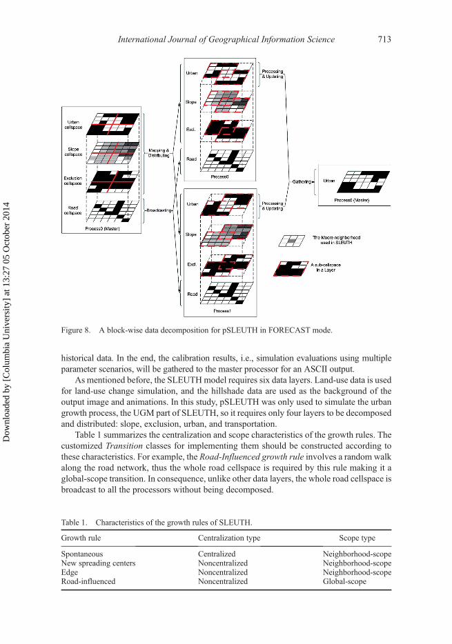
historical data. In the end, the calibration results, i.e., simulation evaluations using multipleparameter scenarios, will be gathered to the master processor for an ASCII output.

As mentioned before, the SLEUTHmodel requires six data layers. Land-use data is usedfor land-use change simulation, and the hillshade data are used as the background of theoutput image and animations. In this study, pSLEUTH was only used to simulate the urbangrowth process, the UGM part of SLEUTH, so it requires only four layers to be decomposedand distributed: slope, exclusion, urban, and transportation.

Table 1 summarizes the centralization and scope characteristics of the growth rules. Thecustomized Transition classes for implementing them should be constructed according tothese characteristics. For example, the Road-Influenced growth rule involves a random walkalong the road network, thus the whole road cellspace is required by this rule making it aglobal-scope transition. In consequence, unlike other data layers, the whole road cellspace isbroadcast to all the processors without being decomposed.

Figure 8. A block-wise data decomposition for pSLEUTH in FORECAST mode.

Table 1. Characteristics of the growth rules of SLEUTH.

Growth rule Centralization type Scope type

Spontaneous Centralized Neighborhood-scopeNew spreading centers Noncentralized Neighborhood-scopeEdge Noncentralized Neighborhood-scopeRoad-influenced Noncentralized Global-scope


Dow

nloa

ded

by [

Col

umbi

a U

nive

rsity

] at

13:

27 0

5 O

ctob

er 2

014

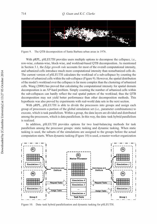
With pRPL, pSLEUTH provides users multiple options to decompose the cellspace, i.e.,row-wise, column-wise, block-wise, and workload-based QTB decomposition. As mentionedin Section 3.1, the Edge growth rule accounts for most of the overall computational intensity,and urbanized cells introduce much more computational intensity than nonurbanized cells do.The current version of pSLEUTH calculates the workload of a sub-cellspace by counting thenumber of urbanized cells within the sub-cellspace (Figure 9). However, the spatial distributionof the model’s workload over the cellspace is far more complex than the clustering of urbanizedcells. Wang (2008) has proved that calculating the computational intensity for spatial domaindecomposition is an NP-hard problem. Simply counting the number of urbanized cells withinthe sub-cellspaces can hardly reflect the real spatial pattern of the workload; thus the QTBdecomposition may not yield better performance than other decomposition methods. Thishypothesis was also proved by experiments with real-world data sets in the next section.

With pRPL, pSLEUTH is able to divide the processors into groups and assign eachgroup of processors a portion of the global simulation set (i.e., parameter combinations) toexecute, which is task parallelism.Within a group, the data layers are divided and distributedamong the processors, which is data parallelism. In this way, the data–task hybrid parallelismis realized.

In addition, pSLEUTH provides options for two load-balancing methods for taskparallelism among the processor groups: static tasking and dynamic tasking. When statictasking is used, the subsets of the simulations are assigned to the groups before the actualcomputation starts. When dynamic tasking (Figure 10) is used, a master-worker organization

Figure 9. The QTB decomposition of Santa Barbara urban areas in 1976.

Figure 10. Data–task hybrid parallelization and dynamic tasking for pSLEUTH.


Dow

nloa

ded

by [

Col

umbi

a U

nive

rsity

] at

13:

27 0

5 O

ctob

er 2

014

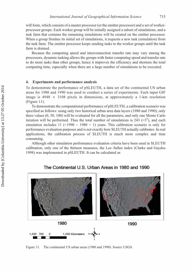
will form, which consists of a master processor (or the emitter processor) and a set of worker-processor groups. Each worker group will be initially assigned a subset of simulations, and atask farm that contains the remaining simulations will be created on the emitter processor.When a group finishes its initial set of simulations, it requests a new task (simulation) fromthe task farm. The emitter processor keeps sending tasks to the worker groups until the taskfarm is drained.

Because the computing speed and interconnection transfer rate may vary among theprocessors, dynamic tasking allows the groups with faster computing speed and transfer rateto do more tasks than other groups, hence it improves the efficiency and shortens the totalcomputing time, especially when there are a large number of simulations to be executed.

4. Experiments and performance analysis

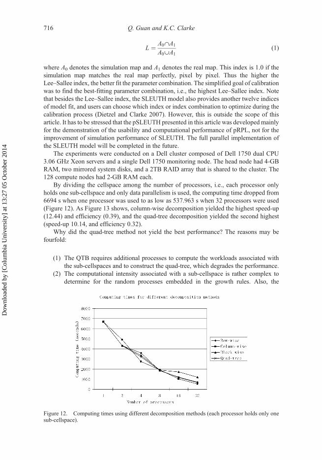
To demonstrate the performance of pSLEUTH, a data set of the continental US urbanareas for 1980 and 1990 was used to conduct a series of experiments. Each input GIFimage is 4948 · 3108 pixels in dimensions, at approximately a 1-km resolution(Figure 11).

To demonstrate the computational performance of pSLEUTH, a calibration scenario wasspecified as follows: using only two historical urban area data layers (1980 and 1990), onlythree values (0, 50, 100) will be evaluated for all the parameters, and only one Monte Carloiteration will be performed. Thus the total number of simulations is 243 (=35), and eachsimulation includes 11 (=1990 - 1980 + 1) years. This calibration scenario is only forperformance evaluation purposes and is not exactly how SLEUTH actually calibrates. In realapplications, the calibration process of SLEUTH is much more complex and timeconsuming.

Although other simulation performance evaluation criteria have been used in SLEUTHcalibration, only one of the thirteen measures, the Lee–Sallee index (Clarke and Gaydos1998) was implemented in pSLEUTH. It can be calculated as

Figure 11. The continental US urban areas (1980 and 1990). Source USGS.


Dow

nloa

ded

by [

Col

umbi

a U

nive

rsity

] at

13:

27 0

5 O

ctob

er 2

014

L ¼ A0˙A1

A0¨A1(1)

where A0 denotes the simulation map and A1 denotes the real map. This index is 1.0 if thesimulation map matches the real map perfectly, pixel by pixel. Thus the higher theLee–Sallee index, the better fit the parameter combination. The simplified goal of calibrationwas to find the best-fitting parameter combination, i.e., the highest Lee–Sallee index. Notethat besides the Lee–Sallee index, the SLEUTH model also provides another twelve indicesof model fit, and users can choose which index or index combination to optimize during thecalibration process (Dietzel and Clarke 2007). However, this is outside the scope of thisarticle. It has to be stressed that the pSLEUTH presented in this article was developed mainlyfor the demonstration of the usability and computational performance of pRPL, not for theimprovement of simulation performance of SLEUTH. The full parallel implementation ofthe SLEUTH model will be completed in the future.

The experiments were conducted on a Dell cluster composed of Dell 1750 dual CPU3.06 GHz Xeon servers and a single Dell 1750 monitoring node. The head node had 4-GBRAM, two mirrored system disks, and a 2TB RAID array that is shared to the cluster. The128 compute nodes had 2-GB RAM each.

By dividing the cellspace among the number of processors, i.e., each processor onlyholds one sub-cellspace and only data parallelism is used, the computing time dropped from6694 s when one processor was used to as low as 537.963 s when 32 processors were used(Figure 12). As Figure 13 shows, column-wise decomposition yielded the highest speed-up(12.44) and efficiency (0.39), and the quad-tree decomposition yielded the second highest(speed-up 10.14, and efficiency 0.32).

Why did the quad-tree method not yield the best performance? The reasons may befourfold:

(1) The QTB requires additional processes to compute the workloads associated withthe sub-cellspaces and to construct the quad-tree, which degrades the performance.

(2) The computational intensity associated with a sub-cellspace is rather complex todetermine for the random processes embedded in the growth rules. Also, the

Figure 12. Computing times using different decomposition methods (each processor holds only onesub-cellspace).


Dow

nloa

ded

by [

Col

umbi

a U

nive

rsity

] at

13:

27 0

5 O

ctob

er 2

014

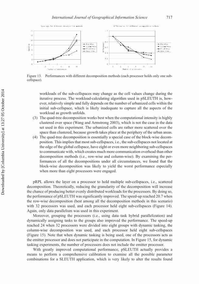
workloads of the sub-cellspaces may change as the cell values change during theiterative process. The workload-calculating algorithm used in pSLEUTH is, how-ever, relatively simple and fully depends on the number of urbanized cells within theinitial sub-cellspace, which is likely inadequate to capture all the aspects of theworkload as growth unfolds.

(3) The quad-tree decomposition works best when the computational intensity is highlyclustered over space (Wang and Armstrong 2003), which is not the case in the dataset used in this experiment. The urbanized cells are rather more scattered over thespace than clustered, because growth takes place at the periphery of the urban areas.

(4) The quad-tree decomposition is essentially a special case of the block-wise decom-position. This implies that most sub-cellspaces, i.e., the sub-cellspaces not located atthe edge of the global cellspace, have eight or even more neighboring sub-cellspacesto communicate with, which creates much more communication overhead than otherdecomposition methods (i.e., row-wise and column-wise). By examining the per-formances of all the decompositions under all circumstances, we found that theblock-wise decomposition was likely to yield the worst performance especiallywhen more than eight processors were engaged.

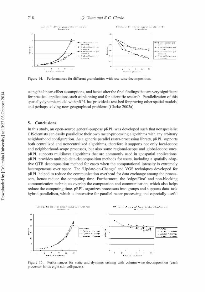
pRPL allows the layer on a processor to hold multiple sub-cellspaces, i.e., scattereddecomposition. Theoretically, reducing the granularity of the decomposition will increasethe chance of producing better evenly distributed workloads for the processors. By doing so,the performance of pSLEUTHwas significantly improved. The speed-up reached 20.7 whenthe row-wise decomposition (best among all the decomposition methods in this scenario)with 32 processors was used, and each processor held eight sub-cellspaces (Figure 14).Again, only data parallelism was used in this experiment.

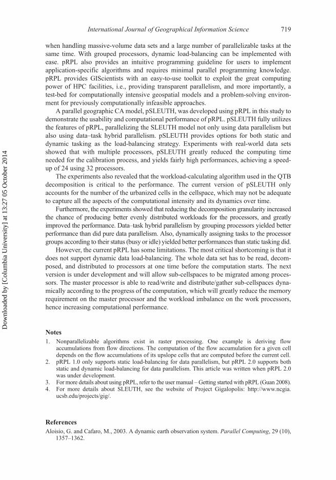
Moreover, grouping the processors (i.e., using data–task hybrid parallelization) anddynamically assigning tasks to the groups also improved the performance. The speed-upreached 24 when 32 processors were divided into eight groups with dynamic tasking, thecolumn-wise decomposition was used, and each processor held eight sub-cellspaces(Figure 15). Note that when dynamic tasking is being used, one of the processors acts asthe emitter processor and does not participate in the computation. In Figure 15, for dynamictasking experiments, the number of processors does not include the emitter processor.

With greatly improved computational performance, pSLEUTH actually provides ameans to perform a comprehensive calibration to examine all the possible parametercombinations for a SLEUTH application, which is very likely to alter the results found

Figure 13. Performances with different decomposition methods (each processor holds only one sub-cellspace).


Dow

nloa

ded

by [

Col

umbi

a U

nive

rsity

] at

13:

27 0

5 O

ctob

er 2

014

using the linear-effect assumptions, and hence alter the final findings that are very significantfor practical applications such as planning and for scientific research. Parallelization of thisspatially dynamicmodel with pRPL has provided a test-bed for proving other spatial models,and perhaps solving new geographical problems (Clarke 2003a).

5. Conclusions

In this study, an open-source general-purpose pRPL was developed such that nonspecialistGIScientists can easily parallelize their own raster-processing algorithms with any arbitraryneighborhood configuration. As a generic parallel raster-processing library, pRPL supportsboth centralized and noncentralized algorithms, therefore it supports not only local-scopeand neighborhood-scope processes, but also some regional-scope and global-scope ones.pRPL supports multilayer algorithms that are commonly used in geospatial applications.pRPL provides multiple data-decomposition methods for users, including a spatially adap-tive QTB decomposition method for cases when the computational intensity is extremelyheterogeneous over space. The ‘Update-on-Change’ and VGS techniques developed forpRPL helped to reduce the communication overhead for data exchange among the proces-sors, hence reduce the computing time. Furthermore, the ‘edgesFirst’ and non-blockingcommunication techniques overlap the computation and communication, which also helpsreduce the computing time. pRPL organizes processors into groups and supports data–taskhybrid parallelism, which is innovative for parallel raster processing and especially useful

Figure 15. Performances for static and dynamic tasking with column-wise decomposition (eachprocessor holds eight sub-cellspaces).

Figure 14. Performances for different granularities with row-wise decomposition.


Dow

nloa

ded

by [

Col

umbi

a U

nive

rsity

] at

13:

27 0

5 O

ctob

er 2

014

when handling massive-volume data sets and a large number of parallelizable tasks at thesame time. With grouped processors, dynamic load-balancing can be implemented withease. pRPL also provides an intuitive programming guideline for users to implementapplication-specific algorithms and requires minimal parallel programming knowledge.pRPL provides GIScientists with an easy-to-use toolkit to exploit the great computingpower of HPC facilities, i.e., providing transparent parallelism, and more importantly, atest-bed for computationally intensive geospatial models and a problem-solving environ-ment for previously computationally infeasible approaches.

A parallel geographic CAmodel, pSLEUTH, was developed using pRPL in this study todemonstrate the usability and computational performance of pRPL. pSLEUTH fully utilizesthe features of pRPL, parallelizing the SLEUTH model not only using data parallelism butalso using data–task hybrid parallelism. pSLEUTH provides options for both static anddynamic tasking as the load-balancing strategy. Experiments with real-world data setsshowed that with multiple processors, pSLEUTH greatly reduced the computing timeneeded for the calibration process, and yields fairly high performances, achieving a speed-up of 24 using 32 processors.

The experiments also revealed that the workload-calculating algorithm used in the QTBdecomposition is critical to the performance. The current version of pSLEUTH onlyaccounts for the number of the urbanized cells in the cellspace, which may not be adequateto capture all the aspects of the computational intensity and its dynamics over time.

Furthermore, the experiments showed that reducing the decomposition granularity increasedthe chance of producing better evenly distributed workloads for the processors, and greatlyimproved the performance. Data–task hybrid parallelism by grouping processors yielded betterperformance than did pure data parallelism. Also, dynamically assigning tasks to the processorgroups according to their status (busy or idle) yielded better performances than static tasking did.

However, the current pRPL has some limitations. The most critical shortcoming is that itdoes not support dynamic data load-balancing. The whole data set has to be read, decom-posed, and distributed to processors at one time before the computation starts. The nextversion is under development and will allow sub-cellspaces to be migrated among proces-sors. The master processor is able to read/write and distribute/gather sub-cellspaces dyna-mically according to the progress of the computation, which will greatly reduce the memoryrequirement on the master processor and the workload imbalance on the work processors,hence increasing computational performance.

Notes

1. Nonparallelizable algorithms exist in raster processing. One example is deriving flowaccumulations from flow directions. The computation of the flow accumulation for a given celldepends on the flow accumulations of its upslope cells that are computed before the current cell.

2. pRPL 1.0 only supports static load-balancing for data parallelism, but pRPL 2.0 supports bothstatic and dynamic load-balancing for data parallelism. This article was written when pRPL 2.0was under development.

3. For more details about using pRPL, refer to the user manual – Getting started with pRPL (Guan 2008).4. For more details about SLEUTH, see the website of Project Gigalopolis: http://www.ncgia.

ucsb.edu/projects/gig/.

ReferencesAloisio, G. and Cafaro, M., 2003. A dynamic earth observation system. Parallel Computing, 29 (10),

1357–1362.


Dow

nloa

ded

by [

Col

umbi

a U

nive

rsity

] at

13:

27 0

5 O

ctob

er 2

014

http://www.ncgia.ucsb.edu/projects/gig/

http://www.ncgia.ucsb.edu/projects/gig/

Ananthanarayan, A., et al., 2003. Data webs for earth science data. Parallel Computing, 29 (10),1363–1379.

Armstrong, M.P., 2000. Geography and computational science. Annals of the Association of AmericanGeographers, 90 (1), 146–168.

Armstrong, M.P. and Marciano, R., 1993. Parallel spatial interpolation. In: Proceedings of the eleventhinternational symposium on computer-assisted cartography (Auto-Carto 11). Bethesda, MD:American Congress on Surveying and Mapping, 414–423.

Armstrong, M.P. and Marciano, R., 1995. Massively parallel processing of spatial statistics.International Journal of Geographical Information Science, 9 (2), 169–189.

Armstrong, M.P. and Marciano, R.J., 1996. Local interpolation using a distributed parallel super-computer. International Journal of Geographical Information Systems, 10 (6), 713–729.

Armstrong, M.P. and Marciano, R.J., 1997. Massively parallel strategies for local spatial interpolation.Computers and Geosciences, 23 (8), 859–867.

Bandini, S., Mauri, G., and Serra, R., 2001. Cellular automata: from a theoretical parallel computa-tional model to its application to complex systems. Parallel Computing, 27, 539–553.

Batty, M., 2000. GeoComputation using cellular automata. In: S. Openshaw and R.J. Abrahart, eds.GeoComputation. New York, NY: Taylor & Francis, 95–126.

Benjamin, S.C., Johnson, N.F. and Hui, P.M., 1996. Cellular automata models of traffic flow along ahighway containing a junction. Journal of Physics A: Mathematical and General, 29 (12),3119–3127.

Bhattacharya, P., 2001. Efficient neighbor finding algorithms in quadtree and octree. M.T. Thesis.Dept. Comp. Science and Eng., India Inst. Technology, Kanpur.

Cannan, E., 2001. The origin of the law of diminishing returns, 1813–1815. Available from: http://socserv.mcmaster.ca/,econ/ugcm/3ll3/cannan/cannan003.html [Accessed 12 August 2008].

Cannataro, M., et al., 1995. A parallel cellular automata environment on multicomputers for computa-tional science. Parallel Computing, 21 (5), 803–823.

Clarke, K.C., 1995. Analytical and computer cartography. Englewood Cliffs, NJ: Prentice Hall.Clarke, K.C., 2003a. Geocomputation’s future at the extremes: high performance computing and

nanoclients. Parallel Computing, 29 (10), 1281–1295.Clarke, K.C., 2003b. Getting started with geographic information systems. Upper Saddle River, NJ:

Pearson Education.Clarke, K.C. and Gaydos, L.J., 1998. Loose-coupling a cellular automaton model and GIS: long-term

urban growth prediction for San Francisco and Washington/Baltimore. International Journal ofGeographical Information Science, 12 (7), 699–714.

Clarke, K.C., Hoppen, S., and Gaydos, L., 1997. A Self-modifying cellular automaton model ofhistorical urbanization in the San Francisco Bay Area. Environment and Planning B: Planningand Design, 24 (2), 247–261.

Clarke, K.C., Riggan, P., and Brass, J.A., 1995. A cellular automaton model of wildfire propagationand extinction. Photogrammetric Engineering and Remote Sensing, 60 (11), 1355–1367.

Clarke, K.C. et al., 2007. A decade of SLEUTHing: lessons learned from applications of a cellularautomaton land use change model. In: P. Fisher, ed. Classics from IJGIS. Twenty years of theinternational journal of geographical information systems and science. Boca Raton, FL: Taylorand Francis, CRC, 413–425.

Clematis, A., Mineter, M., and Marciano, R., 2003. High performance computing with geographicaldata. Parallel Computing, 29 (10), 1275–1279.

Cosnard, M. and Trystram, D., 1995. Parallel algorithms and architecture, Boston, MA: InternationalThomson Computer Press.

Couclelis, H., 1997. From cellular automata to urban models: new principles for model developmentand implementation. Environment and planning B: planning and design, 24 (2), 165–174.

Cramer, B.E. and Armstrong, M.P., 1997. Interpolation of spatially inhomogeneous data sets: anevaluation of parallel computation approaches. In: Proceedings of GIS/LIS’97. Bethesda, MD:American Congress on Surveying and Mapping.

Dietzel, C. and Clarke, K.C., 2007. Toward optimal calibration of the SLEUTH land use change model.Transactions in GIS, 11 (1), 29–45.

Ding, Y. and Densham, P.J., 1996. Spatial strategies for parallel spatial modelling. InternationalJournal of Geographical Information Systems, 10 (6), 669–698.

Duckham, M., Goodchild, M.F. and Worboys, M.F., 2003. Foundations of geographic informationscience. New York: Taylor & Francis.


Dow

nloa

ded

by [

Col

umbi

a U

nive

rsity

] at

13:

27 0

5 O

ctob

er 2

014

http://socserv.mcmaster.ca/,econ/ugcm/3ll3/cannan/cannan003.html

http://socserv.mcmaster.ca/,econ/ugcm/3ll3/cannan/cannan003.html

Goldstein, N.C., Dietzel, C., and Clarke, K.C., 2005. Don’t stop ‘til you get enough–sensitivity testingofMonte Carlo iterations for model calibration. InProceedings of the 8th International Conferenceon GeoComputation, Ann Arbor, MI..

Goldstein, N.C., 2003. Brains vs Braun – comparative strategies for the calibration of a cellularautomata-based urban growth model. In: Proceedings of the 7th international conference onGeoComputation, Southampton, England..

Gropp, W., et al., 1998. MPI: the complete reference (Vol. 2), Cambridge, MA: The MIT Press.Guan, Q., 2008. Getting started with pRPL. Available from: http://www.geog.ucsb.edu/,guan/pRPL/

Getting_started_with_pRPL.pdf.Guan, Q., Wang, L., and Clarke, K., 2005. An artificial-neural-network-based, constrained CA model

for simulating urban growth. Cartography and Geographic Information Science, 32 (4), 369–380.Harris, B., 1985. Some notes on parallel computing: with special reference to transportation and land-

use modeling. Environment and Planning A, 17 (9), 1275–1278.Healey, S., et al., eds., 1998. Parallel processing algorithms for GIS. Bristol, PA: Taylor & Francis.Hecker, C., et al., 1999. System development for parallel cellular automata and its applications. Future

Generation Computing Systems, 16 (2–3), 235–247.Hutchinson, D. et al., 1996. Parallel Neighboourhood Modelling. In: Proceedings of the 4th ACM

international workshop on advances in geographic information systems. Rockville, MD,25–34.

Kerry, K.E. and Hawick, K.A., 1997. Spatial interpolation on distributed, high-performance compu-ters. Technical Report DHPC-015. Department of Computer Science, University of Adelaide.

Kerry, K.E. and Hawick, K.A., 1998. Kriging interpolation on high-performance computers. In:Proceedings of the international conference and exhibition on high-performance computing andnetworking. Amsterdam: Springer-Verlag, 429–438.

Kidner, D.B., Rallings, P.J. and Ware, J.A., 1997. Parallel processing for terrain analysis in GIS:visibility as a case study. GeoInformatica, 1 (2), 183–207.

Li, B., 1992. Opportunities and challenges of parallel spatial data analysis: initial experiments with dataparallel map analysis. In: GIS LIS-international conference, . San Jose, 445–458..

Li, X. and Yeh, A.G.O., 2000. Modelling sustainable urban development by the integration ofconstrained cellular automata and GIS. International Journal of Geographical InformationScience, 14 (2): 131–152.

Li, X. and Yeh, A.G.O., 2002. Neural-network-based cellular automata for simulating multiple land usechanges using GIS. International Journal of Geographical Information Science, 16 (4), 323–343.

Lloyd, C.D., 2007. Local models for spatial analysis. Boca Raton, FL, USA: CRC Press.Mineter, M.J., 1998. Partitioning raster data. In: R.D. Healey, et al., eds. Parallel processing

algorithms for GIS. Bristol, PA: Taylor & Francis, 215–230.Mineter, M.J. and Dowers, S., 1999. Parallel processing for geographical applications: a layered

approach. Journal of Geographical Systems, 1 (1), 61–74.Montanvert, A., Meer, P., and Rosenfeld, A., 1991. Hierarchical image analysis using irregular

tessellations. IEEE transactions on pattern analysis and machine intelligence, 13 (4), 307–316.Nagel, K. and Schreckenberg, M., 1992. A cellular automaton model for freeway traffic. Journal of

Physics I France, 2, 2221–2229.Nieplocha, J. et al., 2007. Global arrays user manual. Available from: http://www.emsl.pnl.gov/docs/

global/um/GA.pdf [Accessed 11 August 2008].Openshaw, S. and Turton, I., 2000.High performance computing and the art of parallel programming:

an introduction for geographers, social scientists, and engineers. New York, NY: Routledge.O’Sullivan, D., 2001. Graph-cellular automata: a generalised discrete urban and regional model.

Environment and Planning B: Planning and Design, 28 (5), 687–705.Peucker, T.K. and Douglas, D.H., 1975. Detection of surface-specific points by local parallel proces-

sing of discrete terrain elevation data. Computer Graphics and Image Processing, 4, 375–387.Puppo, E., et al., 1994. Parallel terrain triangulation. International Journal of Geographical

Information Science, 8 (2), 105–128.Rokos, D. and Armstrong, M.P., 1992. Parallel terrain feature extraction. In: Proceedings of GIS/LIS

‘92. Bethesda, MD: American Congress on Surveying and Mapping, 652–661.Saalfeld, A., 2000. Complexity and intractability: limitations to implementation in analytical carto-

graphy. Cartography and GIS, 27 (3), 239–249.Samet, H., 1982. Neighbor finding techniques for images represented by quadtrees. Computer

Graphics and Image Processing, 18 (1), 37–57.


Dow

nloa

ded

by [

Col

umbi

a U

nive

rsity

] at

13:

27 0

5 O

ctob

er 2

014

http://www.geog.ucsb.edu/~guan/pRPL/Getting_started_with_pRPL.pdf.

http://www.geog.ucsb.edu/~guan/pRPL/Getting_started_with_pRPL.pdf.

http://www.emsl.pnl.gov/docs/global/um/GA.pdf

http://www.emsl.pnl.gov/docs/global/um/GA.pdf

Samet, H., 1984. The quadtree and related hierarchical data structures. ACM Computing Surveys, 16(2), 187–260.

Samet, H., 1990. Applications of spatial data structures: Computer graphics, image processing, andGIS. Reading, MA: Addison-Wesley Longman Publishing Co., Inc.

Sandu, J.S. and Marble, D.F., 1988. An investigation into the utility of the cray X-MP supercomputerfor handling spatial data. In: Proceedings of the third international symposium on spatial datahandling. Sydney, Australia, 253–266.

Silva, E.A. and Clarke, K.C., 2002. Calibration of the SLEUTH urban growth model for Lisbon andPorto. Computers, Environment and Urban Systems, 26 (6), 525–552.

Smith, T.R., Gao, P. and Gahinet, P., 1989. Asynchronous, iterative, and parallel procedures for solvingthe weighted-region least cost path problem. Geographical Analysis, 21 (2), 147–166.

Spezzano, G. and Talia, D., 1999. Programming cellular automata algorithms on parallel computers.Future Generation Computing Systems, 16 (2), 203–216.

Spezzano, G. et al., 1996. A parallel cellular tool for interactive modeling and simulation. IEEEComputational Science and Engineering, 3 (3), 33–43.

Tomlin, C.D., 1990. Geographic information systems and cartographic modelling. Englewood Cliffs,NJ: Prentice-Hall.

Wang, F., 1993. A parallel intersection algorithm for vector polygon overlay. IEEE Computer Graphicsand Applications, 13 (2), 74–81.

Wang, S., 2008. Formalizing computational intensity of spatial analysis. In: Proceedings of the 5thinternational conference on geographic information science, , 23–26, September 2008. ParkCity, UT.

Wang, S. and Armstrong, M.P., 2003. A quadtree approach to domain decomposition for spatialinterpolation in grid computing environments. Parallel Computing, 29 (10), 1481–1504.

White, R., Engelen, G. and Uljee, I., 1997. The use of constrained cellular automata for high-resolutionmodelling of urban land-use dynamics. Environment and Planning B: Planning and Design, 24(3), 323–343.

Worboys, M. and Duckham, M., 2004. GIS: a computing perspective. New York: CRC Press.Wu, F. and Webster, C.J., 1998. Simulation of land development through the integration of cellular

automata and multi-criteria evaluation. Environment and Planning B, 25 (1), 103–126.Yeh, A.G.O. and Li, X., 2001. A constrained CA model for the simulation and planning of sustainable

urban forms by using GIS. Environment and Planning B: Planning and Design, 28 (5), 733–753.Yeh, A.G.O. and Li, X., 2002. Urban simulation using neural networks and cellular automata for land

use planning. In: D. Richardson and P.V. Oosterom, eds. Advances in spatial data handling. AnnArbor, MI: The University of Michigan Press, 451–464.


Dow

nloa

ded

by [

Col

umbi

a U

nive

rsity

] at

13:

27 0

5 O

ctob

er 2

014

Documents

A general-purpose parallel raster processing programming library test application using a geographic cellular automata model