A Fistful of Dollars:Formalizing Asymptotic Complexity Claims

via Deductive Program Verification

Armael Gueneau1, Arthur Chargueraud1,2, and Francois Pottier1?

1 Inria2 Universite de Strasbourg, CNRS, ICube UMR 7357

Abstract. We present a framework for simultaneously verifying thefunctional correctness and the worst-case asymptotic time complexityof higher-order imperative programs. We build on top of SeparationLogic with Time Credits, embedded in an interactive proof assistant.We formalize the O notation, which is key to enabling modular specifi-cations and proofs. We cover the subtleties of the multivariate case, wherethe complexity of a program fragment depends on multiple parameters.We propose a way of integrating complexity bounds into specifications,present lemmas and tactics that support a natural reasoning style, andillustrate their use with a collection of examples.

1 Introduction

A program or program component whose functional correctness has been verifiedmight nevertheless still contain complexity bugs: that is, its performance, in somescenarios, could be much poorer than expected.

Indeed, many program verification tools only guarantee partial correctness,that is, do not even guarantee termination, so a verified program could runforever. Some program verification tools do enforce termination, but usuallydo not allow establishing an explicit complexity bound. Tools for automaticcomplexity inference can produce complexity bounds, but usually have limitedexpressive power.

In practice, many complexity bugs are revealed by testing. Some have alsobeen detected during ordinary program verification, as shown by Filliatre andLetouzey [14], who find a violation of the balancing invariant in a widely-distributed implementation of binary search trees. Nevertheless, none of thesetechniques can guarantee, with a high degree of assurance, the absence of com-plexity bugs in software.

To illustrate the issue, consider the binary search implementation in Figure 1.Virtually every modern software verification tool allows proving that this OCamlcode (or analogous code, expressed in another programming language) satisfiesthe specification of a binary search and terminates on all valid inputs. This code

? This research was partly supported by the French National Research Agency (ANR)under the grant ANR-15-CE25-0008.

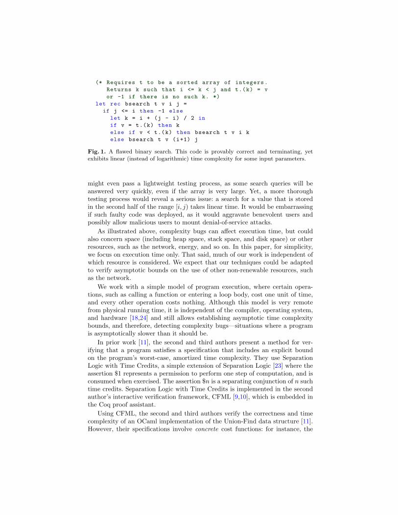
(* Requires t to be a sorted array of integers.

Returns k such that i <= k < j and t.(k) = v

or -1 if there is no such k. *)

let rec bsearch t v i j =

if j <= i then -1 else

let k = i + (j - i) / 2 in

if v = t.(k) then k

else if v < t.(k) then bsearch t v i k

else bsearch t v (i+1) j

Fig. 1. A flawed binary search. This code is provably correct and terminating, yetexhibits linear (instead of logarithmic) time complexity for some input parameters.

might even pass a lightweight testing process, as some search queries will beanswered very quickly, even if the array is very large. Yet, a more thoroughtesting process would reveal a serious issue: a search for a value that is storedin the second half of the range [i, j) takes linear time. It would be embarrassingif such faulty code was deployed, as it would aggravate benevolent users andpossibly allow malicious users to mount denial-of-service attacks.

As illustrated above, complexity bugs can affect execution time, but couldalso concern space (including heap space, stack space, and disk space) or otherresources, such as the network, energy, and so on. In this paper, for simplicity,we focus on execution time only. That said, much of our work is independent ofwhich resource is considered. We expect that our techniques could be adaptedto verify asymptotic bounds on the use of other non-renewable resources, suchas the network.

We work with a simple model of program execution, where certain opera-tions, such as calling a function or entering a loop body, cost one unit of time,and every other operation costs nothing. Although this model is very remotefrom physical running time, it is independent of the compiler, operating system,and hardware [18,24] and still allows establishing asymptotic time complexitybounds, and therefore, detecting complexity bugs—situations where a programis asymptotically slower than it should be.

In prior work [11], the second and third authors present a method for ver-ifying that a program satisfies a specification that includes an explicit boundon the program’s worst-case, amortized time complexity. They use SeparationLogic with Time Credits, a simple extension of Separation Logic [23] where theassertion $1 represents a permission to perform one step of computation, and isconsumed when exercised. The assertion $n is a separating conjunction of n suchtime credits. Separation Logic with Time Credits is implemented in the secondauthor’s interactive verification framework, CFML [9,10], which is embedded inthe Coq proof assistant.

Using CFML, the second and third authors verify the correctness and timecomplexity of an OCaml implementation of the Union-Find data structure [11].However, their specifications involve concrete cost functions: for instance, the

precondition of the function find indicates that calling find requires and con-sumes $(2α(n) + 4), where n is the current number of elements in the datastructure, and where α denotes an inverse of Ackermann’s function. We wouldprefer the specification to give the asymptotic complexity bound O(α(n)), whichmeans that, for some function f ∈ O(α(n)), calling find requires and consumes$f(n). This is the purpose of this paper.

We argue that the use of asymptotic bounds, such as O(α(n)), is necessaryfor (verified or unverified) complexity analysis to be applicable at scale. At asuperficial level, it reduces clutter in specifications and proofs: O(mn) is morecompact and readable than 3mn+ 2n log n+ 5n+ 3m+ 2. At a deeper level, it iscrucial for stating modular specifications, which hide the details of a particularimplementation. Exposing the fact that find costs 2α(n) + 4 is undesirable: ifa tiny modification of the Union-Find module changes this cost to 2α(n) + 5,then all direct and indirect clients of the Union-Find module must be updated,which is intolerable. Furthermore, sometimes, the constant factors are unknownanyway. Applying the Master Theorem [12] to a recurrence equation only yieldsan order of growth, not a concrete bound. Finally, for most practical purposes, nocritical information is lost when concrete bounds such as 2α(n) + 4 are replacedwith asymptotic bounds such as O(α(n)). Indeed, the number of computationsteps that take place at the source level is related to physical time only upto a hardware- and compiler-dependent constant factor. The use of asymptoticcomplexity in the analysis of algorithms, initially advocated by Hopcroft and byTarjan, has been widely successful and is nowadays standard practice.

One must be aware of several limitations of our approach. First, it is not aworst-case execution time (WCET) analysis: it does not yield bounds on actualphysical execution time. Second, it is not fully automated. We place emphasison expressiveness, as opposed to automation. Our vision is that verifying thefunctional correctness and time complexity of a program, at the same time,should not involve much more effort than verifying correctness alone. Third,we control only the growth of the cost as the parameters grow large. A loopthat counts up from 0 to 260 has complexity O(1), even though it typicallywon’t terminate in a lifetime. Although this is admittedly a potential problem,traditional program verification falls prey to analogous pitfalls: for instance, aprogram that attempts to allocate and initialize an array of size (say) 248 can beproved correct, even though, on contemporary desktop hardware, it will typicallyfail by lack of memory. We believe that there is value in our approach in spiteof these limitations.

Reasoning and working with asymptotic complexity bounds is not as simpleas one might hope. As demonstrated by several examples in §2, typical paperproofs using the O notation rely on informal reasoning principles which can easilybe abused to prove a contradiction. Of course, using a proof assistant steers usclear of this danger, but implies that our proofs cannot be quite as simple andperhaps cannot have quite the same structure as their paper counterparts.

A key issue that we run against is the handling of existential quantifiers.According to what was said earlier, the specification of a sorting algorithm, say

mergesort, should be, roughly: “there exists a cost function f ∈ O(λn.n log n)such that mergesort is content with $f(n), where n is the length of the inputlist.” Therefore, the very first step in a naıve proof of mergesort must be toexhibit a witness for f , that is, a concrete cost function. An appropriate witnessmight be λn.2n log n, or λn.n log n + 3, who knows? This information is notavailable up front, at the very beginning of the proof; it becomes available onlyduring the proof, as we examine the code of mergesort, step by step. It is notreasonable to expect the human user to guess such a witness. Instead, it seemsdesirable to delay the production of the witness and to gradually construct a costexpression as the proof progresses. In the case of a nonrecursive function, suchas insertionsort, the cost expression, once fully synthesized, yields the desiredwitness. In the case of a recursive function, such as mergesort, the cost expressionyields the body of a recurrence equation, whose solution is the desired witness.

We make the following contributions:

1. We formalize the O notation as a binary domination relation between func-tions of type A → Z, where the type A is chosen by the user. Functionsof several variables are covered by instantiating A with a product type. Wecontend that, in order to define what it means for a ∈ A to “grow large”, or“tend towards infinity”, the type A must be equipped with a filter [6], thatis, a quantifier Ua.P . We propose a library of lemmas and tactics that canprove nonnegativeness, monotonicity, and domination assertions (§3).

2. We propose a standard style of writing specifications, in the setting of theCFML program verification framework, so that they integrate asymptotictime complexity claims (§4). We define a predicate, specO, which imposesthis style and incorporates a few important technical decisions, such as thefact that every cost function must be nonnegative and nondecreasing.

3. We propose a methodology, supported by a collection of Coq tactics, to provesuch specifications (§5). Our tactics, which heavily rely on Coq metavari-ables, help gradually synthesize cost expressions for straight-line code andconditionals, and help construct the recurrence equations involved in theanalysis of recursive functions, while delaying their resolution.

4. We present several classic examples of complexity analyses (§6), including:a simple loop in O(n.2n), nested loops in O(n3) and O(nm), binary searchin O(log n), and Union-Find in O(α(n)).

Our code can be found online in the form of two standalone Coq librariesand a self-contained archive [16].

2 Challenges in Reasoning with the O Notation

When informally reasoning about the complexity of a function, or of a codeblock, it is customary to make assertions of the form “this code has asymptoticcomplexity O(1)”, “that code has asymptotic complexity O(n)”, and so on. Yet,these assertions are too informal: they do not have sufficiently precise meaning,and can be easily abused to produce flawed paper proofs.

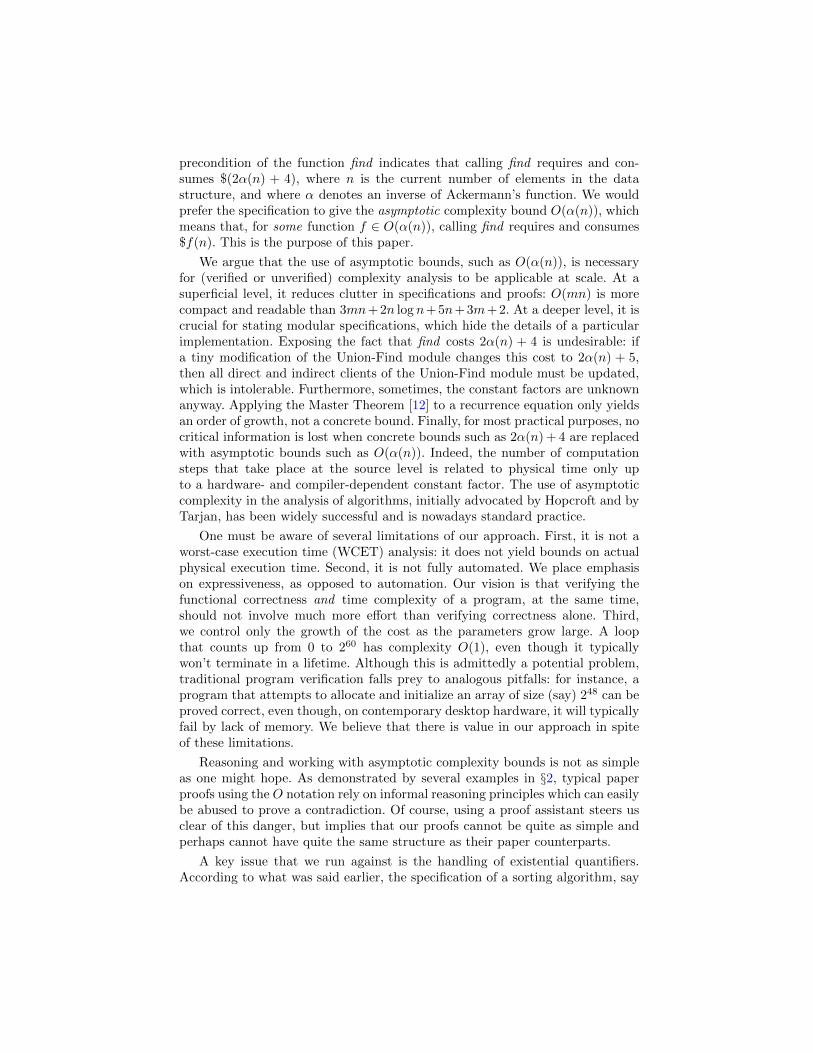
Incorrect claim: The OCaml function waste has asymptotic complexity O(1).

let rec waste n =

if n > 0 then waste (n-1)

Flawed proof:Let us prove by induction on n that waste(n) costs O(1).

– Case n ≤ 0: waste(n) terminates immediately. Therefore, its cost is O(1).

– Case n > 0: A call to waste(n) involves constant-time processing, followed with acall to waste(n− 1). By the induction hypothesis, the cost of the recursive call isO(1). We conclude that the cost of waste(n) is O(1) +O(1), that is, O(1).

Fig. 2. A flawed proof that waste(n) costs O(1), when its actual cost is O(n).

Incorrect claim: The OCaml function f has asymptotic complexity O(1).

let g (n, m) =

for i = 1 to n do

for j = 1 to m do () done

done

let f n = g (n, 0)

Flawed proof:

– g(n,m) involves nm inner loop iterations, thus costs O(nm).

– The cost of f(n) is the cost of g(n, 0), plus O(1). As the cost of g(n,m) is O(nm),we find, by substituting 0 for m, that the cost of g(n, 0) is O(0). Thus, f(n) is O(1).

Fig. 3. A flawed proof that f(n) costs O(1), when its actual cost is O(n).

A striking example appears in Figure 2, which shows how one might “prove”that a recursive function has complexity O(1), whereas its actual cost is O(n).The flawed proof exploits the (valid) relation O(1) +O(1) = O(1), which meansthat a sequence of two constant-time code fragments is itself a constant-timecode fragment. The flaw lies in the fact that the O notation hides an existentialquantification, which is inadvertently swapped with the universal quantificationover the parameter n. Indeed, the claim is that “there exists a constant c suchthat, for every n, waste(n) runs in at most c computation steps”. However,the proposed proof by induction establishes a much weaker result, to wit: “forevery n, there exists a constant c such that waste(n) runs in at most c steps”.This result is certainly true, yet does not entail the claim.

An example of a different nature appears in Figure 3. There, the auxiliaryfunction g takes two integer arguments n and m and involves two nested loops,over the intervals [1, n] and [1,m]. Its asymptotic complexity is O(n+nm), which,under the hypothesis that m is large enough, can be simplified to O(nm). Thereasoning, thus far, is correct. The flaw lies in our attempt to substitute 0 for min the bound O(nm). Because this bound is valid only for sufficiently large m, itdoes not make sense to substitute a specific value for m. In other words, from thefact that “g(n,m) costs O(nm) when n and m are sufficiently large”, one cannot

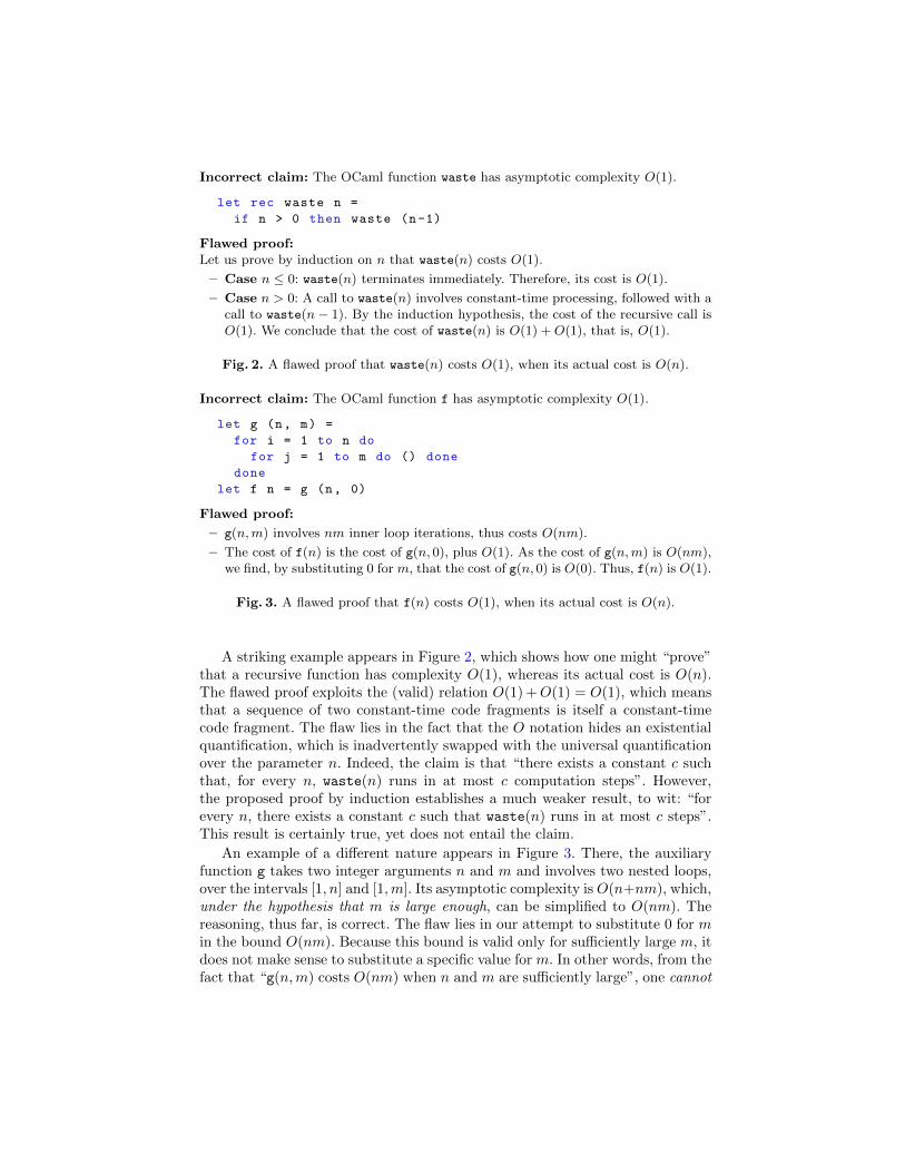
Incorrect claim: The OCaml function h has asymptotic complexity O(nm2).

1 for i = 0 to m−1 do

2 let p = ( if i = 0 then pow2 n else n∗i ) in

3 for j = 1 to p do ( ) done

4 done

Flawed proof:

– The body of the outer loop (lines 3-4) has asymptotic cost O(ni). Indeed, as soonas i > 0 holds, the inner loop performs ni constant-time iterations. The case wherei = 0 does not matter in an asymptotic analysis.

– The cost of h(m,n) is the sum of the costs of the iterations of the outer loop:∑m−1i=0 O(ni) = O

(n ·∑m−1

i=0 i)

= O(nm2).

Fig. 4. A flawed proof that h(m,n) costs O(nm2), when its actual cost is O(2n +nm2).

deduce anything about the cost of g(n, 0). To repair this proof, one must takea step back and prove that g(n,m) has asymptotic complexity O(n + nm) forsufficiently large n and for every m. This fact can be instantiated with m = 0,allowing one to correctly conclude that g(n, 0) costs O(n). We come back to thisexample in §3.3.

One last example of tempting yet invalid reasoning appears in Figure 4. Weborrow it from Howell [19]. This flawed proof exploits the dubious idea that “theasymptotic cost of a loop is the sum of the asymptotic costs of its iterations”. Inmore precise terms, the proof relies on the following implication, where f(m,n, i)represents the true cost of the i-th loop iteration and g(m,n, i) represents anasymptotic bound on f(m,n, i):

f(m,n, i) ∈ O(g(m,n, i)) ⇒∑m−1

i=0 f(m,n, i) ∈ O(∑m−1

i=0 g(m,n, i))

As pointed out by Howell, this implication is in fact invalid. Here, f(m,n, 0) is 2n

and f(m,n, i) when i > 0 is ni, while g(m,n, i) is just ni. The left-hand side of

the above implication holds, but the right-hand side does not, as 2n +∑m−1

i=1 niis O(2n + nm2), not O(nm2). The Summation lemma presented later on in thispaper (Lemma 8) rules out the problem by adding the requirement that f be anondecreasing function of the loop index i. We discuss in depth later on (§4.5)why cost functions should and can be monotonic.

The examples that we have presented show that the informal reasoning styleof paper proofs, where the O notation is used in a loose manner, is unsound.One cannot hope, in a formal setting, to faithfully mimic this reasoning style. Inthis paper, we do assign O specifications to functions, because we believe thatthis style is elegant, modular and scalable. However, during the analysis of afunction body, we abandon the O notation. We first synthesize a cost expressionfor the function body, then check that this expression is indeed dominated bythe asymptotic bound that appears in the specification.

3 Formalizing the O Notation

3.1 Domination

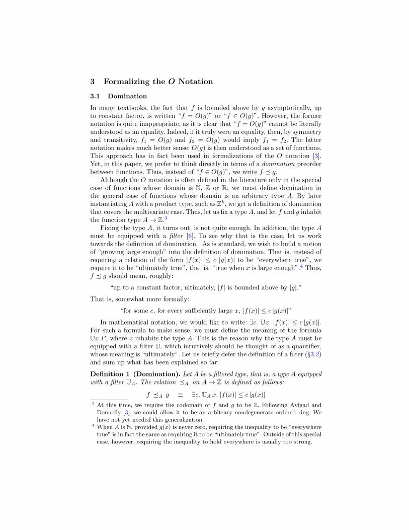
In many textbooks, the fact that f is bounded above by g asymptotically, upto constant factor, is written “f = O(g)” or “f ∈ O(g)”. However, the formernotation is quite inappropriate, as it is clear that “f = O(g)” cannot be literallyunderstood as an equality. Indeed, if it truly were an equality, then, by symmetryand transitivity, f1 = O(g) and f2 = O(g) would imply f1 = f2. The latternotation makes much better sense: O(g) is then understood as a set of functions.This approach has in fact been used in formalizations of the O notation [3].Yet, in this paper, we prefer to think directly in terms of a domination preorderbetween functions. Thus, instead of “f ∈ O(g)”, we write f � g.

Although the O notation is often defined in the literature only in the specialcase of functions whose domain is N, Z or R, we must define domination inthe general case of functions whose domain is an arbitrary type A. By laterinstantiating A with a product type, such as Zk, we get a definition of dominationthat covers the multivariate case. Thus, let us fix a type A, and let f and g inhabitthe function type A→ Z.3

Fixing the type A, it turns out, is not quite enough. In addition, the type Amust be equipped with a filter [6]. To see why that is the case, let us worktowards the definition of domination. As is standard, we wish to build a notionof “growing large enough” into the definition of domination. That is, instead ofrequiring a relation of the form |f(x)| ≤ c |g(x)| to be “everywhere true”, werequire it to be “ultimately true”, that is, “true when x is large enough”.4 Thus,f � g should mean, roughly:

“up to a constant factor, ultimately, |f | is bounded above by |g|.”

That is, somewhat more formally:

“for some c, for every sufficiently large x, |f(x)| ≤ c |g(x)|”

In mathematical notation, we would like to write: ∃c. Ux. |f(x)| ≤ c |g(x)|.For such a formula to make sense, we must define the meaning of the formulaUx.P , where x inhabits the type A. This is the reason why the type A must beequipped with a filter U, which intuitively should be thought of as a quantifier,whose meaning is “ultimately”. Let us briefly defer the definition of a filter (§3.2)and sum up what has been explained so far:

Definition 1 (Domination). Let A be a filtered type, that is, a type A equippedwith a filter UA. The relation �A on A→ Z is defined as follows:

f �A g ≡ ∃c. UA x. |f(x)| ≤ c |g(x)|3 At this time, we require the codomain of f and g to be Z. Following Avigad and

Donnelly [3], we could allow it to be an arbitrary nondegenerate ordered ring. Wehave not yet needed this generalization.

4 When A is N, provided g(x) is never zero, requiring the inequality to be “everywheretrue” is in fact the same as requiring it to be “ultimately true”. Outside of this specialcase, however, requiring the inequality to hold everywhere is usually too strong.

3.2 Filters

Whereas ∀x.P means that P holds of every x, and ∃x.P means that P holdsof some x, the formula Ux.P should be taken to mean that P holds of everysufficiently large x, that is, P ultimately holds.

The formula Ux.P is short for U (λx.P ). If x ranges over some type A, thenU must have type P(P(A)), where P(A) is short for A → Prop. To stress thisbetter, although Bourbaki [6] states that a filter is “a set of subsets of A”, it iscrucial to note that P(P(A)) is the type of a quantifier in higher-order logic.

Definition 2 (Filter). A filter [6] on a type A is an object U of type P(P(A))that enjoys the following four properties, where Ux.P is short for U (λx.P ):

(1) (P1 ⇒ P2)⇒ Ux.P1 ⇒ Ux.P2 (covariance)(2a) Ux.P1 ∧ Ux.P2 ⇒ Ux.(P1 ∧ P2) (stability under binary intersection)(2b) Ux.True (stability under 0-ary intersection)(3) Ux.P ⇒ ∃x.P (nonemptiness)

Properties (1)–(3) are intended to ensure that the intuitive reading of Ux.Pas: “for sufficiently large x, P holds” makes sense. Property (1) states that ifP1 implies P2 and if P1 holds when x is large enough, then P2, too, shouldhold when x is large enough. Properties (2a) and (2b), together, state that ifeach of P1, . . . , Pk independently holds when x is large enough, then P1, . . . , Pk

should simultaneously hold when x is large enough. Properties (1) and (2b)together imply ∀x.P ⇒ Ux.P . Property (3) states that if P holds when x is largeenough, then P should hold of some x. In classical logic, it would be equivalentto ¬(Ux.False).

In the following, we let the metavariable A stand for a filtered type, that is, apair of a carrier type and a filter on this type. By abuse of notation, we also writeA for the carrier type. (In Coq, this is permitted by an implicit projection.) Wewrite UA for the filter.

3.3 Examples of Filters

When U is a universal filter, Ux.Q(x) is (by definition) equivalent to ∀x.Q(x).Thus, a predicate Q is “ultimately true” if and only if it is “everywhere true”.In other words, the universal quantifier is a filter.

Definition 3 (Universal filter). Let T be a nonempty type. Then λQ.∀x.Q(x)is a filter on T .

When U is the order filter associated with the ordering ≤, the formulaUx.Q(x) means that, when x becomes sufficiently large with respect to ≤, theproperty Q(x) becomes true.

Definition 4 (Order filter). Let (T,≤) be a nonempty ordered type, such thatevery two elements have an upper bound. Then λQ.∃x0.∀x ≥ x0. Q(x) is a filteron T .

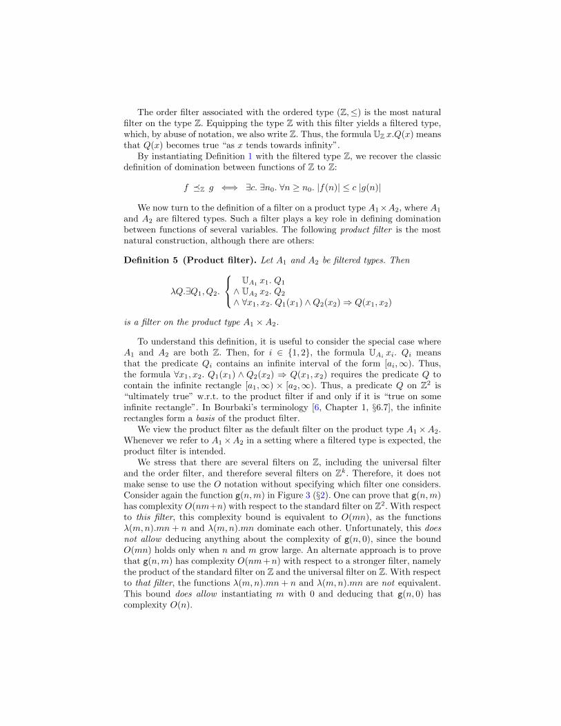
The order filter associated with the ordered type (Z,≤) is the most naturalfilter on the type Z. Equipping the type Z with this filter yields a filtered type,which, by abuse of notation, we also write Z. Thus, the formula UZ x.Q(x) meansthat Q(x) becomes true “as x tends towards infinity”.

By instantiating Definition 1 with the filtered type Z, we recover the classicdefinition of domination between functions of Z to Z:

f �Z g ⇐⇒ ∃c. ∃n0. ∀n ≥ n0. |f(n)| ≤ c |g(n)|

We now turn to the definition of a filter on a product type A1×A2, where A1

and A2 are filtered types. Such a filter plays a key role in defining dominationbetween functions of several variables. The following product filter is the mostnatural construction, although there are others:

Definition 5 (Product filter). Let A1 and A2 be filtered types. Then

λQ.∃Q1, Q2.

UA1 x1. Q1

∧ UA2 x2. Q2

∧ ∀x1, x2. Q1(x1) ∧Q2(x2)⇒ Q(x1, x2)

is a filter on the product type A1 ×A2.

To understand this definition, it is useful to consider the special case whereA1 and A2 are both Z. Then, for i ∈ {1, 2}, the formula UAi

xi. Qi meansthat the predicate Qi contains an infinite interval of the form [ai,∞). Thus,the formula ∀x1, x2. Q1(x1) ∧ Q2(x2) ⇒ Q(x1, x2) requires the predicate Q tocontain the infinite rectangle [a1,∞) × [a2,∞). Thus, a predicate Q on Z2 is“ultimately true” w.r.t. to the product filter if and only if it is “true on someinfinite rectangle”. In Bourbaki’s terminology [6, Chapter 1, §6.7], the infiniterectangles form a basis of the product filter.

We view the product filter as the default filter on the product type A1×A2.Whenever we refer to A1×A2 in a setting where a filtered type is expected, theproduct filter is intended.

We stress that there are several filters on Z, including the universal filterand the order filter, and therefore several filters on Zk. Therefore, it does notmake sense to use the O notation without specifying which filter one considers.Consider again the function g(n,m) in Figure 3 (§2). One can prove that g(n,m)has complexity O(nm+n) with respect to the standard filter on Z2. With respectto this filter, this complexity bound is equivalent to O(mn), as the functionsλ(m,n).mn + n and λ(m,n).mn dominate each other. Unfortunately, this doesnot allow deducing anything about the complexity of g(n, 0), since the boundO(mn) holds only when n and m grow large. An alternate approach is to provethat g(n,m) has complexity O(nm+n) with respect to a stronger filter, namelythe product of the standard filter on Z and the universal filter on Z. With respectto that filter, the functions λ(m,n).mn+ n and λ(m,n).mn are not equivalent.This bound does allow instantiating m with 0 and deducing that g(n, 0) hascomplexity O(n).

3.4 Properties of Domination

Many properties of the domination relation can be established with respect to anarbitrary filtered type A. Here are two example lemmas; there are many more.As before, f and g range over A → Z. The operators f + g, max(f, g) and f.gdenote pointwise sum, maximum, and product, respectively.

Lemma 6 (Sum and Max Are Alike). Assume f and g are ultimately non-negative, that is, UA x. f(x) ≥ 0 and UA x. g(x) ≥ 0 hold. Then, we havemax(f, g) �A f + g and f + g �A max(f, g).

Lemma 7 (Multiplication). f1 �A g1 and f2 �A g2 imply f1.f2 �A g1.g2.

Lemma 7 corresponds to Howell’s Property 5 [19]. Whereas Howell states thisproperty on Nk, our lemma is polymorphic in the type A. As noted by Howell,this lemma is useful when the cost of a loop body is independent of the loopindex. In the case where the cost of the i-th iteration may depend on the loopindex i, the following, more complex lemma is typically used instead:

Lemma 8 (Summation). Let f, g range over A → Z → Z. Let i0 ∈ Z.Assume the following three properties:

1. UA a. ∀i ≥ i0. f(a)(i) ≥ 0.2. UA a. ∀i ≥ i0. g(a)(i) ≥ 0.3. for every a, the function λi.f(a)(i) is nondecreasing on the interval [i0,∞).

Then,λ(a, i).f(a)(i) �A×Z λ(a, i).g(a)(i)

impliesλ(a, n).

∑ni=i0

f(a)(i) �A×Z λ(a, n).∑n

i=i0g(a)(i).

Lemma 8 uses the product filter on A × Z in its hypothesis and conclusion.It corresponds to Howell’s property 2 [19]. The variable i represents the loopindex, while the variable a collectively represents all other variables in scope, sothe type A is usually instantiated with a tuple type (an example appears in §6).

An important property is the fact that function composition is compatible,in a certain sense, with domination. This allows transforming the parametersunder which an asymptotic analysis is carried out (examples appear in §6). Dueto space limitations, we refer the reader to the Coq library for details [16].

3.5 Tactics

Our formalization of filters and domination forms a stand-alone Coq library [16].In addition to many lemmas about these notions, the library proposes automatedtactics that can prove nonnegativeness, monotonicity, and domination goals.These tactics currently support functions built out of variables, constants, sumsand maxima, products, powers, logarithms. Extending their coverage is ongoingwork. This library is not tied to our application to the complexity analysis ofprograms. It could have other applications in mathematics.

4 Specifications with Asymptotic Complexity Claims

In this section, we first present our existing approach to verified time complexityanalysis. This approach, proposed by the second and third authors [11], does notuse the O notation: instead, it involves explicit cost functions. We then discusshow to extend this approach with support for asymptotic complexity claims. Wefind that, even once domination (§3) is well-understood, there remain nontrivialquestions as to the style in which program specifications should be written. Wepropose one style which works well on small examples and which we believeshould scale well to larger ones.

4.1 CFML With Time Credits For Cost Analysis

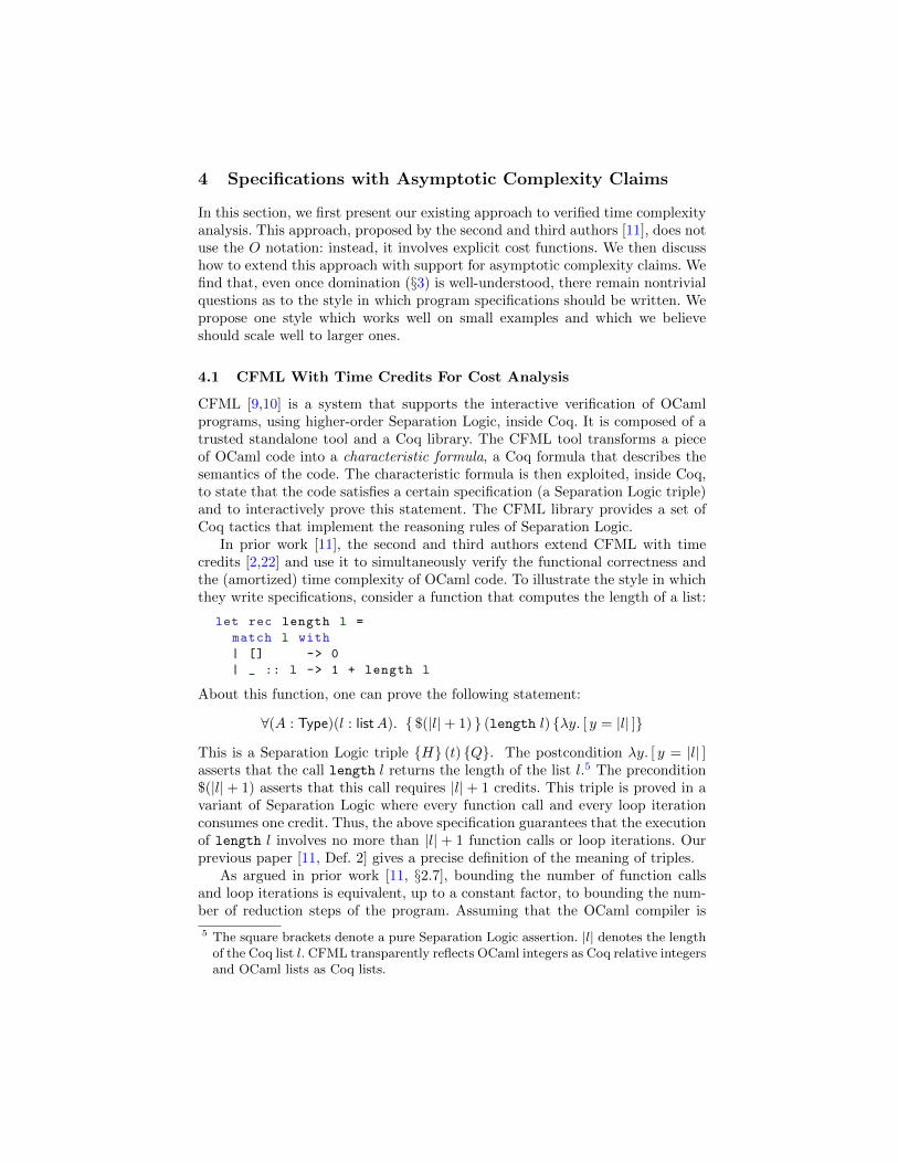
CFML [9,10] is a system that supports the interactive verification of OCamlprograms, using higher-order Separation Logic, inside Coq. It is composed of atrusted standalone tool and a Coq library. The CFML tool transforms a pieceof OCaml code into a characteristic formula, a Coq formula that describes thesemantics of the code. The characteristic formula is then exploited, inside Coq,to state that the code satisfies a certain specification (a Separation Logic triple)and to interactively prove this statement. The CFML library provides a set ofCoq tactics that implement the reasoning rules of Separation Logic.

In prior work [11], the second and third authors extend CFML with timecredits [2,22] and use it to simultaneously verify the functional correctness andthe (amortized) time complexity of OCaml code. To illustrate the style in whichthey write specifications, consider a function that computes the length of a list:

let rec length l =

match l with

| [] -> 0

| _ :: l -> 1 + length l

About this function, one can prove the following statement:

∀(A : Type)(l : listA). { $(|l|+ 1) } (length l) {λy. [ y = |l| ]}

This is a Separation Logic triple {H} (t) {Q}. The postcondition λy. [ y = |l| ]asserts that the call length l returns the length of the list l.5 The precondition$(|l|+ 1) asserts that this call requires |l|+ 1 credits. This triple is proved in avariant of Separation Logic where every function call and every loop iterationconsumes one credit. Thus, the above specification guarantees that the executionof length l involves no more than |l| + 1 function calls or loop iterations. Ourprevious paper [11, Def. 2] gives a precise definition of the meaning of triples.

As argued in prior work [11, §2.7], bounding the number of function callsand loop iterations is equivalent, up to a constant factor, to bounding the num-ber of reduction steps of the program. Assuming that the OCaml compiler is

5 The square brackets denote a pure Separation Logic assertion. |l| denotes the lengthof the Coq list l. CFML transparently reflects OCaml integers as Coq relative integersand OCaml lists as Coq lists.

complexity-preserving, this is equivalent, up to a constant factor, to boundingthe number of instructions executed by the compiled code. Finally, assumingthat the machine executes one instruction in bounded time, this is equivalent,up to a constant factor, to bounding the execution time of the compiled code.Thus, the above specification guarantees that length runs in linear time.

Instead of understanding Separation Logic with Time Credits as a variantof Separation Logic, one can equivalently view it as standard Separation Logic,applied to an instrumented program, where a pay() instruction has been in-serted at the beginning of every function body and loop body. The proof of theprogram is carried out under the axiom {$1} (pay()) {λ .>}, which imposes theconsumption of one time credit at every pay() instruction. This instruction hasno runtime effect: it is just a way of marking where credits must be consumed.

For example, the OCaml function length is instrumented as follows:

let rec length l =

pay();

match l with [] -> 0 | _ :: l -> 1 + length l

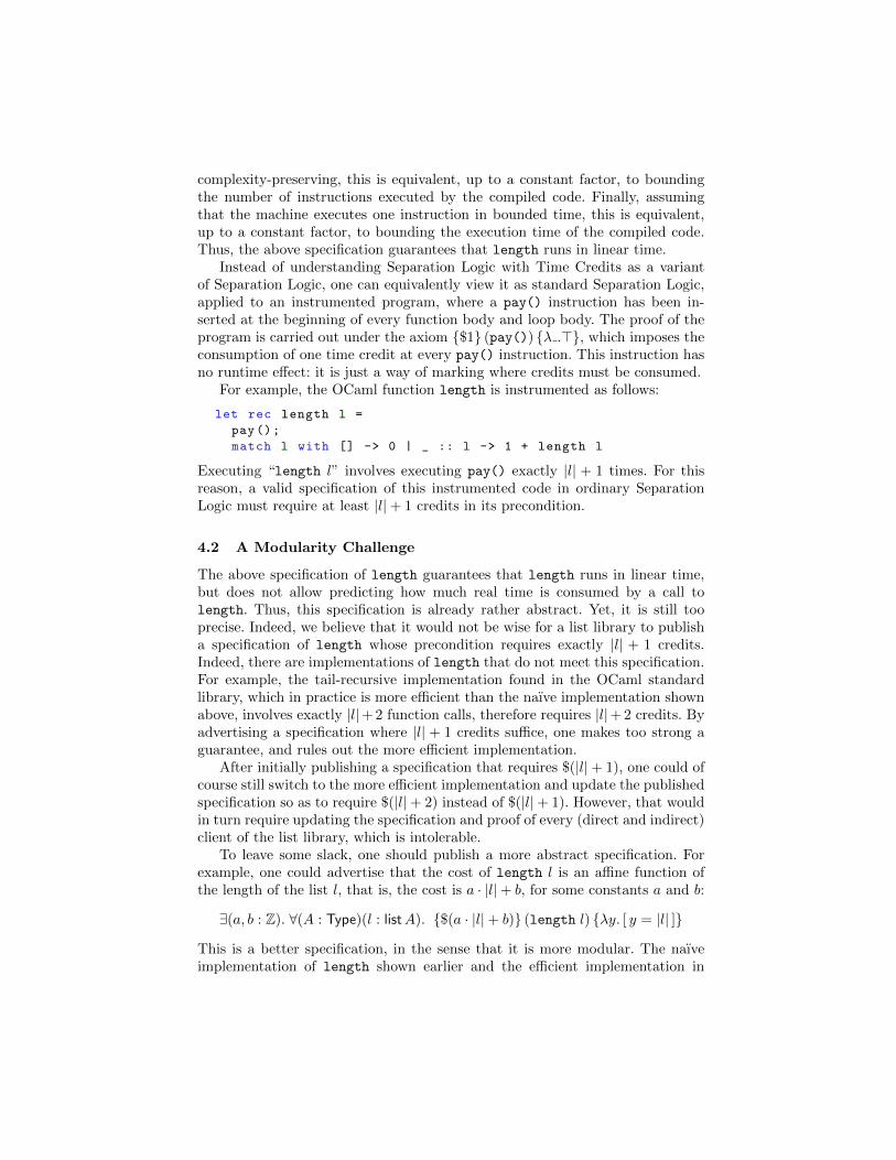
Executing “length l” involves executing pay() exactly |l| + 1 times. For thisreason, a valid specification of this instrumented code in ordinary SeparationLogic must require at least |l|+ 1 credits in its precondition.

4.2 A Modularity Challenge

The above specification of length guarantees that length runs in linear time,but does not allow predicting how much real time is consumed by a call tolength. Thus, this specification is already rather abstract. Yet, it is still tooprecise. Indeed, we believe that it would not be wise for a list library to publisha specification of length whose precondition requires exactly |l| + 1 credits.Indeed, there are implementations of length that do not meet this specification.For example, the tail-recursive implementation found in the OCaml standardlibrary, which in practice is more efficient than the naıve implementation shownabove, involves exactly |l|+ 2 function calls, therefore requires |l|+ 2 credits. Byadvertising a specification where |l| + 1 credits suffice, one makes too strong aguarantee, and rules out the more efficient implementation.

After initially publishing a specification that requires $(|l|+ 1), one could ofcourse still switch to the more efficient implementation and update the publishedspecification so as to require $(|l|+ 2) instead of $(|l|+ 1). However, that wouldin turn require updating the specification and proof of every (direct and indirect)client of the list library, which is intolerable.

To leave some slack, one should publish a more abstract specification. Forexample, one could advertise that the cost of length l is an affine function ofthe length of the list l, that is, the cost is a · |l|+ b, for some constants a and b:

∃(a, b : Z). ∀(A : Type)(l : listA). {$(a · |l|+ b)} (length l) {λy. [ y = |l| ]}

This is a better specification, in the sense that it is more modular. The naıveimplementation of length shown earlier and the efficient implementation in

OCaml’s standard library both satisfy this specification, so one is free to chooseone or the other, without any impact on the clients of the list library. In fact,any reasonable implementation of length should have linear time complexityand therefore should satisfy this specification.

That said, the style in which the above specification is written is arguablyslightly too low-level. Instead of directly expressing the idea that the cost oflength l is O(|l|), we have written this cost under the form a · |l| + b. It ispreferable to state at a more abstract level that cost is dominated by λn.n: sucha style is more readable and scales to situations where multiple parameters andnonstandard filters are involved. Thus, we propose the following statement:

∃cost : Z→ Z.{

cost �Z λn. n∀(A : Type)(l : listA). {$cost(|l|)} (length l) {λy. [ y = |l| ]}

Thereafter, we refer to the function cost as the concrete cost of length, asopposed to the asymptotic bound, represented here by the function λn. n. Thisspecification asserts that there exists a concrete cost function cost , which isdominated by λn. n, such that cost(|l|) credits suffice to justify the executionof length l. Thus, cost(|l|) is an upper bound on the actual number of pay()instructions that are executed at runtime.

The above specification informally means that length l has time complexityO(n) where the parameter n represents |l|, that is, the length of the list l. Thefact that n represents |l| is expressed by applying cost to |l| in the precondition.The fact that this analysis is valid when n grows large enough is expressed byusing the standard filter on Z in the assertion cost �Z λn. n.

In general, it is up to the user to choose what the parameters of the costanalysis should be, what these parameters represent, and which filter on theseparameters should be used. The example of the Bellman-Ford algorithm (§6)illustrates this.

4.3 A Record For Specifications

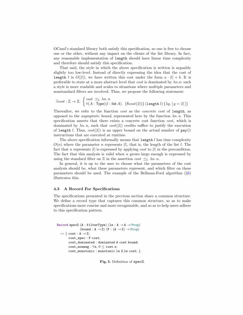
The specifications presented in the previous section share a common structure.We define a record type that captures this common structure, so as to makespecifications more concise and more recognizable, and so as to help users adhereto this specification pattern.

Record specO (A : filterType) (le : A → A → Prop)(bound : A → Z) (P : (A → Z) → Prop)

:= { cost : A → Z;cost_spec : P cost;cost_dominated : dominated A cost bound;cost_nonneg : ∀x, 0 ≤ cost x;cost_monotonic : monotonic le Z.le cost; }.

Fig. 5. Definition of specO.

This type, specO, is defined in Figure 5. The first three fields in this recordtype correspond to what has been explained so far. The first field asserts theexistence of a function cost of A to Z, where A is a user-specified filtered type.The second field asserts that a certain property P cost is satisfied; it is typically aSeparation Logic triple whose precondition refers to cost. The third field assertsthat cost is dominated by the user-specified function bound. The need for thelast two fields is explained further on (§4.4, §4.5).

Using this definition, our proposed specification of length (§4.2) is stated inconcrete Coq syntax as follows:

Theorem length_spec:specO Z_filterType Z.le (fun n ⇒ n) (fun cost ⇒∀A (l:list A), triple (length l)PRE ($ (cost |l|))POST (fun y ⇒ [ y = |l| ]))

The key elements of this specification are Z_filterType, which is Z, equippedwith its standard filter; the asymptotic bound fun n ⇒ n, which means thatthe time complexity of length is O(n); and the Separation Logic triple, whichdescribes the behavior of length, and refers to the concrete cost function cost.

One key technical point is that specO is a strong existential, whose witnesscan be referred to via to the first projection, cost. For instance, the concretecost function associated with length can be referred to as cost length_spec.Thus, at a call site of the form length xs, the number of required credits iscost length_spec |xs|.

In the next subsections, we explain why, in the definition of specO, we requirethe concrete cost function to be nonnegative and monotonic. These are designdecisions; although these properties may not be strictly necessary, we find thatenforcing them greatly simplifies things in practice.

4.4 Why Cost Functions Must Be Nonnegative

There are several common occasions where one is faced with the obligation ofproving that a cost expression is nonnegative. These proof obligations arise fromseveral sources.

One source is the Separation Logic axiom for splitting credits, whose state-ment is $(m+ n) = $m ? $n, subject to the side conditions m ≥ 0 and n ≥ 0.Without these side conditions, out of $0, one would be able to create $1 ? $(−1).Because our logic is affine, one could then discard $(−1), keeping just $1. Inshort, an unrestricted splitting axiom would allow creating credits out of thinair.6 Another source of proof obligations is the Summation lemma (Lemma 8),which requires the functions at hand to be (ultimately) nonnegative.

6 Another approach would be to define $n only for n ∈ N, in which case an unrestrictedaxiom would be sound. However, as we use Z everywhere, that would be inconvenient.A more promising idea is to view $n as linear (as opposed to affine) when n isnegative. Then, $(−1) cannot be discarded, so unrestricted splitting is sound.

Now, suppose one is faced with the obligation of proving that the expressioncost length_spec |xs| is nonnegative. Because length_spec is an existentialpackage (a specO record), this is impossible, unless this information has beenrecorded up front within the record. This is the reason why the field cost_nonneg

in Figure 5 is needed.For simplicity, we require cost functions to be nonnegative everywhere, as

opposed to within a certain domain. This requirement is stronger than neces-sary, but simplifies things, and can easily be met in practice by wrapping costfunctions within “max(0,−)”. Our Coq tactics automatically insert “max(0,−)”wrappers where necessary, making this issue mostly transparent to the user. Inthe following, for brevity, we write c+ for max(0, c), where c ∈ Z.

4.5 Why Cost Functions Must Be Monotonic

One key reason why cost functions should be monotonic has to do with the“avoidance problem”. When the cost of a code fragment depends on a localvariable x, can this cost be reformulated (and possibly approximated) in sucha way that the dependency is removed? Indeed, a cost expression that makessense outside the scope of x is ultimately required.

The problematic cost expression is typically of the form E[|x|], where |x|represents some notion of the “size” of the data structure denoted by x, and E isan arithmetic context, that is, an arithmetic expression with a hole. Furthermore,an upper bound on |x| is typically available. This upper bound can be exploitedif the context E is monotonic, i.e., if x ≤ y implies E[x] ≤ E[y]. Because thehole in E can appear as an actual argument to an abstract cost function, wemust record the fact that this cost function is monotonic.

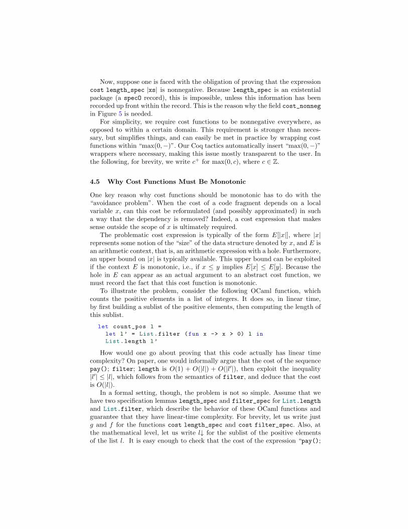
To illustrate the problem, consider the following OCaml function, whichcounts the positive elements in a list of integers. It does so, in linear time,by first building a sublist of the positive elements, then computing the length ofthis sublist.

let count_pos l =

let l’ = List.filter (fun x -> x > 0) l in

List.length l’

How would one go about proving that this code actually has linear timecomplexity? On paper, one would informally argue that the cost of the sequencepay(); filter; length is O(1) + O(|l|) + O(|l′|), then exploit the inequality|l′| ≤ |l|, which follows from the semantics of filter, and deduce that the costis O(|l|).

In a formal setting, though, the problem is not so simple. Assume that wehave two specification lemmas length_spec and filter_spec for List.lengthand List.filter, which describe the behavior of these OCaml functions andguarantee that they have linear-time complexity. For brevity, let us write justg and f for the functions cost length_spec and cost filter_spec. Also, atthe mathematical level, let us write l↓ for the sublist of the positive elementsof the list l. It is easy enough to check that the cost of the expression “pay();

let l’ = ... in List.length l’” is 1 + f(|l|) + g(|l′|). The problem, now, isto find an upper bound for this cost that does not depend on l′, a local variable,and to verify that this upper bound, expressed as a function of |l|, is dominatedby λn. n. Indeed, this is required in order to establish a specO statement aboutcount_pos.

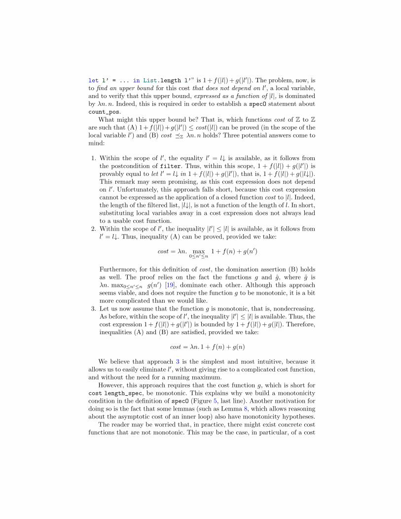
What might this upper bound be? That is, which functions cost of Z to Zare such that (A) 1+f(|l|)+g(|l′|) ≤ cost(|l|) can be proved (in the scope of thelocal variable l′) and (B) cost �Z λn. n holds? Three potential answers come tomind:

1. Within the scope of l′, the equality l′ = l↓ is available, as it follows fromthe postcondition of filter. Thus, within this scope, 1 + f(|l|) + g(|l′|) isprovably equal to let l′ = l↓ in 1 + f(|l|) + g(|l′|), that is, 1 + f(|l|) + g(|l↓|).This remark may seem promising, as this cost expression does not dependon l′. Unfortunately, this approach falls short, because this cost expressioncannot be expressed as the application of a closed function cost to |l|. Indeed,the length of the filtered list, |l↓|, is not a function of the length of l. In short,substituting local variables away in a cost expression does not always leadto a usable cost function.

2. Within the scope of l′, the inequality |l′| ≤ |l| is available, as it follows froml′ = l↓. Thus, inequality (A) can be proved, provided we take:

cost = λn. max0≤n′≤n

1 + f(n) + g(n′)

Furthermore, for this definition of cost , the domination assertion (B) holdsas well. The proof relies on the fact the functions g and g, where g isλn. max0≤n′≤n g(n′) [19], dominate each other. Although this approachseems viable, and does not require the function g to be monotonic, it is a bitmore complicated than we would like.

3. Let us now assume that the function g is monotonic, that is, nondecreasing.As before, within the scope of l′, the inequality |l′| ≤ |l| is available. Thus, thecost expression 1 + f(|l|) + g(|l′|) is bounded by 1 + f(|l|) + g(|l|). Therefore,inequalities (A) and (B) are satisfied, provided we take:

cost = λn. 1 + f(n) + g(n)

We believe that approach 3 is the simplest and most intuitive, because itallows us to easily eliminate l′, without giving rise to a complicated cost function,and without the need for a running maximum.

However, this approach requires that the cost function g, which is short forcost length_spec, be monotonic. This explains why we build a monotonicitycondition in the definition of specO (Figure 5, last line). Another motivation fordoing so is the fact that some lemmas (such as Lemma 8, which allows reasoningabout the asymptotic cost of an inner loop) also have monotonicity hypotheses.

The reader may be worried that, in practice, there might exist concrete costfunctions that are not monotonic. This may be the case, in particular, of a cost

function f that is obtained as the solution of a recurrence equation. Fortunately,in the common case of functions of Z to Z, the “running maximum” function fcan always be used in place of f : indeed, it is monotonic and has the sameasymptotic behavior as f . Thus, we see that both approaches 2 and 3 aboveinvolve running maxima in some places, but their use seems less frequent withapproach 3.

5 Interactive Proofs of Asymptotic Complexity Claims

To prove a specification lemma, such as length_spec (§4.3) or loop_spec (§4.4),one must construct a specO record. By definition of specO (Figure 5), this meansthat one must exhibit a concrete cost function cost and prove a number of prop-erties of this function, including the fact that, when supplied with $(cost . . .),the code runs correctly (cost_spec) and the fact that cost is dominated by thedesired asymptotic bound (cost_dominated).

Thus, the very first step in a naıve proof attempt would be to guess anappropriate cost function for the code at hand. However, such an approach wouldbe painful, error-prone, and brittle. It seems much preferable, if possible, to enlistthe machine’s help in synthesizing a cost function at the same time as we stepthrough the code—which we have to do anyway, as we must build a SeparationLogic proof of the correctness of this code.

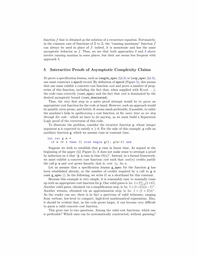
To illustrate the problem, consider the recursive function p, whose integerargument n is expected to satisfy n ≥ 0. For the sake of this example, p calls anauxiliary function g, which we assume runs in constant time.

let rec p n =

if n <= 1 then () else begin g(); p(n-1) end

Suppose we wish to establish that p runs in linear time. As argued at thebeginning of the paper (§2, Figure 2), it does not make sense to attempt a proofby induction on n that “p n runs in time O(n)”. Instead, in a formal framework,we must exhibit a concrete cost function cost such that cost(n) credits justifythe call p n and cost grows linearly, that is, cost �Z λn. n.

Let us assume that a specification lemma g_spec for the function g hasbeen established already, so the number of credits required by a call to g iscost g_spec (). In the following, we write G as a shorthand for this constant.

Because this example is very simple, it is reasonably easy to manually comeup with an appropriate cost function for p. One valid guess is λn. 1+Σn

i=2(1+G).Another valid guess, obtained via a simplification step, is λn. 1+(1+G)(n−1)+.Another witness, obtained via an approximation step, is λn. 1 + (1 + G)n+.As the reader can see, there is in fact a spectrum of valid witnesses, rangingfrom verbose, low-level to compact, high-level mathematical expressions. Also,it should be evident that, as the code grows larger, it can become very difficultto guess a valid concrete cost function.

This gives rise to two questions. Among the valid cost functions, which oneis preferable? Which ones can be systematically constructed, without guessing?

Among the valid cost functions, there is a tradeoff. At one extreme, a low-levelcost function has exactly the same syntactic structure as the code, so it is easy toprove that it is an upper bound for the actual cost of the code, but a lot of workmay be involved in proving that it is dominated by the desired asymptotic bound.At the other extreme, a high-level cost function can be essentially identical to thedesired asymptotic bound, up to explicit multiplicative and additive constants,so the desired domination assertion is trivial, but a lot of accounting work maybe involved in proving that this function represents enough credits to executethe code. Thus, by choosing a cost function, we shift some of the burden of theproof from one subgoal to another. From this point of view, no cost functionseems inherently preferable to another.

From the point of view of systematic construction, however, the answer ismore clear-cut. It seems fairly clear that it is possible to systematically build acost function whose syntactic structure is the same as the syntactic structure ofthe code. This idea goes at least as far back as Wegbreit’s work [26]. Coming upwith a compact, high-level expression of the cost, on the other hand, seems torequire human insight.

To provide as much machine assistance as possible, our system mechanicallysynthesizes a low-level cost expression for a piece of OCaml code. This is donetransparently, at the same time as the user constructs a proof of the code inSeparation Logic. Furthermore, we take advantage of the fact that we are usingan interactive proof assistant: we allow the user to guide the synthesis process.For instance, the user controls how a local variable should be eliminated, how thecost of a conditional construct should be approximated (i.e., by a conditional orby a maximum), and how recurrence equations should be solved. In the following,we present this semi-interactive synthesis process. We first consider straight-line(nonrecursive) code (§5.1), then recursive functions (§5.2).

5.1 Synthesizing Cost Expressions For Straight-Line Code

The CFML library provides the user with interactive tactics that implement thereasoning rules of Separation Logic. We set things up in such a way that, asthese rules are applied, a cost expression is automatically synthesized.

To this end, we use specialized variants of the reasoning rules, whose premisesand conclusions take the form {$n ? H} (e) {Q}. Furthermore, to simplify thenonnegativeness side conditions that must be proved while reasoning, we make allcost expressions obviously nonnegative by wrapping them in max(0,−). Recallthat c+ stands for max(0, c), where c ∈ Z. Our reasoning rules work with triplesof the form {$ c+ ? H} (e) {Q}. They are shown in Figure 6.

Because we wish to synthesize a cost expression, our Coq tactics maintainthe following invariant: whenever the goal is {$ c+ ? H} (e) {Q}, the cost c isuninstantiated, that is, it is represented in Coq by a metavariable, a placeholder.This metavariable is instantiated when the goal is proved by applying one ofthe reasoning rules. Such an application produces new subgoals, whose precon-ditions contain new metavariables. As this process is repeated, a cost expressionis incrementally constructed.

WeakenCost{$ c+2 ? H} (e) {Q} c+2 ≤ c1

{$ c1 ? H} (e) {Q}

Seq

{$ c+1 ? H} (e1) {Q′} {$ c+2 ? Q′()} (e2) {Q}

{$ (c+1 + c+2 )+ ? H} (e1; e2) {Q}

Let{$ c+1 ? H} (e1) {Q′} ∀x. {$ c+2 ? Q

′(x)} (e2) {Q}{$ (c+1 + c+2 )+ ? H} (let x = e1 in e2) {Q}

ValH Q(v)

{$ 0+ ? H} (v) {Q}

Ifb = true⇒ {$ c+1 ? H} (e1) {Q}b = false⇒ {$ c+2 ? H} (e2) {Q}

{$ (if b then c1 else c2)+ ? H} (if b then e1 else e2) {Q}

PayH Q()

{$ 1+ ? H} (pay()) {Q}

For∀i. a ≤ i < b ⇒ {$ c(i)+ ? I(i)} (e) {I(i+ 1)} H I(a) ? Q

{$ (Σa≤i<b c(i)+)+ ? H} (for i = a to b− 1 do e done) {I(b) ? Q}

Fig. 6. The reasoning rules of Separation Logic, specialized for cost synthesis.

The rule WeakenCost is a special case of the consequence rule of SeparationLogic. It is typically used once at the root of the proof: even though the initialgoal {$ c1 ? H} (e) {Q} may not satisfy our invariant, because it lacks a −+

wrapper and because c1 is not necessarily a metavariable, WeakenCost givesrise to a subgoal {$ c+2 ? H} (e) {Q} that satisfies it. Indeed, when this rule isapplied, a fresh metavariable c2 is generated. WeakenCost can also be explicitlyapplied by the user when desired. It is typically used just before leaving the scopeof a local variable x to approximate a cost expression c+2 that depends on x withan expression c1 that does not refer to x.

The Seq rule is a special case of the Let rule. It states that the cost of asequence is the sum of the costs of its subexpressions. When this rule is appliedto a goal of the form {$ c+ ? H} (e) {Q}, where c is a metavariable, two newmetavariables c1 and c2 are introduced, and c is instantiated with c+1 + c+2 .

The Let rule is similar to Seq, but involves an additional subtlety: the cost c2must not refer to the local variable x. Naturally, Coq enforces this condition: anyattempt to instantiate the metavariable c2 with an expression where x occursfails. In such a situation, it is up to the user to use WeakenCost so as to avoidthis dependency. The example of count_pos (§4.5) illustrates this issue.

The Val rule handles values, which in our model have zero cost. The symbol denotes entailment between Separation Logic assertions.

The If rule states that the cost of an OCaml conditional expression is amathematical conditional expression. Although this may seem obvious, one sub-tlety lurks here. Using WeakenCost, the cost expression if b then c1 else c2 canbe approximated by max(c1, c2). Such an approximation can be beneficial, asit leads to a simpler cost expression, or harmful, as it causes a loss of informa-tion. In particular, when carried out in the body of a recursive function, it can

lead to an unsatisfiable recurrence equation. We let the user decide whether thisapproximation should be performed.

The Pay rule handles the pay() instruction, which is inserted by the CFMLtool at the beginning of every function and loop body (§4.1). This instructioncosts one credit.

The For rule states that the cost of a for loop is the sum, over all values ofthe index i, of the cost of the i-th iteration of the body. In practice, it is typicallyused in conjunction with WeakenCost, which allows the user to simplify andapproximate the iterated sum Σa≤i<b c(i)

+. In particular, if the synthesizedcost c(i) happens to not depend on i, or can be approximated so as to notdepend on i, then this iterated sum can be expressed under the form c(b− a)+.A variant of the For rule, not shown, covers this common case. There is inprinciple no need for a primitive treatment of loops, as loops can be encoded interms of higher-order recursive functions, and our program logic can express thespecifications of these combinators. Nevertheless, in practice, primitive supportfor loops is convenient.

This concludes our exposition of the reasoning rules of Figure 6. Coming backto the example of the OCaml function p (§5), under the assumption that the costof the recursive call p(n-1) is f(n− 1), we are able, by repeated application ofthe reasoning rules, to automatically find that the cost of the OCaml expression:

if n <= 1 then () else begin g(); p(n-1) end

is: 1 + if n ≤ 1 then 0 else (G+ f(n− 1)). The initial 1 accounts for the implicitpay(). This may seem obvious, and it is. The point is that this cost expressionis automatically constructed: its synthesis adds no overhead to an interactiveproof of functional correctness of the function p.

5.2 Synthesizing and Solving Recurrence Equations

There now remains to explain how to deal with recursive functions. SupposeS(f) is the Separation Logic triple that we wish to establish, where f stands foran as-yet-unknown cost function. Following common informal practice, we wouldlike to do this in two steps. First, from the code, derive a “recurrence equation”E(f), which in fact is usually not an equation, but a constraint (or a conjunctionof constraints) bearing on f . Second, prove that this recurrence equation admitsa solution that is dominated by the desired asymptotic cost function g. Thisapproach can be formally viewed as an application of the following tautology:

∀E. (∀f.E(f)→ S(f)) → (∃f.E(f) ∧ f � g) → (∃f.S(f) ∧ f � g)

The conclusion S(f)∧ f � g states that the code is correct and has asymptoticcost g. In Coq, applying this tautology gives rise to a new metavariable E, asthe recurrence equation is initially unknown, and two subgoals.

During the proof of the first subgoal, ∀f.E(f) → S(f), the cost function fis abstract (universally quantified), but we are allowed to assume E(f), whereE is initially a metavariable. So, should the need arise to prove that f satisfies a

certain property, this can be done just by instantiating E. In the example of theOCaml function p (§5), we prove S(f) by induction over n, under the hypothesisn ≥ 0. Thus, we assume that the cost of the recursive call p(n-1) is f(n−1), andmust prove that the cost of p n is f(n). We synthesize the cost of p n as explainedearlier (§5.1) and find that this cost is 1 + if n ≤ 1 then 0 else (G + f(n − 1)).We apply WeakenCost and find that our proof is complete, provided we areable to prove the following inequation:

1 + if n ≤ 1 then 0 else (G+ f(n− 1)) ≤ f(n)

We achieve that simply by instantiating E as follows:

E := λf. ∀n. n ≥ 0 → 1 + if n ≤ 1 then 0 else (G+ f(n− 1)) ≤ f(n)

This is our “recurrence equation”—in fact, a universally quantified, conditionalinequation. We are done with the first subgoal.

We then turn to the second subgoal, ∃f.E(f)∧f � g. The metavariable E isnow instantiated. The goal is to solve the recurrence and analyze the asymptoticgrowth of the chosen solution. There are at least three approaches to solvingsuch a recurrence.

First, one can guess a closed form that satisfies the recurrence. For example,the function f := λn. 1 + (1 +G)n+ satisfies E(f) above. But, as argued earlier,guessing is in general difficult and tedious.

Second, one can invoke Cormen et al.’s Master Theorem [12] or the moregeneral Akra–Bazzi theorem [21,1]. Unfortunately, at present, these theoremsare not available in Coq, although an Isabelle/HOL formalization exists [13].

The last approach is Cormen et al.’s substitution method [12, §4]. The ideais to guess a parameterized shape for the solution; substitute this shape into thegoal; gather a set of constraints that the parameters must satisfy for the goalto hold; finally, show that these constraints are indeed satisfiable. In the aboveexample, as we expect the code to have linear time complexity, we propose thatthe solution f should have the shape λn.(an++b), where a and b are parameters,about which we wish to gradually accumulate a set of constraints. From a formalpoint of view, this amounts to applying the following tautology:

∀P. ∀C. (∀ab. C(a, b)→ P (λn.(an+ + b))) → (∃ab. C(a, b)) → ∃f.P (f)

This application again yields two subgoals. During the proof of the first subgoal,C is a metavariable and can be instantiated as desired (possibly in several steps),allowing us to gather a conjunction of constraints bearing on a and b. During theproof of the second subgoal, C is fixed and we must check that it is satisfiable.In our example, the first subgoal is:

E(λn.(an+ + b)) ∧ λn.(an+ + b) �Z λn.n

The second conjunct is trivial. The first conjunct simplifies to:

∀n. n ≥ 0 → 1 + if n ≤ 1 then 0 else (G+ a(n− 1)+ + b) ≤ an+ + b

By distinguishing the cases n = 0, n = 1, and n > 1, we find that this propertyholds provided we have 1 ≤ b and 1 ≤ a+ b and 1 +G ≤ a. Thus, we prove thissubgoal by instantiating C with λ(a, b).(1 ≤ b ∧ 1 ≤ a+ b ∧ 1 +G ≤ a).

There remains to check the second subgoal, that is, ∃ab.C(a, b). This is easy;we pick, for instance, a := 1 +G and b := 1. This concludes our use of Cormenet al.’s substitution method.

In summary, by exploiting Coq’s metavariables, we are able to set up ourproofs in a style that closely follows the traditional paper style. During a firstphase, as we analyze the code, we synthesize a cost function and (if the codeis recursive) a recurrence equation. During a second phase, we guess the shapeof a solution, and, as we analyze the recurrence equation, we synthesize a con-straint on the parameters of the shape. During a last phase, we check that thisconstraint is satisfiable. In practice, instead of explicitly building and applyingtautologies as above, we use the first author’s procrastination library [16],which provides facilities for introducing new parameters, gradually gatheringconstraints on these parameters, and eventually checking that these constraintsare satisfiable.

6 Examples

Binary Search. We prove that binary search has time complexity O(log n),where n = j − i denotes the width of the search interval [i, j). The code is asin Figure 1, except that the flaw is fixed by replacing i+1 with k+1 on the lastline. As outlined earlier (§5), we synthesize the following recurrence equation onthe cost function f :

f(0) + 3 ≤ f(1) ∧ ∀n ≥ 0. 1 ≤ f(n) ∧ ∀n ≥ 2. f(n/2) + 3 ≤ f(n)

We apply the substitution method and search for a solution of the formλn. if n ≤ 0 then 1 else a log n+b, which is dominated by λn. log n. Substitutingthis shape into the above constraints, we find that they boil down to (4 ≤ b)∧(0 ≤a ∧ 1 ≤ b) ∧ (3 ≤ a). Finally, we guess a solution, namely a := 3 and b := 4.

Dependent Nested Loops. Many algorithms involve dependent nestedfor loops, that is, nested loops, where the bounds of the inner loop depend onthe outer loop index, as in the following simplified example:

for i = 1 to n do

for j = 1 to i do () done

done

For this code, the cost function λn.∑n

i=1(1 +∑i

j=1 1) is synthesized. There

remains to prove that it is dominated by λn.n2. We could recognize and prove

that this function is equal to λn.n(n+3)2 , which clearly is dominated by λn.n2.

This works because this example is trivial, but, in general, computing explicitclosed forms for summations is challenging, if at all feasible.

A higher-level approach is to exploit the fact that, if f is monotonic, then∑ni=1 f(i) is less than n.f(n). Applying this lemma twice, we find that the above

cost function is less than λn.∑n

i=1(1 + i) which is less than λn.n(1 +n) which isdominated by λn.n2. This simple-minded approach, which does not require theSummation lemma (Lemma 8), is often applicable. The next example illustratesa situation where the Summation lemma is required.

A Loop Whose Body Has Exponential Cost. In the following simpleexample, the loop body is just a function call:

for i = 0 to n-1 do b(i) done

Thus, the cost of the loop body is not known exactly. Instead, let us assumethat a specification for the auxiliary function b has been proved and that its costis O(2i), that is, cost b �Z λi. 2i holds. We then wish to prove that the costof the whole loop is also O(2n).

For this loop, the cost function λn.∑n

i=0(1 + cost b (i)) is automaticallysynthesized. We have an asymptotic bound for the cost of the loop body, namely:λi. 1 + cost b (i) �Z λi. 2i. The side conditions of the Summation lemma(Lemma 8) are met: in particular, the function λi. 1 + cost b (i) is monotonic.The lemma yields λn.

∑ni=0(1 + cost b (i)) �Z λn.

∑ni=0 2i. Finally, we have

λn.∑n

i=0 2i = λn. 2n+1 − 1 �Z λn. 2n.

The Bellman-Ford Algorithm. We verify the asymptotic complexity ofan implementation of Bellman-Ford algorithm, which computes shortest pathsin a weighted graph with n vertices and m edges. The algorithm involves anouter loop that is repeated n − 1 times and an inner loop that iterates over allm edges. The specification asserts that the asymptotic complexity is O(nm):

∃cost : Z2 → Z.{

cost �Z2 λ(m,n). nm{$cost(#edges(g),#vertices(g))} (bellmanford g) {. . .}

By exploiting the fact that a graph without duplicate edges must satisfy m ≤ n2,we prove that the complexity of the algorithm, viewed as a function of n, isO(n3).

∃cost : Z→ Z.{

cost �Z λn. n3

{$cost(#vertices(g))} (bellmanford g) {. . .}

To prove that the former specification implies the latter, one instantiates mwith n2, that is, one exploits a composition lemma (§3.4). In practice, we publishboth specifications and let clients use whichever one is more convenient.

Union-Find. Chargueraud and Pottier [11] use Separation Logic with TimeCredits to verify the correctness and time complexity of a Union-Find implemen-tation. For instance, they prove that the (amortized) concrete cost of find is2α(n)+4, where n is the number of elements. With a few lines of proof, we derivea specification where the cost of find is expressed under the form O(α(n)):

specO Z_filterType Z.le (fun n ⇒ alpha n) (fun cost ⇒∀D R V x, x \in D → triple (UnionFind_ml.find x)PRE (UF D R V ? $(cost (card D)))POST (fun y ⇒ UF D R V ? [ R x = y ])).

Union-Find is a mutable data structure, whose state is described by theabstract predicate UF D R V. In particular, the parameter D represents the domainof the data structure, that is, the set of all elements created so far. Thus, itscardinal, card D, corresponds to n. This case study illustrates a situation wherethe cost of an operation depends on the current state of a mutable data structure.

7 Related Work

Our work builds on top of Separation Logic [23] with Time Credits [2], whichhas been first implemented in a verification tool and exploited by the secondand third authors [11]. We refer the reader to their paper for a survey of therelated work in the general area of formal reasoning about program complexity,including approaches based on deductive program verification and approachesbased on automatic complexity analysis. In this section, we restrict our attentionto informal and formal treatments of the O notation.

The O notation and its siblings are documented in several textbooks [15,7,20].Out of these, only Howell [19,20] draws attention to the subtleties of the multi-variate case. He shows that one cannot take for granted that the properties ofthe O notation, which in the univariate case are well-known, remain valid in themultivariate case. He states several properties which, at first sight, seem naturaland desirable, then proceeds to show that they are inconsistent, so no definitionof the O notation can satisfy them all. He then proposes a candidate notion ofdomination between functions whose domain is Nk. His notation, f ∈ O(g), is

defined as the conjunction of f ∈ O(g) and f ∈ O(g), where the function f isa “running maximum” of the function f , and is by construction monotonic. Heshows that this notion satisfies all the desired properties, provided some of themare restricted by additional side conditions, such as monotonicity requirements.

In this work, we go slightly further than Howell, in that we consider functionswhose domain is an arbitrary filtered type A, rather than necessarily Nk. We givea standard definition of O and verify all of Howell’s properties, again restrictedwith certain side conditions. We find that we do not need O, which is fortunate, asit seems difficult to define f in the general case where f is a function of domain A.The monotonicity requirements that we impose are not exactly the same asHowell’s, but we believe that the details of these administrative conditions donot matter much, as all of the functions that we manipulate in practice areeverywhere nonnegative and monotonic.

Avigad and Donnelly [3] formalize the O notation in Isabelle/HOL. Theyconsider functions of type A → B, where A is arbitrary and B is an orderedring. Their definition of “f = O(g)” requires |f(x)| ≤ c|g(x)| for every x, asopposed to “when x is large enough”. Thus, they get away without equippingthe type A with a filter. The price to pay is an overly restrictive notion ofdomination, except in the case where A is N, where both ∀x and Ux yield thesame notion of domination—this is Brassard and Bratley’s “threshold rule” [7].Avigad and Donnelly suggest defining “f = O(g) eventually” as an abbreviation

for ∃f ′, (f ′ = O(g) ∧ Ux.f(x) = f ′(x)). In our eyes, this is less elegant thanparameterizing O with a filter in the first place.

Eberl [13] formalizes the Akra–Bazzi method [1,21], a generalization of thewell-known Master Theorem [12], in Isabelle/HOL. He creates a library of Lan-dau symbols specifically for this purpose. Although his paper does not mentionfilters, his library in fact relies on filters, whose definition appears in Isabelle’sComplex library. Eberl’s definition of the O symbol is identical to ours. Thatsaid, because he is concerned with functions of type N → R or R → R, he doesnot define product filters, and does not prove any lemmas about domination inthe multivariate case. Eberl sets up a decision procedure for domination goals,like x ∈ O(x3), as well as a procedure that can simplify, say, O(x3+x2) to O(x3).

TiML [25] is a functional programming language where types carry timecomplexity annotations. Its type-checker generates proof obligations that aredischarged by an SMT solver. The core type system, whose metatheory is formal-ized in Coq, employs concrete cost functions. The TiML implementation allowsassociating a O specification with each toplevel function. An unverified compo-nent recognizes certain classes of recurrence equations and automatically appliesthe Master Theorem. For instance, mergesort is recognized to be O(mn log n),where n is the input size and m is the cost of a comparison. The meaning of theO notation in the multivariate case is not spelled out; in particular, which filteris meant is not specified.

Boldo et al. [4] use Coq to verify the correctness of a C program whichimplements a numerical scheme for the resolution of the one-dimensional acousticwave equation. They define an ad hoc notion of “uniform O” for functions oftype R2 → R, which we believe can in fact be viewed as an instance of ourgeneric definition of domination, at an appropriate product filter. Subsequentwork on the Coquelicot library for real analysis [5] includes general definitions offilters, limits, little-o and asymptotic equivalence. A few definitions and lemmasin Coquelicot are identical to ours, but the focus in Coquelicot is on variousfilters on R, whereas we are more interested in filters on Zk.

The tools RAML [17] and Pastis [8] perform fully automated amortized timecomplexity analysis of OCaml programs. They can be understood in terms ofSeparation Logic with Time Credits, under the constraint that the number ofcredits that exist at each program point must be expressed as a polynomial overthe variables in scope at this point. The a priori unknown coefficients of thispolynomial are determined by an LP solver. Pastis produces a proof certificatethat can be checked by Coq, so the trusted computing base of this approach isabout the same as ours. RAML and Pastis offer much stronger automation thanour approach, but have weaker expressive power. It would be very interesting tooffer access to a Pastis-like automated system within our interactive system.

References

1. Akra, M.A., Bazzi, L.: On the solution of linear recurrence equations. Comp. Opt.and Appl. 10(2), 195–210 (1998)

2. Atkey, R.: Amortised resource analysis with separation logic. Logical Methods inComputer Science 7(2:17) (2011)

3. Avigad, J., Donnelly, K.: Formalizing O notation in Isabelle/HOL. In: InternationalJoint Conference on Automated Reasoning. Lecture Notes in Computer Science,vol. 3097, pp. 357–371. Springer (Jul 2004)

4. Boldo, S., Clement, F., Filliatre, J.C., Mayero, M., Melquiond, G., Weis, P.: Waveequation numerical resolution: a comprehensive mechanized proof of a C program.Journal of Automated Reasoning 50(4), 423–456 (Apr 2013)

5. Boldo, S., Lelay, C., Melquiond, G.: Coquelicot: A user-friendly library of realanalysis for Coq. Mathematics in Computer Science 9(1), 41–62 (Mar 2015)

6. Bourbaki, N.: General Topology, Chapters 1–4. Springer (1995)

7. Brassard, G., Bratley, P.: Fundamentals of algorithmics. Prentice Hall (1996)

8. Carbonneaux, Q., Hoffmann, J., Reps, T., Shao, Z.: Automated resource analysiswith Coq proof objects. In: Computer Aided Verification (CAV). Lecture Notes inComputer Science, vol. 10427, pp. 64–85. Springer (Jul 2017)

9. Chargueraud, A.: Characteristic formulae for the verification of imperative pro-grams. In: International Conference on Functional Programming (ICFP). pp. 418–430 (Sep 2011)

10. Chargueraud, A.: The CFML tool and library. http://www.chargueraud.org/

softs/cfml/ (2016)

11. Chargueraud, A., Pottier, F.: Verifying the correctness and amortized complexityof a union-find implementation in separation logic with time credits. Journal ofAutomated Reasoning (Sep 2017)

12. Cormen, T.H., Leiserson, C.E., Rivest, R.L., Stein, C.: Introduction to Algorithms(Third Edition). MIT Press (2009)

13. Eberl, M.: Proving divide and conquer complexities in Isabelle/HOL. Journal ofAutomated Reasoning 58(4), 483–508 (2017)

14. Filliatre, J.C., Letouzey, P.: Functors for proofs and programs. In: European Sym-posium on Programming (ESOP). Lecture Notes in Computer Science, vol. 2986,pp. 370–384. Springer (Mar 2004)

15. Graham, R.L., Knuth, D.E., Patashnik, O.: Concrete mathematics: a foundationfor computer science. Addison-Wesley (1994)

16. Gueneau, A., Chargueraud, A., Pottier, F.: Electronic appendix (Jan 2018), http://gallium.inria.fr/~agueneau/bigO/

17. Hoffmann, J., Das, A., Weng, S.: Towards automatic resource bound analysis forOCaml. In: Principles of Programming Languages (POPL). pp. 359–373 (Jan 2017)

18. Hopcroft, J.E.: Computer science: the emergence of a discipline. Communicationsof the ACM 30(3), 198–202 (1987)

19. Howell, R.R.: On asymptotic notation with multiple variables. Tech. Rep. 2007-4,Kansas State University (Jan 2008)

20. Howell, R.R.: Algorithms: A top-down approach (Jul 2012), draft.

21. Leighton, T.: Notes on better master theorems for divide-and-conquer recurrences(1996)

22. Pilkiewicz, A., Pottier, F.: The essence of monotonic state. In: Types in LanguageDesign and Implementation (TLDI) (Jan 2011)

23. Reynolds, J.C.: Separation logic: A logic for shared mutable data structures. In:Logic in Computer Science (LICS). pp. 55–74 (2002)

24. Tarjan, R.E.: Algorithm design. Communications of the ACM 30(3), 204–212(1987)

25. Wang, P., Wang, D., Chlipala, A.: TiML: A functional language for practical com-plexity analysis with invariants. Proceedings of the ACM on Programming Lan-guages 1(OOPSLA), 79:1–79:26 (Oct 2017)

26. Wegbreit, B.: Mechanical program analysis. Communications of the ACM 18(9),528–539 (Sep 1975)