A FINITE ELEMENT SOLVER FOR THERMO MECHANICAL · PDF fileA finite element solver for thermo-mechanical problems ... unsteady state heat transfer problem, ... A finite element solver

powered by

EnginSoft SpA - Via della Stazione, 27 - 38123 Mattarello di Trento | P.I. e C.F. IT00599320223

A FINITE ELEMENT SOLVER FOR

THERMO-MECHANICAL PROBLEMS

Author: Massimiliano Margonari

Keywords. Scilab; Open source software; Thermo-elasticity

Abstract: In this paper we show how Scilab can be used to solve instationary thermo-mechanical problems using finite element methods. Two benchmarks are chosen and results are compared with the ones obtained with Ansys Workbench. The analysis of a pressure vessel is finally presented.

Contacts [email protected]

This work is licensed under a Creative Commons Attribution-NonCommercial-NoDerivs 3.0 Unported License.

A finite element solver for thermo-mechanical problems

www.openeering.com page 2/12

1. Introduction

In this paper we would like to show how it is possible to develop a simple and effective finite element solver to deal with thermo-mechanical problems. In many engineering situations it is necessary to solve heat conduction problems, both steady and unsteady state, to estimate the temperature field inside a medium and, at the same time, compute the induced strain and stress states. To solve such problems many commercial software tools are available. They provide user-friendly interfaces and flexible solvers, which can also take into account very complicated boundary conditions, such as radiation, and nonlinearities of any kind, to allow the user to model the reality in a very accurate and reliable way. However, there are some situations in which the problem to be solved requires a simple and standard modeling: in these cases it could be sufficient to have a light and dedicated software able to give reliable solutions. Moreover, other two desirable features of such software could be the possibility to access the source to easily program new tools and, last but not least, to have a cost-and-license free product. This turns out to be very useful when dealing with the solution of optimization problems. Keeping in mind these considerations, we used the Scilab platform and the gmsh (which are both open source codes: see [1] and [2]) to show that it is possible to build tailored software tools, able to solve standard but complex problems quite efficiently.

Feature Commercial codes In-house codes

Flexibility

It strongly depends on the code. Commercial codes are thought to be general purpose but rarely they can be easily customized.

In principle the maximum flexibility can be reached with a good organization of programming. Applications tailored on a specific need can be done.

Cost

The license cost strongly depends on the code. Sometimes maintenance has to be paid to access updates and upgrades.

No license means no costs, except those coming out from the development.

Numerical and math knowledge

required

No special skills are required even if a smart use of simulation software may require engineering or scientific background.

A certain background in mathematics, physics and numerical techniques is obviously necessary.

Programming skills Usually no skills are necessary.

It depends on the language and platform used and also on the objectives that lead the development.

Performance

Commercial codes use the state-of –the-art of the high performance computing to provide to the user very efficient applications.

The performance strongly depends on the way the code has been written.

Reliability of results

Usually commercial codes do not provide any warranty on the goodness of results, even though many benchmarks are given to demonstrate the effectiveness of the code.

A benchmarking activity is recommended to debug in-house codes and to check the goodness of results. This could take a long time.

Table 1: A simple comparison between commercial and in-house software is made in this table. These considerations reflect the author opinion and therefore the reader could not agree. The discussion is open.



Of course, to do this it is necessary to have a good knowledge basis in finite element formulations but no special skills in programming, thanks to the ease in developing code which characterizes Scilab. In this paper we first discuss about the numerical solution of a parabolic partial differential equation which governs the unsteady state heat transfer problem, and then a similar strategy for solution of elastostatic problems will be presented. These descriptions are absolutely general and they represent a starting point for more complex and richer models.

2. The thermal solver

The first step to deal with is to implement a numerical technique to solve the unsteady state heat transfer problem described by the following partial differential equation:

(1)

which has to be solved in the domain , taking into account the boundary conditions, which apply on different portions of the boundary ( ). They could be of

Dirichlet, Neumann or Robin kind, expressing a given temperature , a given flux or a convection condition with the environment:

(2)

being the unit normal vector to the boundary and the upper-lined quantities known

values at each time. The symbols “ ” and “ ” are used to indicate the divergence and the gradient operator respectively, while is the unknown temperature field. The medium properties are the density , the specific heat and the thermal conductivity which could depend, in a general case, on temperature. The term on the right hand side represents all the body sources of heat and it could depend on both space and time. For sake of simplicity we imagine that all medium properties are constant; in this way the problem comes out to be linear, dramatically simplifying the solution. For the solution of the equations in (1) we decide to use a traditional Galerkin residual

approach. To this aim, it is necessary to introduce a virtual field and consider the weighted version of equation (1):

(3)

The divergence theorem can be invoked to rewrite this equation in a more treatable way. Actually, we have:

(4)

The integral over involves the boundary flux. Equation (3) can be rewritten as:

(5)



In order to solve numerically the above equation it is necessary to introduce a

discretization of the domain and choose appropriate test functions. Equations (5) can be rewritten, once the discretization has been introduced, as the appropriate sum over the elements of certain contributions that can be computed numerically by means of a standard Gauss integration. Then, we obtain, in matrix form, the following expression:

(6)

where the symbols and are used to indicate matrices and vectors. A classical Euler scheme can be implemented. If we assume the following approximation for the first time derivative of the temperature field:

(7)

being and the time step, we can rewrite, after some manipulation, equation (6) as:

. (8)

It is well known (see [4]) that the value of parameter plays a fundamental role. If we choose an explicit time integration scheme is obtained, actually the unknown temperature at step n+1 can be explicitly computed starting from already computed or known quantities. Moreover, the use of a lumped finite element approach leads to a diagonal matrix ; this is a desirable feature, because the solution of equation (8), which passes through the inversion of , reduces to simple and fast computations. The gain is much more evident

if a non-linear problem has to be solved, when the inversion of has to be performed at each integration step.

Unfortunately, this scheme is not unconditionally stable; the time integration step has actually to be less than a threshold which depends on the nature of the problem and on the mesh. In some cases this restriction could require very small time steps, giving high solution time. On the contrary, if , an implicit scheme comes out from (8), which can be specialized as:

(9)

In this case the matrix on the left involves also the conductivity contribution, which cannot be diagonalized trough a lumped approach and therefore the solution of a system of linear equations has to be computed at each step. The system matrix is however symmetric and positive definite, so a Cholesky decomposition can be computed once for all and at each integration step the backward process, which is the less expensive from a computational point of view, can be performed. This scheme has the great advantage to be unconditionally stable: this means that there is no restriction on the time step to adopt. Obviously, the larger the step, the larger the errors due to the time discretization introduced in the model, according to (7).

In principle all intermediate values for are possible, considering that the stability of Euler



scheme is guaranteed for , but usually the most used version are the full explicit or implicit one. In order to test the goodness of our application we have performed many tests and comparisons. Here we present the simple example depicted in Figure 1. Let us imagine that in a long circular pipe a fluid flows with a temperature which changes with time according to the law drawn in Figure 1, on the right. We want to estimate the temperature distribution at different time steps inside the medium and compute the temperature in point P. It is interesting to note that for this simple problem all the boundary conditions described in (2) have to be used. A unit density and specific heat for the medium has been taken, while a thermal conductivity of 5 has been chosen for this benchmark. The environmental temperature has been set to 0 and the convection coefficient to 5. As shown in the following pictures, there is a good agreement between the results obtained with Ansys Workbench and our solver.

Figure 1: In view of the symmetry of the pipe problem we can consider just one half of the structure during the computations. A null normal flux on the symmetry boundary has been applied to model symmetry as on the base line (green boundaries); while a convection condition has been imposed on the external boundaries (blue boundaries). Inside the hole a temperature is given according to the law described on the right.



Figure 2: Temperature field at time 30 The Ansys Workbench (left) and our solver (right) results. A good agreement can be seen comparing these two images.

Figure 3: Temperature field in point P versus time, comparison between Ansys Workbench (red) and our solver (blue) results. Also in this case a good agreement between results is achieved.



3. The structural solver

If we want to solve a thermo-structural problem (see [3] and references reported therein) we obviously need a solver able to deal with elasticity equations. We focus on the simplest case that is two dimensional problems (plane strain, plane stress and axi-symmetric problems) with a completely linear, elastic and isotropic response. We have to take into account that a temperature field induces thermal deformations inside a solid medium. Actually:

(10)

where double index i indicates that no shear deformation can appear. The represents the reference temperature at which no deformation is produced inside the medium. Once the temperature field is known at each time step, it is possible to compute the induced deformations and then the stress state. For sake of simplicity we imagine that the loads acting on the structure are not able to produce dynamic effects and therefore, if we neglect the body forces contributions, the equilibrium equations reduce to:

or, with the indicial notation (11)

The elastic deformation can be computed as the difference between the total and the thermal contributions as:

(12)

which can be expressed in terms of the displacement vector field as:

or, with the indicial notation . (13)

A linear constitutive law for the medium can be adopted and written as:

(14)

where the matrix will be expressed in terms of and which describe the elastic response of the medium. Finally, after some manipulation involving equations (11), (13) and (14), one can obtain the following governing equation, which is expressed in terms of

the displacements field only:

(15) As usual, the above equation has to be solved together with boundary conditions, which

typically are of Dirichlet (imposed displacements on ) or Neumann kind (imposed tractions on ):

(16)



The Galerkin weighted residuals approach, described above for the heat transfer equation, can be used with equation (15) and a discretization of the domain can be introduced to numerically solve the problem. Obviously, we do not need a time integration technique anymore, being the problem static. We will obtain a system of linear equations characterized by a symmetric and positive definite matrix: special techniques can be exploited to take advantage of these properties in order to reduce the storage requirements (e.g. a sparse symmetric storage scheme) and to improve the efficiency (e.g. a Cholesky decomposition, if a direct solver is adopted). As for the case of thermal solver, many tests have been performed to check the accuracy of the results. Here we propose a classical benchmark involving a plate of unit thickness under tension with a hole, as shown in Figure 4. A unit Young modulus and a Poisson coefficient of 0.3 have been adopted to model the material behavior. Vertical displacements computed with Ansys and with our solver are compared in Figure 5: it can be seen that the two colored patterns are very similar and that maximum values are much closed (Ansys gives 551.016 and we obtain 551.014). In Figure 6 the tensile stress in y-direction along the symmetry line AB is reported. It can be seen that there is a good agreement between the results provided by the two solvers.

Figure 4: The holed plate under tension considered in this work. We have taken advantage from the symmetry with respect to x and y axes to model only a quarter of the whole plate. Appropriate boundary conditions have been adopted, as highlighted in blue.



Figure 5: The displacement in y direction computed with Ansys (left) and our solver (right). The maximum computed values for this component are 551.016 and 551.014 respectively.

Figure 6: The y-component of stress along the vertical symmetry line AB (see Figure 4). The red line reports the values computed with Ansys while the blue one shows the results obtained with our solver. No appreciable difference is present.



4. Thermo-elastic analysis of a pressure vessel

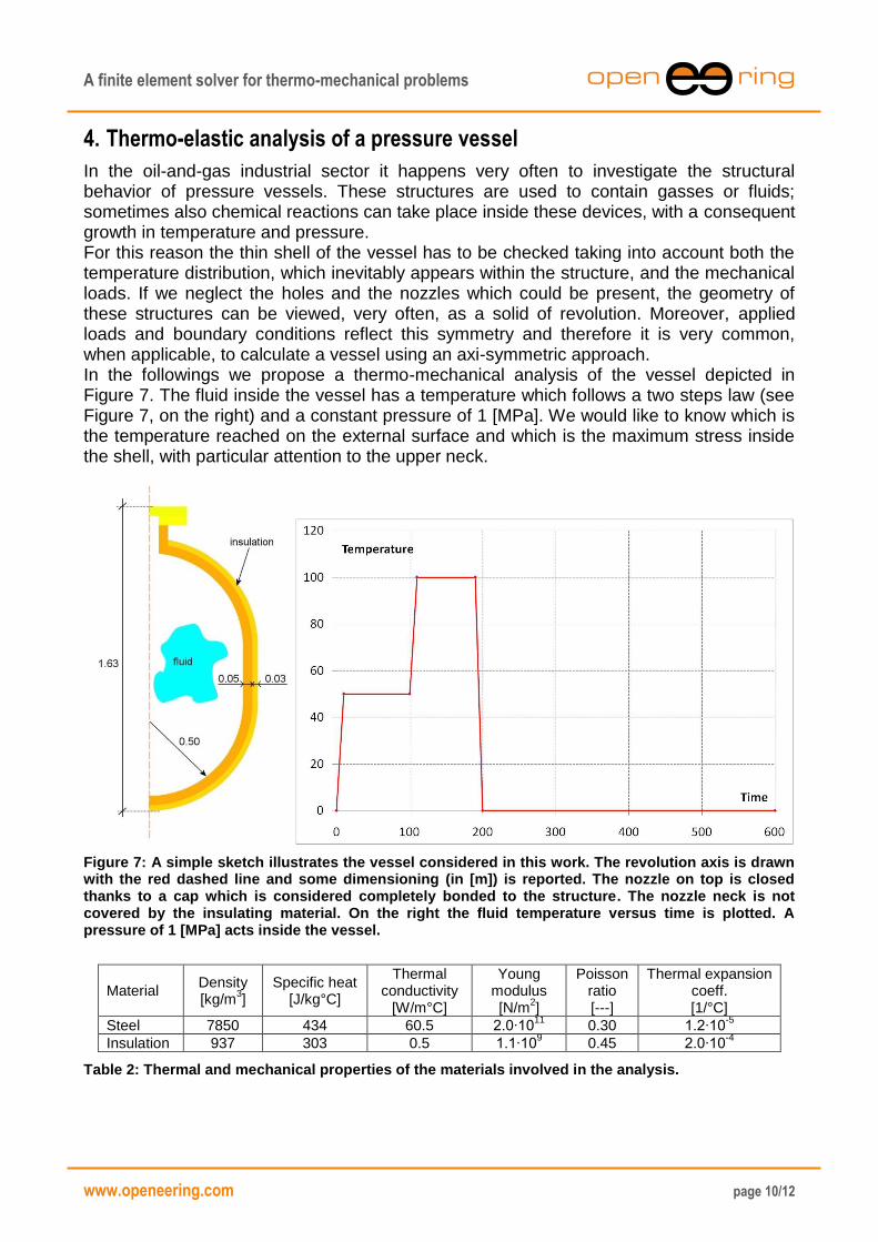
In the oil-and-gas industrial sector it happens very often to investigate the structural behavior of pressure vessels. These structures are used to contain gasses or fluids; sometimes also chemical reactions can take place inside these devices, with a consequent growth in temperature and pressure. For this reason the thin shell of the vessel has to be checked taking into account both the temperature distribution, which inevitably appears within the structure, and the mechanical loads. If we neglect the holes and the nozzles which could be present, the geometry of these structures can be viewed, very often, as a solid of revolution. Moreover, applied loads and boundary conditions reflect this symmetry and therefore it is very common, when applicable, to calculate a vessel using an axi-symmetric approach. In the followings we propose a thermo-mechanical analysis of the vessel depicted in Figure 7. The fluid inside the vessel has a temperature which follows a two steps law (see Figure 7, on the right) and a constant pressure of 1 [MPa]. We would like to know which is the temperature reached on the external surface and which is the maximum stress inside the shell, with particular attention to the upper neck.

Figure 7: A simple sketch illustrates the vessel considered in this work. The revolution axis is drawn with the red dashed line and some dimensioning (in [m]) is reported. The nozzle on top is closed thanks to a cap which is considered completely bonded to the structure. The nozzle neck is not covered by the insulating material. On the right the fluid temperature versus time is plotted. A pressure of 1 [MPa] acts inside the vessel.

Material Density [kg/m

3]

Specific heat [J/kg°C]

Thermal conductivity

[W/m°C]

Young modulus [N/m

2]

Poisson ratio [---]

Thermal expansion coeff. [1/°C]

Steel 7850 434 60.5 2.0∙1011

0.30 1.2∙10-5

Insulation 937 303 0.5 1.1∙109 0.45 2.0∙10

-4

Table 2: Thermal and mechanical properties of the materials involved in the analysis.



We imagine that the vessel is made of common steel and that it has an external thermal insulating cover: the relevant material properties are collected in Table 2. When dealing with a thermo-mechanical problem it could be reasonable to use two different meshes to model and solve the heat transfer and the elasticity equations. Actually, if in the first case we usually are interested in accurate modeling the temperature gradients, in the second case we would like to have a reliable estimation of stress peaks, which in principle could appear in different zones of the domain. For this reason we decided to have the possibility to use different computational grids: once the temperature field is known, it will be mapped on to the structural mesh allowing in this way a better flexibility of our solver. In the case of the pressure vessel we decided to use a uniform mesh within the domain for the thermal solver, while we adopted a finer mesh near the neck for the stress computation. In Figure 8 temperature field at time 150 [s] is drawn: on the right a detail of the neck is plotted. It can be seen that the insulating material plays an important role, the surface temperature is actually maintained very low. As mentioned above a uniform mesh is employed in this case. In Figure 9 the radial (left) and the vertical (right) deformed shapes are plotted. In Figure 10 the von Mises stress is drawn and, on the right, a detail in proximity of the neck is proposed: it can be easily seen that the mesh has been refined in order to better capture the stress peaks in this zone of the vessel.

5. Conclusions

In this work it has been shown how it is possible to use Scilab to solve thermo-mechanical problems. For sake of simplicity the focus has been posed on two dimensional problems but the reader has to remember that the extension to 3D problems does not require any additional effort from a conceptual point of view. Some simple benchmarks have been proposed to show the effectiveness of the solver written in Scilab. The reader should have appreciated the fact that also industrial-like problems can be solved efficiently, as the complete thermo-mechanical analysis of a pressure vessel proposed at the end of the paper.

6. References

[1] http://www.scilab.org/ to have more information on Scilab [2] The Gmsh can be freely downloaded from: http://www.geuz.org/gmsh/ [3] O. C Zienkiewicz, R. L. Taylor, The Finite Element Method: Basic Concepts and Linear Applications (1989) McGraw Hill. [4] M. R. Gosz, Finite Element Method. Applications in Solids, Structures and Heat Transfer (2006) Francis &Taylor. [5] Y. W. Kwon, H. Bang, The Finite Element Method using Matlab, (2006) CRC, 2nd edition

http://www.opensource.org/



Figure 8: The temperature field at time 150 [s] on the left and a detail of the neck on the right, where also the mesh used for the solution of the thermal problem has been superimposed.

Figure 9: Radial (left) and vertical (right) displacement of the vessel.

Figure 10: The von Mises stress and a detail of the neck, on the right, together with the structural mesh.

Documents

A FINITE ELEMENT SOLVER FOR THERMO MECHANICAL · PDF fileA finite element solver for thermo-mechanical problems ... unsteady state heat transfer problem, ... A finite element solver