Embed Size (px)
Citation preview
Journal of Computational and Applied Mathematics 108 (1999) 99–111www.elsevier.nl/locate/cam
A fast algorithm for index of annihilation computationsP.Y. Yalamova;1, M. Mitroulib;∗
aCenter of Applied Mathematics and Informatics, University of Rousse, 7017 Rousse, BulgariabDepartment of Mathematics, University of Athens, Panepistimiopolis 15784, Athens, Greece
Received 8 September 1998; received in revised form 19 February 1999
Abstract
In this paper a fast algorithm for computing the index of annihilation of the associated pencil of a given matrix ispresented. Knowledge of this index leads us to the speci�cation of the elementary divisors of the matrix and thus we canspecify its canonical forms. It is shown that the new algorithm (which is based on the RRQR decomposition) is fasterthan the existing SVD approach. The algorithm can be also applied to matrix pencils and thus specify the structure oftheir elementary divisors. c© 1999 Elsevier Science B.V. All rights reserved.
Keywords: Toeplitz matrix; Paps sequence; Index of annihilation; RRQR decomposition
1. Introduction
The controllability and observability of a linear time-invariant dynamical system of the form
S(A; B; C):{�x′ = A �x + B �u;�y = C �x; (1)
where A∈Rn×n; B∈Rnב; C ∈Rm×n and �x∈Rn, �y∈Rm are real-value vector functions, are in-variant under any equivalence transformation; hence it is conceivable that we may obtain simplercontrollability and observability criteria by transforming the equations of the system into a specialcanonical form. Indeed if a dynamical equation is in a Jordan form, the conditions are very simpleand can be checked almost by inspection. Thus knowledge of the canonical forms of given matricesis the key tool for the study of the basic dynamic and qualitative properties of linear dynamical
∗ Corresponding author.E-mail addresses: [email protected] (P.Y. Yalamov); [email protected] (M. Mitrouli)1 The work of this author was supported by Grants MM-707/97 and I-702/97 from the National Scienti�c Research
Fund of the Bulgarian Ministry of Education and Science.
0377-0427/99/$ - see front matter c© 1999 Elsevier Science B.V. All rights reserved.PII: S 0377-0427(99)00103-X
100 P.Y. Yalamov, M. Mitrouli / Journal of Computational and Applied Mathematics 108 (1999) 99–111
systems of the above form. For any given matrix A∈Rn×n, or Cn×n, the determination of the ele-mentary divisors (ED) of its associated pencil �In−A produces the structure of the similar matricesof A specifying the �rst, second, and Jordan canonical form of A [10, pp. 149–160]. Numericalcomputation of the elementary divisors of a matrix A − �I can be achieved using the staircasealgorithm [3]. It is the aim of the present paper to develop a numerical technique achieving thecomputation of the elementary divisors of a given matrix A∈Rn×n (or Cn×n) using a sparse Toeplitzmatrix approach. Let E be the set containing all the distinct real eigenvalues of this matrix and onlyone member of each complex conjugate pair of eigenvalues.
De�nition 1. Let A∈Rn×n (or Cn×n) be a given matrix. Let �In − A be its associated pencil. Forevery eigenvalue a∈E of matrix A we may de�ne the following sequence of matrices associatedwith �In − A:
P(1)a (In; A) = A− aIn ∈Cn×n; P(2)a (In; A) =[A− aIn 0−In A− aIn
]∈C2n×2n; : : : ;
P(i)a (In; A) =
A− aIn 0 : : : 0 0−In A− aIn : : : 0 0: : : : : : :: : : : : : :: : : : : : :0 0 : : : A− aIn 00 0 : : : −In A− aIn
∈Cin×in: (2)
The rank of the matrix P(i)a (In; A) is denoted by �ia and the corresponding nullity (rank de�ciency)
by nia. The smallest integer �a for which n�aa =n
�a+1a is de�ned as the index of annihilation of �In−A
at �= a.
Let mi be the multiplicity of the ED (�− a)di . The ordered index set:Ia = {(d1; m1); (d2; m2); : : : ; (dp; mp): d1¡d2¡ · · ·¡dp}
characterises the totality of the ED of �In − A at �= a. Let nk=nullity (P(k)a (In − A)); k = 1; 2; : : : ;n0 = 0. Then we have the following results [5].
Lemma 1. The di�erences nk+1 − nk provide the following information about the ED structure of�In − A at �= a.1. n1 − n0 =∑p
j=1mj is the number of ED at �= a.2. The smallest k for which nk+1 − nk = 0 gives the index of annihilation �a; which is also equalto the maximal degree dp.
3. The di�erences nk+1 − nk de�ne the number of ED with degrees higher than k.4. For all k =1; 2; : : : the numbers nk satisfy the relationship nk¿(nk−1 + nk+1)=2. Strict inequalityholds if and only if k is the degree of an ED of �In − A at � = a. Equality holds if and onlyif k is not the degree of an ED.
P.Y. Yalamov, M. Mitrouli / Journal of Computational and Applied Mathematics 108 (1999) 99–111 101
The sequence n0; n1; : : : therefore satis�es arithmetic progression type relationships; the only pointswhere such relationships do not hold are the degrees of the ED. Such a sequence will be referred toas piecewise arithmetic progression sequence (PAPS) of �In−A at �=a. The value of k=d wherethere is a discontinuity in the arithmetic progression relationship will be referred to as a singularpoint and the number �d = 2nd − nd−1 − nd+1 will be called the gap of the sequence at k = d. Thefollowing result [5] relates the PAPS of �In − A at �= a with its index set.
Lemma 2. Let n0; n1; n2; : : : be the PAPS of �In − A at � = a. Then an index k = di is a singularpoint of the sequence; if and only if di is the degree of an ED of �In − A at �= a. If k = di is asingular point; then the gap �di at k = di is equal to the multiplicity mdi of the ED at �= a withthe degree di.
The above approach can be extended to matrix pencils of the form sF − G; F; G ∈Rn×n (orCn×n) by replacing A− aIn with G − aF and −In with −F , where a belongs to the set of roots ofdet(sF−G) [8]. In this way it can be computed the elementary divisors of the pencils and thereforederive canonical forms for them.In [5] it has been developed a numerical algorithm concerning the evaluation of the elementary
divisors of a matrix through the PAPS approach. The most important numerical problems arisingare:(P1) Numerical determination of the set E.By applying an appropriate numerical technique based on the Schur Decomposition
[6, pp. 361–382] we compute a triangular matrix T containing the eigenvalues in its diagonalblocks. In the sequel, when the given matrix is a small perturbation of a matrix with true mul-tiple eigenvalues we select the corresponding numerical multiple eigenvalues by sorting the diag-onal elements of the triangular matrix T , so that possible numerical multiple eigenvalues (closeeigenvalues) appear in adjacent positions. Then use the Gerschgorin circles constructed for diag-onal similarity transformations of the matrix to decide which of the eigenvalue approximationsform groups corresponding to numerical multiple eigenvalues. The grouping strategy is describedin [11]. When a group is found whose eigenvalues are isolated from the rest of the eigenval-ues, but not from each other, the mean of the diagonal elements is taken as a numerical multipleeigenvalue.(P2) Appropriate numerical implementation of the PAPS sequence.In the PAPS approach each matrix P(k)a (In; A) = A
(k) has a speci�c structure. It is a quite sparseblock Toeplitz matrix. This special structure is not utilized in [5] where the computations of theindex of annihilation are performed directly by using the singular value decomposition (SVD) of A(k)
and, thus, the SVD is computed from the beginning for each matrix A(k). In this case the time andthe memory needed for each updating step become very large when k grows. One way to proposea faster algorithm is to use updating of some rank revealing decomposition (see [1,2]). Therefore,in this paper we develop another algorithm which fully exploits the structure of the matrices A(k):This algorithm is very fast because it needs rank-revealing factorizations of matrices having sizeonly [n+O(1)]× [n+O(1)]. The memory needed is for a few matrices of the same size, i.e. O(n2)for a dense matrix A.The outline of the paper is as follows. In Section 2 we review brie y the rank revealing QR
decomposition (RRQR). Then in Section 3 the new algorithm for index of annihilation computations
102 P.Y. Yalamov, M. Mitrouli / Journal of Computational and Applied Mathematics 108 (1999) 99–111
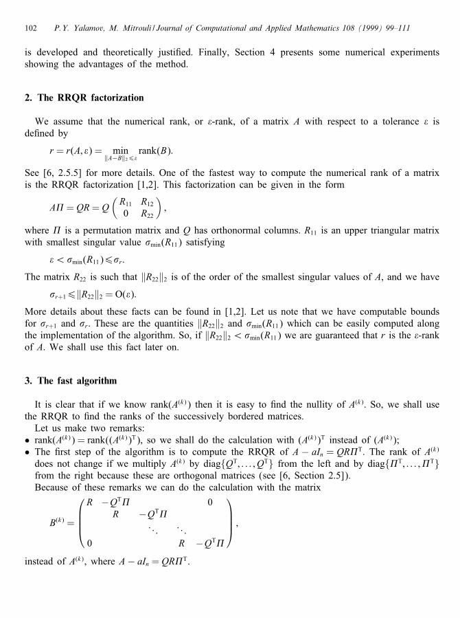
is developed and theoretically justi�ed. Finally, Section 4 presents some numerical experimentsshowing the advantages of the method.
2. The RRQR factorization
We assume that the numerical rank, or �-rank, of a matrix A with respect to a tolerance � isde�ned by
r = r(A; �) = min‖A−B‖26�
rank(B):
See [6, 2.5.5] for more details. One of the fastest way to compute the numerical rank of a matrixis the RRQR factorization [1,2]. This factorization can be given in the form
A� = QR= Q(R11 R120 R22
);
where � is a permutation matrix and Q has orthonormal columns. R11 is an upper triangular matrixwith smallest singular value �min(R11) satisfying
�¡�min(R11)6�r:
The matrix R22 is such that ‖R22‖2 is of the order of the smallest singular values of A, and we have�r+16‖R22‖2 = O(�):
More details about these facts can be found in [1,2]. Let us note that we have computable boundsfor �r+1 and �r: These are the quantities ‖R22‖2 and �min(R11) which can be easily computed alongthe implementation of the algorithm. So, if ‖R22‖2¡�min(R11) we are guaranteed that r is the �-rankof A: We shall use this fact later on.
3. The fast algorithm
It is clear that if we know rank(A(k)) then it is easy to �nd the nullity of A(k): So, we shall usethe RRQR to �nd the ranks of the successively bordered matrices.Let us make two remarks:
• rank(A(k)) = rank((A(k))T), so we shall do the calculation with (A(k))T instead of (A(k));• The �rst step of the algorithm is to compute the RRQR of A − aIn = QR�T: The rank of A(k)
does not change if we multiply A(k) by diag{QT; : : : ; QT} from the left and by diag{�T; : : : ; �T}from the right because these are orthogonal matrices (see [6, Section 2.5]).Because of these remarks we can do the calculation with the matrix
B(k) =
R −QT� 0
R −QT�. . . . . .
0 R −QT�
;
instead of A(k), where A− aIn = QR�T.
P.Y. Yalamov, M. Mitrouli / Journal of Computational and Applied Mathematics 108 (1999) 99–111 103
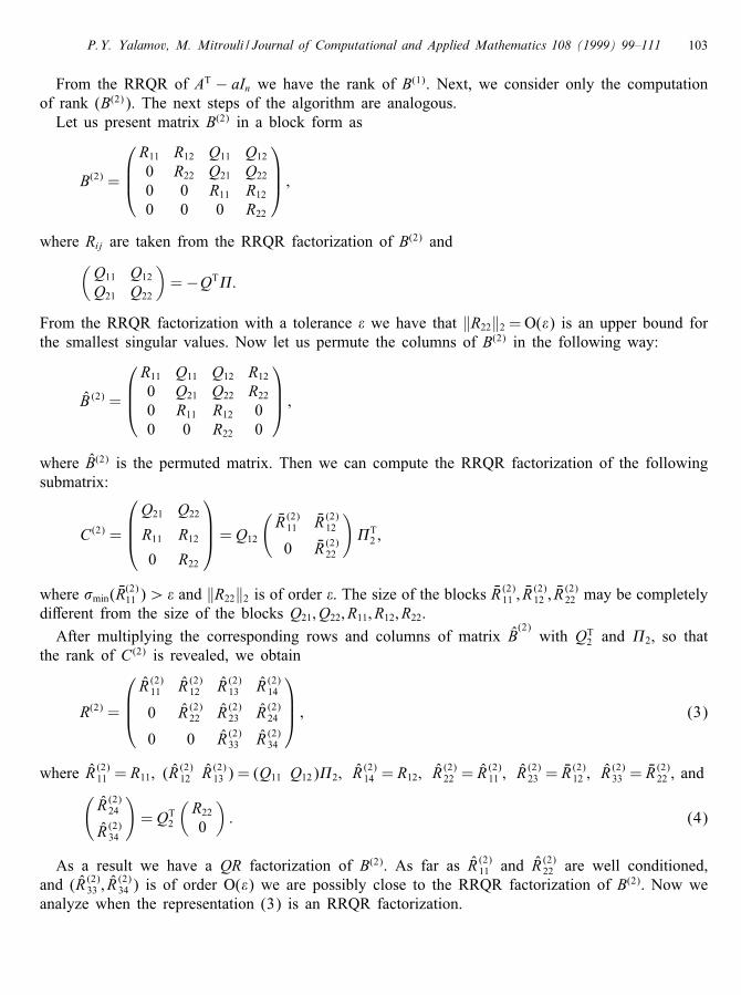
From the RRQR of AT − aIn we have the rank of B(1). Next, we consider only the computationof rank (B(2)). The next steps of the algorithm are analogous.Let us present matrix B(2) in a block form as
B(2) =
R11 R12 Q11 Q120 R22 Q21 Q220 0 R11 R120 0 0 R22
;
where Rij are taken from the RRQR factorization of B(2) and(Q11 Q12Q21 Q22
)=−QT�:
From the RRQR factorization with a tolerance � we have that ‖R22‖2 = O(�) is an upper bound forthe smallest singular values. Now let us permute the columns of B(2) in the following way:
B̂ (2) =
R11 Q11 Q12 R120 Q21 Q22 R220 R11 R12 00 0 R22 0
;
where B̂(2) is the permuted matrix. Then we can compute the RRQR factorization of the followingsubmatrix:
C(2) =
Q21 Q22R11 R120 R22
= Q12
(�R (2)11 �R (2)120 �R (2)22
)�T2 ;
where �min( �R(2)11 )¿� and ‖R22‖2 is of order �. The size of the blocks �R (2)11 ; �R (2)12 ; �R (2)22 may be completely
di�erent from the size of the blocks Q21; Q22; R11; R12; R22:After multiplying the corresponding rows and columns of matrix B̂
(2)with QT2 and �2; so that
the rank of C(2) is revealed, we obtain
R(2) =
R̂ (2)11 R̂ (2)12 R̂ (2)13 R̂ (2)140 R̂ (2)22 R̂ (2)23 R̂ (2)240 0 R̂ (2)33 R̂ (2)34
; (3)
where R̂ (2)11 = R11; (R̂(2)12 R̂
(2)13 ) = (Q11 Q12)�2; R̂
(2)14 = R12; R̂
(2)22 = R̂
(2)11 ; R̂
(2)23 = �R (2)12 ; R̂
(2)33 = �R (2)22 ; and(
R̂ (2)24R̂ (2)34
)= QT2
(R220
): (4)
As a result we have a QR factorization of B(2): As far as R̂ (2)11 and R̂(2)22 are well conditioned,
and (R̂ (2)33 ; R̂(2)34 ) is of order O(�) we are possibly close to the RRQR factorization of B
(2): Now weanalyze when the representation (3) is an RRQR factorization.
104 P.Y. Yalamov, M. Mitrouli / Journal of Computational and Applied Mathematics 108 (1999) 99–111
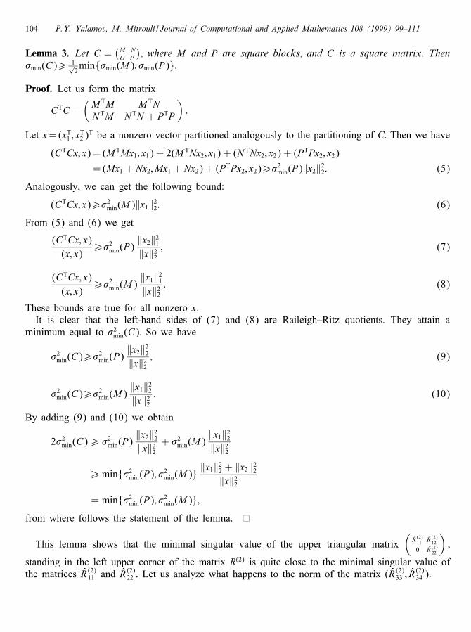
Lemma 3. Let C =(M NO P
); where M and P are square blocks; and C is a square matrix. Then
�min(C)¿ 1√2min{�min(M); �min(P)}.
Proof. Let us form the matrix
CTC =(M TM M TNN TM N TN + PTP
):
Let x=(xT1 ; xT2 )T be a nonzero vector partitioned analogously to the partitioning of C: Then we have
(CTCx; x) = (M TMx1; x1) + 2(M TNx2; x1) + (N TNx2; x2) + (PTPx2; x2)
= (Mx1 + Nx2; Mx1 + Nx2) + (PTPx2; x2)¿�2min(P)‖x2‖22: (5)
Analogously, we can get the following bound:
(CTCx; x)¿�2min(M)‖x1‖22: (6)
From (5) and (6) we get
(CTCx; x)(x; x)
¿�2min(P)‖x2‖21‖x‖22
; (7)
(CTCx; x)(x; x)
¿�2min(M)‖x1‖21‖x‖22
: (8)
These bounds are true for all nonzero x.It is clear that the left-hand sides of (7) and (8) are Raileigh–Ritz quotients. They attain a
minimum equal to �2min(C): So we have
�2min(C)¿�2min(P)
‖x2‖22‖x‖22
; (9)
�2min(C)¿�2min(M)
‖x1‖22‖x‖22
: (10)
By adding (9) and (10) we obtain
2�2min(C)¿ �2min(P)‖x2‖22‖x‖22
+ �2min(M)‖x1‖22‖x‖22
¿min{�2min(P); �2min(M)}‖x1‖22 + ‖x2‖22
‖x‖22= min{�2min(P); �2min(M)};
from where follows the statement of the lemma.
This lemma shows that the minimal singular value of the upper triangular matrix(R̂ (2)11 R̂ (2)120 R̂ (2)22
);
standing in the left upper corner of the matrix R(2) is quite close to the minimal singular value ofthe matrices R̂ (2)11 and R̂
(2)22 . Let us analyze what happens to the norm of the matrix (R̂ (2)33 ; R̂
(2)34 ):
P.Y. Yalamov, M. Mitrouli / Journal of Computational and Applied Mathematics 108 (1999) 99–111 105
Lemma 4. The norm of the matrix (R̂ (2)33 ; R̂(2)34 ) is bounded as follows:
‖(R̂ (2)33 ; R̂ (2)34 )‖26√‖R̂ (2)33 ‖22 + ‖R22‖22:
Proof. For any matrix of the form C = (M N ) it is easy to see that
(CCTx; x)(x; x)
=(MM Tx; x)(x; x)
+(NN Tx; x)(x; x)
6 ‖M‖22 + ‖N‖22;from where it follows that:
‖C‖226‖M‖22 + ‖N‖22:So, we have
‖(R̂ (2)33 ; R̂ (2)34 )‖26√‖R̂ (2)33 ‖22 + ‖R̂ (2)34 ‖2:
But from (4) we get
‖R̂ (2)34 ‖6‖R22‖2;and thus we have the statement of the lemma.
Lemma 2 shows that if ‖R22‖2 and ‖R(2)33 ‖2 are small, then the matrix in the right lower corner ofR(2) is also of small norm. Let us note that R22 and R
(2)33 have small norms (of order O(�)) because
they come from the RRQR factorization of some matrices.From the two lemmas we have the following obvious theorem:
Theorem 1. If
min{�min(R(2)11 ); �min(R(2)22 )}¿ ‖(R(2)33 ; R(1)34 )‖2; (11)
then R(2) is the R-factor of the RRQR factorization of B(2):
So, we can write
R(2) =
(R(2)11 R(2)120 R(2)22
);
where
R(2)11 =
(R̂ (2)11 R̂ (2)120 R̂ (2)22
); R(2)12 =
(R̂ (2)13 R̂ (2)14R̂ (2)23 R̂ (2)24
);
R(2)22 = (R̂(2)33 ; R̂
(2)34 );
and we have from Lemma 1 a lower bound for �min(R(2)11 ); and from Lemma 2 an upper bound for
‖R(2)22 ‖2:
106 P.Y. Yalamov, M. Mitrouli / Journal of Computational and Applied Mathematics 108 (1999) 99–111
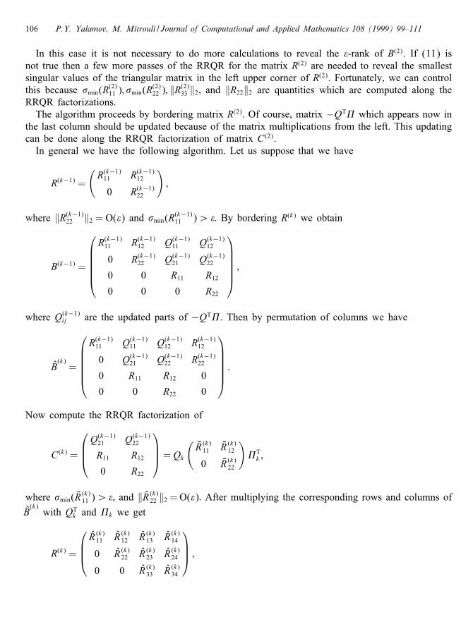
In this case it is not necessary to do more calculations to reveal the �-rank of B(2). If (11) isnot true then a few more passes of the RRQR for the matrix R(2) are needed to reveal the smallestsingular values of the triangular matrix in the left upper corner of R(2). Fortunately, we can controlthis because �min(R
(2)11 ); �min(R
(2)22 ); ‖R(2)33 ‖2; and ‖R22‖2 are quantities which are computed along the
RRQR factorizations.The algorithm proceeds by bordering matrix R(2): Of course, matrix −QT� which appears now in
the last column should be updated because of the matrix multiplications from the left. This updatingcan be done along the RRQR factorization of matrix C(2).In general we have the following algorithm. Let us suppose that we have
R(k−1) =
(R(k−1)11 R(k−1)12
0 R(k−1)22
);
where ‖R(k−1)22 ‖2 = O(�) and �min(R(k−1)11 )¿�: By bordering R(k) we obtain
B(k−1) =
R(k−1)11 R(k−1)12 Q(k−1)11 Q(k−1)12
0 R(k−1)22 Q(k−1)21 Q(k−1)22
0 0 R11 R120 0 0 R22
;
where Q(k−1)ij are the updated parts of −QT�. Then by permutation of columns we have
B̂(k)=
R(k−1)11 Q(k−1)11 Q(k−1)12 R(k−1)12
0 Q(k−1)21 Q(k−1)22 R(k−1)22
0 R11 R12 0
0 0 R22 0
:
Now compute the RRQR factorization of
C(k) =
Q(k−1)21 Q(k−1)22
R11 R120 R22
= Qk
(�R (k)11 �R (k)120 �R (k)22
)�Tk ;
where �min( �R(k)11 )¿�; and ‖ �R (k)22 ‖2 =O(�): After multiplying the corresponding rows and columns of
B̂(k)with QTk and �k we get
R(k) =
R̂ (k)11 R̂ (k)12 R̂ (k)13 R̂ (k)140 R̂ (k)22 R̂ (k)23 R̂ (k)240 0 R̂ (k)33 R̂ (k)34
;
P.Y. Yalamov, M. Mitrouli / Journal of Computational and Applied Mathematics 108 (1999) 99–111 107
where R̂ (k)11 = R̂(k−1)12 ; (R̂ (k)12 ; R̂
(k)13 ) = (Q̂
(k−1)11 ; Q̂(k−1)12 )�k; R̂
(k)14 = R̂
(k−1)12 ; R̂ (k)22 = �R (k)11 ; R̂
(k)23 = �R (k)12 ; R̂
(k)33 =
�R (k−1)22 ; and(R̂ (k)24R̂ (k)34
)= QTk
(R(k−1)22
0
):
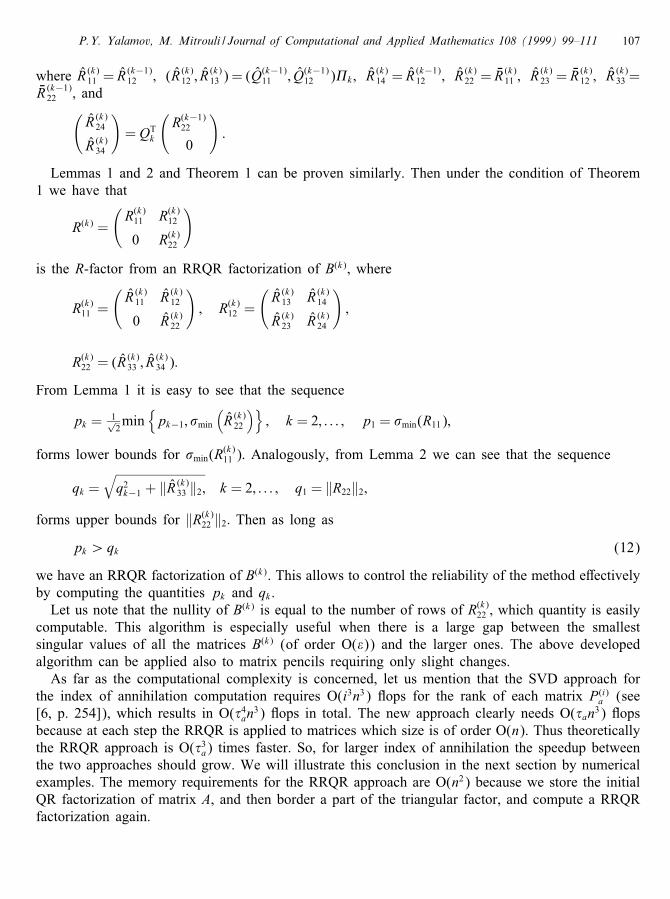
Lemmas 1 and 2 and Theorem 1 can be proven similarly. Then under the condition of Theorem1 we have that
R(k) =
(R(k)11 R(k)120 R(k)22
)
is the R-factor from an RRQR factorization of B(k); where
R(k)11 =
(R̂ (k)11 R̂ (k)120 R̂ (k)22
); R(k)12 =
(R̂ (k)13 R̂ (k)14R̂ (k)23 R̂ (k)24
);
R(k)22 = (R̂(k)33 ; R̂
(k)34 ):
From Lemma 1 it is easy to see that the sequence
pk = 1√2min
{pk−1; �min
(R̂ (k)22
)}; k = 2; : : : ; p1 = �min(R11);
forms lower bounds for �min(R(k)11 ): Analogously, from Lemma 2 we can see that the sequence
qk =√q2k−1 + ‖R̂ (k)33 ‖2; k = 2; : : : ; q1 = ‖R22‖2;
forms upper bounds for ‖R(k)22 ‖2: Then as long aspk ¿qk (12)
we have an RRQR factorization of B(k). This allows to control the reliability of the method e�ectivelyby computing the quantities pk and qk .Let us note that the nullity of B(k) is equal to the number of rows of R(k)22 ; which quantity is easily
computable. This algorithm is especially useful when there is a large gap between the smallestsingular values of all the matrices B(k) (of order O(�)) and the larger ones. The above developedalgorithm can be applied also to matrix pencils requiring only slight changes.As far as the computational complexity is concerned, let us mention that the SVD approach for
the index of annihilation computation requires O(i3n3) ops for the rank of each matrix P(i)a (see[6, p. 254]), which results in O(�4an
3) ops in total. The new approach clearly needs O(�an3) opsbecause at each step the RRQR is applied to matrices which size is of order O(n). Thus theoreticallythe RRQR approach is O(�3a) times faster. So, for larger index of annihilation the speedup betweenthe two approaches should grow. We will illustrate this conclusion in the next section by numericalexamples. The memory requirements for the RRQR approach are O(n2) because we store the initialQR factorization of matrix A, and then border a part of the triangular factor, and compute a RRQRfactorization again.
108 P.Y. Yalamov, M. Mitrouli / Journal of Computational and Applied Mathematics 108 (1999) 99–111
Concerning the numerical stability of the proposed algorithm we have to note that if U is ortho-gonal, and M (1) = UM ∈Rn×n then
U (M +�M) = M̃(1); ‖�M‖26(2n− 3)‖M‖2 �0 + O(�20);
where �M is the equivalent perturbation of matrix M (see [12]), and �0 is the machine precision.The last result can be found in [4], for example. As far as we apply several orthogonal transforma-tions to matrix P(�a)a it is clear that for the whole algorithm we have
U (P(�a)a +�P(�a)a ) = P̃; ‖�P(�a)a ‖26cn‖P(�a)a ‖2�0;where U is orthogonal (a product of orthogonal matrices), and cn is a constant linearly depending onn. Thus the RRQR approach is backward stable. Let us note that perturbations in inputs of similarsize as those of �M will not change the output of the algorithm essentially. So, this algorithm isnot sensitive to input perturbations of order cn‖P(�a)a ‖2�0.
4. Numerical results
The new algorithm is tested in MATLAB with a machine roundo� unit 2:22× 10−16. For thepresentation of the examples three signi�cant digits will be kept. We count the number of opsby the corresponding function of MATLAB. The rank computations are controlled by the toleranceparameter � which is an input for the RRQR procedure.We choose the examples below so that di�erent practical situations are simulated. Example 1 is a
well-conditioned problem, Example 2 is ill-conditioned, Example 3 illustrates the case when manybordering steps are needed, and Example 4 is an application of the method to matrix pencils.
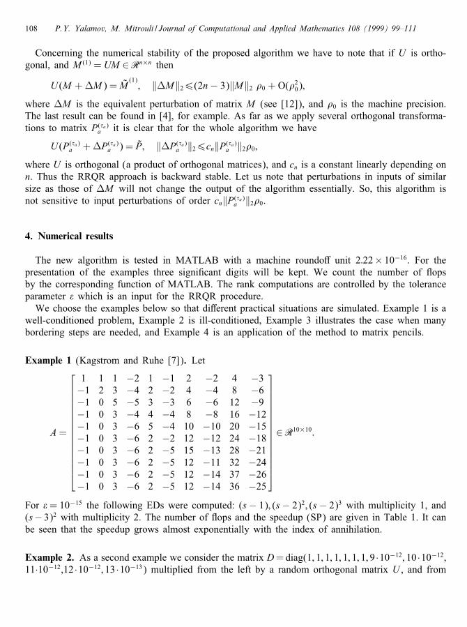
Example 1 (Kagstrom and Ruhe [7]). Let
A=
1 1 1 −2 1 −1 2 −2 4 −3−1 2 3 −4 2 −2 4 −4 8 −6−1 0 5 −5 3 −3 6 −6 12 −9−1 0 3 −4 4 −4 8 −8 16 −12−1 0 3 −6 5 −4 10 −10 20 −15−1 0 3 −6 2 −2 12 −12 24 −18−1 0 3 −6 2 −5 15 −13 28 −21−1 0 3 −6 2 −5 12 −11 32 −24−1 0 3 −6 2 −5 12 −14 37 −26−1 0 3 −6 2 −5 12 −14 36 −25
∈R10×10:
For �= 10−15 the following EDs were computed: (s− 1); (s− 2)2; (s− 2)3 with multiplicity 1, and(s− 3)2 with multiplicity 2. The number of ops and the speedup (SP) are given in Table 1. It canbe seen that the speedup grows almost exponentially with the index of annihilation.
Example 2. As a second example we consider the matrix D=diag(1; 1; 1; 1; 1; 1; 1; 9 ·10−12; 10 ·10−12;11·10−12,12 ·10−12; 13 ·10−13) multiplied from the left by a random orthogonal matrix U , and from
P.Y. Yalamov, M. Mitrouli / Journal of Computational and Applied Mathematics 108 (1999) 99–111 109
Table 1The number of ops for the SVD and the RRQR approach and the speedup SP for Example 1
a 1 2 3
SVD 35 997 324 409 123 495RRQR 14 528 36 634 26 186SP 2.48 8.86 4.72
Table 2The number of ops for the SVD and the RRQR approach and the speedup SP for Example 2
a 1 � = 10−13 � = 10−11
SVD 55 263 — 56 199RRQR 38 812 23 296 31 410SP 1.42 — 1.79
the right by U T. Thus, this matrix has some small eigenvalues which can be considered equal depend-ing on the tolerance used. First, we compute the index of annihilation for all the eigenvalues with atolerance �=10−13. In this case the algorithm produces one ED (s−1) with multiplicity 7, and �vedi�erent EDs with multiplicities 1 (the SVD approach cannot discriminate this case). Then we dothe same computation but with a tolerance �=10−11 (a number larger than the smaller eigenvalues).As should be expected the di�erence now is that the algorithm produces one ED with multiplicity5 (corresponding to the smallest eigenvalues). The number of ops and the speedup are given inTable 2, where the last two columns give the results for any small eigenvalue with di�erent toler-ances. Let us also note that in this example we added small perturbations of order 10−14 to eachentry of the original matrix. All the results are the same in the case of perturbations. This showsthat the new algorithm behaves in a stable way.
Example 3. In this example we would like to see how the algorithms behaves when we have arelatively large number of bordering steps. For this purpose we need eigenvalues with large Jordancells. First we generated a Jordan matrix with two Jordan cells each of size n:
J1 =
1 11 1. . . . . .
1 11
; J2 =
2 12 1. . . . . .
2 12
:
Then we produced the matrix A = P−1JP, where P = tridiag(a; b; a); a = (−1; : : : ;−1); b =(1; 2; : : : ; 2). We chose this type of matrix P because its inverse is known explicitly, the entriesof matrix A are integers, and there is no roundo� errors involved when forming matrix A. In thisway we know exactly its eigenvalues, and can watch the accuracy of our algorithm. The toleranceis chosen by default in the RRQR factorization. For the choice of n = 20; 40; : : : ; 80 the algorithm
110 P.Y. Yalamov, M. Mitrouli / Journal of Computational and Applied Mathematics 108 (1999) 99–111
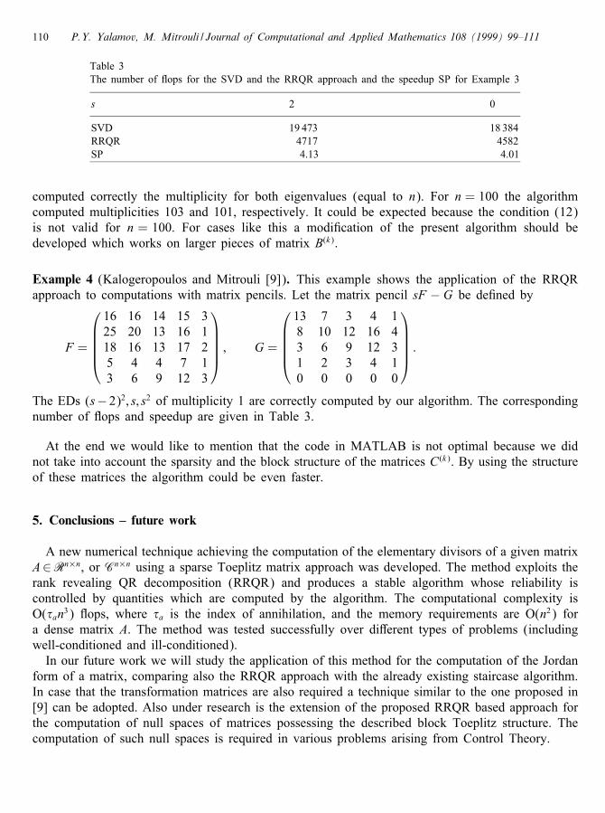
Table 3The number of ops for the SVD and the RRQR approach and the speedup SP for Example 3
s 2 0
SVD 19 473 18 384RRQR 4717 4582SP 4.13 4.01
computed correctly the multiplicity for both eigenvalues (equal to n). For n = 100 the algorithmcomputed multiplicities 103 and 101, respectively. It could be expected because the condition (12)is not valid for n = 100. For cases like this a modi�cation of the present algorithm should bedeveloped which works on larger pieces of matrix B(k).
Example 4 (Kalogeropoulos and Mitrouli [9]). This example shows the application of the RRQRapproach to computations with matrix pencils. Let the matrix pencil sF − G be de�ned by
F =
16 16 14 15 325 20 13 16 118 16 13 17 25 4 4 7 13 6 9 12 3
; G =
13 7 3 4 18 10 12 16 43 6 9 12 31 2 3 4 10 0 0 0 0
:
The EDs (s−2)2; s; s2 of multiplicity 1 are correctly computed by our algorithm. The correspondingnumber of ops and speedup are given in Table 3.
At the end we would like to mention that the code in MATLAB is not optimal because we didnot take into account the sparsity and the block structure of the matrices C(k). By using the structureof these matrices the algorithm could be even faster.
5. Conclusions – future work
A new numerical technique achieving the computation of the elementary divisors of a given matrixA∈Rn×n, or Cn×n using a sparse Toeplitz matrix approach was developed. The method exploits therank revealing QR decomposition (RRQR) and produces a stable algorithm whose reliability iscontrolled by quantities which are computed by the algorithm. The computational complexity isO(�an3) ops, where �a is the index of annihilation, and the memory requirements are O(n2) fora dense matrix A. The method was tested successfully over di�erent types of problems (includingwell-conditioned and ill-conditioned).In our future work we will study the application of this method for the computation of the Jordan
form of a matrix, comparing also the RRQR approach with the already existing staircase algorithm.In case that the transformation matrices are also required a technique similar to the one proposed in[9] can be adopted. Also under research is the extension of the proposed RRQR based approach forthe computation of null spaces of matrices possessing the described block Toeplitz structure. Thecomputation of such null spaces is required in various problems arising from Control Theory.
P.Y. Yalamov, M. Mitrouli / Journal of Computational and Applied Mathematics 108 (1999) 99–111 111
Acknowledgements
The authors are thankful to Per Christian Hansen who was so kind to allow the usage of theRRQR MATLAB implementation for the numerical tests. We also thank the anonymous refereesfor their suggestions to improve the numerical examples.
Reference
[1] T.F. Chan, P.C. Hansen, Some applications of the rank revealing QR factorization, SIAM J. Sci. Statist. Comput.13 (1992) 727–741.
[2] T.F. Chan, Rank revealing QR factorizations, Linear Algebra Appl. 88/89 (1987) 67–82.[3] J. Demmel, A. Edelman, The dimension of matrices (matrix pencils) with given Jordan (Kronecker) canonical forms,
Linear Algebra Appl. 230 (1995) 61–87.[4] M. Gentleman, Error Analysis of QR decomposition by Givens transformations, Linear Algebra Appl. 10 (1973)
189–197.[5] M. Mitrouli, G. Kalogeropoulos, A matrix pencil approach computing the elementary divisors of a matrix: Numerical
aspects and applications, Korean J. Computat. Appl. Math. 5 (3) (1998) 627–644.[6] G.H. Golub, C.F. van Loan, Matrix Computations, 3rd Edition, John Hopkins University Press, Baltimore, MD,
1996.[7] B. Kagstrom, A. Ruhe, An algorithm for numerical computation of the Jordan normal form of a complex matrix,
ACM Trans. Math. Software 6 (3) (1980) 398–419.[8] G. Kalogeropoulos, M. Mitrouli, On the computation of the Weierstrass canonical form of a regular matrix pencil,
Control Comput. 19 (3) (1991) 71–75.[9] G. Kalogeropoulos, M. Mitrouli, On the computation of the Weierstrass canonical form of a regular matrix pencil:
Part II, Control Comput. 22 (1) (1994) 18–22.[10] P. Lancaster, Theory of Matrices, Academic Press, New York, 1969.[11] A. Ruhe, An algorithm for numerical determination of the structure of a general matrix, BIT 10 (1970) 196–216.[12] J. Wilkinson, The Algebraic Eigenvalue Problem, Oxford University Press, Oxford, 1988.


![RNS Modular Computations for Cryptographic Applications...Algo. EMM EMW Our algorithm 5n2 + 17n 3n2 + 20n RNS-ME [GLP+12] 6n2 + 12n 2n2 + 10n Our algorithm (regular) 6n ...Author:](https://img.dokumen.tips/doc/110x75/6141bb47d64cc55ff0755b97/rns-modular-computations-for-cryptographic-applications-algo-emm-emw-our-algorithm.jpg)