A dynamic reformulation heuristicfor Generalized Interdiction Problems

Matteo Fischetti

Department of Information Engineering, University of Padua, Italy

Michele Monaci

DEI, University of Bologna, Italy

Markus Sinnl

Department of Statistics and Operations Research, University of Vienna, Austria

Abstract

We consider a subfamily of mixed-integer linear bilevel problems that we call Generalized Interdiction

Problems. This class of problems includes, among others, the widely-studied interdiction problems, i.e.,

zero-sum Stackelberg games where two players (called the leader and the follower) share a set of items, and

the leader can interdict the usage of certain items by the follower. Problems of this type can be modeled

as Mixed-Integer Nonlinear Programming problems, whose exact solution can be very hard. In this paper

we propose a new heuristic scheme based on a single-level and compact mixed-integer linear programming

reformulation of the problem obtained by relaxing the integrality of the follower variables. A distinguished

feature of our method is that general-purpose mixed-integer cutting planes for the follower problem are

exploited, on the fly, to dynamically improve the reformulation. The resulting heuristic algorithm proved

very effective on a large number of test instances, often providing an (almost) optimal solution within very

short computing times.

Keywords: (O) Combinatorial optimization; bilevel optimization; interdiction problems; mixed-integer

programming; heuristics.

IA dynamic reformulation heuristic for generalized interdiction problemsEmail addresses: matteo.fischetti@unipd.it (Matteo Fischetti), michele.monaci@unibo.it (Michele Monaci),

markus.sinnl@univie.ac.at (Markus Sinnl)

Preprint submitted to Elsevier August 5, 2017

1. Introduction

A general bilevel optimization problem is defined as

minx∈Rn1

F (x, y) (1)

G(x, y) ≤ 0 (2)

y ∈ arg maxy′∈Rn2

{f(x, y′) : g(x, y′) ≤ 0 }, (3)

where F, f : Rn1+n2 → R, G : Rn1+n2 → Rm1 , and g : Rn1+n2 → Rm2 . Let n = n1 + n2 denote the total

number of decision variables.

We will refer to x and y as the leader and follower decision variable vectors, respectively. Accordingly,

F (x, y) and G(x, y) ≤ 0 denote the leader objective function and constraints, while (3) defines the follower

subproblem. In case the follower subproblem has multiple optimal solutions, we assume that one with

minimum leader cost among those with G(x, y) ≤ 0 is chosen, i.e., we consider the optimistic version of

bilevel optimization [1].

By defining the follower value function for a given leader vector x ∈ Rn1 as

Φ(x) = maxy′∈Rn2

{f(x, y′) : g(x, y′) ≤ 0 }, (4)

one can restate the bilevel optimization problem through the so-called value-function reformulation [2] below:

minx,y

F (x, y) (5)

G(x, y) ≤ 0 (6)

g(x, y) ≤ 0 (7)

(x, y) ∈ Rn (8)

f(x, y) ≥ Φ(x). (9)

Problem (5)-(8) is usually called the High-Point Relaxation (HPR), which is used in many solution approaches

to bilevel programming, including [3, 4].

A Mixed-Integer Bilevel Linear Problem (MIBLP) is a bilevel problem in which both objective functions

F (x, y) and f(x, y) are linear (or affine), and each constraint in G(x, y) ≤ 0 and in g(x, y) ≤ 0 is either a

linear inequality, or stipulates the integrality of a certain component of (x, y).

Relevant special cases of MIBLPs are known as interdiction problems (or interdiction games). They can

be seen as a special class of zero-sum Stackelberg games [5], i.e., models in which a leader takes some decision

and a follower reacts in a sequential way. While in general Stackelberg games the objective functions of the

leader and of the follower are different from each other, in interdiction problems the two problems optimize

over the same objective function, but in the opposite direction. In addition, in these problems the leader

2

takes decisions that fix some follower variables to zero [6]. Thus, the leader and the follower share a set of

items, and the connection between the leader and the follower optimization problems is established through

binary “interdiction variables” that are controlled by the leader—a leader solution x being sometimes called

interdiction policy in this context. Interdiction problems model important applications including marketing

[3], defense of critical infrastructures [7, 8], and fighting of drug smuggling [9] and illegal nuclear projects

[10, 11].

Contribution. Our main contributions can be summarized as follows.

• We introduce a generalization of the interdiction problems typically addressed in the literature. This

variant of problems, to be formally described in Section 3, is obtained by removing the assumption

that the leader and follower linear objective functions are one the opposite of the other. Generalized

interdiction problems cannot be cast as min-max or max-min problems, so many classical results that

hold for standard interdiction problems need to be generalized to the new setting.

• For such generalized interdiction problems, we consider the relaxation obtained by dropping the inte-

grality requirement in the follower, obtaining a bilevel problem that can be reformulated into a standard

(i.e., single-level and compact) Mixed-Integer Linear Program (MILP). Similar reformulations have

been addressed in the literature for standard interdiction problems both with a MILP follower (e.g., in

[12, 13, 14]) and with an LP follower (in this latter case, the reformulation is equivalent to the original

problem; see, e.g., [15, 16, 17]). Moreover, for another class of min-max problems, namely the min-max

regret robust problems, a related relax-dualise-reformulate idea has been used to devise heuristics (e.g.,

in [18, 19]). As far as we know, however, the min-max reformulations from the literature were never

extended to the generalized interdiction setting we consider in the present paper.

• We describe two basic interdiction heuristics based on the solution of the reformulated problem through

a black-box MILP solver, and on the application of refinement procedures to derive a bilevel feasible

solution. While these two heuristics are in the spirit of [12, 14], we propose an improved version

based on a dynamic reformulation. This latter algorithm iteratively generates, on the fly, valid cutting

planes based on the integrality of the follower variables, thus producing improved reformulations and

better solutions. The resulting approach can be viewed as a (row and) column generation method

applied to the reformulation, whose effectiveness has been confirmed by extensive computational tests.

To the best of our knowledge, a similar mechanism was never used in the context of general-purpose

interdiction or min-max heuristics.

• Our heuristic solution scheme can easily be adapted to more general min-max problems, and also to

the setting addressed in [15] where interdiction penalties (as opposed to constraints) are considered.

3

• We report very extensive computational tests on more than 1200 instances both from the literature

and randomly generated. This is, by far, the most extensive study on general-purpose interdiction

heuristics reported in the literature. The outcome of our experiments is that, although quite simple,

even the most basic variant of our heuristic is quite successful for a large number of instances, often

providing an optimal solution within negligible computing time. For the hardest instances, however,

our more sophisticated version based on the dynamic reformulation gives a significant performance

improvement.

The paper is organized as follows. Previous work on interdiction problems and heuristic methods for

bilevel (integer) linear programming problems is briefly surveyed in Section 2. The generalized interdiction

problem we address in our work is mathematically stated in Section 3, while a single-level compact reformu-

lation of the problem without integrality requirement on the y variables is introduced in Section 4. Section 5

describes our basic heuristic along with two extensions intended to produce improved solutions. Extensive

computational results on various classes of test instances are reported in Section 6, while Section 7 draws

some conclusions and addresses future directions of work.

2. Previous work

We next focus on previous work regarding interdiction problems. For the sake of completeness, we also

briefly outline heuristic approaches for bilevel (integer) linear programming, and refer the reader to, e.g., [4],

for previous work on exact approaches for MIBLP.

Exact Solvers for Interdiction Problems. When the follower problem in an interdiction problem can be

formulated as linear program, duality-based reformulations give exact algorithms. This idea has been used,

e.g., in [17] for the maximum flow problem, in [16] for multi-commodity flow problems, and in [20] for the

spanning tree problems. The shortest-path variant for a problem where interdiction does not forbid the

use of an item but causes a penalty in the follower objective is studied in [15], where a duality-based exact

algorithm is given. Finally, for another variant where interdiction is not a discrete decision, but continuously

increases a follower penalty in the objective, duality has also been used in the design of algorithms, see, e.g.,

[21].

A basic interdiction problem with discrete follower is the Knapsack Interdiction Problem (KIP) studied

in [3, 14, 22]. The problem consists of a Stackelberg game where both the leader and the follower players

fill their private knapsacks by choosing items from a common set N . In the first stage, the leader chooses

her items subject to her own knapsack capacity (called interdiction budget). In the second step, the follower

solves a 0/1 knapsack problem and selects some of the items that are not taken by the leader, with the aim of

maximizing the profit of the collected items. The goal of the leader is to obtain the worst possible outcome

4

for the follower. A typical application of this problem arises in marketing, when a company dominates the

market and another company wishes to design a marketing campaign, while choosing the specific geographic

regions to target subject to the available budget.

KIP is exactly reformulated in [3] as a single-level MILP with an exponential number of constraints, to

be separated on the fly by using disjunctive cut-generating LPs. In [14], an iterative MILP-based procedure

is presented, where lower and upper bounds are sequentially improved until a provably optimal solution

is reached. In this latter approach, upper bounds are computed by solving a heuristic single-level MILP

reformulation akin to the one we use in the present paper, but specialized for KIPs. Observe that KIP,

though being the simplest interdiction problem with binary leader and follower variables, belongs already to

the very difficult Σp2 class of complexity [23]. This implies that the general interdiction problem (as well as

the even more general integer bilevel problem) belongs to Σp2 as well, meaning that it is extremely difficult

to solve (both in theory and in practice).

In a more general setting, interdiction problems play a very important role in the applications arising

in the so-called attacker-defender games, where two players have conflicting objectives and share a set of

resources. In particular, interdiction problems on networks have beed widely studied in the recent literature;

see, e.g., the shortest-path interdiction problem given in [15], and the survey on network interdiction given

in [24]. Complexity results for some special cases of these problems are given in [25].

Three ideas for deriving a generic solver for interdiction games have been proposed in [22]. Very recently,

an exact branch-and-cut solution scheme for interdiction problems with monotonicity assumptions on the

follower problem has been proposed in [26], which is based on a Benders-like reformulation that is enhanced

by additional classes of cuts.

Heuristics for Interdiction Problems. Problem-specific heuristic approaches have been proposed in the lit-

erature, e.g., [27] presents heuristics for multi-stage interdiction of stochastic networks, while [12] describes

a reformulation heuristic for an interdiction problem arising in the design of a new branching strategy for

MILP solvers. However, to the best of our knowledge, the only generic heuristic algorithm for interdiction

problems is the greedy heuristic proposed in [3]. In this algorithm, an interdiction policy is greedily con-

structed by iteratively picking items with the largest follower coefficient in the objective, while satisfying the

interdiction budget. A drawback of this approach is that it is “blind” with respect to the structure of the

follower problem.

Heuristics for Bilevel Problems. We first address heuristic schemes for bilevel linear programming problems

with integer variables. The thesis [3] presents four heuristic approaches (in addition to the above-mentioned

greedy approach for interdiction problems). Observe that, in the setting studied in [3], the leader constraints

are only of the form G(x) ≤ 0, i.e., no y-variable appears in the leader constraints. Let (x, y) be a bilevel

feasible solution. The first heuristics consists of adding the cut f(x, y) ≤ φ(x) to the HPR, and solving

5

the resulting model. The rationale is that there may be multiple optimal follower solutions for the given

x, and adding the constraint above to HPR may produce a solution with a better leader objective. Of

course, the produced solution may change the value of the x variables, in which case an additional check

for bilevel feasibility is needed. The second heuristic optimizes the follower objective function over the HPR

feasible set. This produces a solution that is guaranteed to be bilevel feasible, though likely of bad quality,

since the leader objective is ignored. Thus, a cut-off constraint for the leader objective based on the value

of incumbent solution is added to the formulation. The addition of this cut may lead to bilevel infeasible

solutions, thus in this case too a feasibility check must be executed. The third heuristic is based on multi-

objective programming and computes, by using a weighted-sum method, Pareto optimal solutions for the

bi-objective problem with both leader and follower objective functions as objectives. These solutions are

then checked for bilevel feasibility and the best feasible one is taken. Finally, the last heuristic is a ping-pong

scheme that iteratively fixes the variables in one of the two problems, and solves the other, until a bilevel

feasible solution is found.

As to the NP-hard Bilevel Linear Programming (BLP) problem without integer variables, it can be

reformulated as a nonlinear single-level problem using KKT-conditions. Based on this reformulation, [28]

proposed a hybrid tabu-ascent algorithm that works in three phases. First an initial solution is produced,

then a local ascent phase is executed, and finally, a tabu search phase is applied to improve the current

solution. Note that this reformulation has also been used in exact approaches for BLP, see, e.g., [29]. A

general heuristic scheme for BLP has been given in [30], which alternatively solves the leader problem for a

fixed follower solution, and vice-versa.

As to metaheuristics for BLP, we mention the tabu search proposed in [31] that can be used for bilevel

linear problems in which the leader is mixed-integer, and the genetic algorithm in [32]. We refer the reader

to the book [33] for further details on metaheuristics for BLPs.

6

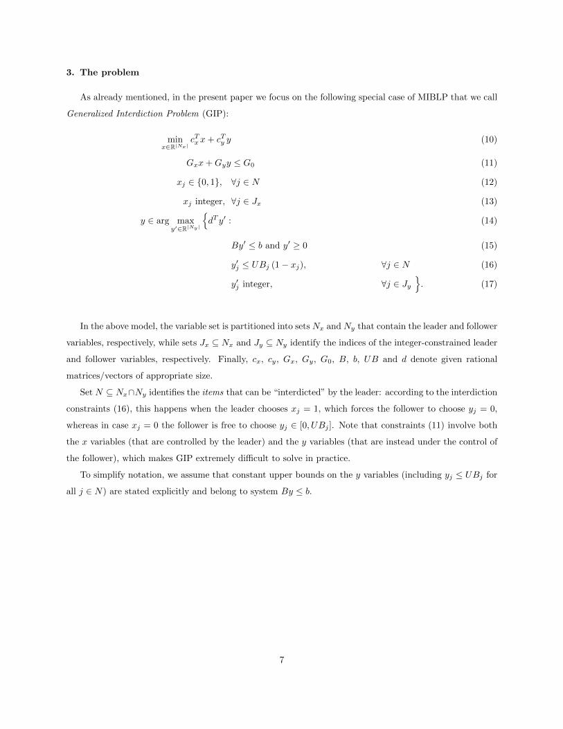
3. The problem

As already mentioned, in the present paper we focus on the following special case of MIBLP that we call

Generalized Interdiction Problem (GIP):

minx∈R|Nx|

cTx x+ cTy y (10)

Gxx+Gyy ≤ G0 (11)

xj ∈ {0, 1}, ∀j ∈ N (12)

xj integer, ∀j ∈ Jx (13)

y ∈ arg maxy′∈R|Ny|

{dT y′ : (14)

By′ ≤ b and y′ ≥ 0 (15)

y′j ≤ UBj (1− xj), ∀j ∈ N (16)

y′j integer, ∀j ∈ Jy}. (17)

In the above model, the variable set is partitioned into sets Nx and Ny that contain the leader and follower

variables, respectively, while sets Jx ⊆ Nx and Jy ⊆ Ny identify the indices of the integer-constrained leader

and follower variables, respectively. Finally, cx, cy, Gx, Gy, G0, B, b, UB and d denote given rational

matrices/vectors of appropriate size.

Set N ⊆ Nx∩Ny identifies the items that can be “interdicted” by the leader: according to the interdiction

constraints (16), this happens when the leader chooses xj = 1, which forces the follower to choose yj = 0,

whereas in case xj = 0 the follower is free to choose yj ∈ [0, UBj ]. Note that constraints (11) involve both

the x variables (that are controlled by the leader) and the y variables (that are instead under the control of

the follower), which makes GIP extremely difficult to solve in practice.

To simplify notation, we assume that constant upper bounds on the y variables (including yj ≤ UBj for

all j ∈ N) are stated explicitly and belong to system By ≤ b.

7

GIP can be restated in its value-function formulation as:

(GIP ) minx,y

cTx x+ cTy y (18)

Gxx+Gyy ≤ G0 (19)

By ≤ b and y ≥ 0 (20)

yj ≤ UBj (1− xj), ∀j ∈ N (21)

dT y ≥ Φ(x) (22)

xj ∈ {0, 1}, ∀j ∈ N (23)

xj integer, ∀j ∈ Jx (24)

yj integer, ∀j ∈ Jy, (25)

where the value function Φ(x) in (22) is computed, for a given x, by solving the follower MILP :

Φ(x) := maxy

{dT y : (20), (21), and (25) hold

}(26)

Thus, unlike general MIBLPs, in the GIP framework the only allowed follower constraints depending on x

are of the form (21).

As customary, we assume that the follower MILP is bounded and feasible for any given x of interest.

In what follows we will rephrase the interdiction constraints (21) in the follower problem through the

bilinear conditions xj yj = 0 for all j ∈ N . As xj and yj are both nonnegative, we can relax these latter

equations in a Lagrangian way through very large positive multipliers Mj (say), and obtain the penalized

objective function

dT y −∑j∈N

Mjxjyj .

This leads to the following reformulation for the follower MILP (26), that we will use throughout:

Φ(x) := maxy

{d(x)T y : (20) and (25) hold

}(27)

where

dj(x) :=

dj −Mjxj , if j ∈ N

dj , otherwise

∀j ∈ Ny. (28)

The above follower reformulation is exact, in the sense that it yields the same value for Φ(x) as the

original formulation (26), provided that each penalty Mj is large enough to impose the implication “xj =

1 =⇒ yj = 0” for all j ∈ N (recall that we assume that the follower problem is feasible and bounded for

each x of interest).

8

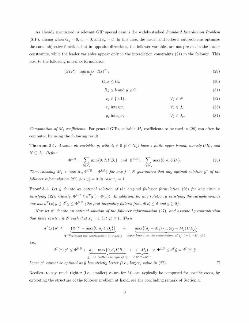
As already mentioned, a relevant GIP special case is the widely-studied Standard Interdiction Problem

(SIP), arising when Gy = 0, cx = 0, and cy = d. In this case, the leader and follower subproblems optimize

the same objective function, but in opposite directions, the follower variables are not present in the leader

constraints, while the leader variables appear only in the interdiction constraints (21) in the follower. This

lead to the following min-max formulation:

(SIP ) minx

maxy

d(x)T y (29)

Gxx ≤ G0 (30)

By ≤ b and y ≥ 0 (31)

xj ∈ {0, 1}, ∀j ∈ N (32)

xj integer, ∀j ∈ Jx (33)

yj integer, ∀j ∈ Jy. (34)

Computation of Mj coefficients. For general GIPs, suitable Mj coefficients to be used in (28) can often be

computed by using the following result.

Theorem 3.1. Assume all variables yi with di 6= 0 (i ∈ Ny) have a finite upper bound, namely UBi, and

N ⊆ Jy. Define

ΦLB :=∑i∈Ny

min{0, di UBi} and ΦUB :=∑i∈Ny

max{0, di UBi}. (35)

Then choosing Mj > max{dj , ΦUB − ΦLB} for any j ∈ N guarantees that any optimal solution y∗ of the

follower reformulation (27) has y∗j = 0 in case xj = 1.

Proof 3.1. Let y denote an optimal solution of the original follower formulation (26) for any given x

satisfying (12). Clearly, ΦLB ≤ dT y (= Φ(x)). In addition, for any solution y satisfying the variable bounds

one has dT (x) y ≤ dT y ≤ ΦUB (the first inequality follows from d(x) ≤ d and y ≥ 0).

Now let y∗ denote an optimal solution of the follower reformulation (27), and assume by contradiction

that there exists j ∈ N such that xj = 1 but y∗j ≥ 1. Then

dT (x) y∗ ≤(ΦUB −max{0, dj UBj}

)︸ ︷︷ ︸ΦUBwithout the contribution of index j

+ max{(dj −Mj) · 1, (dj −Mj)UBj}︸ ︷︷ ︸upper bound on the contribution of y∗j ( = dj−Mj <0 )

i.e.,

dT (x) y∗ ≤ ΦUB + dj −max{0, dj UBj}︸ ︷︷ ︸≤0 no matter the sign of dj

+ (−Mj)︸ ︷︷ ︸<ΦLB−ΦUB

< ΦLB ≤ dT y = dT (x) y

hence y∗ cannot be optimal as y has strictly better (i.e., larger) value in (27). �

Needless to say, much tighter (i.e., smaller) values for Mj can typically be computed for specific cases, by

exploiting the structure of the follower problem at hand; see the concluding remark of Section 4.

9

4. Single-level MILP reformulation

As already stated, the first step of our heuristic consists in relaxing the integrality condition on the y

variables everywhere, namely removing constraints (25) from model (18)-(25) and from model (27). Let GIP

denote the resulting problem, and let SIP be obtained in a similar way from the SIP model (29)-(34) by

dropping (34).

Note that GIP is not a relaxation nor a restriction of the original GIP problem. Indeed, the removal of

the integrality constraints (25) from the follower problem (27) produces the upper bound

Φ(x) := maxy

{d(x)T y : (20) holds

}(36)

on Φ(x), thus increasing the right-hand side of constraint (22). As a consequence, while relaxing the

integrality requirements (25) alone would obviously produce a relaxation of the leader minimization problem

(18)-(25), dropping it in the follower problem makes constraint (22) more restrictive, hence it is impossible

to know if the optimal GIP value is larger or smaller than its counterpart in GIP. (This fact makes it very

difficult to design exact/heuristic solution schemes based on the relaxation of the integrality of the follower

variables.) As a matter of fact, GIP turns out to be a restriction of GIP in case the integrality requirements

(25) in the leader are redundant. This happens, in particular, for the standard interdiction case SIP (where

relaxing the integrality of y makes a broader set of solutions feasible for the follower), hence SIP actually

provides an upper bound on the optimal SIP value. GIP is instead a relaxation of GIP in case the integrality

condition (25) is redundant for the follower. If both cases arise, GIP is just equivalent to the original problem

GIP; this happens, in particular, when Jy = ∅.

We next show how Linear Programming (LP) duality can be used to restate GIP and SIP as single-level

MILPs. Using formulation (36) and standard LP duality, we get

Φ(x) = minu

{uT b : uTB ≥ d(x)T , u ≥ 0

}. (37)

We address SIP first, for which the reformulation is in fact quite natural and can be found, e.g., in

[15, 24, 12, 14].

Theorem 4.1. Model SIP can be restated as

(SIP) minx,u

uT b (38)

Gxx ≤ G0 (39)

xj ∈ {0, 1}, ∀j ∈ N (40)

xj integer, ∀j ∈ Jx (41)

uTB ≥ d(x)T and u ≥ 0. (42)

10

Proof 4.1. Just observe that (38)-(42) can be obtained from (29)-(34) by applying standard LP duality to

the LP relaxation of the inner maximization problem, thus removing the y variables from the model. �

As to GIP, y variables cannot be projected away and thus our formulation involves explicit LP optimality

conditions.

Theorem 4.2. Model GIP can be restated as

(GIP) minx,y,u

cTx x+ cTy y (43)

Gxx+Gyy ≤ G0 (44)

By ≤ b and y ≥ 0 (45)

yj ≤ UBj (1− xj), ∀j ∈ N (46)

xj ∈ {0, 1}, ∀j ∈ N (47)

xj integer, ∀j ∈ Jx (48)

uTB ≥ d(x)T and u ≥ 0 (49)

dT y ≥ uT b. (50)

Proof 4.2. For any given x, primal feasibility of y for the follower LP relaxation (36) comes from (45),

while (49) expresses feasibility of u for its dual (37). According to the strong duality theorem, the pair (y, u)

is then optimal if and only if d(x)T y = uT b, where = can be replaced by ≥ because of weak duality. In

addition, (46)-(47) ensure that d(x)T y = dT y, hence in (50) one is allowed to replace the bilinear condition

d(x)T y ≥ uT b by the equivalent linear constraint dT y ≥ uT b. The claim follows. �

It is worth noting that each constraint in (49) associated with an item j ∈ N has the form

dj − uTBj ≤Mjxj ,

hence it involves a big-M coefficient that can create troubles to the MILP solver. By exploiting the fact that

xj is a binary variable, however, in the relevant case Bj ≥ 0 one has uTBj ≥ 0 and coefficient Mj can safely

be replaced by dj . These (and similar) coefficient strengthenings are automatically applied by modern MILP

solvers and typically produce preprocessed MILP models that, according to our computational experience,

are not too hard to solve.

5. Heuristics

We next describe three heuristics based on the solution of the single-level MILP reformulation (43)-(50)

(for GIP) or (38)-(42) (for SIP) described in the previous section.

11

Our first heuristic, ONE-SHOT, is straightforward to implement, and proved very fast and effective for

many cases in our testbed. For the hardest cases, improved solutions can be obtained by implementing a

more advanced solution scheme. We describe two such schemes.

The first scheme (ITERATE) is also quite easy to implement, and just iterates the application of the

ONE-SHOT heuristic so as to produce diversified solutions.

The second scheme (DYN-REF) requires a more advanced implementation, as valid cuts exploiting the

integrality of the y’s in the follower MILP are dynamically generated and added to the reformulation solved

by ITERATE.

The first two heuristics (ONE-SHOT and ITERATE) can be viewed as a generalization of the solution scheme

described in [12] for KIPs, whereas the third one (DYN-REF) is a new dynamic reformulation heuristic that

makes use, for the first time, of the general-purpose mixed-integer cuts that are automatically generated by

a modern branch-and-cut solver when solving the follower MILP.

5.1. The ONE-SHOT heuristic

Our basic heuristic scheme is described in Algorithms 1 and 2.

Algorithm 1: The refining procedure REFINE(x)

Input : A leader solution x;

Output: A heuristic GIP solution (x, y);

1 Solve the follower MILP (27) for x = x to compute ϕ := Φ(x);

2 Restrict the GIP model (18)-(25) by fixing x = x and by replacing the nonlinear inequality (22) with

the linear constraint dT y ≥ ϕ;

3 Solve the resulting MILP, and let (x, y) be the optimal solution found;

4 return (x, y);

Algorithm 1 describes the refining procedure given, e.g., in [34], that computes a complete feasible GIP

solution (x, y) starting from a leader vector x. It requires the solution of two single-level MILPs: the follower

MILP for x = x at Step 1 to compute Φ(x), and a linearization of the GIP model (18)-(25) based on the fact

that Φ(x) becomes a constant when x is fixed (Steps 2–3). Algorithm 1 typically requires short computing

time, as both MILPs are much easier than the original nonlinear GIP model (see Section 6.4 for details).

Nevertheless, a time limit can be specified in the cases where it is used as a function within a more time

consuming method (such as Algorithm 2 or 3 below), to guarantee that colorblackthe overall run is aborted

within its own time limit. Note that leader variables xj not appearing in the follower MILP (27) (if any),

do not affect the value ϕ = Φ(x) computed at Step 1, hence they need not to be fixed at Step 2.

Algorithm 1 can be simplified for standard interdiction problems. Indeed, in that case Step 3 can be

12

omitted, as the optimal follower solution y computed at Step 1 can directly be appended to the input vector

x to obtain the final solution (x, y) to be returned.

It is worth noting that, for GIPs, the solution (x, y) returned by REFINE, besides being feasible, can have

an improved cost with respect to the (partial) solution provided on input, hence the name of procedure.

Algorithm 2 is used to find a reasonable leader vector, say x, to feed Algorithm 1. This is obtained by

relaxing the integrality of the y variables to be able to apply the single-level MILP reformulation described in

the previous section. The reformulated MILP is typically not too hard to solve, but for very large instances

its exact solution can be too demanding, thus a time limit can be imposed.

Algorithm 2: Our basic ONE-SHOT heuristic scheme

Input : The GIP model (18)-(25);

Output: A heuristic GIP solution (x, y);

1 Relax the integrality of the y variables both in the leader and in the follower problem;

2 Restate the resulting problem as (43)-(50) (GIP) or (38)-(42) (SIP);

3 Solve the resulting single-level MILP (possibly with a time limit), and let (x, ·) be the optimal (or

best) solution found;

4 (x, y) := REFINE(x);

5 return (x, y);

In case at any step of both algorithms the MILP at hand has no feasible solution (or no one could be

found in the given time limit), a void solution (x, y) of cost +∞ is returned.

5.2. The ITERATE heuristic

Our ITERATE heuristic is described in Algorithm 3. At Step 2, a single-level MILP reformulation is

defined; this is either model (43)-(50) (i.e., GIP) or (38)-(42) (i.e., SIP). At each iteration, the single level

reformulation is solved with a time limit, to collect a number of almost-optimal solutions (Step 5). These

solutions coincide, e.g., with the various incumbents by the MILP solver. The refining procedure REFINE is

then applied to each such solution (Step 7). Each time a new heuristic GIP solution (xk, yk) is available, at

Step 9 we possibly update the incumbent (x∗, y∗). When all the available solutions have been refined, the

whole procedure is repeated after adding to the current single-level MILP reformulation a no-good constraint∑j∈N :xk

j =0

xj +∑

j∈N :xkj =1

(1− xj) ≥ 1 (51)

for each generated leader solution xk, thus preventing these solutions to be considered again in subsequent

iterations. Note that, at Step 5, a small part (5%) of the remaining time limit is left for the subsequent

executions of REFINE at Step 7.

13

As to the iterated call to procedure REFINE at Step 7, as already observed, each execution typically

requires very short computing time. Moreover, for SIP one can abort the whole refining procedure for a

given xk as soon as a follower solution of value greater than or equal to z∗ = dT y∗ is encountered. Indeed, for

the follower MILP being a maximization problem, the subsequent part of the REFINE run can only increase

the incumbent cost of the follower, whose best solution, say yk, will produce a heuristic solution (xk, yk) of

cost dT yk ≥ z∗, meaning that the internal incumbent solution (x∗, y∗) will not be updated.

Algorithm 3: The ITERATE heuristic

Input : The GIP model (18)-(25) and a time limit TL;

Output: A heuristic GIP solution (x∗, y∗);

1 Initialize (x∗, y∗) with a dummy solution of cost z∗ := +∞;

2 Build the single-level MILP reformulation (43)-(50) (GIP) or (38)-(42) (SIP);

3 while time limit TL is not exceeded do

4 Let rt be the time remaining to reach the time limit;

5 Solve the current single-level MILP reformulation with a time limit of 0.95 rt, and let

(x1, ·), . . . , (xK , ·) be the collection of solutions found;

6 for k = 1, . . . ,K do

7 (xk, yk) := REFINE(xk);

8 if cTx xk + cTy y

k < z∗ then

9 set z∗ := cTx xk + cTy y

k and (x∗, y∗) := (xk, yk);

10 end

11 Add a no-good constraint (51) for xk to the current single-level MILP reformulation;

12 end

13 end

14 return (x∗, y∗);

We finally observe that our colorblackapproach (though heuristic) is akin to exact method proposed in

[14] for IKP, where specific cuts exploiting the structure of the problem are used—instead of the fully general

no-good constraints (51).

5.3. The DYN-REF heuristic

DYN-REF is our new dynamic reformulation heuristic. It implements an advanced version of ITERATE

where the LP relaxation (36) of the follower MILP formulation (27) is iteratively strengthened by adding

valid inequalities that exploit the integrality of the y variables in the follower problem. In doing so, we aim

at reducing the follower integrality gap, thus hopefully improving the quality of the heuristic solutions found.

14

To this end, observe that the constraints in our follower MILP formulation (27) do not depend on x.

Therefore, after each execution of Step 1 within the refining Algorithm 1, one can just collect the root-node

cuts generated by the MILP solver, and add them to the follower system By ≤ b. The resulting single-level

MILP reformulation solved at Step 5 of Algorithm 3 is thus dynamically updated, and new dual variables

are generated for the newly added rows of (B, b).

Note that, for SIP, the resulting scheme can be interpreted as a dynamic column-generation method where

new columns of BT are added to the SIP reformulation in (42) (to be re-written as BTu ≥ d(x)), while for

GIP we have a row-and-column generation scheme as new rows are also added in (45). A peculiarity of our

scheme is that the generation of the new columns of BT does not require an ad-hoc pricing algorithm, in the

sense that we just re-use the cutting planes generated by the MILP solver invoked with function REFINE.

The generated cuts, besides speeding-up the solution of the next follower MILPs, are very important in

that they hopefully reduce the follower integrality gap and produce a tighter GIP/SIP approximation. In

a sense, our approach is gathering local information obtained by solving the follower MILPs for different

objective functions d(x1)T y, · · · , d(xK)T y within function REFINE, and iteratively incorporates this informa-

tion in the current reformulation to let the heuristic better cope with the consequences of y-integrality at

the follower level.

In this way, we expect a better approximation (hence, hopefully better solutions) at each execution of

the while-loop of Algorithm 3, in particular in the hard cases where the follower formulation has a large

integrality gap. This behavior is in fact confirmed by the computational results reported in the next section.

6. Computational results

In this section we report the outcome of the extensive computational analysis that we performed on a

very large testbed with 1286 instances. Computing times refer to four-thread runs on a quad-core Intel Xeon

E3-1220V2 @3.1 GHz computer with 12GB of RAM.

6.1. Implementation

Our heuristics have been implemented in C, using the commercial solver IBM ILOG CPLEX 12.6.3 as

underlying branch-and-cut framework.

To enhance the performance of Cplex as a heuristic when solving the GIP or SIP reformulation, in our

implementation we switch to the POLISHING [35] heuristic mode after 50% of the imposed time limit. As

to the ITERATE heuristic and its improved version DYN-REF, the collection of K feasible solutions for the

current GIP/SIP reformulation used at Step 5 of Algorithm 3 corresponds to the solutions that are present

in the solution pool of our MILP solver, which contains the various incumbents found during enumeration.

In some versions of our codes, we use the POPULATE feature of Cplex to increase the number of feasible

15

solutions of the reformulation without a very significant increase of the required computing time. To avoid

overtuning, all the other CPLEX parameters (including those related to cut generation) are left at their

default values.

The detailed configurations of the proposed heuristics tested in the computational study are as follows;

the “+” sign in the name of a solver means that the POPULATE feature is active.

• ONE-SHOT (OS): a straightforward implementation of Algorithm 2;

• ONE-SHOT+ (OS+): same as ONE-SHOT, but several solutions of the reformulation are generated by using

POPULATE (and then refined);

• ITERATE (I): a straightforward implementation of Algorithm 3;

• ITERATE+ (I+): same as ITERATE, but several solutions of the reformulation are generated through

POPULATE (and then refined) at each iteration of the while loop;

• DYN-REF+ (DR+): our dynamic reformulation algorithm. This heuristic has the same setting as

ITERATE+, but the Cplex’s root cuts generated during the REFINE procedure are collected and added

to the follower model (and hence to the reformulation through additional dual variables); to avoid

overloading the model, cuts are collected only when the best solution of the current reformulation, say

(x1, ·), is refined.

We also implemented the only general-purpose interdiction heuristic that we could find in the literature,

namely, the greedy algorithm GREEDY (GD) proposed in [3]. This algorithm was designed for standard inter-

diction instances and consists of greedily building an interdiction policy by sorting the items according to

nonincreasing dj ’s (recall that the follower is a maximization problem), and iteratively picking them provided

that the leader constraint Gxx ≤ G0 is fulfilled. For a more fair comparison, we also implemented a simple

4-thread randomized variant GRASP (GR) where alternative interdiction policies are repeatedly created by

following the recipe of GREEDY, but the item which is going to be selected at each iteration is skipped with

a probability of 20%, until the given time limit is reached. In the first iteration of GRASP, we do not do any

skipping, i.e., the solutions of GRASP are always at least as good as those of GREEDY.

6.2. Testbed

In our testbed, we included both standard interdiction problems and generalized interdiction problems. As

to the former, we considered instances from literature, as well as larger versions of some of those instances,

randomly generated following the procedures described in the literature. In particular, the interdiction

problems considered are presented in Section 6.2.1, and consist of the Knapsack Interdiction Problem (KIP),

16

Multidimensional Knapsack Interdiction Problem (MKIP), Clique Interdiction Problem (CIP) and the Fire-

fighter Problem (FFP). Our testbed does not include instead any instance coming, e.g., from network-flow

or shortest-path interdiction problems, as those problems have a continuous follower problem that would

make the MILP reformulation (and hence our heuristic) exact.

Table 1: Our testbed. Column #inst reports the total number of instances in each class. All instances not of type GIP are

standard interdiction instances (Gy = 0, cx = 0, and cy = d). For instances of type KIP and MKIP, there is a one-to-one

correspondence between leader and follower variables, while for the other problems, there are also additional variables in the

follower.

Class Source Type #inst |Nx| |Ny| |N |

CCLW [14] KIP 50 35-55 35-55 35-55

TRSK [22] KIP 150 20-30 20-30 20-30

D [3], [36] KIP 160 10-50 10-50 10-50

LKIP this paper KIP 400 100-500 100-500 100-500

SAC [26] MKIP 144 10-105 10-105 10-105

TRSC [22] CIP 80 19-94 27-109 19-94

TRSC+ this paper CIP 80 19-94 27-109 19-94

LCIP this paper CIP 60 546-1593 586-1653 546-1593

FIRE [37] FFP 72 25-80 50-160 25-80

GEN this paper GIP 90 20-30 20-30 10-30

To the best of our knowledge, there is no previous computational work for generalized interdiction prob-

lems, so we randomly generated a set of GIP instances (denoted by GEN) by using the procedure described

in Section 6.2.2.

Table 1 gives an overview of the instances in our testbed and reports, for each class, the source in the

literature, the associated type of problem, the number of instances and their size. All instances are available

online at https://msinnl.github.io/.

6.2.1. Standard Interdiction Instances

Knapsack and Multidimensional Knapsack Interdiction Problem. The knapsack interdiction problem is de-

fined as follows

minx∈{0,1}|N|

maxy∈{0,1}|N|

{dT y : aTx ≤ a0, q

T y ≤ q0, xj + yj ≤ 1,∀j ∈ N},

where N denotes the set of items.

There are three sets of KIP instances in literature: instance set CCLW from [14], instance set TRSK from

[22], and instance set D from [3] (the latter being derived from multi-objective knapsack instances).

Computational experiments in [26] showed that set CCLW contains the most difficult instances; thus, we

used the same random procedure to create larger random KIP instances denoted by LKIP. The follower data

has been created by using the knapsack instance generator of [38], which allows for generation of the profit

dj and weight qj of each item j ∈ N in the following nine ways, where u.r. stands for uniformly random:

17

1. Uncorrelated: qj u.r. in [1, R], dj u.r. in [1, R].

2. Weakly correlated: qj u.r. in [1, R], dj u.r. in [qj −R/10, qj +R/10] so that dj ≥ 1.

3. Strongly correlated: qj u.r. in [1, R], dj = qj +R/10.

4. Inverse strongly correlated: dj u.r. in [1, R], qj = dj +R/10.

5. Almost strongly correlated: qj u.r. in [1, R], dj u.r. in [qj+R/10−R/500, qj+R/10+R/500].

6. Subset-sum: qj u.r. in [1, R], dj = qj .

7. Even-odd subset-sum: qj even value u.r. in [1, R], dj = qj .

8. Even-odd strongly correlated: qj even value u.r. in [1, R], dj = qj +R/10.

9. Uncorrelated with similar weights: qj u.r. in [100R, 100R+R/10], dj u.r. in [1, R].

In [14], the authors used R = 100 and generated instances of type 1 only. The follower budget is set to

q0 = d INS11

∑j∈N qje, where INS is the number of the instance, with 1 ≤ INS ≤ 10. The leader coefficients

ai are integers chosen u.r. in [0, R], while the leader budget a0 is taken from [q0 − 10, q0 + 10]. All instances

from [14] include at most 55 items. Using the same instance generator, we created larger instances with

|N | ∈ {100, 200, 300, 400, 500}. For each type of instances and number of items, we randomly generated

10 instances. However, instances of type 9 turned out to be trivial as the leader budget allows for the

interdiction of all items, so they have been omitted. Thus, our LKIP testbed includes 400 instances.

MKIP is a generalization of KIP in which the leader and/or the follower have several knapsack con-

straints. For MKIP, a benchmark of 144 instances (set SAC) has been proposed in [26], starting from the 0/1

multidimensional knapsack instances included in the SAC-94 library [39]. In particular, the MKIP instances

were obtained by (i) taking the first constraint as leader constraint, and the remaining ones as follower

constraints; or (ii) considering first half of the constraints as leader constraints, and the remaining ones as

follower constraints; or (iii) considering all but the last constraint as leader constraint.

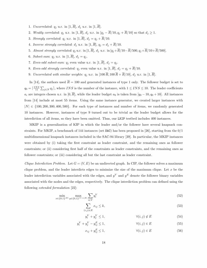
Clique Interdiction Problem. Let G = (V,E) be an undirected graph. In CIP, the follower solves a maximum

clique problem, and the leader interdicts edges to minimize the size of the maximum clique. Let x be the

leader interdiction variables associated with the edges, and yV and yE denote the follower binary variables

associated with the nodes and the edges, respectively. The clique interdiction problem can defined using the

following extended formulation [22]:

minx∈{0,1}|E|

maxy∈{0,1}|V |+|E|

∑i∈V

yVi (52)

∑(i,j)∈E

xij ≤ k, (53)

yVi + yVj ≤ 1, ∀(i, j) 6∈ E (54)

yVi + yVj − yEij ≤ 1, ∀(i, j) ∈ E (55)

xij + yEij ≤ 1, ∀(i, j) ∈ E (56)

18

Set TRSC has been introduced in [22] and is generated in the following way. Graphs are constructed

for graph densities d ∈ {0.7, 0.9} which yields |E| = bd |V | (|V | − 1)/2c. Each potential edge has equal

probability of being created. The interdiction budget k (i.e., the number of edges that can be interdicted)

is chosen as d|E|/4e. Ten instances for each d and |V | ∈ {8, 10, 12, 15} have been created, leading to 80

instances.

To study the influence of the problem formulation on the performance of our heuristics, we also generated

a new set of instances, denoted by TRSC+, that is obtained from TRSC by adding the following redundant

constraints to (52)-(56):

yVi + yVj + yVk − yEij ≤ 1, ∀i, j, k : {i, j} ∈ E, {i, k} 6∈ E, {j, k} 6∈ E. (57)

These constraints are {0, 1/2}-Chvatal-Gomory cuts [40] obtained by combining inequalities (54)-(55), and

are used to strengthen the LP relaxation of the follower formulation which is known to be quite poor.

Moreover, an additional set of larger CIP instances, named LCIP, was generated by using the same

procedure as in TRSK (without the redundant constraints (57)) with |V | ∈ {40, 50, 60}, thus producing 60

new instances.

Firefighter Problem. These instances derive from a trilevel version (following the defender-attacker-defender

scheme of [8]) of the critical node problem recently introduced in [37]. An application of this problem is,

e.g., to stop the spread of wildfire in a forest as well as to limit the effect of malicious viral attacks on a

network. In both cases, given a defender policy, the resulting optimization problem is a bilevel program in

which the leader and the follower operate on a given undirected graph G = (V,E): the leader represents the

malicious player who wants to infect the maximum number of nodes in the network, while the follower tries

to minimize this figure. Both the leader and the follower can select nodes according to some given budget.

In particular, the leader can infect some nodes, from which infection propagates through the edges of the

graph, until it reaches a node that has been protected by the follower. Random instances with number of

nodes |V | ∈ {25, 50, 80} and budget for the leader b up to 5 were generated in [37].

6.2.2. Generalized Interdiction Instances

In this section we describe the procedure we used to randomly generate GIP instances. Observe that, when

no specific structure of the bilevel problem is imposed, one can easily end up with an infeasible or unbounded

instance. Additionally, one may encounter instances for which the optimal solution is unattainable; see, e.g.,

[41, 42] for a discussion of this behavior. A main issue is that, for any given feasible x of the leader, the

follower may be infeasible, resulting in an infeasible problem. Additionally, it may happen that for a given x,

an associated optimal follower solution, say y, is such that (x, y) is not feasible due to the leader constraints

(19).

19

To avoid the pathological cases above, we generated a class GEN of random GIP problems using the

following approach. Instances are constructed by specifying five parameters: number of leader variables

|Nx|, number of follower variables |Ny|, number of interdiction variables |N |, number of leader constraints

|CL| (all in ≤ form), and number of follower constraints |CF | (all in ≤ form). All variables are binary,

and coefficients for the objectives and the constraints are taken uniformly random as integers in [−50, 50].

The right-hand side of each constraint is taken as b α100 · Σc, where α is an integer taken uniformly random

from [25, 75], and Σ is either the sum of all positive or negative coefficients of the currently considered

row (both with 50% probability). Each leader constraint has an additional binary slack x-variable, with

coefficient −100, 000 in the constraint and penalty 100, 000 in the leader objective. This is done to ensure

that, for each x and associated optimal follower solution y, the pair (x, y) is not infeasible due to the leader

constraints (19)—otherwise we many end up with an infeasible instance. Similarly, each follower constraint

has a continuous slack y-variable with coefficient −1 in the constraint, and penalty −100, 000 in the follower

objective. We disregarded all instances for which the HPR did not admit a feasible solution without leader

slack variables. This is done to hopefully obtain instances where the optimal GIP solution does not use

any leader slack variable—though this property cannot be guaranteed, and in fact does not hold for some

generated instances.

We created ten instances for each allowed combination in |Nx| ∈ {20, 30}, |Ny| ∈ {20, 30}, |N | ∈

{10, 20, 30}, and |CL| = |CF | = 20. This resulted in 90 instances (note that the interdiction variables

need to be a subset of the leader/follower variables).

6.3. Results on instances from literature

We first evaluated the performance of our proposed heuristics on the instances from the literature. For

all those instances, the optimal solution value was computed in [4], thus allowing us to evaluate the quality

of the heuristic solutions. Note that, in some cases, the exact method proposed in [4] required one or more

hours of computing time to find a provably optimal solution.

We ran each heuristic algorithm with a very short time limit of just 10 seconds. Table 2 gives the

number of instances for which each algorithm returned an optimal solution (without proving its optimality

of course), as well as the average percentage gap between the heuristic and the optimal solution values. For

each instance, the optimality gap is computed as 100 · |zheu − zopt|/(|zopt| + 10−10), where zheu and zopt

denote the heuristic and optimal solution values, respectively.

The leftmost part of Table 2 refers to the three algorithms (GD, OS, and OS+) that can terminate before the

imposed time limit; as a matter of fact, they were very fast in this test and often required one second or less.

The results in the table show that algorithm OS performs much better than GD: while OS is able to compute

an optimal solution in 65% of the instances and has an average percentage gap of about 17%, GD optimally

solves only 17% of the instances and has an average gap of about 32%. As expected, OS+ has an even (much)

20

Table 2: Results of the heuristics on the instances from the literature, with a time limit of 10 sec.s. Column #opt gives the

number of times a heuristic found the optimal value zopt, and %gap gives the average primal gap, computed as 100 · |zheu −

zopt|/(|zopt|+ 10−10). (∗)Global statistics do not include class TRSC+.

GD OS OS+ GR I I+ DR+

set #inst #opt %gap #opt %gap #opt %gap #opt %gap #opt %gap #opt %gap #opt %gap

CCLW 50 5 17.56 44 0.12 49 0.00 10 6.93 50 0.00 50 0.00 50 0.00

TRSK 150 37 11.79 93 2.00 140 0.35 79 3.82 150 0.00 150 0.00 149 0.08

D 160 58 14.24 154 0.16 160 0.00 115 1.89 160 0.00 160 0.00 160 0.00

SAC 144 7 19.68 121 0.14 136 0.07 30 8.75 142 0.04 141 0.05 143 0.00

TRSC 80 1 98.96 5 73.96 14 44.17 5 70.62 22 37.92 26 29.79 52 14.17

TRSC+ 80 1 98.96 23 36.25 30 26.87 6 69.58 42 20.62 50 14.58 53 12.08

FIRE 72 5 30.43 15 29.69 52 5.68 20 13.27 53 5.67 56 4.24 55 4.58

sum(∗) 656 113 432 551 259 577 583 609

average(∗) 32.11 17.68 8.38 17.55 7.27 5.68 3.14

better performance, in that it is able to compute an optimal solution in 83% of the instances and has an

average gap of about 8%. The rightmost part of the table considers more sophisticated heuristics that run

until the time limit is hit. The randomized version of the greedy (algorithm GR) is clearly the worst method

in this class (only 39% optimal solutions found with an average gap of about 17%), while the other methods

are able to produce an optimal solution for more than 87% of the instances, with an average gap below 7%.

Algorithm DR+ is the clear winner (92% of the instances solved to optimality, with an average error of about

3%), though very good results can be obtained also by using algorithm I+ (88% of the instances solved to

optimality, average error of about 5%).

Observe that the global results in Table 2 (lines “sum” and “average”) do not include instances in class

TRSC+, though the table reports the results for both classes TRSC and TRSC+ to stress the importance of having

a follower formulation with a small integrality gap. As expected, all our heuristics perform significantly better

when the improved formulation is considered, with the only exception of DR+ whose performance is already

quite good even without the additional inequalities (57)—recall that DR+ is able to automatically improve

the follower formulation by generating valid cuts on the fly.

It is worth noting that all our heuristics have an extremely good performance on the first four problem

classes, and a very good one on the last class. For the clique-based instances TRSC, instead, even our best

method (DR+) has an average error of more than 10%. This is partly explained by the fact that the optimal

solution value for these instances typically is a very small integer (less than 5 in most cases), so an error of

just one unit translates into a very large percentage error of 20% or more. A similar consideration applies

(to a lesser extent) to FIRE as well, where the optimal values are small integers in range 2 to 63.

Figure 1 plots the performance profile [43] of the percentage gap of the seven heuristics on the same

instances of Table 2, and confirms the relative ranking among the compared heuristics.

21

Figure 1: Performance profile plot of the percentage gap w.r.t. the optimal solution zopt, computed as 100·|zheu−zopt|/(|zopt|+

10−10), on the instances from the literature, with a time limit of 10 sec.s.

●●●●●●●●●●●●●●●●●●●●●●●●●●●●●●●●●●●●●●●●●●●●●●●●●●●●●●●●●●●●●●●●●●●●●●●●●●●

●●●●●●●●●●●●●●●●●●●●●

●●●●●●●●●●

●●●●●●●●●●●

●●●●●●●●●●●●

●●●● ●●●●●●● ● ●

●●● ● ● ● ● ● ● ●

●●●

70

80

90

100

0 25 50 75 100Primal gap not larger than x%

#in

stan

ces

[%]

Setting● GD

GROSOS+II+DR+

6.4. Results on new instances

In this section we address the newly proposed SIP instances, namely those in sets LKIP and LCIP, as well

as the GIP instances (set GEN). As for these instances the optimal solution value is not known, we evaluated

solution quality by comparison with the value, say zbest, of the best solution found by the heuristics under

comparison. For these instances, all algorithms were executed with a time limit of 60 seconds.

Table 3 reports the outcome of the new experiments. In particular, column “%gap” reports the average

percentage gap with respect to zbest, while column “#bst”gives the number of instances for which the

algorithm produced the best solution. The upper part of the table gives results for SIP instances, whereas

the last line refers to the GIP instances of class GEN. As the benchmark algorithms GD and GR are not designed

for GIP instances, we do not report the associated results in this case. In addition, we do not report the

percentage gap for these instances, as this figure can be extremely large due to the very large objective

coefficient of the slack variables. For setting DR+, we give an additional column “%dgap” that reports the

average percentage dual gap. For each instance, the dual gap is computed as 100·|zDR+−zLB |/(|zDR+|+10−10),

where zDR+ and zLB denote the value of the solution found by DR+ and a lower bound on the optimal GIP/SIP

value, respectively. The lower bound is computed by using the exact solver from [4] for instance sets LCIP

and GEN, and the (more specialized) exact solver from [44] for instance set LKIP. The time limit for the exact

solver was 60 seconds for GEN and LKIP, and 600 seconds for LCIP (to be able to solve at least the root node),

and the reported lower bound is the best among all open nodes.

Figures 2 and 3 plot the performance profile of the percentage gaps computed with respect to zbest for

newly proposed SIP and GIP instances, respectively.

22

Table 3: Results of the heuristics on the new instances, with a time limit of 60 sec.s. Column #bst gives the number of times a

heuristic found the best value zbest, and %gap gives the average primal gap, computed as 100 · |zheu − zbest|/(|zbest|+ 10−10)

for each instance. For instance set GEN the average primal gap is not reported, as it may be very large due to slack variable

coefficients in the objective function. For setting DR+, in column %dgap we also report the average dual gap, computed as

100 · |zDR+ − zLB |/(|zDR+|+ 10−10), where the lower bound zLB is obtained by the (truncated) exact solvers in [4, 44].

GD OS OS+ GR I I+ DR+

set #inst #bst %gap #bst %gap #bst %gap #bst %gap #bst %gap #bst %gap #bst %gap %dgap

LKIP 400 59 20.31 393 0.00 400 0.00 60 19.14 400 0.00 400 0.00 400 0.00 6.28

LCIP 60 0 63.93 0 53.75 34 17.91 0 57.21 1 34.14 40 7.05 58 0.32 76.88

sum 460 59 393 434 60 401 440 458

average 42.12 26.87 8.96 38.17 17.07 3.53 0.16 41.58

GEN 90 - - 24 - 44 - - - 49 - 49 - 90 - 60.17

The results show that all our heuristics perform equally well on LKIP, while for LCIP and GEN our more

advanced version (DR+) has much better performance than all the competing methods. For all instances in

this benchmark too, the greedy algorithm is clearly outperformed by the other heuristics, including the basic

version described in Section 5.1. Finally, observe that algorithm DR+ is consistently the best approach for

GEN instances. As to the dual gap, it is rather large for instance set LCIP due to the poor quality of the lower

bound, while for GEN the gap is not very informative as the big-M coefficients in the objective function can

lead to artificially-large gaps for some instances. For LKIP, instead, the lower bound proved much tighter,

and in fact we report a very good average error of colorblackabout 6% for DR+.

Finally, the experiments confirmed that the runtimes for Steps 1 and 3 in Algorithm 1 (REFINE) are small

compared to the overall runtime: for DR+, Step 1 took on average about 3% of the total computing time,

while Step 3 took on average less than 10% of the total time colorblack(recall that this latter step is not

required for SIP instances).

7. Conclusions and directions of future work

In this paper we have considered Generalized Interdiction Problems (GIPs), a special case of Mixed-

Integer Bilevel Linear Programs (MIBLP) that has important practical applications. Generalized interdiction

can be seen as a Stackelberg game where two players (called the leader and the follower) share a set of items,

and the leader can interdict the usage of certain items by the follower. These problems can be modeled as

Mixed-Integer Nonlinear Programming problems, whose exact solution can be very challenging.

We have proposed a single-level (compact) Mixed-Integer Linear Programming (MILP) reformulation of

the problem obtained from GIP by relaxing the integrality of the follower variables, to be used within a

heuristic solution approach. Three different heuristics of increasing sophistication level have been described

and computationally analyzed on a large set of instances taken from the literature or generated in a random

23

Figure 2: Performance profile plot of the percentage gap w.r.t. the best heuristic solution zbest, computed as 100 · |zheu −

zbest|/(|zbest|+ 10−10), on the instances LCIP and LKIP with a time limit of 60 sec.s.

●●●●●●●●●●●●●●●●●

●●●●●●

●● ●● ●●

● ●●● ● ●●

●● ● ●

●●●

●●

85

90

95

100

0 25 50 75 100Primal gap not larger than x%

#in

stan

ces

[%]

Setting● GD

GROSOS+II+DR+

Figure 3: Performance profile plot of the percentage gap w.r.t. the best heuristic solution zbest, computed as 100 · |zheu −

zbest|/(|zbest|+10−10), on the instance set GEN with a time limit of 60 sec.s. Our DR+ heuristic found the best solution in 100%

of the instences.

●●●●●●●●●●●●●●●●●●●●●●●●●●●●●●●●●●●●● ●●

●●●●●●

●●●●●●●●●●● ● ●●

●●●●●●

40

60

80

100

0 25 50 75 100Primal gap not larger than x%

#in

stan

ces

[%] Setting

● OSOS+II+DR+

way. In particular, our new dynamic reformulation heuristic uses a mathematically-sound way to bring

integrality information (in the form of valid cuts) from the follower to the global level. The outcome of

our experiments is that even the simplest reformulation heuristic works well on a large number of the

tested instances, often providing an optimal solution within negligible computing time. For the hardest

cases, however, our new dynamic reformulation heuristic produces significantly improved results and clearly

24

outperforms all compared methods.

An interesting research topic is how to use our heuristics within an exact (enumerative) solution method.

Indeed, while the use of any initial heuristic to produce a warm-start incumbent is clearly straightforward,

the definition of a sound integration scheme is more challenging, as the heuristics must be invoked at the

enumeration nodes (thus taking advantage of the local information therein available) but do not have to

introduce an excessive overhead. This topic is outside the scope of the present paper (which concentrates on

the analysis of stand-alone heuristics) and is left to future research.

Future research should also address the application of our dynamic reformulation heuristic scheme to

other min-max problems such as those arising in min-max regret robustness, as well as to problems where

interdiction penalties are considered as, e.g., in [15]. Another interesting line of research is the application of

similar heuristic schemes to general MIBLPs. Also in this context, dropping the integrality requirement on

the follower variables leads to a single-level MILP reformulation, so our heuristic approach can be applied

with only minor adaptations. In the general bilevel case, however, the single-level reformulation is based on

KKT conditions, hence it implies hard disjunctive constraints that can make its resolution quite problematic

in practice. As a matter of fact, preliminary computational results show that the bilevel heuristic performs

well for some instances, but additional research effort is needed to reduce the solution time of the single-level

MILP reformulation.

Acknowledgment

This research was funded by the Vienna Science and Technology Fund (WWTF) through project ICT15-

014. The work of the first two authors was also supported MiUR, Italy (PRIN project), while that of the

last author was also supported by the Austrian Research Fund (FWF, Project P 26755-N19). Thanks are

due to the anonymous referees for their constructive comments.

References

[1] P. Loridan, J. Morgan, Weak via strong Stackelberg problem: new results, Journal of Global Optimiza-

tion 8 (1996) 263–297.

[2] J. Outrata, On the numerical solution of a class of Stackelberg problems, ZOR - Methods and Models

of Operations Research 34 (1990) 255–277.

[3] S. DeNegre, Interdiction and discrete bilevel linear programming, Ph.D. thesis, Lehigh University (2011).

[4] M. Fischetti, I. Ljubic, M. Monaci, M. Sinnl, A new general-purpose algorithm for mixed-integer bilevel

linear programs, Operations Research (2017) (to appear).

25

[5] H. Von Stackelberg, The theory of the market economy, Oxford University Press, 1952.

[6] E. Israel, System interdiction and defense, Ph.D. thesis, Monterey, California: Naval Postgraduate

School (1999).

[7] G. Brown, M. Carlyle, J. Salmeron, K. Wood, Analyzing the vulnerability of critical infrastructure

to attack and planning defenses, Tutorials in Operations Research: Emerging Theory, Methods, and

Applications (2005) 102–123.

[8] G. Brown, M. Carlyle, J. Salmeron, K. Wood, Defending critical infrastructure, Interfaces 36 (6) (2006)

530–544.

[9] A. Washburn, K. Wood, Two-person zero-sum games for network interdiction, Operations Research

43 (2) (1995) 243–251.

[10] G. Brown, M. Carlyle, R. Harney, E. Skroch, K. Wood, Interdicting a nuclear-weapons project, Opera-

tions Research 57 (4) (2009) 866–877.

[11] D. P. Morton, F. Pan, K. J. Saeger, Models for nuclear smuggling interdiction, IIE Transactions 39 (1)

(2007) 3–14.

[12] A. Lodi, T. Ralphs, F. Rossi, S. Smriglio, Interdiction branching, Technical Report, COR@L Laboratory,

Lehigh University (2011).

[13] A. Lodi, T. K. Ralphs, G. J. Woeginger, Bilevel programming and the separation problem, Math.

Program. 146 (1-2) (2014) 437–458.

[14] A. Caprara, M. Carvalho, A. Lodi, G. Woeginger, Bilevel knapsack with interdiction constraints, IN-

FORMS Journal on Computing 28 (2) (2016) 319–333.

[15] E. Israeli, R. Wood, Shortest-path network interdiction, Networks 40 (2) (2002) 97–111.

[16] C. Lim, J. C. Smith, Algorithms for discrete and continuous multicommodity flow network interdiction

problems, IIE Transactions 39 (1) (2007) 15–26.

[17] R. K. Wood, Deterministic network interdiction, Mathematical and Computer Modelling 17 (2) (1993)

1–18.

[18] F. Furini, M. Iori, S. Martello, M. Yagiura, Heuristic and exact algorithms for the interval min–max

regret knapsack problem, INFORMS Journal on Computing 27 (2) (2015) 392–405.

26

[19] L. Assuncao, T. F. Noronha, A. C. Santos, R. Andrade, A linear programming based heuristic framework

for min-max regret combinatorial optimization problems with interval costs, Computers & Operations

Research 81 (2017) 51–66.

[20] C. Bazgan, S. Toubaline, D. Vanderpooten, Efficient determination of the k most vital edges for the

minimum spanning tree problem, Computers & Operations Research 39 (11) (2012) 2888–2898.

[21] D. R. Fulkerson, G. C. Harding, Maximizing the minimum source-sink path subject to a budget con-

straint, Mathematical Programming 13 (1) (1977) 116–118.

[22] Y. Tang, J.-P. Richard, J. Smith, A class of algorithms for mixed-integer bilevel min–max optimization,

Journal of Global Optimization (2015) 1–38.

[23] A. Caprara, M. Carvalho, A. Lodi, G. J. Woeginger, A study on the computational complexity of the

bilevel knapsack problem, SIAM Journal on Optimization 24 (2) (2014) 823–838.

[24] R. Wood, Bilevel Network Interdiction Models: Formulations and Solutions, John Wiley & Sons, Inc.,

2010.

[25] C. Bazgan, S. Toubaline, Z. Tuza, The most vital nodes with respect to independent set and vertex

cover, Discrete Applied Mathematics 159 (17) (2011) 1933 – 1946.

[26] M. Fischetti, I. Ljubic, M. Monaci, M. Sinnl, Interdiction games and monotonicity, Technical Report,

DEI, University of Padova (2016).

[27] H. Held, D. L. Woodruff, Heuristics for multi-stage interdiction of stochastic networks, Journal of

Heuristics 11 (2005) 483–500.

[28] M. Gendreau, P. Marcotte, G. Savard, A hybrid tabu-ascent algorithm for the linear bilevel programming

problem, Journal of Global Optimization 8 (3) (1996) 217–233.

[29] C. Audet, J. Haddad, G. Savard, Disjunctive cuts for continuous linear bilevel programming, Optimiza-

tion Letters 1 (3) (2007) 259–267.

[30] S. Dempe, A simple algorithm for the linear bilevel programming problem, Optimization 18 (1987)

373–385.

[31] U. P. Wen, A. D. Huang, A simple tabu search method to solve the mixed-integer linear bilevel pro-

gramming problem, European Journal of Operational Research 88 (3) (1996) 563–571.

[32] H. I. Calvete, C. Gal, P. M. Mateo, A new approach for solving linear bilevel problems using genetic

algorithms, European Journal of Operational Research 188 (1) (2008) 14–28.

27

[33] E.-G. Talbi, Metaheuristics for bi-level optimization, Vol. 482, Springer, 2013.

[34] M. Fischetti, I. Ljubic, M. Monaci, M. Sinnl, Intersection cuts for bilevel optimization, in: Q. Lou-

veaux, M. Skutella (Eds.), Integer Programming and Combinatorial Optimization: 18th International

Conference, IPCO 2016, Liege, Belgium, June 1-3, 2016, Proceedings, Springer International Publish-

ing, Extended version submitted for publication, 2016, pp. 77–88.

URL http://www.dei.unipd.it/~fisch/papers/intersection_cuts_for_bilevel_optimization.

pdf

[35] E. Rothberg, An evolutionary algorithm for polishing mixed integer programming solutions, INFORMS

Journal on Computing 19 (4) (2007) 534–541.

[36] T. K. Ralphs, E. Adams, Bilevel instance library, http://coral.ise.lehigh.edu/data-sets/

bilevel-instances/ (2016).

[37] A. Baggio, M. Carvalho, A. Lodi, A. Tramontani, Multilevel approaches for the critical node problem,

working paper, Ecole Polytechnique de Montreal (2016).

[38] S. Martello, D. Pisinger, P. Toth, Dynamic programming and strong bounds for the 0-1 knapsack

problem, Management Science 45 (3) (1999) 414–424.

[39] S. Khuri, T. Baeck, J. Heitkoetter, SAC94 Suite: Collection of Multiple Knapsack Problems, http:

//www.cs.cmu.edu/Groups/AI/areas/genetic/ga/test/sac/0.html (1994).

[40] A. Caprara, M. Fischetti, {0, 1/2}-Chvatal-Gomory cuts, Mathematical Programming 74 (3) (1996)

221–235.

[41] J. Moore, J. Bard, The mixed integer linear bilevel programming problem, Operations Research 38 (5)

(1990) 911–921.

[42] M. Koppe, M. Queyranne, C. T. Ryan, Parametric integer programming algorithm for bilevel mixed

integer programs, Journal of Optimization Theory and Applications 146 (1) (2010) 137–150.

[43] E. D. Dolan, J. More, Benchmarking optimization software with performance profiles, Mathematical

programming 91 (2) (2002) 201–213.

[44] M. Fischetti, I. Ljubic, M. Monaci, M. Sinnl, Interdiction games and monotonicity, technical report.

28