Real-Time Operating Systems

10EC842

Prepared by: Shivanand Gowda KR

Dept of ECE

Alpha College of Engineering

Introduction to Real-Time Embedded Systems

The concept of real time digital computing systems is an emergent concept

compared to most engineering theory and practice. When requested to complete a

task or provide a service in real time , the common understanding is that this task

must be done upon request and completed while the requester waits for the

completion as an output response; If the response to the request is too slow, the

requestor may consider lack of response a failure. More specifically it constitutes

a real time service request indicate a real world event sensed by the system. For

example, a new video frame has been digitized and placed in memory for

processing. The computing platform must now process input related to the service

request and produce an output response prior to a deadline measured relative to an

event sensed earlier. The real time digital computing system must produce a

response upon request while the user and/ or system wait. After the deadline

established for the response, relative to the request time, the user gives up or the

system fails to meet requirements if no response has been produced.

A common way to define real time as a noun is the time during which a process

takes place or occurs. Used as an adjective, real time relates to computer

applications or processes that can respond with low bounded latency to user

requests.

Definition of embedding is helpful for understanding what is meant by a real time

embedded system. Embedding means to enclose or implant as essential or

characteristic. From the viewpoint of computing systems, an embedded system is a

special purpose computer completely contained within the device it controls and

not directly observable by the user of the system.

A BRIEF HISTORY OF REAL TIME SYSTEMS

The origin of real time comes from the recent history of process control

using digital computing platforms. In fact, an early definitive text on the concept

was published in 1965 [Martin65]. The concept of real time is also rooted in

computer simulation, where a simulation that runs at least as fast as the real world

physical process it models is said to run in real time.

Liu and Layland also defined the concept of soft real time in 1973, however there

is still no universally accepted formal definition of soft real time. The concept of

hard real time systems became better understood based upon experience and

problems noticed with fielded systems one of the most famous examples early on

was the Apollo 11 lunar module descent guidance overload. The Apollo 11 system

suffered CPU resource overload that threatened to cause descent guidance services

to miss deadlines and almost resulted in aborting the first landing on the moon.

During descent of the lunar module and use of the radar system, astronaut Buzz

Aldrin notes a computer guidance system alarm.

A BRIEF HISTORY OF EMBEDDED SYSTEMS

Embedding is a much older concept than real time. Embedded digital

computing systems are often an essential part of any real time embedded system

and process sensed input to produce responses as output to actuators. The sensors

and actuators are components providing I/O and define the interface between an

embedded system and the rest of the system or application. Left with this as the

definition of an embedded digital computer, you could argue that a general purpose

workstation is an embedded system; after all, a mouse, keyboard, and video display

provide sensor/actuator driven between the digital computer and a user. However,

to satisfy the definition of an embedded system better, we distinguish the types of

services provided. A general purpose work station provides a platform for

unspecified to be determined sets of services, whereas an embedded system

provides a well defined service or set of services such as anti locking control. In

general, providing general services is impractical for applications such as

computation of 1c to the nth digit, payroll, or office automation on an embedded

system. Finally, the point of an embedded system is to cost effectiveness, a more

limited set of services in a larger system, such as an automobile, aircraft, or

telecommunications switching center.

Real-Time Services

The concept of a real time service is fundamental in real time embedded

systems. Conceptually, a real time service provides a transformation of inputs to

outputs in A an embedded system to provide a function.For example, a service

might provide thermal control for a subsystem by sensing temperature with

thermisters (temperature sensitive resistors) to cool the subsystem with a fan or to

heat it with electric coils. The service provided in this example is thermal

management such that the subsystem temperature is maintained within a set range.

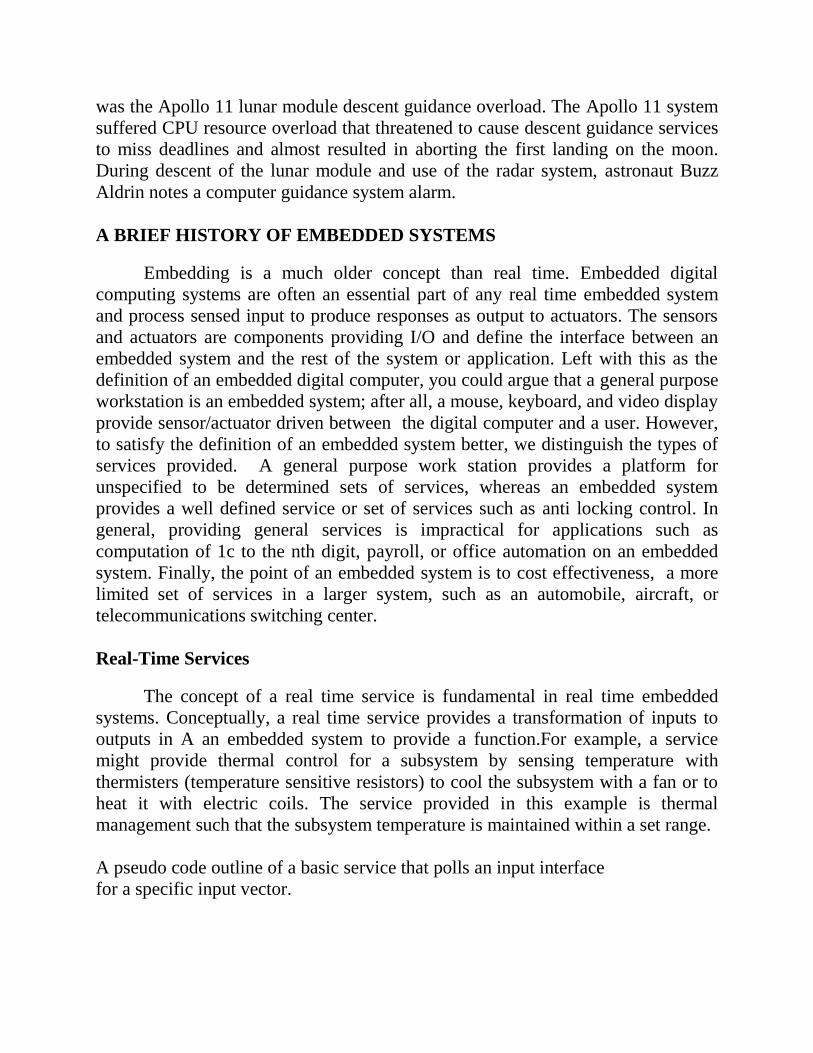
A pseudo code outline of a basic service that polls an input interface

for a specific input vector.

When a software implementation is used for multiple services on a single CPU,

software polling is often replaced with hardware offload of the event detection and

input encoding. The offload is most often done with an ADC (Analog to Digital

Converter) and DMA (Direct Memory Access) engine that implements the Event

Sensing state in Figure. This hardware state machine then asserts an interrupt

input into the CPU, which in turn sets a flag used by a scheduling state machine to

indicate that a software data processing service should be dispatched for execution.

The following is a pseudo code outline of a basic event driven software service.

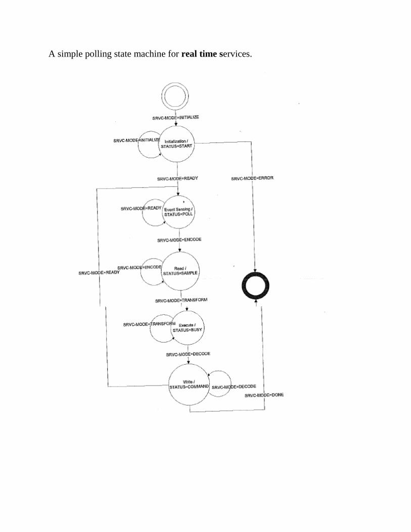
A simple polling state machine for real time services.

Realtime digital control and process control services are periodic by nature. The

system either polls sensors on a periodic basis, or the sensor components provide

digitized data on a known sampling interval with an interrupt generated to the

controller. The periodic services in digital control systems implement the control

law of a digital control system. When a microprocessor is dedicated to only one

service, the design and implementation of services is fairly simple.

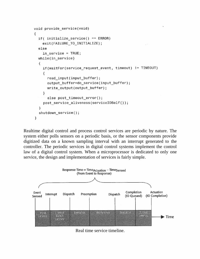
Real time service timeline.

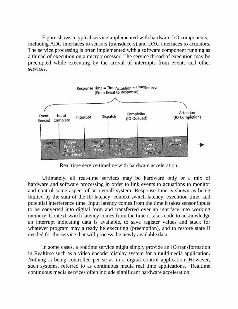
Figure shows a typical service implemented with hardware I/O components,

including ADC interfaces to sensors (transducers) and DAC interfaces to actuators.

The service processing is often implemented with a software component running as

a thread of execution on a microprocessor. The service thread of execution may be

preempted while executing by the arrival of interrupts from events and other

services.

Real time service timeline with hardware acceleration.

Ultimately, all real-time services may be hardware only or a mix of

hardware and software processing in order to link events to actuations to monitor

and control some aspect of an overall system. Response time is shown as being

limited by the sum of the IO latency, context switch latency, execution time, and

potential interference time. Input latency comes from the time it takes sensor inputs

to be converted into digital form and transferred over an interface into working

memory. Context switch latency comes from the time it takes code to acknowledge

an interrupt indicating data is available, to save register values and stack for

whatever program may already be executing (preemption), and to restore state if

needed for the service that will process the newly available data.

In some cases, a realtime service might simply provide an IO transformation

in Realtime such as a video encoder display system for a multimedia application.

Nothing is being controlled per se as in a digital control application. However,

such systems, referred to as continuous media real time applications, Realtime

continuous media services often include significant hardware acceleration.

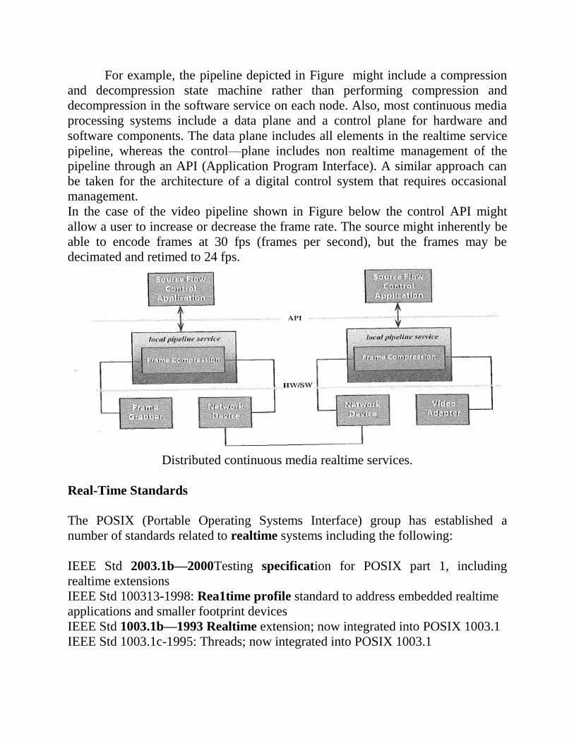
For example, the pipeline depicted in Figure might include a compression

and decompression state machine rather than performing compression and

decompression in the software service on each node. Also, most continuous media

processing systems include a data plane and a control plane for hardware and

software components. The data plane includes all elements in the realtime service

pipeline, whereas the control—plane includes non realtime management of the

pipeline through an API (Application Program Interface). A similar approach can

be taken for the architecture of a digital control system that requires occasional

management.

In the case of the video pipeline shown in Figure below the control API might

allow a user to increase or decrease the frame rate. The source might inherently be

able to encode frames at 30 fps (frames per second), but the frames may be

decimated and retimed to 24 fps.

Distributed continuous media realtime services.

Real-Time Standards

The POSIX (Portable Operating Systems Interface) group has established a

number of standards related to realtime systems including the following:

IEEE Std 2003.1b—2000Testing specification for POSIX part 1, including

realtime extensions

IEEE Std 100313-1998: Rea1time profile standard to address embedded realtime

applications and smaller footprint devices

IEEE Std 1003.1b—1993 Realtime extension; now integrated into POSIX 1003.1

IEEE Std 1003.1c-1995: Threads; now integrated into POSIX 1003.1

IEEE Std 1003.1d—1Ad9di9tio9na:l real time extensions; now integrated into

POSIX 1003.1—2001which was later replaced by POSIX 1003.1—2003

IEEE Std 1003.1j—20A0dv0an:ced real—time extensions; now integrated into

POSIX 10031-2001, which was later replaced by POSIX 1003.1—2003

IEEE Std 1003.1q-2000: Tracing

The most significant standard for realtime systems from POSIX is 1003.1b,

which specifies the API that most ARTOS(Real Time Operating Systems) and

realtime.

Linux operating systems implement. The POSIX 1003.1b extensions include

Definitions of the following real—time operating system mechanisms:

Priority Scheduling

Real Time Signals

Clocks and Timers

Semaphores

Message Passing

Shared Memory

Asynchronous and Synchronous I/ O

Memory Locking

System Resources

Introduction

Resource Analysis

Real Time Service Utility

Scheduling Classes

The Cyclic Executive

Scheduler Concepts

Real Time Operating Systems

Thread Safe Functions

INTRODUCTION

Real time embedded systems must provide deterministic behavior and often have more

rigorous time and safety critical system requirements compared to general purpose desktop

computing systems. For example, a satellite real time embedded system must survive launch and

the space environment, must be very efficient in terms of power and mass, and must meet high

reliability standards. Applications that provide a real time service could in some cases be much

simpler if they were not resource constrained by system requirements typical of an embedded

environment. The engineer must instead carefully consider resource limitations, including power,

mass, size, memory capacity, processing, and I/O bandwidth. Furthermore, complications of

reliable operation in hazardous environments may require specialized resources such as error

detecting and correcting memory systems. To successfully implement real time services in a

system providing embedded functions, resource analysis must be completed to ensure that these

services are not only functionally correct, but that they produce output on time and with high

reliability and availability.

The three fundamental resources, CPU, memory, and I/O, are excellent places to start

understanding the architecture of real time embedded systems and how to meet design

requirements and objectives. Furthermore, resource analysis is critical to the hardware, firmware,

and software design in a real time embedded system.

RESOURCE ANALYSIS

There are common resources that must be sized and managed in any real time embedded system

including the following:

Processing: Any number of microprocessors or microcontrollers networked together.

Memory: All storage elements in the system including volatile and nonvolatile storage.

I/O: Input and output that encodes sensed data and is used for decoding for actuation.

Traditionally the main focus of real time resource analysis and theory has been centered around

processing and how to schedule multiplexed execution of multiple services on a single processor.

Scheduling resource usage requires the system software to make a decision to allocate a resource

such as the CPU to a specific thread of execution. The mechanics of multiplexing the CPU by

preempting a running thread, saving its state, and dispatching a new thread is called a thread

context switch. Scheduling involves implementing a policy, whereas preemption and dispatch

are context switching. When a CPU is multiplexed with an RTOS scheduler and context

switching, the system architect must determine whether the CPU resources are sufficient given

the set of service threads to be executed and whether the services will be able to reliably

complete execution prior to system required deadlines.

The main considerations include speed or instruction execution (clock rate), the efficiency of

executing instructions (average Clocks Per Instruction [CPI]), algorithm complexity, and

frequency of service requests.

Speed: Clock Rate for Instruction Execution.

Efficiency: CPI or IPC (Instructions Per Clock); processing stalls due to hazards; for example,

read data dependency, cache misses, and write buffer overflow stalls.

Algorithm complexity: Ci = instruction count on service longest path for service i and ideally,

is deterministic; if Ci - is not known, the worst case should be used WCET (Worst Case

Execution Time) is the longest, most inefficiently executed path for service; WCET is one

component of response time ); other contributions to response time come from input latency;

dispatch latency; execution; interference by higher priority services and interrupts and output

latency.

Service Frequency: Ti = Service Release Period.

Input and output channels between processor cores and devices are one of the most

important resources in real time embedded systems and perhaps one of the most often

overlooked as far as theory and analysis. In a real time embedded system, low latency for I/O is

fundamental. The response time of a service can be highly influenced by I/O latency.

Furthermore, no response is complete until writes actually drain to output device interfaces. So,

key I/O parameters are latency, bandwidth, read/write queue depths, and coupling between I/ O

channels and the CPU.

Latency

Arbitration latency for shared I/O interfaces

Read latency

Time for data transit from device to CPU core

Registers, Tightly Coupled Memory (TCM), and L1 cache for zero wait state single cycle

access

Bus interface read requests and completions: split transactions and delay

Write latency

Time for data transit from CPU core to device.

Posted writes prevent CPU stalls

Posted writes require bus interface queue

Bandwidth (BW)

Average bytes or words transferred per unit time

BW says nothing about latency, so it is not a panacea for real time systems

Queue depth

Write buffer stalls will decrease efficiency when queues fill up

Read buffers most often stalled by need for data to process

CPU coupling

DMA channels help decouple the CPU from I/O

Programmed I/ O strongly couples the CPU to I/O

Cycle stealing requires occasional interaction between the CPU and DMA engines

Memory resources are designed based upon cost, capacity, and access latency. Ideally all

memory would be zero wait state so that the processing elements in the system could access data

in a single processing cycle. Due to cost, the memory is most often designed as a hierarchy with

the fastest memory being the smallest due to high cost, and large capacity memory the largest

and lowest cost per unit storage. Nonvolatile memory is most often the slowest access.

Memory hierarchy from least to most latency

Level-1cache

Single cycle access

Typically Harvard architecture separate data and instruction caches.

Locked for use as fast memory, unlocked for set associative or direct mapped caches.

Level-2 cache or TCM

Few or no wait states (e.g., 2 cycle access)

Typically unified (contains both data and code)

Locked for use as TCM, unlocked to back Ll caches

MMRs (Memory Mapped Registers)

Main memory SRAM,SDRAM, DDR

Processor bus interface and controller

Multicycle access latency on chip

Many cycle latency off chip

MMIO (Memory Mapped I/O) Devices

Non volatile memory like flash, EEPROM, and battery backed SRAM

Slowest read/write access, most often off chip.

Requires algorithm for block erase and interrupt upon completion and poll

for completion for flash and EEPROM

Total capacity for code, data, stack, and heap requires careful planning.

Allocation of data, code, stack, heap to physical hierarchy will significantly affect performance.

Real time theory and systems design have focused almost entirely on sharing CPU resources and

to a lesser extent, issues related to shared memory, I/O latency, I/O scheduling, and

synchronization of services.

A given system may experience problems meeting service deadlines because it is:

CPU bound: Insufficient execution cycles during release period and due to inefficiency in

Execution.

I/O bound: Too much total I/O latency during the release period and/ or poor scheduling of I/O

during execution.

Memory bound: Insufficient memory capacity or too much memory access latency during the

release period.

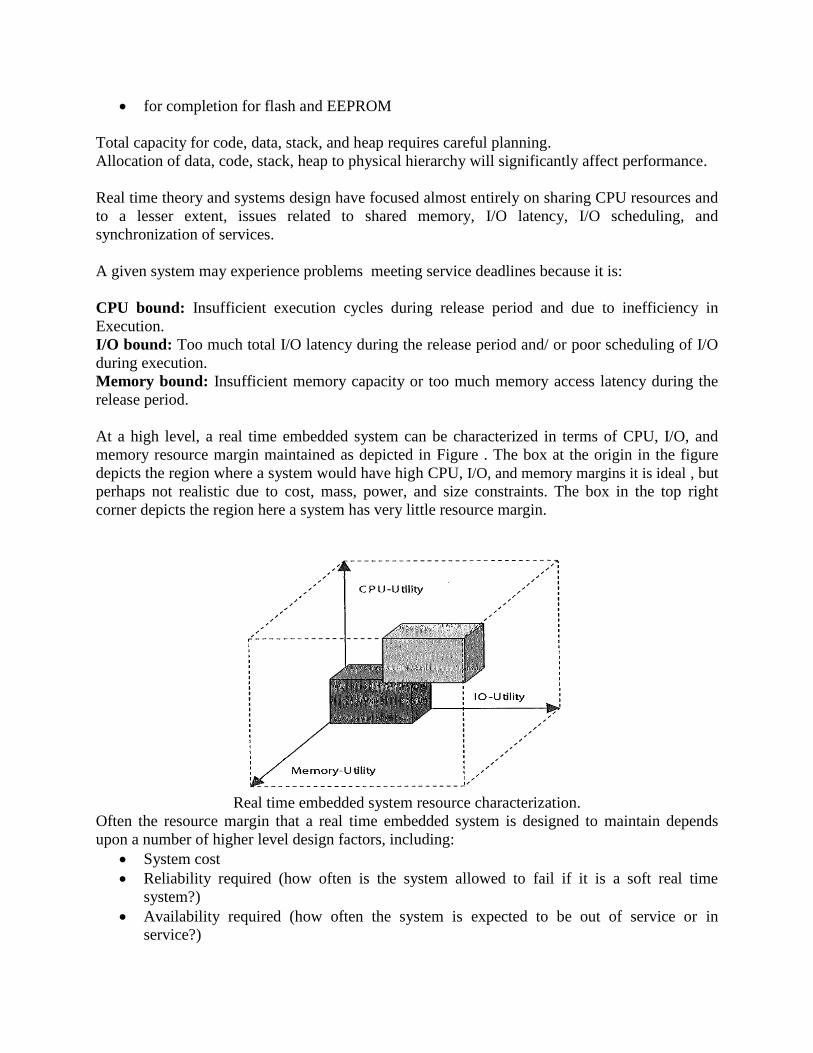
At a high level, a real time embedded system can be characterized in terms of CPU, I/O, and

memory resource margin maintained as depicted in Figure . The box at the origin in the figure

depicts the region where a system would have high CPU, I/O, and memory margins it is ideal , but

perhaps not realistic due to cost, mass, power, and size constraints. The box in the top right

corner depicts the region here a system has very little resource margin.

Real time embedded system resource characterization.

Often the resource margin that a real time embedded system is designed to maintain depends

upon a number of higher level design factors, including:

System cost

Reliability required (how often is the system allowed to fail if it is a soft real time

system?)

Availability required (how often the system is expected to be out of service or in

service?)

Risk of over subscribing resources (how deterministic are resource demands?)

Impact of over subscription (if resource margin is insufficient, what are the

consequences?)

Prescribing general margins for any system with specific values is difficult. However, here are

some basic guidelines for resource sizing and margin maintenance:

CPU: The set of proposed services must be allocated to processors so that each processor in the

system meets the Lehoczky,Shah, Ding theorem for feasibility. Normally, the CPU margin

required is less than the RM LUB (Rate Monotonic Least Upper Bound) of approximately 30%.

The amount of margin required depends upon the service parameters mostly their relative release

periods and how harmonic the periods are.

I/O: Total I/O latency for a given service should never exceed the response deadline or the

service release period (often the deadline and period are the same). Overlapping I/O time with

execution time is therefore a key concept for better performance. Scheduling I/O so that it is

overlaps is often called I/O latency hiding.

Memory: The total memory capacity should be sufficient for the worst case static and dynamic

memory requirements for all services. Furthermore, the memory access latency summed with the

I/O latency should not exceed the service release period. Memory latency can be hidden by

overlapping memory latency with careful instruction scheduling and use of cache to improve

performance.

The largest challenge in real time embedded systems is dealing with the tradeoff between

determinism and efficiency gained from less deterministic architectural features such as set

associative caches and overlapped I/O and execution. For hard real time systems where the

consequences of failure are too severe to ever allow, the worst case must always be assumed. For

soft real time systems, a better trade off can be made to get higher performance for lower cost,

but with higher probability if occasional service failures.

In the worst case, the response time equation is

All services Si in a hard real time system must have response times less than their required

deadline, and the response time must be assumed to be the sum of the total worst case latency.

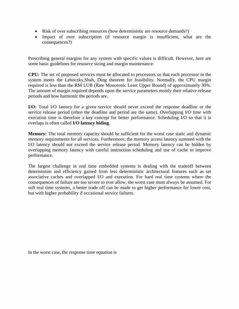
REAL-TIME SERVICE UTILITY

To more formally describe various types of real time services, the real time research community

devised the concept of a service utility function. The service utility function for a simple real

time service is depicted in Figure below. The service is said to be released when the service is

ready to start execution following a service request, most often initiated by an interrupt. The

utility of the service producing a response any time prior to the deadline relative to the request is

full, and at the instant following the deadline, the utility not only becomes zero, but actually

negative.

Hard real time service utility

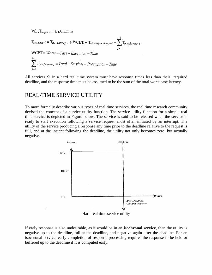
If early response is also undesirable, as it would be in an isochronal service, then the utility is

negative up to the deadline, full at the deadline, and negative again after the deadline. For an

isochronal service, early completion of response processing requires the response to be held or

buffered up to the deadline if it is computed early.

Isochronal service utility

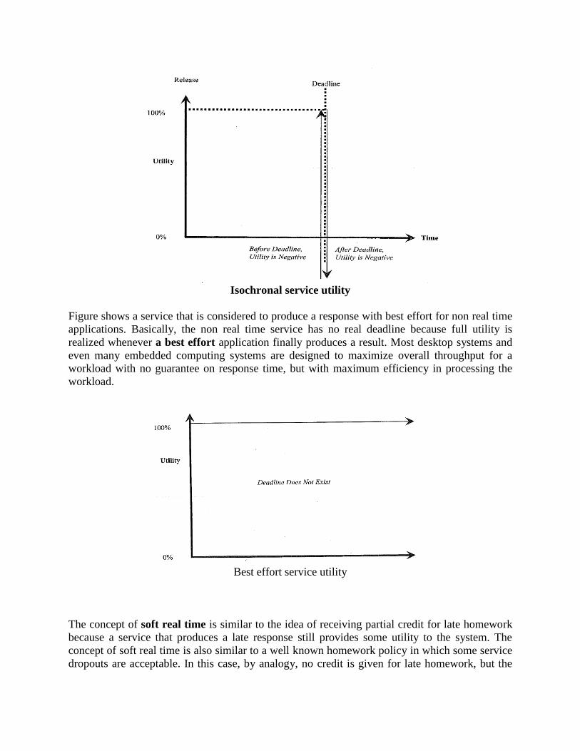
Figure shows a service that is considered to produce a response with best effort for non real time

applications. Basically, the non real time service has no real deadline because full utility is

realized whenever a best effort application finally produces a result. Most desktop systems and

even many embedded computing systems are designed to maximize overall throughput for a

workload with no guarantee on response time, but with maximum efficiency in processing the

workload.

Best effort service utility

The concept of soft real time is similar to the idea of receiving partial credit for late homework

because a service that produces a late response still provides some utility to the system. The

concept of soft real time is also similar to a well known homework policy in which some service

dropouts are acceptable. In this case, by analogy, no credit is given for late homework, but the

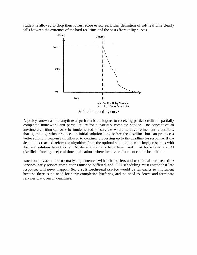
student is allowed to drop their lowest score or scores. Either definition of soft real time clearly

falls between the extremes of the hard real time and the best effort utility curves.

Soft real time utility curve

A policy known as the anytime algorithm is analogous to receiving partial credit for partially

completed homework and partial utility for a partially complete service. The concept of an

anytime algorithm can only be implemented for services where iterative refinement is possible,

that is, the algorithm produces an initial solution long before the deadline, but can produce a

better solution (response) if allowed to continue processing up to the deadline for response. If the

deadline is reached before the algorithm finds the optimal solution, then it simply responds with

the best solution found so far. Anytime algorithms have been used most for robotic and AI

(Artificial Intelligence) real time applications where iterative refinement can be beneficial.

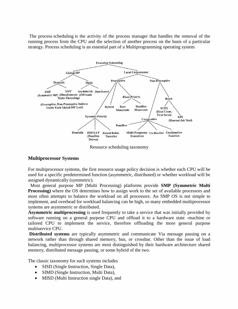
Isochronal systems are normally implemented with hold buffers and traditional hard real time

services, early service completions must be buffered, and CPU scheduling must ensure that late

responses will never happen. So, a soft isochronal service would be far easier to implement

because there is no need for early completion buffering and no need to detect and terminate

services that overrun deadlines.

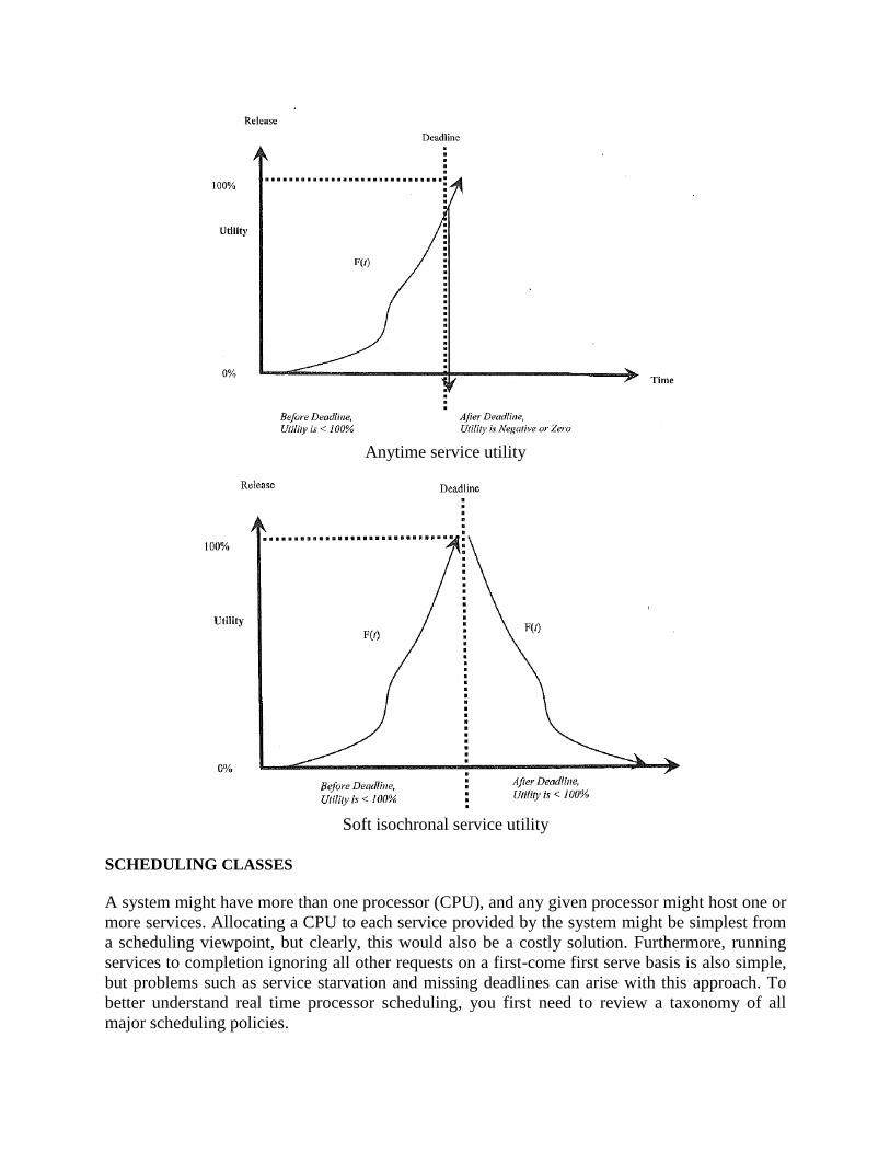
Anytime service utility

Soft isochronal service utility

SCHEDULING CLASSES

A system might have more than one processor (CPU), and any given processor might host one or

more services. Allocating a CPU to each service provided by the system might be simplest from

a scheduling viewpoint, but clearly, this would also be a costly solution. Furthermore, running

services to completion ignoring all other requests on a first-come first serve basis is also simple,

but problems such as service starvation and missing deadlines can arise with this approach. To

better understand real time processor scheduling, you first need to review a taxonomy of all

major scheduling policies.

The process scheduling is the activity of the process manager that handles the removal of the

running process from the CPU and the selection of another process on the basis of a particular

strategy. Process scheduling is an essential part of a Multiprogramming operating system.

Resource scheduling taxonomy

Multiprocessor Systems

For multiprocessor systems, the first resource usage policy decision is whether each CPU will be

used for a specific predetermined function (asymmetric, distributed) or whether workload will be

assigned dynamically (symmetric).

Most general purpose MP (Multi Processing) platforms provide SMP (Symmetric Multi

Processing) where the OS determines how to assign work to the set of available processors and

most often attempts to balance the workload on all processors. An SMP OS is not simple to

implement, and overhead for workload balancing can be high, so many embedded multiprocessor

systems are asymmetric or distributed.

Asymmetric multiprocessing is used frequently to take a service that was initially provided by

software running on a general purpose CPU and offload it to a hardware state -machine or

tailored CPU to implement the service, therefore offloading the more general purpose

multiservice CPU.

Distributed systems are typically asymmetric and communicate Via message passing on a

network rather than through shared memory, bus, or crossbar. Other than the issue of load

balancing, multiprocessor systems are most distinguished by their hardware architecture shared

memory, distributed message passing, or some hybrid of the two.

The classic taxonomy for such systems includes

SISD (Single Instruction, Single Data),

SIMD (Single Instruction, Multi Data),

MISD (Multi Instruction single Data), and

MIMD (Multi—Instruction Multi-Data).

Most embedded multiprocessor systems are multiple instruction and multiple data path hardware

architectures that employ multiple CPUs for speed up.

THE CYCLIC EXECUTIVE

Many real time systems, including complex, hard real time safety critical systems, provide real

time services using a cyclic executive architecture. Cyclic executives do not require an RTOS or

generalized scheduling mechanism. A cyclic executive provides a loop control structure to

explicitly interleave execution of more than one periodic process on a single CPU. The Cyclic

Executive is often implemented as a main loop with an invariant loop body known as the cyclic

schedule. A cyclic schedule includes function calls for each periodic service provided within the

major period of the overall loop. The loop may include event polling to determine when to

dispatch functions, and functions that need to be called at a higher frequency than the main loop

will often be called multiple times within the loop. Likewise, functions implementing periodic

services that need to be run at much lower frequency than the main loop may be called only on

specific loop counts or only when polled events indicate a service request.

The cyclic executive is often extended to handle asynchronous events with interrupts rather than

relying only upon loop based polling of inputs. This extension of the executive is called the

Main+ISR design. As the name implies, this approach involves a main loop cyclic executive with

the addition of ISRs (Interrupt Service Routines). The ISRs handle asynchronous events that

interrupt the normal execution sequence of an embedded microprocessor. In the Main+ISR

approach, the ISRs are best kept short and simple so they relay event data to the Main loop for

handling. The Main+ISR approach has some advantage over the pure cyclic executive and

polling for event input because it may reduce latency between event occurrence and handling.

However, the Main+ISR approach has pitfalls as well. For example ,if an input device

malfunctions and raises interrupts at a much higher frequency than expected, significant

interference to loop processing may be introduced. Although Main+ISR is more responsive to

events as they occur, it may be less stable unless a concerted effort is made to protect the system

for potential interrupt malfunctions related to interrupt source devices.

SCHEDULER CONCEPTS

Realtime services may be implemented as threads of execution that have an execution context

and are set into execution by a scheduler that determines which thread to dispatch.

Dispatch is a basic mechanism to preempt the currently running thread, save its context, and

restore the context of the thread to be run along with modification of the instruction pointer or

program counter to start or resume execution of the new thread. scheduler must implement the

CPU sharing policy and the dispatcher must provide the context switch for each thread of

execution. The dispatcher is required to save and restore all the state that each thread of

execution uses including the following:

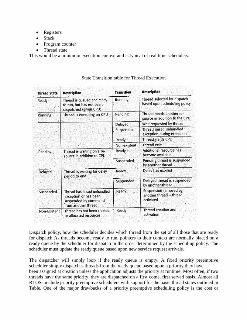
Registers

Stack

Program counter

Thread state

This would be a minimum execution context and is typical of real time schedulers.

State Transition table for Thread Execution

Dispatch policy, how the scheduler decides which thread from the set of all those that are ready

for dispatch As threads become ready to run, pointers to their context are normally placed on a

ready queue by the scheduler for dispatch in the order determined by the scheduling policy. The

scheduler must update the ready queue based upon new service request arrivals.

The dispatcher will simply loop if the ready queue is empty. A fixed priority preemptive

scheduler simply dispatches threads from the ready queue based upon a priority they have

been assigned at creation unless the application adjusts the priority at runtime. Most often, if two

threads have the same priority, they are dispatched on a first come, first served basis. Almost all

RTOSs include priority preemptive schedulers with support for the basic thread states outlined in

Table. One of the major drawbacks of a priority preemptive scheduling policy is the cost or

overhead of the context switch that occurs on every interrupt. a time-slice preemption scheme

where an OS timer tick is generated every so many milliseconds by a programmable interval

timer, have high overhead.

Context Switch

A context switch is the mechanism to store and restore the state or context of a CPU in Process

Control block so that a process execution can be resumed from the same point at a later time.

Using this technique a context switcher enables multiple processes to share a single CPU.

Context switching is an essential part of a multitasking operating system features.

When the scheduler switches the CPU from executing one process to execute another, the

context switcher saves the content of all processor registers for the process being removed from

the CPU, in its process descriptor. The context of a process is represented in the process control

block of a process.

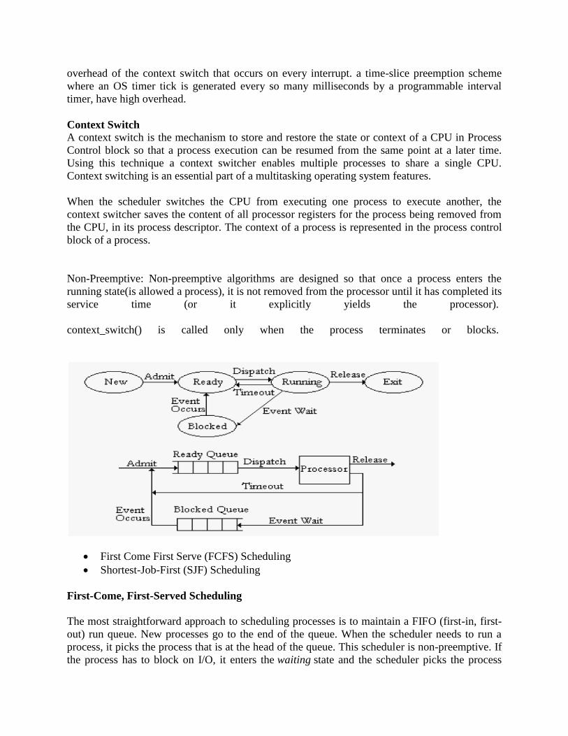
Non-Preemptive: Non-preemptive algorithms are designed so that once a process enters the

running state(is allowed a process), it is not removed from the processor until it has completed its

service time (or it explicitly yields the processor).

context_switch() is called only when the process terminates or blocks.

First Come First Serve (FCFS) Scheduling

Shortest-Job-First (SJF) Scheduling

First-Come, First-Served Scheduling

The most straightforward approach to scheduling processes is to maintain a FIFO (first-in, first-

out) run queue. New processes go to the end of the queue. When the scheduler needs to run a

process, it picks the process that is at the head of the queue. This scheduler is non-preemptive. If

the process has to block on I/O, it enters the waiting state and the scheduler picks the process

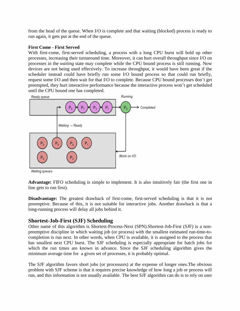
from the head of the queue. When I/O is complete and that waiting (blocked) process is ready to

run again, it gets put at the end of the queue.

First Come - First Served

With first-come, first-served scheduling, a process with a long CPU burst will hold up other

processes, increasing their turnaround time. Moreover, it can hurt overall throughput since I/O on

processes in the waiting state may complete while the CPU bound process is still running. Now

devices are not being used effectively. To increase throughput, it would have been great if the

scheduler instead could have briefly run some I/O bound process so that could run briefly,

request some I/O and then wait for that I/O to complete. Because CPU bound processes don’t get

preempted, they hurt interactive performance because the interactive process won’t get scheduled

until the CPU bound one has completed.

Advantage: FIFO scheduling is simple to implement. It is also intuitively fair (the first one in

line gets to run first).

Disadvantage: The greatest drawback of first-come, first-served scheduling is that it is not

preemptive. Because of this, it is not suitable for interactive jobs. Another drawback is that a

long-running process will delay all jobs behind it.

Shortest-Job-First (SJF) Scheduling Other name of this algorithm is Shortest-Process-Next (SPN).Shortest-Job-First (SJF) is a non-

preemptive discipline in which waiting job (or process) with the smallest estimated run-time-to-

completion is run next. In other words, when CPU is available, it is assigned to the process that

has smallest next CPU burst. The SJF scheduling is especially appropriate for batch jobs for

which the run times are known in advance. Since the SJF scheduling algorithm gives the

minimum average time for a given set of processes, it is probably optimal.

The SJF algorithm favors short jobs (or processors) at the expense of longer ones.The obvious

problem with SJF scheme is that it requires precise knowledge of how long a job or process will

run, and this information is not usually available. The best SJF algorithm can do is to rely on user

estimates of run times. In the production environment where the same jobs run regularly, it may

be possible to provide reasonable estimate of run time, based on the past performance of the

process. But in the development environment users rarely know how their program will execute.

Preemptive : The term preemptive multitasking is used to distinguish a multitasking operating

system, which permits preemption of tasks, from a cooperative multitasking system wherein

processes or tasks must be programmed to yield when they do not need system resources. In

simple terms: Preemptive multitasking involves the use of an interrupt mechanism which

suspends the currently executing process and invokes a scheduler to determine which process

should execute next. Therefore all processes will get some amount of CPU time at any given

time.

In preemptive multitasking, the operating system kernel can also initiate a context switch to

satisfy the scheduling policy's priority constraint, thus preempting the active task. In general,

preemption means "prior seizure of". When the high priority task at that instance seizes the

currently running task, it is known as preemptive scheduling.

The term "preemptive multitasking" is sometimes mistakenly used when the intended meaning is

more specific, referring instead to the class of scheduling policies known as time-shared

scheduling, or time-sharing.

Preemptive multitasking allows the computer system to more reliably guarantee each process a

regular "slice" of operating time. It also allows the system to rapidly deal with important external

events like incoming data, which might require the immediate attention of one or another

process.

Rate-monotonic scheduling (RMS) is a scheduling algorithm used in real-time operating

systems (RTOS) with a static-priority scheduling class. The static priorities are assigned on the

basis of the cycle duration of the job: the shorter the cycle duration is, the higher is the job's

priority.

Deadline-monotonic priority assignment is a priority assignment policy used with fixed priority

pre-emptive scheduling. With deadline-monotonic priority assignment, tasks are assigned

priorities according to their deadlines; the task with the shortest deadline being assigned the

highest priority.

This priority assignment policy is optimal for a set of periodic or sporadic tasks which comply

with the following restrictive system model:

All tasks have deadlines less than or equal to their minimum inter-arrival times (or

periods).

All tasks have worst-case execution times (WCET) that are less than or equal to their

deadlines.

All tasks are independent and so do not block each other's execution (for example by

accessing mutually exclusive shared resources).

No task voluntarily suspends itself.

There is some point in time, referred to as a critical instant, where all of the tasks become

ready to execute simultaneously.

Scheduling overheads (switching from one task to another) are zero.

All tasks have zero release jitter (the time from the task arriving to it becoming ready to

execute).

Earliest deadline first (EDF) or least time to go is a dynamic scheduling algorithm used in real-

time operating systems to place processes in a priority queue. Whenever a scheduling event

occurs (task finishes, new task released, etc.) the queue will be searched for the process closest to

its deadline. This process is the next to be scheduled for execution.

EDF is an optimal scheduling algorithm on preemptive uniprocessors, in the following sense: if a

collection of independent jobs, each characterized by an arrival time, an execution requirement

and a deadline, can be scheduled (by any algorithm) in a way that ensures all the jobs complete

by their deadline, the EDF will schedule this collection of jobs so they all complete by their

deadline.

Least slack time (LST) scheduling is a scheduling algorithm. It assigns priority based on

the slack time of a process. Slack time is the amount of time left after a job if the job was started

now. This algorithm is also known as least laxity first. Its most common use is in embedded

systems, especially those with multiple processors. It imposes the simple constraint that each

process on each available processor possesses the same run time, and that individual processes

do not have an affinity to a certain processor. This is what lends it a suitability to embedded

systems.

This scheduling algorithm first selects those processes that have the smallest "slack time". Slack

time is defined as the temporal difference between the deadline, the ready time and the run time.

This scheduling algorithm first selects those processes that have the smallest "slack time". Slack

time is defined as the temporal difference between the deadline, the ready time and the run time.

More formally, the slack time for a process is defined as:

where is the process deadline, is the real time since the cycle start, and is the remaining

computation time.

Fixed-priority preemptive scheduling Fixed-priority preemptive scheduling is a scheduling system commonly used in real-time

systems. With fixed priority preemptive scheduling, the scheduler ensures that at any given time,

the processor executes the highest priority task of all those tasks that are currently ready to

execute.

The preemptive scheduler has a clock interrupt task that can provide the scheduler with options

to switch after the task has had a given period to execute the time slice. This scheduling system

has the advantage of making sure no task hogs the processor for any time longer than the time

slice. However, this scheduling scheme is vulnerable to process or thread lockout: since priority

is given to higher-priority tasks, the lower-priority tasks could wait an indefinite amount of time.

One common method of arbitrating this situation is aging, which gradually increments the

priority of waiting processes and threads, ensuring that they will all eventually execute.

The scheduling problem must be further constrained to derive a formal mathematical model that

proves deterministic behavior. Clearly it is impossible to prove deterministic behavior for a

system that has nondeterministic inputs. Liu and Layland recognized this and proposed what they

believed to be a reasonable set of assumptions and constraints on real systems to formulate a

deterministic model. The assumptions and constraints are

A1: All services requested on periodic basis, the period is constant

A2: Completion time < period

A3: Service requests are independent (no known phasing)

A4: Runtime is known and deterministic (WCET may be used)

C1: Deadline = period by definition

C2: Fixed priority preemptive, run- to- completion scheduling .

A5: Critical instant—longest response time for a service occurs when all system services are

requested simultaneously (maximum interference case for lowest priority service).

Layland in their paper.

Given the fixed priority preemptive scheduling framework and assumptions described in the

preceding list, we can now examine alternatives for assigning priorities and identify a policy that

is optimal. Showing that the RM policy is optimal is most easily accomplished by inspecting a

system with a small number of services. An example with two services follows. Given services

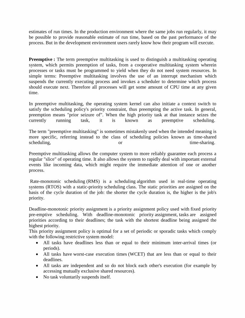
S1and S2 with periods T1 and T2, execution times C1 and C2) and release periods T2 > T1, take,

for example, T1=2, T2= 5, C1=1, C2 = 2, and then if prio(S1) > prio(S2), note Figure S1 Makes

Deadline if prio(S1) > prio(S2).

In this two service example, the only other policy (swapping priorities from the preceding

example) does not work. Given services S1 and S2 with periods T1 and T2 and C1 and C2with

T2 > T1, for example, T1 =2, T2 = 5, C, = 1, C2 = 2, and then if prio(S2) > prio(S1).

The conclusion that can be drawn is that for a two service system, the RM policy is optimal,

whereas the only alternative is not optimal because the alternative policy fails when a workable

schedule does exist! The same argument can be posed for a three-service system, a four service

system, and finally an N service system. In all cases, it can be shown that the RM policy is

optimal.

Real-time operating systems

Many real time embedded systems include an RTOS , which provides CPU scheduling, memory

management, and driver interfaces for 1/0 in addition to boot or BSP (Board Support Package)

firmware.

Key features that an RTOS or an embedded realtime Linux distribution should have include the

following:

A fully preemptable kernel so that an interrupt or realtime task can preempt the kernel

scheduler and kernel services with priority.

Low well bounded interrupt latency.

Low well bounded process, task, or thread context switch latency

Capability to fully control all hardware resources and to override any built in operating

system resource management

E Execution tracing tools

Cross compiling, cross debugging, and host-to-target interface tools to support

code development on an embedded microprocessor.

Full support for POSIX 1003.1b synchronous and asynchronous inter task

communication, control, and scheduling.

Priority inversion safe options for mutual exclusion semaphores (the mutual exclusion

semaphore referred to in this text includes features that extend the early concepts for

semaphores introduced by Dijkstra)

Capability to lock memory address ranges into cache

Capability to lock memory address ranges into working memory if virtual memory with

paging is implemented.

High precision time stamping, interval timers, and real time clocks and virtual timers

The VxWorks, ThreadX, Nucleus, Micro-C-OS, RTEMS and many other available realtime

operating systems provide the features in the preceding list.

In general, an RTOS provides a threading mechanism, in some cases referred to as a task

context, which is the implementation of a service. A service is the theoretical concept of an

execution context. The RTOS most often implements this as a thread of execution, with a well

known entry point into a code (text) segment, through a function, and a memory context for this

thread of execution, which is called the thread context. Typical RTOS CPU scheduling is fixed

priority preemptive, with the capability to modify priorities at runtime by applications, therefore

also supporting dynamic priority preemptive. Real time response with bounded latency for any

number of services requires preemption based upon interrupts. Systems where latency bounds

are more relaxed might instead use polling for events and run threads to completion, increasing

efficiency by avoiding disruptive asynchronous interrupt context switches.

An RTOS provides priority preemptive scheduling as a mechanism that allows an application to

implement a variety of scheduling policies:

RM (Rate Monotonic) or DM (Deadline Monotonic), fixed priority

EDF (Earliest Deadline First) or LLF (Least Laxity First), dynamic priority

Simple run to completion cooperative tasking

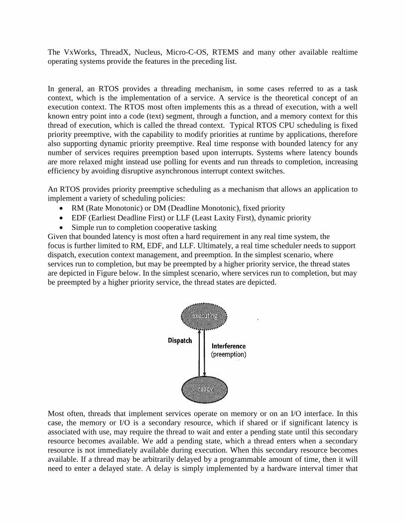
Given that bounded latency is most often a hard requirement in any real time system, the

focus is further limited to RM, EDF, and LLF. Ultimately, a real time scheduler needs to support

dispatch, execution context management, and preemption. In the simplest scenario, where

services run to completion, but may be preempted by a higher priority service, the thread states

are depicted in Figure below. In the simplest scenario, where services run to completion, but may

be preempted by a higher priority service, the thread states are depicted.

Most often, threads that implement services operate on memory or on an I/O interface. In this

case, the memory or I/O is a secondary resource, which if shared or if significant latency is

associated with use, may require the thread to wait and enter a pending state until this secondary

resource becomes available. We add a pending state, which a thread enters when a secondary

resource is not immediately available during execution. When this secondary resource becomes

available. If a thread may be arbitrarily delayed by a programmable amount of time, then it will

need to enter a delayed state. A delay is simply implemented by a hardware interval timer that

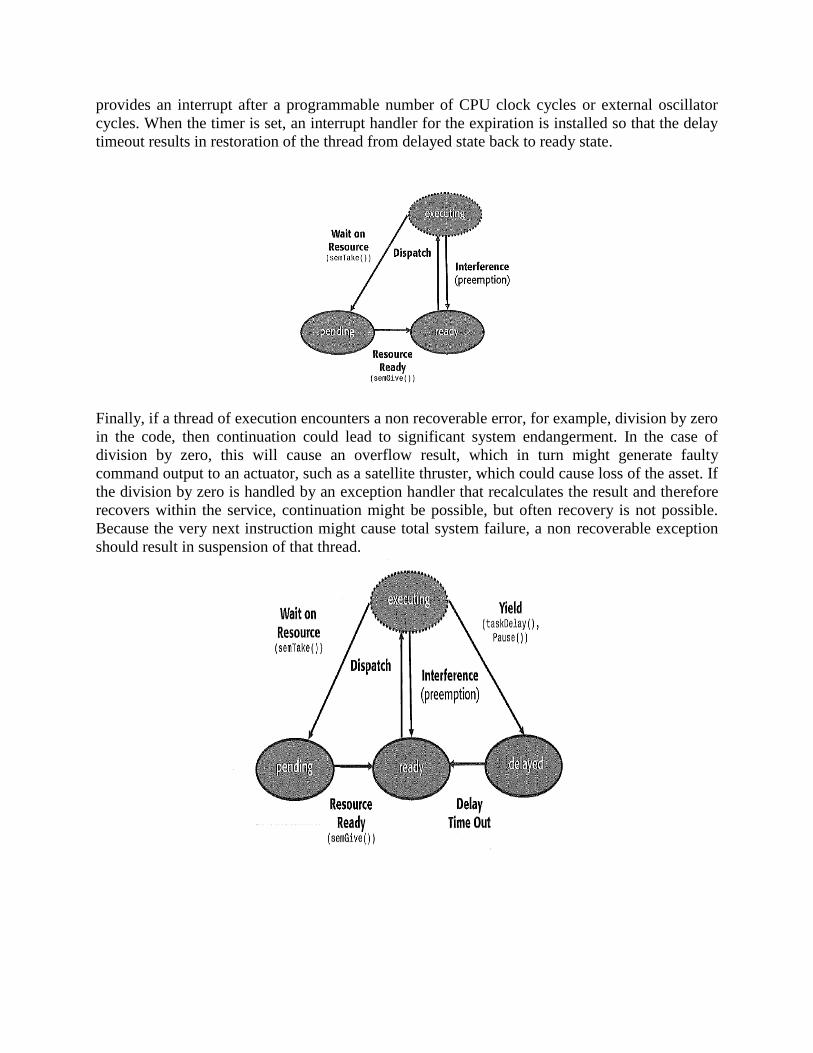
provides an interrupt after a programmable number of CPU clock cycles or external oscillator

cycles. When the timer is set, an interrupt handler for the expiration is installed so that the delay

timeout results in restoration of the thread from delayed state back to ready state.

Finally, if a thread of execution encounters a non recoverable error, for example, division by zero

in the code, then continuation could lead to significant system endangerment. In the case of

division by zero, this will cause an overflow result, which in turn might generate faulty

command output to an actuator, such as a satellite thruster, which could cause loss of the asset. If

the division by zero is handled by an exception handler that recalculates the result and therefore

recovers within the service, continuation might be possible, but often recovery is not possible.

Because the very next instruction might cause total system failure, a non recoverable exception

should result in suspension of that thread.

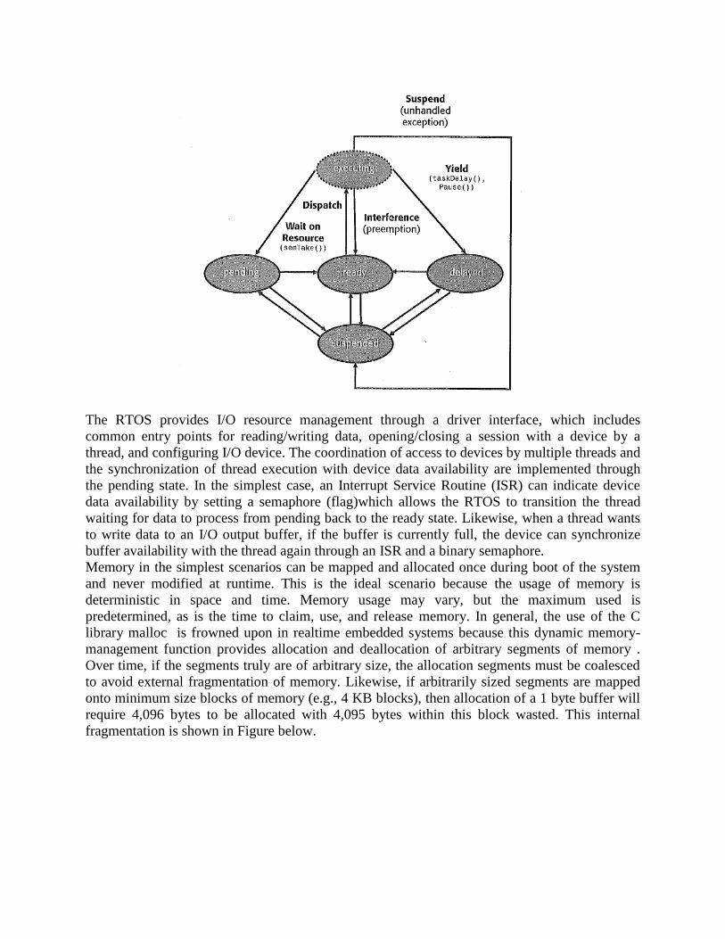
The RTOS provides I/O resource management through a driver interface, which includes

common entry points for reading/writing data, opening/closing a session with a device by a

thread, and configuring I/O device. The coordination of access to devices by multiple threads and

the synchronization of thread execution with device data availability are implemented through

the pending state. In the simplest case, an Interrupt Service Routine (ISR) can indicate device

data availability by setting a semaphore (flag)which allows the RTOS to transition the thread

waiting for data to process from pending back to the ready state. Likewise, when a thread wants

to write data to an I/O output buffer, if the buffer is currently full, the device can synchronize

buffer availability with the thread again through an ISR and a binary semaphore.

Memory in the simplest scenarios can be mapped and allocated once during boot of the system

and never modified at runtime. This is the ideal scenario because the usage of memory is

deterministic in space and time. Memory usage may vary, but the maximum used is

predetermined, as is the time to claim, use, and release memory. In general, the use of the C

library malloc is frowned upon in realtime embedded systems because this dynamic memory-

management function provides allocation and deallocation of arbitrary segments of memory .

Over time, if the segments truly are of arbitrary size, the allocation segments must be coalesced

to avoid external fragmentation of memory. Likewise, if arbitrarily sized segments are mapped

onto minimum size blocks of memory (e.g., 4 KB blocks), then allocation of a 1 byte buffer will

require 4,096 bytes to be allocated with 4,095 bytes within this block wasted. This internal

fragmentation is shown in Figure below.

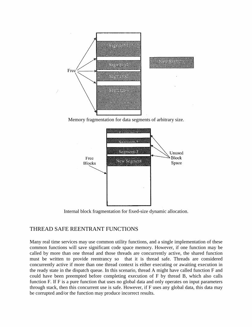
Memory fragmentation for data segments of arbitrary size.

Internal block fragmentation for fixed-size dynamic allocation.

THREAD SAFE REENTRANT FUNCTIONS

Many real time services may use common utility functions, and a single implementation of these

common functions will save significant code space memory. However, if one function may be

called by more than one thread and those threads are concurrently active, the shared function

must be written to provide reentrancy so that it is thread safe. Threads are considered

concurrently active if more than one thread context is either executing or awaiting execution in

the ready state in the dispatch queue. In this scenario, thread A might have called function F and

could have been preempted before completing execution of F by thread B, which also calls

function F. If F is a pure function that uses no global data and only operates on input parameters

through stack, then this concurrent use is safe. However, if F uses any global data, this data may

be corrupted and/or the function may produce incorrect results.

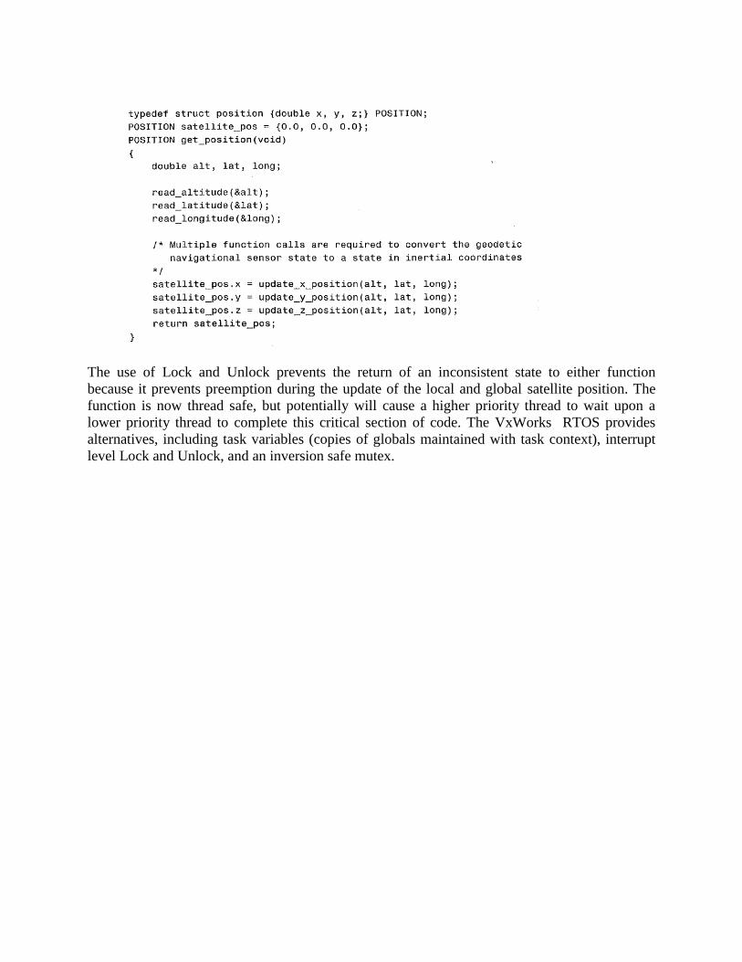
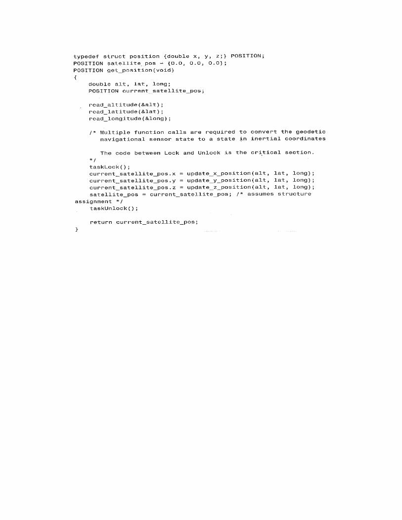
The use of Lock and Unlock prevents the return of an inconsistent state to either function

because it prevents preemption during the update of the local and global satellite position. The

function is now thread safe, but potentially will cause a higher priority thread to wait upon a

lower priority thread to complete this critical section of code. The VxWorks RTOS provides

alternatives, including task variables (copies of globals maintained with task context), interrupt

level Lock and Unlock, and an inversion safe mutex.

Processing Introduction

Preemptive Fixed-Priority Policy

Feasibility

Rate Monotonic Least Upper Bound (RM LUB)

Necessary and Sufficient (N&S) Feasibility

Deadline-Monotonic (DM) Policy

Dynamic Priority Policies

INTRODUCTION

Processing input data and producing output data for a system response in real time does not

necessarily require large CPU resources, but rather careful use of CPU resources. Before

considering how to make optimal use of CPU resources in a real-time embedded system, you

must first better understand what is meant by processing in real time. The mantra of realtime

system correctness is that the system must not only produce the required output response for a

given input (functional correctness), but that it must do so in a timely manner (before a deadline).

A deadline in a real-time system is a relative time after a service request by which time the

system must produce a response. The relative deadline seems to be a simple concept, but a more

formal specification of real-time services is helpful due to the many types of applications. For

example, the processing in a Voice or video.

Real- time system is considered high quality if the service continuously provides output neither

too early nor too late, without too much latency and without too much jitter between frames.

Similarly, in digital control applications, the ideal system has a constant time delay between

sensor sampling and actuator outputs

PREEMPTIVE FIXED-PRIORITY POLICY

Given that the RM priority assignment policy is optimal, we now want to determine whether a

proposed set of services is feasible. Feasible means that the proposed set of services can be

scheduled given a fixed and known amount of CPU resource. One such test is the RM LUB: Liu

and Layland proposed this simple feasibility test they call the RM Least Upper Bound (RM

LUB). The RM LUB is defined as

U: Utility of the CPU resource achievable

C: Execution time of Service i

m: Total number of services in the system sharing common CPU resources

T : Release period of Service i

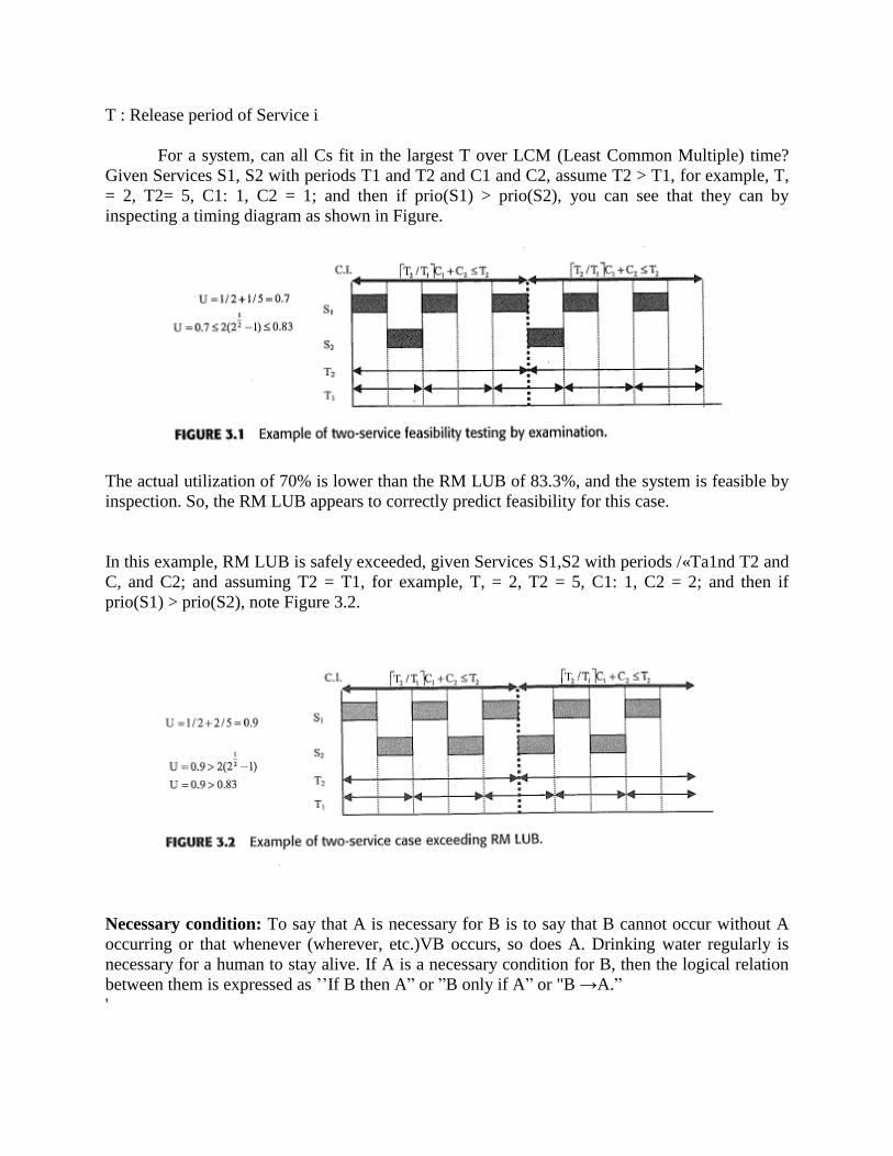
For a system, can all Cs fit in the largest T over LCM (Least Common Multiple) time?

Given Services S1, S2 with periods T1 and T2 and C1 and C2, assume T2 > T1, for example, T,

= 2, T2= 5, C1: 1, C2 = 1; and then if prio(S1) > prio(S2), you can see that they can by

inspecting a timing diagram as shown in Figure.

The actual utilization of 70% is lower than the RM LUB of 83.3%, and the system is feasible by

inspection. So, the RM LUB appears to correctly predict feasibility for this case.

In this example, RM LUB is safely exceeded, given Services S1,S2 with periods /«Ta1nd T2 and

C, and C2; and assuming T2 = T1, for example, T, = 2, T2 = 5, C1: 1, C2 = 2; and then if

prio(S1) > prio(S2), note Figure 3.2.

Necessary condition: To say that A is necessary for B is to say that B cannot occur without A

occurring or that whenever (wherever, etc.)VB occurs, so does A. Drinking water regularly is

necessary for a human to stay alive. If A is a necessary condition for B, then the logical relation

between them is expressed as ’’If B then A” or ”B only if A” or "B →A.”

'

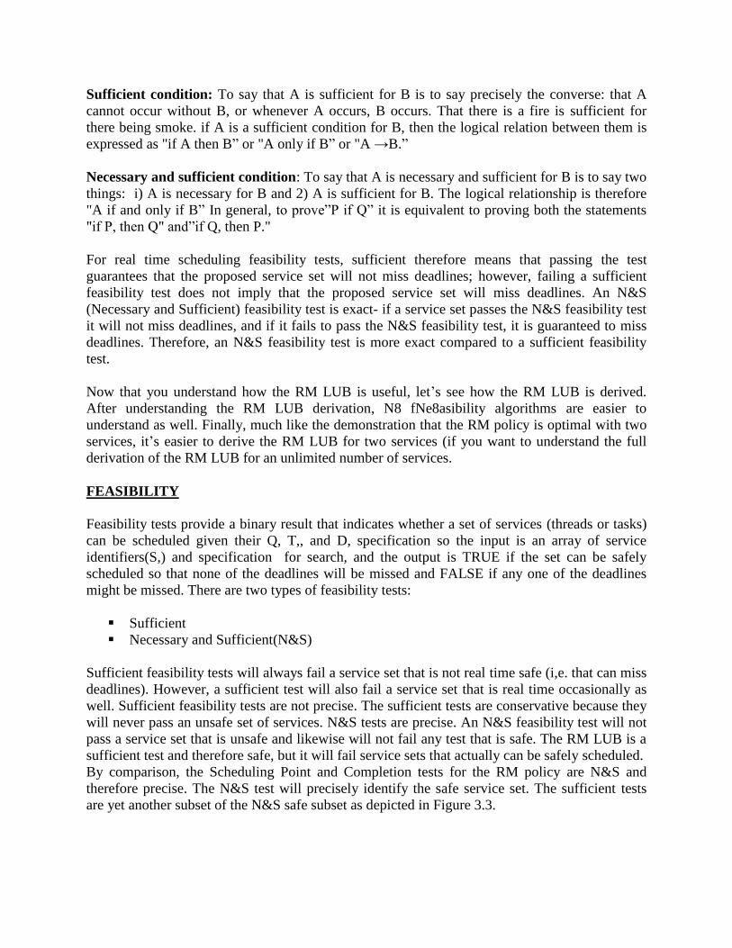
Sufficient condition: To say that A is sufficient for B is to say precisely the converse: that A

cannot occur without B, or whenever A occurs, B occurs. That there is a fire is sufficient for

there being smoke. if A is a sufficient condition for B, then the logical relation between them is

expressed as "if A then B” or "A only if B” or "A →B.”

Necessary and sufficient condition: To say that A is necessary and sufficient for B is to say two

things: i) A is necessary for B and 2) A is sufficient for B. The logical relationship is therefore

"A if and only if B” In general, to prove”P if Q” it is equivalent to proving both the statements

"if P, then Q" and”if Q, then P."

For real time scheduling feasibility tests, sufficient therefore means that passing the test

guarantees that the proposed service set will not miss deadlines; however, failing a sufficient

feasibility test does not imply that the proposed service set will miss deadlines. An N&S

(Necessary and Sufficient) feasibility test is exact- if a service set passes the N&S feasibility test

it will not miss deadlines, and if it fails to pass the N&S feasibility test, it is guaranteed to miss

deadlines. Therefore, an N&S feasibility test is more exact compared to a sufficient feasibility

test.

Now that you understand how the RM LUB is useful, let’s see how the RM LUB is derived.

After understanding the RM LUB derivation, N8 fNe8asibility algorithms are easier to

understand as well. Finally, much like the demonstration that the RM policy is optimal with two

services, it’s easier to derive the RM LUB for two services (if you want to understand the full

derivation of the RM LUB for an unlimited number of services.

FEASIBILITY

Feasibility tests provide a binary result that indicates whether a set of services (threads or tasks)

can be scheduled given their Q, T,, and D, specification so the input is an array of service

identifiers(S,) and specification for search, and the output is TRUE if the set can be safely

scheduled so that none of the deadlines will be missed and FALSE if any one of the deadlines

might be missed. There are two types of feasibility tests:

Sufficient

Necessary and Sufficient(N&S)

Sufficient feasibility tests will always fail a service set that is not real time safe (i,e. that can miss

deadlines). However, a sufficient test will also fail a service set that is real time occasionally as

well. Sufficient feasibility tests are not precise. The sufficient tests are conservative because they

will never pass an unsafe set of services. N&S tests are precise. An N&S feasibility test will not

pass a service set that is unsafe and likewise will not fail any test that is safe. The RM LUB is a

sufficient test and therefore safe, but it will fail service sets that actually can be safely scheduled.

By comparison, the Scheduling Point and Completion tests for the RM policy are N&S and

therefore precise. The N&S test will precisely identify the safe service set. The sufficient tests

are yet another subset of the N&S safe subset as depicted in Figure 3.3.

RATE MONOTONIC LEAST UPPER BOUND (RM LUB)

Taking the same two service example shown earlier in Figure 3.2, we have the following set of

proposed services. Given Services S1,S2with periods T1 and T2 and execution times C2 and C2,

assume that the services are released with T1 = 2, T2= 5, execute deterministically with C2 = 1,

C2 = 2, and are scheduled by the RM policy so that prio(S2) > prio(S2). If this proposed system

can be shown to be feasible so that it can be scheduled with the RM policy over the LCM (least

common multiple) period derived from all proposed service periods, then the Lehoczky, Shah,

and Ding theorem guarantees it real time safe. The theorem is based upon the fact that given the

periodic releases of each service, the LCM schedule will simply repeat over and over as shown

in Figure 3.4.

Note that there can be up to releases of S1 during T2 as indicated by the

#1, #2, and #3 execution traces for S1in Figure 3.4. Furthermore, note that in this particular

scenario, the utilization U is 90%.” The CI (Critical Instant) is a worst case assumption that the

demands upon the system might include simultaneous requests for service by all services in the

system! This eliminates the complexity of assuming some sort of known relationship or phasing

between service requests and makes the RM LUB a more general result.

Given this motivating two service example, we can now devise a strategy to derive the RM LUB

for any given set of services S for which each service 81has an arbitrary Ci,Ti. Taking this

example, we examine two cases:

Case 1: C1 short enough to fit all three releases in T2 (fitsS2critical time zone)

Case 2: C1 too large to fit last release in T2 (doesn’t fit S2critical time zone)

Examine U in both cases to find common U upper bound. The critical time zone is depicted in

Figure 3.5.

The S2 critical time zone is best understood by considering the condition where S1 releases

occur the maximum number of times and for a duration that uses all possible time during

T2without actually causing S2to miss its deadline. So, Case 1 where S1total resource required

just fits the S2critical time zone (T2-C2) is shown in Figure 3.5.

In Case 1, all three S1releases requiring C1 execution time fit in T2 as shown in Figure 3.5. This

is expressed by

C2>T2—C1[T2/T1] (3.2)

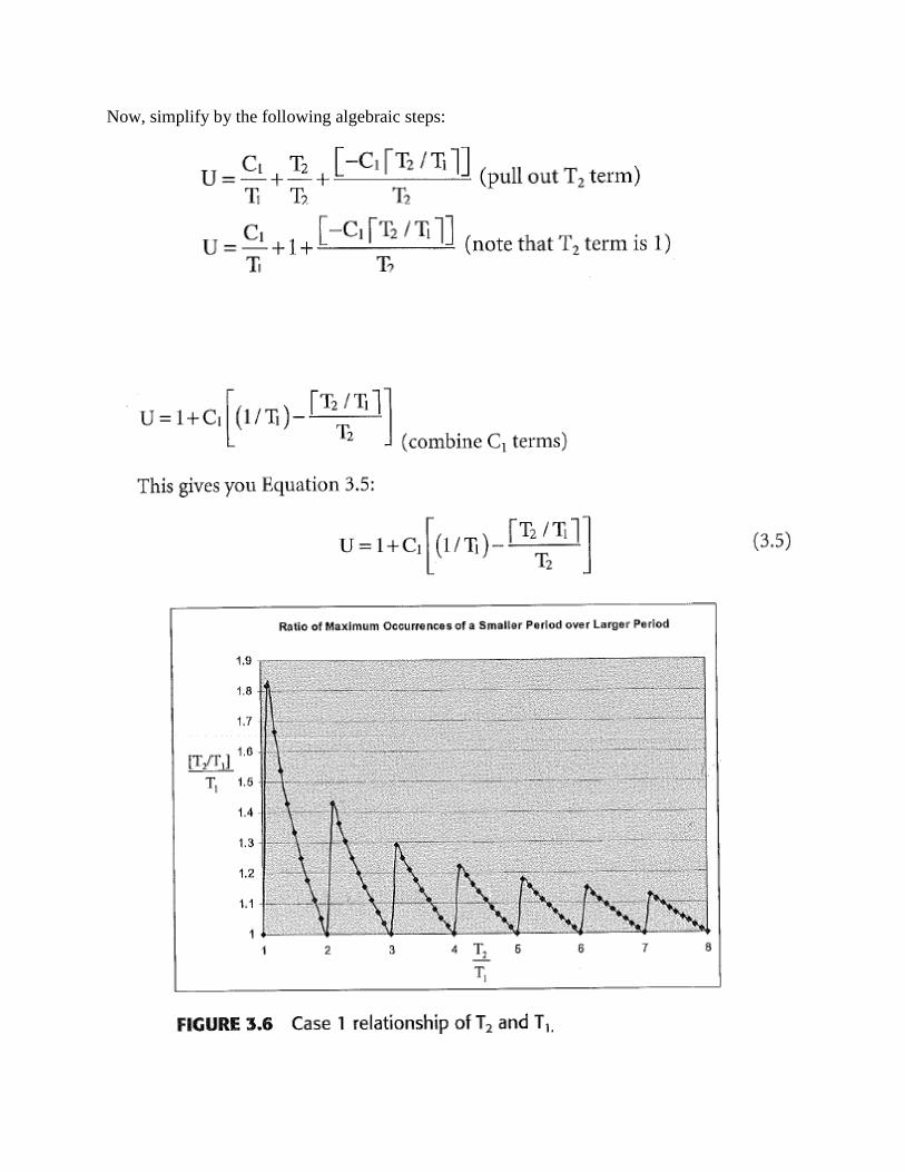
Now, simplify by the following algebraic steps:

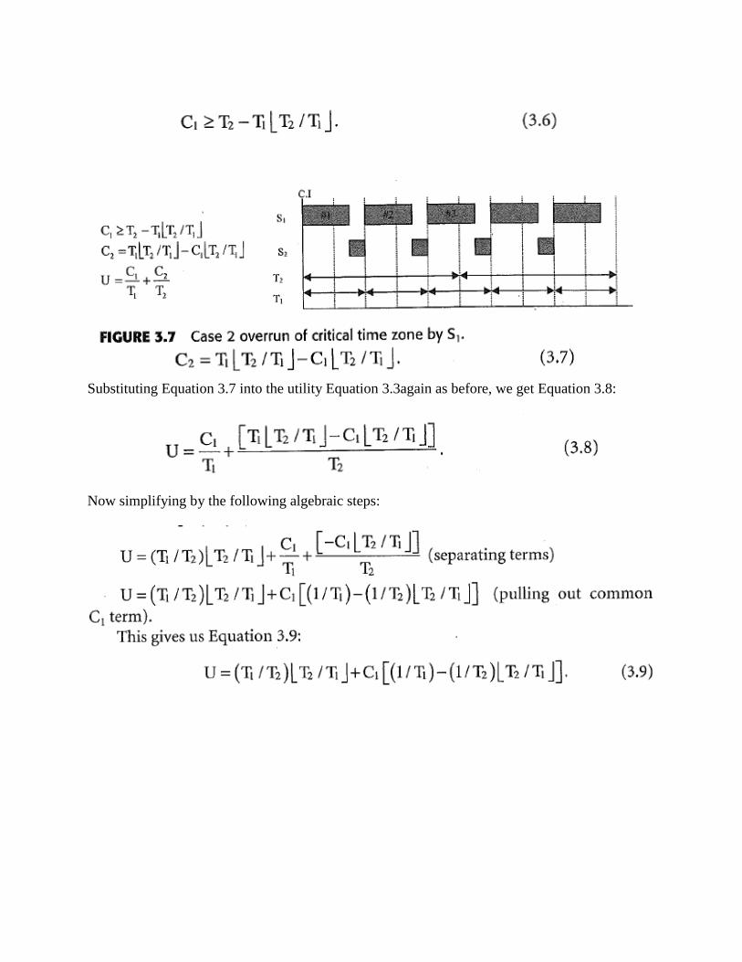
Substituting Equation 3.7 into the utility Equation 3.3again as before, we get Equation 3.8:

Now simplifying by the following algebraic steps:

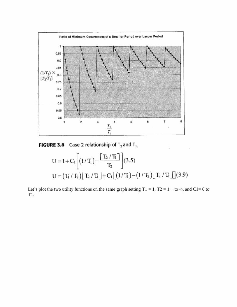
Let’s plot the two utility functions on the same graph setting T1 = 1, T2 = 1 + to ∞, and C1= 0 to

T1.

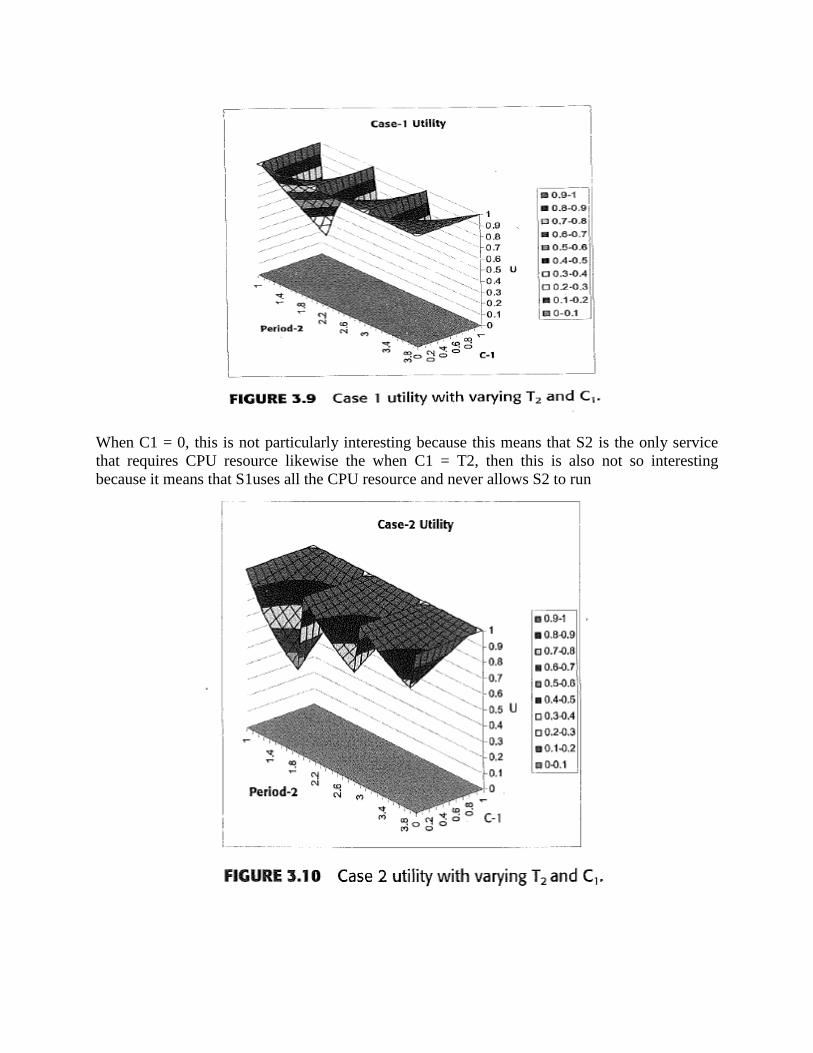
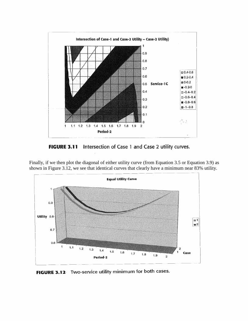
When C1 = 0, this is not particularly interesting because this means that S2 is the only service

that requires CPU resource likewise the when C1 = T2, then this is also not so interesting

because it means that S1uses all the CPU resource and never allows S2 to run

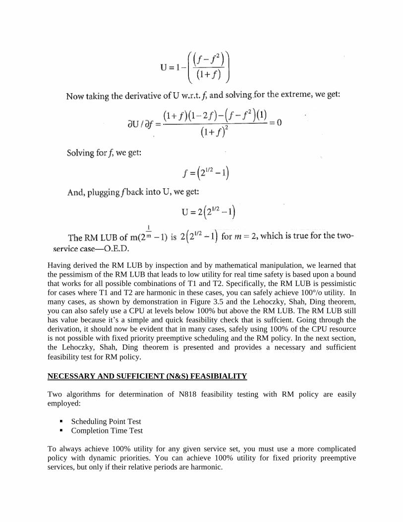
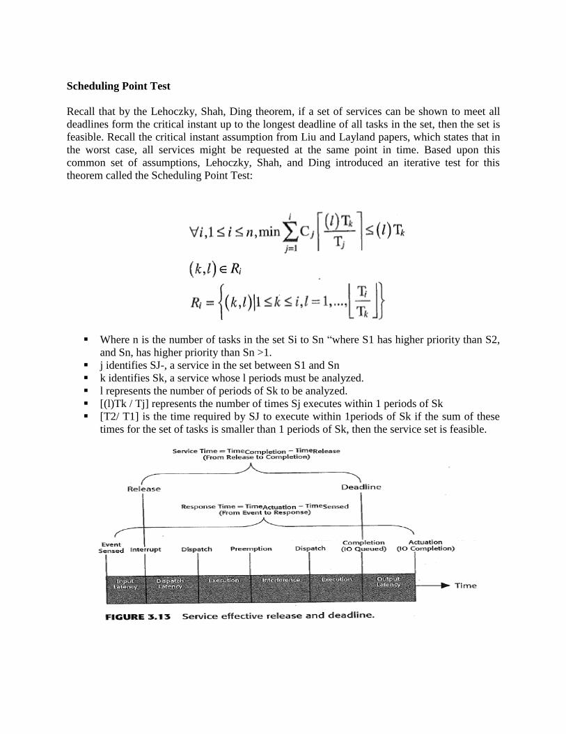
Finally, if we then plot the diagonal of either utility curve (from Equation 3.5 or Equation 3.9) as

shown in Figure 3.12, we see that identical curves that clearly have a minimum near 83% utility.

Recall that Liu and Layland claim the least upper bound for safe utility given any arbitrary set of

services (any relation between periods and any relation between critical time zones) is defined

as: For two services, .

We have now empirically determined that there is a minimum safe bound on utility for any given

set of services, but in doing so, we can also clearly see that this bound can be exceeded safely for

specifiTc1, T2, and C1 relations.

For completeness, let’s now finish the two service RM LUB proof mathematically. We’ll argue

that the two cases are valid only when they intersect, and given the two sets of equations this can

only occur when C1 is equal for both cases:

Now, plug C1 and C2 simultaneously into the utility equation to get Equation 3.10:

Now, let whole integer number of interferences of S, to S2 over T2 be I= [T2 / T1] and the

fractional interference be f = (T2/ T1) – [T2/ T1]. From this, we can derive a simple expression

for utility:

Equation 3.11 is based upon substitution of I and f into Equation 3.10‘as follows:

By adding and subtracting the same denominator term to Equation 3.11, we can get:

The smallest I possible is 1, and the LUB for U occurs when I is minimized, so we substitute 1

for I to get:

Having derived the RM LUB by inspection and by mathematical manipulation, we learned that

the pessimism of the RM LUB that leads to low utility for real time safety is based upon a bound

that works for all possible combinations of T1 and T2. Specifically, the RM LUB is pessimistic

for cases where T1 and T2 are harmonic in these cases, you can safely achieve 100°/o utility. In

many cases, as shown by demonstration in Figure 3.5 and the Lehoczky, Shah, Ding theorem,

you can also safely use a CPU at levels below 100% but above the RM LUB. The RM LUB still

has value because it’s a simple and quick feasibility check that is suffcient. Going through the

derivation, it should now be evident that in many cases, safely using 100% of the CPU resource

is not possible with fixed priority preemptive scheduling and the RM policy. In the next section,

the Lehoczky, Shah, Ding theorem is presented and provides a necessary and sufficient

feasibility test for RM policy.

NECESSARY AND SUFFICIENT (N&S) FEASIBIALITY

Two algorithms for determination of N818 feasibility testing with RM policy are easily

employed:

Scheduling Point Test

Completion Time Test

To always achieve 100% utility for any given service set, you must use a more complicated

policy with dynamic priorities. You can achieve 100% utility for fixed priority preemptive

services, but only if their relative periods are harmonic.

Scheduling Point Test

Recall that by the Lehoczky, Shah, Ding theorem, if a set of services can be shown to meet all

deadlines form the critical instant up to the longest deadline of all tasks in the set, then the set is

feasible. Recall the critical instant assumption from Liu and Layland papers, which states that in

the worst case, all services might be requested at the same point in time. Based upon this

common set of assumptions, Lehoczky, Shah, and Ding introduced an iterative test for this

theorem called the Scheduling Point Test:

Where n is the number of tasks in the set Si to Sn “where S1 has higher priority than S2,

and Sn, has higher priority than Sn >1.

j identifies SJ-, a service in the set between S1 and Sn

k identifies Sk, a service whose l periods must be analyzed.

l represents the number of periods of Sk to be analyzed.

[(l)Tk / Tj] represents the number of times Sj executes within 1 periods of Sk

[T2/ T1] is the time required by SJ to execute within 1periods of Sk if the sum of these

times for the set of tasks is smaller than 1 periods of Sk, then the service set is feasible.

The C code algorithm is included with test code on the CD-ROM for the Scheduling Point Test.

Note that the algorithm assumes arrays are sorted according to the RM policy where period [0] is

the highest priority and shortest period.

The Completion Time Test is presented as an alternative to the Scheduling Point Test

[Briand99l:

Passing this test requires proving that an(t) is less than or equal to the deadline for Sn which

proves that Sn is feasible. Proving this same property for all S from S1to Sn proves that the

service set is feasible.

DEADLINE-MONOTONIC POLICY

Deadline-monotonic (DM) policy is very similar to RM except that highest priority is assigned to

the service with the shortest deadline. The DM policy is a fixed priority policy. The DM policy

eliminates the original RM assumption that service period must equal service deadline and

allows RM theory to be applied for scenarios even when deadline is less than period. This is

useful for dealing with significant output latency. The DM policy can be shown to be an optimal

fixed priority assignment policy like RM policy because D,-and T,- differ only by a constant

value, and Di ≤ Ti-.The DM policy feasibility tests are most easily implemented as iterative tests

like Scheduling Point and the Completion Time Test for RM policy. The sufficient feasibility

test they first introduced is simple and intuitive:

Ci is the execution time for service i and Ii is the interference time service i experiences over its

deadline Di time period since the time of request for service. Equation 3.12 states that for all

services from 1 to n, if the deadline interval is long enough to contain the service execution time

interval plus all interfering execution time intervals, then the service is feasible. If all services are

feasible, then the system is feasible (real time safe).

Interference to Service S, is due to preemption by all higher priority services S1 to Si-1, and the

total interference time is the number of releases of Sj over the deadline interval Dj The number

of Si interferences is then multiplied by execution time Cj and summed for all Sj. Note that Sj

always has higher priority than Si.

is the worst case number of releases of Sj over the deadline interval for Si. Because the

interference is the worst case number of releases, interference is over accounted for the last

interference may be only partial. So, there will be [Di/Tj] full interferences and some partial

interference from the last additional interference. So, we can better account for the partial

interference with

DYNAMIC PRIORITY POLICIES

Priority preemptive dynamic priority systems can be thought of as a more complex class of

priority preemptive where priorities are adjusted by the scheduler every time a new service is

released and ready to run; Furthermore, it shows that a related dynamic priority policy, LLF

(Least Laxity First), also succeeds where RM fails. Like EDF, LLF is a dynamic priority policy

where services on the ready queue are assigned higher priority if their laxity is the least. Laxity is

the time difference between their deadline and remaining computation time. This requires the

scheduler time, and remaining computation time for all services, and to reassign priorities to all

services on every-preemption. Estimating remaining computation time for each service can be

difficult and typically requires a worst case approximation. Like EDF, LLF can also schedule

100% of the CPU for schedules that can’t be scheduled by the static RM policy.

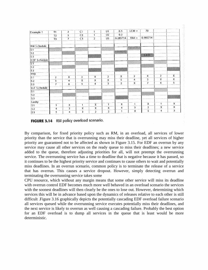
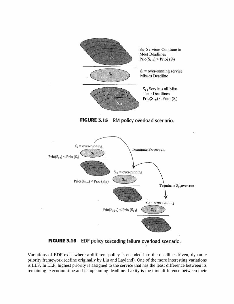
By comparison, for fixed priority policy such as RM, in an overload, all services of lower

priority than the service that is overrunning may miss their deadline, yet all services of higher

priority are guaranteed not to be affected as shown in Figure 3.15. For EDF an overrun by any

service may cause all other services on the ready queue to miss their deadlines; a new service

added to the queue, therefore adjusting priorities for all, will not preempt the overrunning

service. The overrunning service has a time to deadline that is negative because it has passed, so

it continues to be the highest priority service and continues to cause others to wait and potentially

miss deadlines. In an overrun scenario, common policy is to terminate the release of a service

that has overrun. This causes a service dropout. However, simply detecting overrun and

terminating the overrunning service takes some

CPU resource, which without any margin means that some other service will miss its deadline

with overrun control EDF becomes much more well behaved in an overload scenario the services

with the soonest deadlines will then clearly be the ones to lose out. However, determining which

services this will be in advance based upon the dynamics of releases relative to each other is still

difficult .Figure 3.16 graphically depicts the potentially cascading EDF overload failure scenario

all services queued while the overrunning service executes potentially miss their deadlines, and

the next service is likely to overrun as well causing a cascading failure. Probably the best option

for an EDF overload is to dump all services in the queue that is least would be more

deterministic.

Variations of EDF exist where a different policy is encoded into the deadline driven, dynamic

priority framework (define originally by Liu and Layland). One of the more interesting variations

is LLF. In LLF, highest priority is assigned to the service that has the least difference between its

remaining execution time and its upcoming deadline. Laxity is the time difference between their

deadline and remaining computation time for a service. Determining the least laxity service

requires the scheduler to know all outstanding service request times, their deadlines, the current

time, and remaining computation time for all services. After all this is known, the scheduler must

then reassign priorities to all services on every event that adds another service to the ready

queue. Estimating remaining computation time for each service can be difficult and typically

requires a worst case approximation. The LLF policy encodes the concept of imminence, which

intuitively makes sense every student knows that they should work on the homework where they

have the most to do and which is due soonest first unless of course that particular homework is

not worth much credit. In some sense, all priority encoding policies, dynamic or static, miss the

point what we really want to do is encode which service is most important and make sure that it

gets the resources it needs first. We want an intelligent scheduler, like a student who takes into

consideration laxity, impact of missing a deadline for a given assignment, cost of dropping one

or more, and then intelligently determines how to spend resources for maximum benefit.

In fact, since the landmark Liu and Layland formalization of RM and deadline driven

scheduling, most of the processor resource research has been oriented to one of four things:

Generalization and reducing constraints for RM application

Solving problems related to RM application for real systems

Devising alternative policies for deadline—driven scheduling

Devising new soft real time policies to reduce margin required in RM policy

I/O Resources

Introduction

Worst Case Execution Time

Intermediate I/O

Execution Efficiency

I/O Architecture

Most services, unless they are trivial, involve some intermediate I/O after the initial sensor input

and before the final posting of output data to a write buffer. This intermediate I/O is most often

MMR (Memory Mapped Register) or memory device I/ O. If this intermediate I/O has single

core cycle latency, zero wait state then, it has no additional impact on the service response time.

However, if the intermediate I/O stalls the CPU core, then this increases the response time while

the CPU processing pipeline is stalled. Rather than considering this intermediate I/O as device

I/O, it is more easily modelled as execution efficiency. Device I/O latency is hundreds,

thousands, and even millions of core cycles. By comparison, intermediate I/O latency is typically

tens or hundreds of core cycles more latency than this is possible, and then the core hardware

design should be reworked.

WORST-CASE EXECUTION TIME

Ideally the execution time for a service release would be deterministic. For simple

microprocessor architectures, this may be true. The Intel®8088 and the Motorola® 68000, for

example, have no CPU pipeline, no cache, and given memory that has no wait states, you can

take a block of code and count the instructions from start to finish. Furthermore, for these

architectures, the number of CPU cycles required to execute each instruction is known some

instructions may take more cycles than others, but all are known numbers. So, the total number

of CPU clock cycles required to execute a block of code can be calculated. To compute

deterministic execution time for a service, the following system characteristics are necessary:

Exact number of instructions executed from service release input up to response output.

The exact number of CPU clock cycles for each instruction is known.

The number of CPU clock cycles for a given instruction is constant.

The thrust function is often known for a particular type of thrusters. One method to find the root

of any function is to iterate, bisecting an interval to define x and feeding the bisection value into

F(x) = 0 to test how close the current guess for x is to zero. If the guess is higher, then a lesser or

greater sub interval will be selected for the next iteration. If F(x) is a continuous function, then

with successive iterations, the interval will become diminishingly small and the bisection of that

interval, or x, will come closer and closer to the true value of x where F(x) is zero. How much

iteration will this take? The answer depends upon the following requirements:

Accuracy of x needed

Complexity of the function F(x)

The initial interval

Finally, some functions may actually have more than one solution as well. Many numerical

methods are similar to finding roots by bisection in that they require a total path length that

varies with the input. For such algorithms, you need to place an upper bound on the path length

to define WCET (Worst Case Execution Time).

This is typified by the RISC (Reduced Instruction Set Computer) with instruction pipelining and

use of memory caches. As CPU core clock rates increased, memory access latency for

comparably scaled capacity has generally not kept pace. So, most RISC pipelined architectures

make use of cache, a small zero wait state (single CPU cycle access latency) memory.

Unfortunately, cache is too small to hold many applications. So, set associative memories are

used to temporarily hold main memory data when the cache holds data for an address referenced

by a program, this is a hit, and the single cycle access to data and/or code allows the CPU

pipeline to fetch an instruction or load data into a register in a single cycle. A cache miss,

however, stalls the pipeline. Furthermore, 1/0 from MMRs (Memory Mapped Registers) may

require more than a single CPU core cycle and will likewise stall the CPU pipeline if the data is

needed for the next instruction. Detecting potential stalls and avoiding them is an art that can

increase execution efficiency overall for a CPU for example, instructions that cause an MMR

read can be executed out of order so that the instruction requiring the read data is executed as late

as possible, delaying the potential pipeline stall.

The efficiency is therefore data and code driven and not deterministic. So, execution efficiency

will vary, even for the same block of code, because cache contents may not only be a function of

the current thread of execution, but also of the previous threads that executed in the past. In

summary, WCET is a function of the longest path length and the efficiency in executing that

path. Equation 4.1 describes WCET:

The CPI is a figure that describes efficiency in pipelined execution as the number of Clocks Per

Instruction on average that are required to execute each instruction in a block of code. In the next

two sections, “Increasing Efficiency” and “Overlapping Execution with I/O,” .The longest path

instruction count must be determined by inspection, formal software engineering proof, or by

actual instruction count traces in a simulator or with the target CPU architecture. Warning most

CPU core documentation states a CPI that is best case rather than worst case.

For full determinism in WCET for hard real time systems, you must guarantee the following:

All memory access is to known latency memory, including locked cache or main memory

with zero or bounded wait states.

Unlocked cache hits are not expected in unlocked cache because the hit rate is not

deterministic. ,

Overlap of CPU and device I/O is not expected nor required to meet deadlines.

All other pipeline hazards in addition to cache misses and device I/O read/write stalls are

lumped into CPI and taken as worst case (e.g. branch-density * branch penalty).

Longest path is known, and instruction count for it is known.

For soft real time systems, you can allow occasional service drop outs limited overruns and

therefore use ACET (Average Case Execution Time). The ACET can be estimated from the

following information:

Expected L1 and L2 cache hit/miss ratio and cache miss penalty.

Expected overlap of CPU and device I/ O required meeting deadlines.

All other pipeline hazards are typically secondary and can be ignored like branch mis-

prediction.

Average length path is known, and the instruction count for it is known.

In these equations, the effective CPI accounts for secondary pipeline hazards such as branch

mispredictions. The term NOA (Non Overlap Allowed) is 1.0 if 10 time is not overlapped with

processing at all.

INTERMEDIATE I/O

In a non preemptive run to completion system with a pipelined CPU, six key related equations

describe CPU I/O overlaps. Note that the I/O described here is device I/O that occurs during the

service execution, rather than the initial I/O, which releases the service in the first place. In some

sense, the device I/ O occurring during service execution can be considered micro I/O and

usually consists of MMR access rather than block oriented DMA (Direct Memory Access) I/O.

First, you must understand what it means to overlap 1/O with CPU. Consider the following

overlap definitions:

ICT = Instruction Count Time (Time to execute a block of instructions with no stalls =

CPU Cycles * CPU Clock Period)

IOT = Bus Interface I/O Time (Bus I/O Cycles X Bus Clock Period)

OR = Overlap Required percentage cycles that must be concurrent with I/O cycles

NOA = Non Overall Allowable for Si -to meet Di percentage of CPU cycles that can be

in addition to I/O cycle time without missing service deadline

D,-= Deadline for Service Si relative to release (interrupt initiating execution)

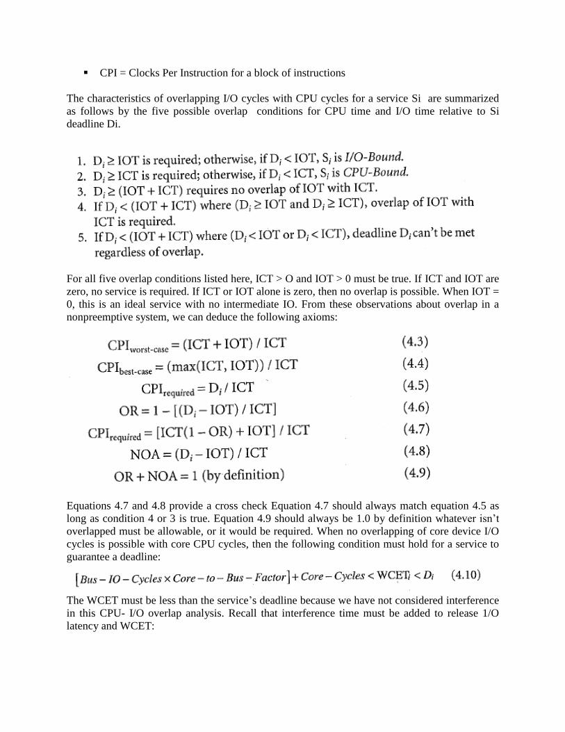
CPI = Clocks Per Instruction for a block of instructions

The characteristics of overlapping I/O cycles with CPU cycles for a service Si are summarized

as follows by the five possible overlap conditions for CPU time and I/O time relative to Si

deadline Di.

For all five overlap conditions listed here, ICT > O and IOT > 0 must be true. If ICT and IOT are

zero, no service is required. If ICT or IOT alone is zero, then no overlap is possible. When IOT =

0, this is an ideal service with no intermediate IO. From these observations about overlap in a

nonpreemptive system, we can deduce the following axioms:

Equations 4.7 and 4.8 provide a cross check Equation 4.7 should always match equation 4.5 as

long as condition 4 or 3 is true. Equation 4.9 should always be 1.0 by definition whatever isn’t

overlapped must be allowable, or it would be required. When no overlapping of core device I/O

cycles is possible with core CPU cycles, then the following condition must hold for a service to

guarantee a deadline:

The WCET must be less than the service’s deadline because we have not considered interference

in this CPU- I/O overlap analysis. Recall that interference time must be added to release 1/O

latency and WCET:

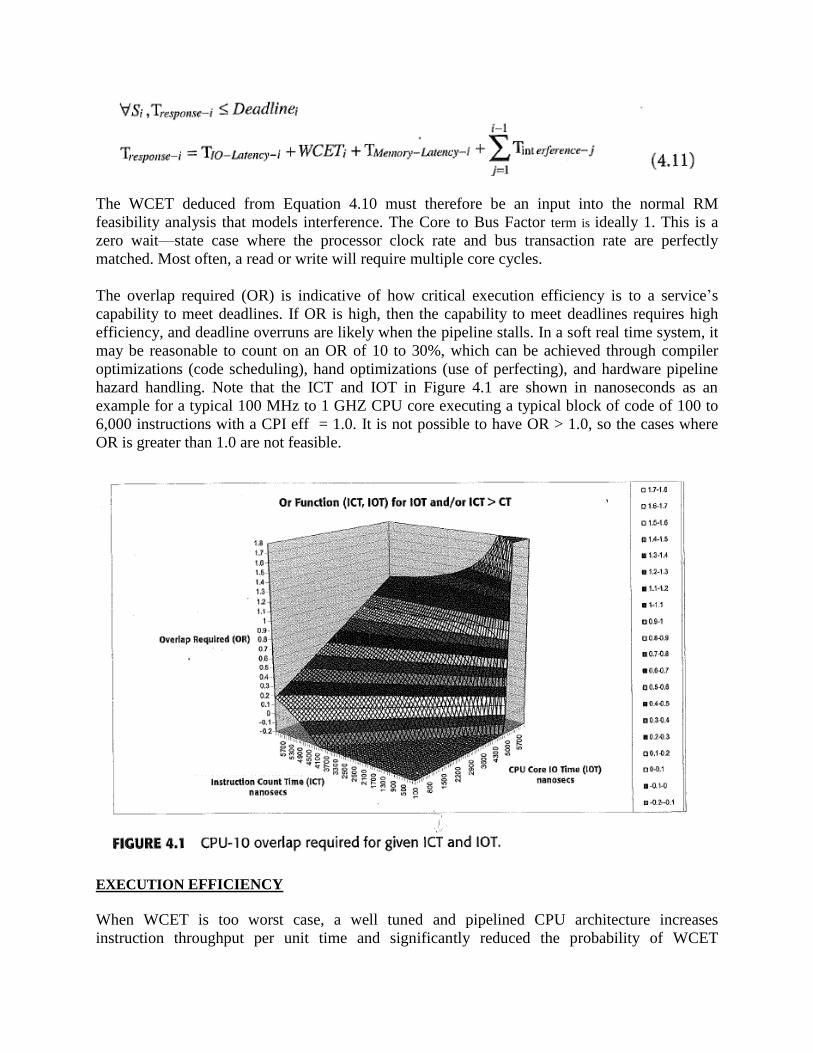
The WCET deduced from Equation 4.10 must therefore be an input into the normal RM

feasibility analysis that models interference. The Core to Bus Factor term is ideally 1. This is a

zero wait—state case where the processor clock rate and bus transaction rate are perfectly

matched. Most often, a read or write will require multiple core cycles.

The overlap required (OR) is indicative of how critical execution efficiency is to a service’s

capability to meet deadlines. If OR is high, then the capability to meet deadlines requires high

efficiency, and deadline overruns are likely when the pipeline stalls. In a soft real time system, it

may be reasonable to count on an OR of 10 to 30%, which can be achieved through compiler

optimizations (code scheduling), hand optimizations (use of perfecting), and hardware pipeline

hazard handling. Note that the ICT and IOT in Figure 4.1 are shown in nanoseconds as an

example for a typical 100 MHz to 1 GHZ CPU core executing a typical block of code of 100 to

6,000 instructions with a CPI eff = 1.0. It is not possible to have OR > 1.0, so the cases where

OR is greater than 1.0 are not feasible.

EXECUTION EFFICIENCY

When WCET is too worst case, a well tuned and pipelined CPU architecture increases

instruction throughput per unit time and significantly reduced the probability of WCET

occurrences. In other words, a pipelined CPU reduces the overall CPI required to execute a block

of code. In some cases, IPC (Instructions Per Clock), which is the inverse of CPI, is used as a

figure of merit to describe the overall possible throughput of a pipelined CPU. A CPU with

better throughput has a lower CPI and a higher IPC. In this text, we will use only CPI noting

that:

The point of pipelined hardware architecture is to ensure that an instruction is completed every

clock for all instructions in the ISA (Instruction Set Architecture). Normally CPI is 1.0 or less

overall in modern pipelined systems. Figure 4.2 shows a simple CPU pipeline and its stage

overlap such that one instruction is completed (retired) every CPU clock.

In Figure 4.2, the stages are Instruction Fetch (IF), Instruction Decode (ID), Execute, and register

Write Black example pipeline is four stages, so for the pipeline to reach steady state operation

and a CPI of 1.0, it requires four CPU cycles until a Write Blacks occurs on every IF. At this

point, as long as the stage overlapping can continue, one instruction is completed every CPU

clock. Pipeline design requires minimization of hazards, so the pipeline must stall the one cycle

write Black to produce correct results. The strategies for pipeline design are well described by

computer architecture texts [Hennessy03], but are summarized here for convenience. Hazards

that may stall the pipeline and increase CPI include the following:

Instruction and data cache misses, requiring a high latency cache load from main memory

High latency device reads or writes, requiring the pipeline to wait for completion

Code branches—change in the locality of execution and data reference

The instruction and data cache misses can be reduced by increasing cache size, keeping a

separate data and instruction cache (Harvard architecture), and allowing the pipeline to execute

instructions out of order so that something continues to execute while a cache miss is being

handled. The hazard can’t be eliminated unless all code and data can be locked into a Level-

1cache (Level 1-cache is single cycle access to the core by definition).

Eliminating no determinism of device I/O latency and pipeline hazards is very difficult.

When instructions are allowed to execute while a write is draining to a device, this is called

weakly consistent. This is okay in many circumstances, but not when the write must occur before

other instructions not yet executed for correctness. Posting writes is also ultimately limited by

the posted write bus interface queue depth when the queue is full, subsequent writes must stall

the CPU until the queue is drained by at least one pending write. Likewise, for split transaction

reads, when an instruction actually uses data from the earlier executed read instruction, then the

pipeline must stall until the read completes. Otherwise the dependent instruction would execute

with stale data, and the execution would be errant. A stall where the pipeline must wait for a read

completion is called a data dependency stall. When split transaction reads are scheduled with a

register as a destination, this can create another hazard called register pressure the register

awaiting read completion is tied up and can’t be used at all by other instructions until the read

completes even though they are not dependent upon the read. You can reduce register pressure

by adding a lot of general purpose register (most pipelined RISC architectures have dozens and

dozens of them) as well as by providing an option to read data from devices into cache. Reading

from a memory~ mapped device into cache is normally done with a cache prefect instruction. In

the worst case, we must assume that all device I/O during execution of a service stalls the

pipeline so that

If you can keep the stall cycles to a deterministic minimum by locking code into’L2 cache (or L1

if possible) and by reducing device I/O stall cycles, then WCET can be reduced. Cache locking

helps immensely and is fully deterministic.

I/O ARCHITECTURE

In this chapter, I/O has been examined as a resource in terms of latency (time) and bandwidth

(bytes/second). The view has been from the perspective of a single processor core and I/O

between that processor core and peripherals. The emergence of advanced ASIC architectures,

such as SoC (System on a Chip), has brought about embedded single chip system designs that

integrate multiple processors with many peripherals in more complex interconnections than BIU

(Bus Interface Unit) designs. Figure 4.3 provides an overview of the many inter connection

networks that can be used on chip and between multichip or even multi subsystem designs,

including traditional bus architectures.

The cross bar interconnect fully connects all processing and I/O components without any

blocking. The cross basis said to be dynamic because a matrix of switches must be set to create a

pathway between two end points as shown in Figure 4.4. The number of switches required is a

quadratic function of the number of end points such that N points can be connected by M

switches this is a costly interconnection. Blocking occurs when the connection between two end

points prevents the simultaneous connection between two others due to common pathways that

can’t be used simultaneously. The bus interconnection, like a cross-bar, is dynamic, but is fully

blocking because it must be time multiplexed and allows no more than two end points within the

entire system to be connected at once.

A nonblocking interconnection such as the cross-bar provides low-latency communication

between two end points by providing a dedicated nonblocking circuit. By comparison, an end

point communicating over a bus must request access for the bus, be granted the bus by a

controller, address another end point the bus, transfer data, and relinquish the bus. If the bus is

busy, the bus controller makes the requestor wait in a request queue. This bus arbitration time

greatly increases I/O latency.

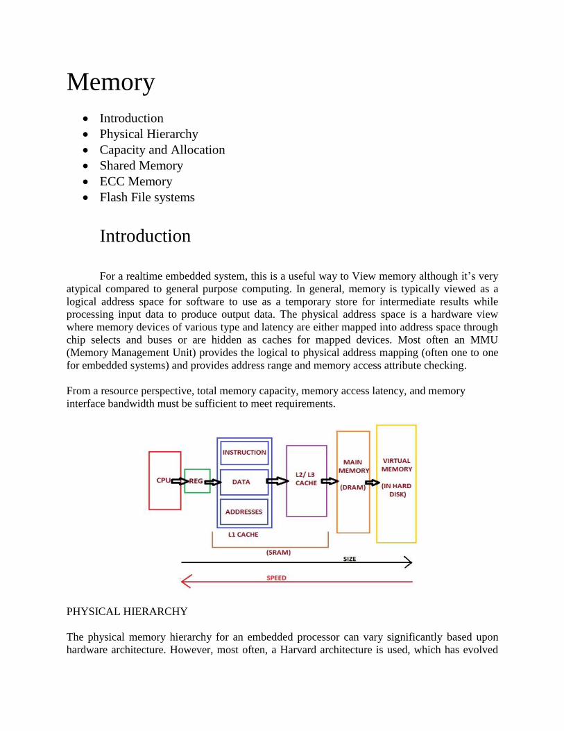
Memory

Introduction

Physical Hierarchy

Capacity and Allocation

Shared Memory

ECC Memory

Flash File systems

Introduction

For a realtime embedded system, this is a useful way to View memory although it’s very

atypical compared to general purpose computing. In general, memory is typically viewed as a

logical address space for software to use as a temporary store for intermediate results while

processing input data to produce output data. The physical address space is a hardware view

where memory devices of various type and latency are either mapped into address space through

chip selects and buses or are hidden as caches for mapped devices. Most often an MMU

(Memory Management Unit) provides the logical to physical address mapping (often one to one

for embedded systems) and provides address range and memory access attribute checking.

From a resource perspective, total memory capacity, memory access latency, and memory

interface bandwidth must be sufficient to meet requirements.

PHYSICAL HIERARCHY

The physical memory hierarchy for an embedded processor can vary significantly based upon

hardware architecture. However, most often, a Harvard architecture is used, which has evolved

from GPCs (general purpose computers) and is often employed by embedded systems as well.

The typical Harvard architecture with separate L1 (Level 1) instruction and data caches, but with

unified L2 (Level 2)cache and either on chip SRAM or external DDR (Dynamic Data RAM).

From the software viewpoint, memory is a global resource in a single address space with all

other MMIO as shown below.

Memory system design has been most influenced by GPC architecture and goals to maximize

throughput, but not necessarily to minimize the latency for any single memory access or

operation. The multilevel cached memory hierarchy for GPC platforms now often includes

Harvard L1 and unified L2 caches on chip width off chip L3 unified cache. The caches for GPCS

are most often set associative with aging bits for each cache set (line) so that the LRU (Least

Recently Used) sets are replaced when a cache line must be loaded. An N way set associative

cache can load an address reference into any N ways in the cache allowing for the LRU line to

be replaced. The LRU replacement policy, or approximation thereof, leads to a high cache hit to

miss ratio so that a processor most often finds data in cache and does not have to suffer the

penalty of a cache miss. The set associative cache is a compromise between a direct mapped a

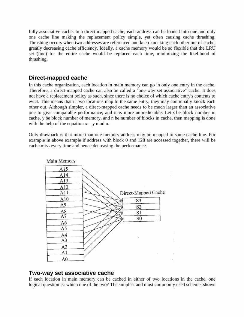
fully associative cache. In a direct mapped cache, each address can be loaded into one and only

one cache line making the replacement policy simple, yet often causing cache thrashing.

Thrashing occurs when two addresses are referenced and keep knocking each other out of cache,

greatly decreasing cache efficiency. Ideally, a cache memory would be so flexible that the LRU

set (line) for the entire cache would be replaced each time, minimizing the likelihood of

thrashing.

Direct-mapped cache In this cache organization, each location in main memory can go in only one entry in the cache.

Therefore, a direct-mapped cache can also be called a "one-way set associative" cache. It does

not have a replacement policy as such, since there is no choice of which cache entry's contents to

evict. This means that if two locations map to the same entry, they may continually knock each

other out. Although simpler, a direct-mapped cache needs to be much larger than an associative

one to give comparable performance, and it is more unpredictable. Let x be block number in

cache, y be block number of memory, and n be number of blocks in cache, then mapping is done

with the help of the equation x = y mod n.

Only drawback is that more than one memory address may be mapped to same cache line. For

example in above example if address with block 0 and 128 are accessed together, there will be

cache miss every time and hence decreasing the performance.

Two-way set associative cache If each location in main memory can be cached in either of two locations in the cache, one

logical question is: which one of the two? The simplest and most commonly used scheme, shown

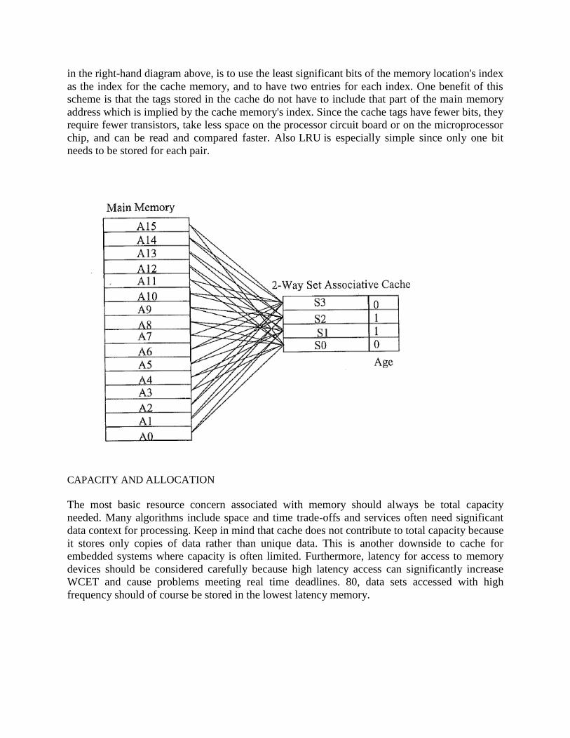
in the right-hand diagram above, is to use the least significant bits of the memory location's index

as the index for the cache memory, and to have two entries for each index. One benefit of this

scheme is that the tags stored in the cache do not have to include that part of the main memory

address which is implied by the cache memory's index. Since the cache tags have fewer bits, they

require fewer transistors, take less space on the processor circuit board or on the microprocessor

chip, and can be read and compared faster. Also LRU is especially simple since only one bit

needs to be stored for each pair.

CAPACITY AND ALLOCATION

The most basic resource concern associated with memory should always be total capacity

needed. Many algorithms include space and time trade-offs and services often need significant

data context for processing. Keep in mind that cache does not contribute to total capacity because

it stores only copies of data rather than unique data. This is another downside to cache for

embedded systems where capacity is often limited. Furthermore, latency for access to memory

devices should be considered carefully because high latency access can significantly increase

WCET and cause problems meeting real time deadlines. 80, data sets accessed with high

frequency should of course be stored in the lowest latency memory.

SHARED MEMORY

Shared memory is a way of inter-process communication where processes share a single lump of

physical memory space. The memory space is the resource pool for the processes from where the

processes are allocated resources according to some predefined algorithms.

Shared memory is a method by which program processes can exchange data more quickly than

by reading and writing using the regular operating system services. For example, a client process

may have data to pass to a server process that the server process is to modify and return to the

client. Ordinarily, this would require the client writing to an output file (using the buffers of the

operating system) and the server then reading that file as input from the buffers to its own work

space. Using a designated area of shared memory, the data can be made directly accessible to

both processes without having to use the system services. To put the data in shared memory, the

client gets access to shared memory after checking a semaphore value, writes the data, and then

resets the semaphore to signal to the server (which periodically checks shared memory for

possible input) that data is waiting. In turn, the server process writes data back to the shared

memory area, using the semaphore to indicate that data is ready to be read.

Clearly if the Update Code was interrupted and preempted by the Read Code at line 4 for

example, then the contro1(X, Y, 2) function would be using the new X and possibly an incorrect

and definitely old Y and 2. However, the semTake(Semid) and semGive(Semid) guarantee that

the Read Code cant preempt the Update Code no matter what the RM policies are. How does it

do this? The semTake(Semid) is a TSL instruction (Test and Set Lock< n ) a single cycle,

supported by hardware, the Semid memory location is first tested to see if it is 0 or 1. If 1, set to

0, and execution continues; if Semid is 0 on the test, the Value of Semid is unchanged, and the

next instruction is a branch to a wait queue and CPU yield. Whenever a service does a semGive

(Semid ) , the wait queue is checked and the first waiting service is unblocked. The unblocking is

achieved by dequeuing the waiting service from the wait queue and then placing it on the ready

queue for execution inside the critical section at its normal priority.

ECC memory

Error-correcting code memory (ECC memory) is a type of computer data storage that can detect

and correct the most common kinds of internal data corruption. ECC memory is used in most

computers where data corruption cannot be tolerated under any circumstances, such as for

scientific or financial computing.

The memory only has to store the parity or ECC bits, just as it stores the data bits. Parity is

implemented on most PCs with one parity bit per byte. For a 32-bit word size there are four

parity bits, for a total of 36 bits that have to be stored in the memory. On most Pentium and

Pentium Pro systems, and a few 486 systems, there is a 64-bit wide memory data path, so there

are eight parity bits, for a total of 72 bits.

When a word is written into memory, each parity bit is generated from the data bits of the byte it

is associated with. This is done by a tree of exclusive-or gates. When the word is read back from

the memory, the same parity computation is done on the data bits read from the memory, and the

result is compared to the parity bits that were read. Any computed parity bit that doesn't match

the stored parity bit indicates that there was at least one error in that byte (or in the parity bit

itself). However, parity can only detect an odd number of errors. If an even number of errors

occur, the computed parity will match the read parity, so the error will go undetected. Since

memory errors are rare if the system is operating correctly, the vast majority of errors will be

single-bit errors, and will be detected.

Unfortunately, while parity allows for the detection of single bit errors, it does not provide a

means of determining which bit is in error, which would be necessary to correct the error. This is

why parity is only an Error Detection Code (EDC).

ECC is an extension of the parity concept. ECC is usually performed only on complete words,

rather than individual bytes. In a typical ECC system with a 64-bit data word, there would be 7

ECC bits. Each ECC bit is calculated as the parity of a different subset of the data bits. The key

to the power of ECC is that each data bit contributes to more than one ECC bit. By making

careful choices as to which data bits contribute to which ECC bits, it becomes possible to not just

detect a single-bit error, but actually identify which bit is in error (even if it is one of the ECC

bits). In fact, the code is usually designed so that single-bit errors can be corrected, and double-

bit errors can be detected (but not corrected), hence the term Single Error Correction with

Double Error Detection (SECDED).

When a word is written into ECC-protected memory, the ECC bits are computed by a set of

exclusive-or trees. When the word is read back, the exclusive-OR trees use the data read from the

memory to re-compute the ECC. The recomputed ECC is compared to the ECC bits read from

the memory. Any discrepancy indicates an error. By looking at which ECC bits don't match, it is

possible to identify which data or ECC bit is in error, or whether a double-bit error occurred. In

practice this comparison is done by an exclusive-or of the read and recomputed ECC bits. The

result of this exclusive-or is called the syndrome. If the syndrome is zero, no error occurred. If

the syndrome is non-zero, it can be used to index a table to determine which bits are in error, or

that the error is uncorrectable. This table lookup stage is implemented in hardware in some

systems, and via an interrupt, trap, or exception in others. In the latter case, the system software

is responsible for correcting the error if possible.

FLASH FILE SYSTEM en.wikipedia.org

Flash memory is a memory storage device for computers and electronics. It is most often used in

devices like digital cameras, USB flash drives, and video games. It is quite similar to

EEPROM. Flash memory is different from RAM because RAM is volatile (not permanent).

When power is turned off, RAM loses all its data.

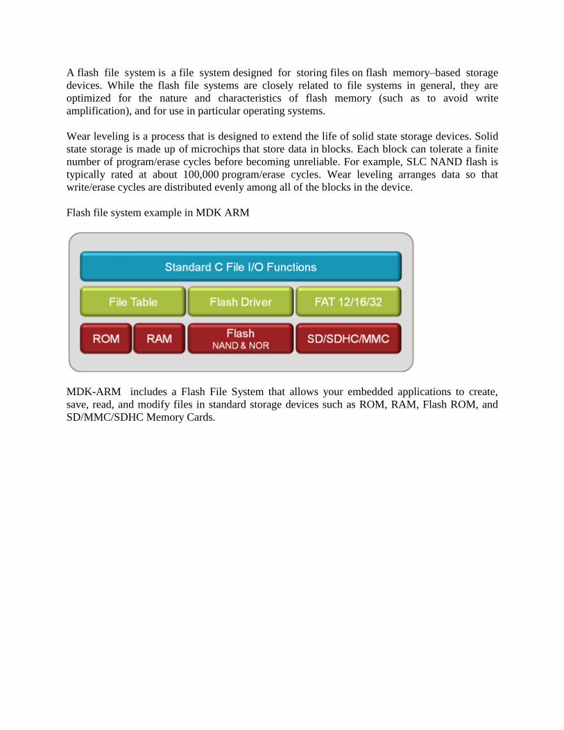
A flash file system is a file system designed for storing files on flash memory–based storage

devices. While the flash file systems are closely related to file systems in general, they are

optimized for the nature and characteristics of flash memory (such as to avoid write

amplification), and for use in particular operating systems.

Wear leveling is a process that is designed to extend the life of solid state storage devices. Solid

state storage is made up of microchips that store data in blocks. Each block can tolerate a finite

number of program/erase cycles before becoming unreliable. For example, SLC NAND flash is

typically rated at about 100,000 program/erase cycles. Wear leveling arranges data so that

write/erase cycles are distributed evenly among all of the blocks in the device.

Flash file system example in MDK ARM

MDK-ARM includes a Flash File System that allows your embedded applications to create,

save, read, and modify files in standard storage devices such as ROM, RAM, Flash ROM, and

SD/MMC/SDHC Memory Cards.

Multiresource Services

Introduction

Blocking

Deadlock and Livelock

Critical Sections to Protect Shared Resources

Priority Inversion

Power Management and Processor Clock Modulation

Introduction

Many services may need mutually exclusive access to shared memory resources or a shared

intermediate I/O resource. If this resource is not in use by another service, this presents no

problem. However, if a service is released and preempts another running service based upon RM

policy, only to find that it lacks a resource held by another service, then it is blocked. When a

service is blocked, it must yield" the CPU despite the RM policy.

BLOCKING

Blocking occurs anytime a service can be dispatched by the CPU, but isn’t because it is lacking

some other resource such as access to a shared memory critical section or access to a bus. When

blocking has a known latency, it could simply be added into response time, accounted for, and

therefore would not adversely affect RM analysis, although it would complicate it. The bigger

concern is unbounded blocking, where the amount of time a service will be blocked awaiting a

resource is indefinite or at least hard to calculate. Three phenomena related to resource sharing

can cause this: deadlock, live lock, and unbounded priority inversion. Deadlock and live lock are

always unbounded by definition. Priority inversion can be temporary, but under certain

conditions, priority inversion can be indefinite.

Blocking can be extremely dangerous because it can cause a much underutilized system to miss

deadlines. This is counter intuitive how can systems with only 5% CPU loading miss deadlines?

If a service is blocked for an indefinite time, then the CPU is yielded for an indefinite time,

leaving plenty of CPU margin, but the service fails to produce a response by its deadline.

DEADLOCK AND LIVELOCK

In Figure below, service S1needs resources A and C, 82 needs A and B, and S3needs B and C. If

S, acquires A, then S2acquires B, then S3acquires C followed by requests by each for their other

required resource, a circular wait evolves as shown in Figure 6.1. Circular wait, also known as

the deadly embrace, causes indefinite deadlock. No progress can be made by Services 1, 2, or 3

in Figure 6.1 unless resources held by each are released. Deadlock can be prevented by making

sure the circular wait scenario is impossible, “High Availability and Reliability Design When the

keep alive is not posted due to the deadlock, then a supervisory service can restart the

deadlocked service. However, it’s possible that when deadlock is detected and services are

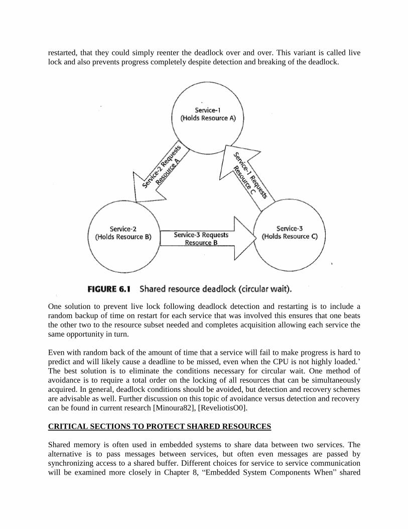
restarted, that they could simply reenter the deadlock over and over. This variant is called live

lock and also prevents progress completely despite detection and breaking of the deadlock.

One solution to prevent live lock following deadlock detection and restarting is to include a

random backup of time on restart for each service that was involved this ensures that one beats

the other two to the resource subset needed and completes acquisition allowing each service the

same opportunity in turn.

Even with random back of the amount of time that a service will fail to make progress is hard to

predict and will likely cause a deadline to be missed, even when the CPU is not highly loaded.’

The best solution is to eliminate the conditions necessary for circular wait. One method of

avoidance is to require a total order on the locking of all resources that can be simultaneously

acquired. In general, deadlock conditions should be avoided, but detection and recovery schemes

are advisable as well. Further discussion on this topic of avoidance versus detection and recovery

can be found in current research [Minoura82], [ReveliotisO0].

CRITICAL SECTIONS TO PROTECT SHARED RESOURCES

Shared memory is often used in embedded systems to share data between two services. The

alternative is to pass messages between services, but often even messages are passed by

synchronizing access to a shared buffer. Different choices for service to service communication

will be examined more closely in Chapter 8, “Embedded System Components When” shared

memory is used, because real-time systems allow for event driven preemption of services by

higher priority service releases at any time, shared resources such as shared memory must be

protected to ensure mutually exclusive access. So, if one service is updating a shared memory

location (writing), it must fully complete the update before another service is allowed to preempt

the writer and read the same location as described already in Chapter 4. If this mutex (mutually

exclusive access) to the update/read data is not enforced, then the reader might read a partially

updated message. If the code for each service that either updates or reads the shared data is

surrounded with a semTake () and semGive () (in Vx Work for example), then the update and

read will be uninterrupted despite the preemptive nature of the RTOS scheduling. The first caller

to semTake() will enter the critical update section, but the second caller will be blocked and not

allowed to enter the partially updated data, causing the original service in the critical section to

always fully update or read the data. When the current user of the critical section calls semGive

() upon leaving the critical section, the service blocked on the semTake () is then allowed to

continue safely into the critical section. The need and use of semaphores to protect such shared

resources is a well understood concept in multithreaded operating systems.

PRIORITY INVERSION

Priority inversion is simply defined as any time that a high priority service has to wait while a

lower priority service runs this can occur in any blocking scenario. We’re most concerned about

unbounded priority inversion. If the inversion is bounded, then this can be lumped into the

response latency and accounted for so that the RM analysis is still possible. The use of any

mutex (mutual exclusion) semaphore can cause a temporary inversion while a higher priority

service is blocked to allow a lower priority service to complete a shared memory read or update

in its entirety. As long as the lower priority service executes for a critical section WCET, the

inversion is known to last no longer than the lower priority service’s WCET for the critical

section. What causes unbounded priority inversion? Three conditions are necessary for

unbounded inversion:

Three or more services with unique priority in the system High(H), Medium (M), Low

(L) priority sets of services.

At least two services of different priority share a resource with mutex protection one or

more high and one or more low involved.

One or more services not involved in the mutex has priority between the two involved in

the mutex.

Essentially, a member of the H priority service set catches an L priority service in the critical

section and is blocked on the semTake (semid). While the L priority service executes in the

critical section, one or more M priority services interfere with the L priority service’s progress

for an indefinite amount of time; the H priority service must continue to wait not only for the L

priority service to finish the critical section, but for the duration of all interference to the L

priority service. How long will this interference go on? This would be hard to put an upper

bound on clear it could be longer than the deadline for the H priority service. Figure 6.2 depicts a

shared memory usage scenario for a spacecraft system that has two services using or calculating

navigational data providing the vehicles position and attitude in inertial space; one service is a

low priority thread of execution that periodically points an instrument based upon position and

attitude at a target planet to look for a landing site. A second service, running a high priority, is

using basic navigational sensor readings and computed trajectory information to update the best

estimate of the current navigational state. In Figure 6.2, a set of M priority services {M}that are

unrelated to the shared memory data critical section can cause H to block for as long as M

services continue to preempt the L service stuck in the critical section.

Unbounded Priority Inversion Solutions

One of the first solutions to unbounded priority inversion is to use task or interrupt locking (Vx

Works intLock ( ) and intUnlock ( ) or task Lock () and task Unlock () to prevent preemptions in

critical sections completely, which operates in the same way as a priority ceiling protocol.

Priority inheritance was introduced as a more optimal method that limits the amplification of

priority in a critical section only to the level required to bound inversions. By comparison,

interrupt locking and priority ceiling essentially disable all preemption for the duration of the

critical section, but very effectively bound the inversion. To describe better what is meant by

priority inheritance, you must understand the basic strategy to avoid indefinite interference while

a low priority task is in a critical section. Basically, the H priority service gives its priority

temporarily to the L priority service so that it will not be preempted by the M priority services

while finishing up the critical section normally priority service restores the priority loaned to it as

soon as it leaves the critical section.

The priority of the L service is temporarily amplifier to the H priority to prevent the unbounded

inversion. One downside to priority inheritance is that it can chain. When H blocks, it is possible

that shortly after H loans its priority to L, another H+n priority service will block on the same

semaphore, therefore requiring a new inheritance of H+n by L so that H+n is not blocked by

services of priority H+1 to H+n—1 interfering with L, which has priority H. The chaining is

complex, so it would be easier to simply give L a priority that is so high that chaining is not

necessary. This idea became the priority ceiling emulation protocol (also known as highest

locker).

A further refinement of priority ceiling is the least locker protocol. In least locker, the priority of

L is amplified to the highest priority of all those services that can potentially request access to

the critical section. The only downside to least, locker is that it requires the programmer to

indicate to the operating system what the least locker priority should be. Any mistake in

specification to the of least lock priority may cause unbounded inversion. In theory, the

programmer should know very well what services can enter a given critical section and therefore

also know the correct least locker priority.

The problem of priority inversion became famous with the Mars Pathfinder spacecraft. The

Pathfinder spacecraft was on final approach to Mars and would need to complete a critical

engine burn to capture into a Martian orbit within a few days after a cruise trajectory lasting

many months. The mission engineers readied the craft by enabling new services. Services such

as meteorological processing from instruments were designed to help determine the insertion

orbit around Mars because one of the objectives of the mission was to land the Sojourner rover

on the surface in a location free of dangerous dust storms. When the new services were activated

during this critical final approach, the Pathfinder began to reboot when one of the highest priority

services failed to service the hardware watch dog timer.

Reasons for a watch dog timer could include the following:

Deadlock or live lock preventing the watch dog timer service from executing

Loss of software sanity due to programming errors such as a bad pointer, an improperly

handled processor exception, such as divide by zero, or a bus error

Overload due to miscalculation of WCETs for the final approach service set

A hardware malfunction of the watch dog timer or associated circuitry

A multibit error in memory due to space radiation causing a bit upset

Most often, the reason for reset is stored in a nonvolatile memory that is persistent through a

watch dog timer so that exceptions due to programming errors, memory bit upsets, and hardware

malfunctions would be apparent as the reason for reset and/or through anomalies in system

health and status telemetry.

After analysis on the ground using a test—bed with identical hardware and data play back along

with analysis of code, it was determined that Pathfinder might be suffering from priority

inversion. Ideally, a theory like this would be validated first on the ground in the testbed by

recreating conditions to verify that the suspected bug could cause the observed behavior. Priority

inversion was suspected because a message passing method in the Vx Works RTOS used by

firmware developers was found to ultimately use shared memory with an option bit for priority,

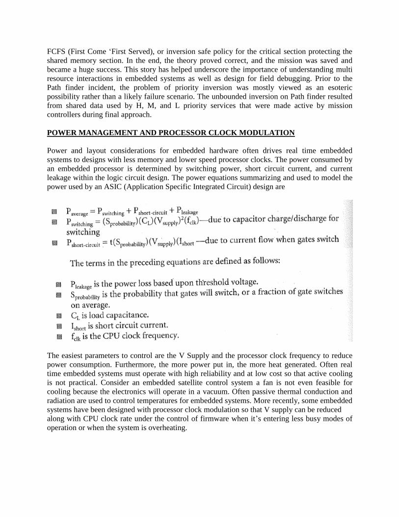
FCFS (First Come ‘First Served), or inversion safe policy for the critical section protecting the

shared memory section. In the end, the theory proved correct, and the mission was saved and

became a huge success. This story has helped underscore the importance of understanding multi

resource interactions in embedded systems as well as design for field debugging. Prior to the

Path finder incident, the problem of priority inversion was mostly viewed as an esoteric

possibility rather than a likely failure scenario. The unbounded inversion on Path finder resulted

from shared data used by H, M, and L priority services that were made active by mission

controllers during final approach.

POWER MANAGEMENT AND PROCESSOR CLOCK MODULATION

Power and layout considerations for embedded hardware often drives real time embedded

systems to designs with less memory and lower speed processor clocks. The power consumed by

an embedded processor is determined by switching power, short circuit current, and current

leakage within the logic circuit design. The power equations summarizing and used to model the

power used by an ASIC (Application Specific Integrated Circuit) design are

The easiest parameters to control are the V Supply and the processor clock frequency to reduce

power consumption. Furthermore, the more power put in, the more heat generated. Often real

time embedded systems must operate with high reliability and at low cost so that active cooling

is not practical. Consider an embedded satellite control system a fan is not even feasible for

cooling because the electronics will operate in a vacuum. Often passive thermal conduction and

radiation are used to control temperatures for embedded systems. More recently, some embedded

systems have been designed with processor clock modulation so that V supply can be reduced

along with CPU clock rate under the control of firmware when it’s entering less busy modes of

operation or when the system is overheating.

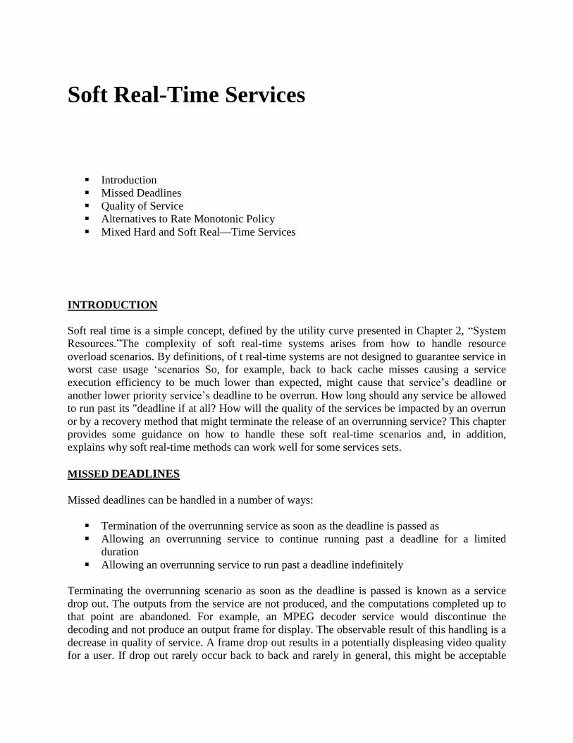
Soft Real-Time Services

Introduction

Missed Deadlines

Quality of Service

Alternatives to Rate Monotonic Policy

Mixed Hard and Soft Real—Time Services

INTRODUCTION

Soft real time is a simple concept, defined by the utility curve presented in Chapter 2, “System

Resources.”The complexity of soft real-time systems arises from how to handle resource

overload scenarios. By definitions, of t real-time systems are not designed to guarantee service in

worst case usage ‘scenarios So, for example, back to back cache misses causing a service

execution efficiency to be much lower than expected, might cause that service’s deadline or

another lower priority service’s deadline to be overrun. How long should any service be allowed

to run past its "deadline if at all? How will the quality of the services be impacted by an overrun

or by a recovery method that might terminate the release of an overrunning service? This chapter

provides some guidance on how to handle these soft real-time scenarios and, in addition,

explains why soft real-time methods can work well for some services sets.

MISSED DEADLINES

Missed deadlines can be handled in a number of ways:

Termination of the overrunning service as soon as the deadline is passed as

Allowing an overrunning service to continue running past a deadline for a limited

duration

Allowing an overrunning service to run past a deadline indefinitely

Terminating the overrunning scenario as soon as the deadline is passed is known as a service

drop out. The outputs from the service are not produced, and the computations completed up to

that point are abandoned. For example, an MPEG decoder service would discontinue the

decoding and not produce an output frame for display. The observable result of this handling is a

decrease in quality of service. A frame drop out results in a potentially displeasing video quality

for a user. If drop out rarely occur back to back and rarely in general, this might be acceptable

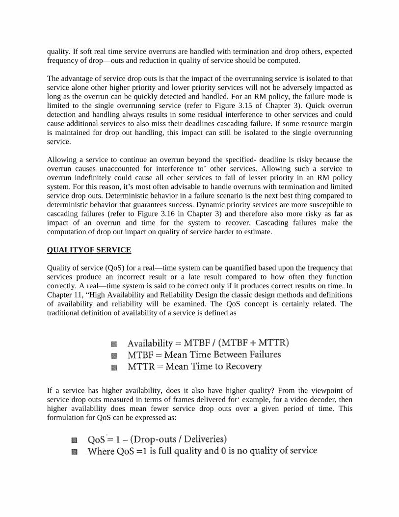
quality. If soft real time service overruns are handled with termination and drop others, expected

frequency of drop—outs and reduction in quality of service should be computed.

The advantage of service drop outs is that the impact of the overrunning service is isolated to that

service alone other higher priority and lower priority services will not be adversely impacted as

long as the overrun can be quickly detected and handled. For an RM policy, the failure mode is

limited to the single overrunning service (refer to Figure 3.15 of Chapter 3). Quick overrun

detection and handling always results in some residual interference to other services and could

cause additional services to also miss their deadlines cascading failure. If some resource margin

is maintained for drop out handling, this impact can still be isolated to the single overrunning

service.

Allowing a service to continue an overrun beyond the specified- deadline is risky because the

overrun causes unaccounted for interference to’ other services. Allowing such a service to

overrun indefinitely could cause all other services to fail of lesser priority in an RM policy

system. For this reason, it’s most often advisable to handle overruns with termination and limited

service drop outs. Deterministic behavior in a failure scenario is the next best thing compared to

deterministic behavior that guarantees success. Dynamic priority services are more susceptible to

cascading failures (refer to Figure 3.16 in Chapter 3) and therefore also more risky as far as

impact of an overrun and time for the system to recover. Cascading failures make the

computation of drop out impact on quality of service harder to estimate.

QUALITYOF SERVICE

Quality of service (QoS) for a real—time system can be quantified based upon the frequency that

services produce an incorrect result or a late result compared to how often they function

correctly. A real—time system is said to be correct only if it produces correct results on time. In

Chapter 11, “High Availability and Reliability Design the classic design methods and definitions

of availability and reliability will be examined. The QoS concept is certainly related. The

traditional definition of availability of a service is defined as

If a service has higher availability, does it also have higher quality? From the viewpoint of

service drop outs measured in terms of frames delivered for‘ example, for a video decoder, then

higher availability does mean fewer service drop outs over a given period of time. This

formulation for QoS can be expressed as:

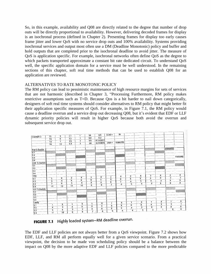
So, in this example, availability and Q08 are directly related to the degree that number of drop

outs will be directly proportional to availability. However, delivering decoded frames for display

is an isochronal process (defined in Chapter 2). Presenting frames for display too early causes

frame jitter and lower QoS with no service drop outs and 100% availability. Systems providing

isochronal services and output most often use a DM (Deadline Monotonic) policy and buffer and

hold outputs that are completed prior to the isochronal deadline to avoid jitter. The measure of

QoS is application specific. For example, isochronal networks often define QoS as the degree to

which packets transported approximate a constant bit rate dedicated circuit. To understand QoS

well, the specific application domain for a service must be well understood. In the remaining

sections of this chapter, soft real time methods that can be used to establish Q08 for an

application are reviewed.

ALTERNATIVES TO RATE MONOTONIC POLICY

The RM policy can lead to pessimistic maintenance of high resource margins for sets of services

that are not harmonic (described in Chapter 3, “Processing Furthermore, RM policy makes

restrictive assumptions such as T=D. Because Qos is a bit harder to nail down categorically,

designers of soft real time systems should consider alternatives to RM policy that might better fit

their application specific measures of QoS. For example, in Figure 7.1, the RM policy would

cause a deadline overrun and a service drop out decreasing Q08, but it’s evident that EDF or LLF

dynamic priority policies will result in higher QoS because both avoid the overrun and

subsequent service drop out.

The EDF and LLF policies are not always better from a QoS viewpoint. Figure 7.2 shows how

EDF, LLF, and RM all perform equally well for a given service scenario. From a practical

viewpoint, the decision to be made von scheduling policy should be a balance between the

impact on Q08 by the more adaptive EDF and LLF policies compared to the more predictable

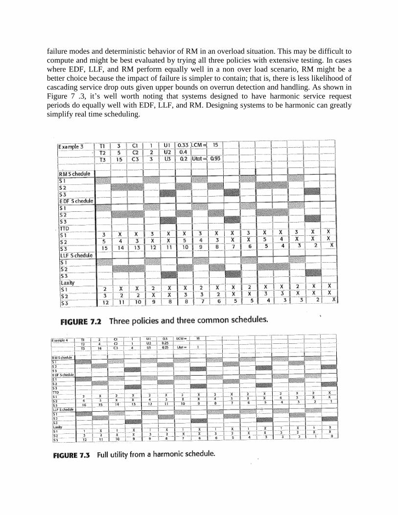
failure modes and deterministic behavior of RM in an overload situation. This may be difficult to

compute and might be best evaluated by trying all three policies with extensive testing. In cases

where EDF, LLF, and RM perform equally well in a non over load scenario, RM might be a

better choice because the impact of failure is simpler to contain; that is, there is less likelihood of

cascading service drop outs given upper bounds on overrun detection and handling. As shown in

Figure 7 .3, it’s well worth noting that systems designed to have harmonic service request

periods do equally well with EDF, LLF, and RM. Designing systems to be harmonic can greatly

simplify real time scheduling.

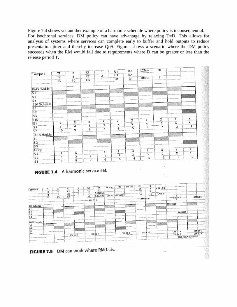
Figure 7.4 shows yet another example of a harmonic schedule where policy is inconsequential.

For isochronal services, DM policy can have advantage by relaxing T=D. This allows for

analysis of systems where services can complete early to buffer and hold outputs to reduce

presentation jitter and thereby increase QoS. Figure shows a scenario where the DM policy

succeeds when the RM would fail due to requirements where D can be greater or less than the

release period T.

MIXED HARD AND SOFT REAL-TIME SERVICES

Many systems include services that are hard real time, soft real time, and best effort. For

example, a computer vision system on an assembly line may have hard real time services where

missing a deadline would cause shutdown of the process being controlled. Likewise, operators

may want to occasionally monitor what the computer vision systems “sees.”The video for

monitoring should have good Q08so that a human monitor can assess how well the system is

working, whether lighting is sufficient and’ whether frame rates appear reasonable. Finally, in

the same system, operators may occasionally want to dump maintenance data and have no real

requirements for how fast this is done it can be done in the background whenever spare cycles

are available.

The mixing of hard, soft, and best effort can be done by admitting the services into multiple

periodic servers for each. The hard real—time services can be scheduled within a time period

(epoch) during which the CPU is dedicated only to hard real time services (all others are

preempted). Another approach is to period transforming all the hard real—time services so that

they have priorities that encode their importance. Either way, we ensure that the hard real—time

services will preempt all soft services and best effort services on a deterministic and periodic

basis.

Best effort services can always be handled by simply scheduling all these services at the lowest

priority and at an equal priority among them. At lowest priority, best—effort services become

slack time stealers that execute only when no real—time (hard or soft) services are requesting

processor resources.