A discrete-time multiresolution theory - Signal Processing

I I

2591 IEEE TRANSACTIONS ON SIGNAL PROCESSING, VOL. 41. NO. 8, AUGUST 1993

A Discrete-Time Multiresolution Theory Olivier Rioul

Abstract-Multiresolution analysis and synthesis for discrete- time signals is described in this paper. Concepts of scale and resolution are first reviewed in discrete time. The resulting framework allows one to treat the discrete wavelet transform, octave-band perfect reconstruction filter banks, and pyramid transforms from a unified standpoint. This approach is very close to previous work on multiresolution decomposition of functions of a continuous variable, and the connection between these two approaches is made. We show that they share many mathematical properties such as biorthogonality, orthonormality, and regularity. However, the discrete-time formalism is well suited to practical tasks in digital signal processing and does not require the use of functional spaces as an intermediate step.

I. INTRODUCTION AVELET transforms [21], octave-band filter banks w [23], [24], and pyramid transforms [3] have been

used for different purposes in various fields of signal processing; they are now recognized as different views of a common theory. ’ This paper establishes the links between these techniques for discrete-time signals, focusing on basis decomposition in time rather than frequency decomposition. This topic is close to the one studied in a recent work by Shensa [22] that clarifies the relationship of various discrete-time and continuous-time wavelet transforms using a similar formalism. While [22] focuses on implementation issues of the “continuous wavelet transform” (to be defined below) for signal analysis purposes, we consider only a discrete-time version of the wavelet transform that is more appropriate for coding applications. We assume one-dimensional signals; extension to more dimensions may not be straightforward [25], but the ideas are the same as in one dimension.

There are various types of wavelet transforms, for which the connection to filter banks is more or less ob- vious. The continuous wavelet transform (CWT) is the first type of wavelet transform defined in the literature [ 121. It maps a one-dimensional analog signal n (t) to a set of wavelet coefficients which vary continuously over time b and scale a:

CWT (a, b) = U - ‘ / * ~ ( t ) $* ( t a - ’) dt.

Manuscript received June 26, 1990; revised September 21, 1992. The associate editor coordinating the review of this paper and approving it for publication was Prof. Faye Boudreaux-Bartels.

The author is with the Centre National d’Etudes des T61Bcommunica- tions, CNET/PAB/RPE/ETP, 9213 1 Issy-Les-Moulineaux, France.

IEEE Log Number 9209395. ’The reader is referred to [21] and [24) for tutorial descriptions of mul-

tiresolution theory and multirate filter banks, and to 181, [151-[171 for a mathematical study of wavelets.

The “wavelet” functions +((t - b) /a ) are used to band- pass filter the signal. This can be seen as a kind of time- varying spectral analysis in which scale a plays the role of a local frequency: As a increases, wavelets are stretched and analyze low frequencies, while for small a, contracted wavelets analyze high frequencies. Therefore, the time-frequency extents of the wavelets vary according to a “constant-Q ” scheme [21], with various resolutions in time or frequency (multiresolution analysis), whereas techniques based on short-time Fourier transforms analyze the signal at constant resolution [21].

In applications such as signal coding or compression, time-scale parameters (b, a) are sampled, so that the signal is represented by wavelet coefficients in an economical manner. A typical choice is a = 2J, J E 2 (octave by octave computation [2 11); in addition, wavelets are shifted in proportion to their temporal extent, i.e., b = k2’. Wavelet ‘‘basic functions” become

and wavelet coefficients are inner products of the signal with the $j,k(t)’S,

(3)

Note that this “sampled” wavelet transform still applies to continuous-time (analog) signals. It has been extensively studied by Meyer [17] and Mallat [15], [16] who built a complete mathematical theory based on “multiresolution spaces” of functions. In fact, some of the ideas behind the theory were already found in image coding and computer vision [l], [3]. Based on this theory, several authors [4], [8], [9], [ 171 constructed special wavelet pro- totypes $ (t) for which perfect reconstruction of the signal x ( t ) is possible; the synthesis takes the form of a “wavelet series, ’ ’

(4)

where the synthesis wavelets $j,k (t) are defined similarly as (2) with wavelet prototype $(t). As a special case, orthonormal wavelets are obtained if one has $( t ) = +(t) .

In order that the coefficients (3) be computed effi- ciently, Mallat [15] derived a iterative algorithm that was transposed to compute the reconstruction part. Mallat’s direct and inverse algorithms turn out to be exactly an analysis and synthesis octave-band filter bank [23], [24], which is used on discrete-time signals. Filter bank theory is therefore closely related to wavelets. The former has

1053-587X/93$03.00 0 1993 IEEE

As

I

2592 IEEE TRANSACTIONS ON SIGNAL PROCESSING, VOL. 41, NO. 8, AUGUST 1993

been previously developed for applications such as subband coding of speech [7] or images [25], and has greatly influenced the latter. In fact, known FIR filter design techniques [23] were independently used by Daubechies [8], [9] to construct finite-length orthonormal wavelets; her construction is based on the classical MAXFLAT digital filters [13] which have been recently related to La- grangian interpolators [22] . Recently, FIR filter design methods were developed [4], [26] to construct linear phase, “biorthogonal” wavelets for which $ ( t ) # $ ( t ) .

Therefore, the connection between wavelet series and filter banks has been extensively studied. However, the “discrete-time side” of wavelet series was mainly considered as a technical step either for the derivation of fast algorithms which rely on the filter bank structure (for further developments see, e.g., [20]) or for the construction of continuous-time wavelet bases via filter design [4], [8], [9], [26]. On the other hand, filter banks were studied from the viewpoint of subband decomposition, which masks the time decomposition properties. In this paper, we focus on octave-band perfect reconstruction filter banks seen as multiresolution decomposition of discrete- time signals, performed by a discrete wavelet transform (DWT),2 to be defined in Section VII.

With the notable exception of Shensa [ 2 2 ] , very little can be found on this subject in the literature, in which it is generally admitted that analog wavelets are the interesting objects that underly discrete-time filter banks. Here, we adopt a dual point of view, and consider discrete wavelet transforms as the interesting objects. A discrete- time presentation of multiresolution theory may allow new developments; it is certainly more appropriate for practical tasks in digital signal processing than the continuous- time one. As an example, various image compression schemes were derived based on the wavelet model for analog signals [2], [27], but they are essentially discrete in nature.

This paper focuses on discrete-time signals and devel- ops a discrete-time multiresolution theory where ‘‘basis functions” on which the signal is decomposed are discrete-time wavelets. It is self-contained: the reader should not need to have previous knowledge on wavelets, although some rudimentary knowledge on vector spaces is assumed. Note that since the overlap between discrete- time and continuous-time approaches is important, the developments and ideas of this paper are known to wavelet experts, yet they do not appear in the literature as they are presented here.

11. NOTATIONS Throughout this paper we use the following notations.

Most of them are classical; in particular, the operator (or

’The acronym DWT is sometimes used to denote wavelet series decomposition of continuous-time signals (3) , (4). Here DWT refers to a type of wavelet transform which decomposes discrete-time signals, as in [22]. Al- though we shall see that the DWT reduces to an octave-band filter bank, we use the wavelet terminology to emphasize its multiresolution (time) decomposition properties, as opposed to the well-known subband (frequency) decomposition properties.

matrix) notations appear in other works (see, e.g., [8]) and have been reused by Shensa in [ 2 2 ] .

x or {x,> denotes the original signal, which is a discrete-time, complex-valued sequence. Its n th sample will be noted x,. 6 denotes the “pulse” signal, whose samples are 6,, = 1 and 6, = 0 if n # 0.

G and H denote the low-pass and high-pass filtering operator, respectively. The corresponding impulse responses are g, and h,. Therefore, Gx is a low-pass filtered signal, i.e., the result of the discrete convolution (Gx), = Ck X k g , - k . When needed, the sample index of the input is shown, as in (Gxk). Z is the identity operator, Zx = x, of impulse response 6.

t x and 1 x denote the upsampled and downsampled signals, respectively. They are defined by (t x ) ~ , = x,, (t x ) ~ , + , = 0, and (1 x), = x2,. Upscaled and downscaled signals, to be defined in Section 111, are denoted by G t x and 1 G’x, respectively.

The inner product of x with y is (x, y ) = (x,, y,) = E, x I I y ; . In particular, = (x, x ) is the squared norm of x.

111. SCALING IN DISCRETE TIME This section defines scale for discrete-time signals. This

definition is inspired from the commonly used scale of road maps: given a “real” object, the scale of a representation of this object is the ratio of the length unit of the representation to the corresponding real length. Here the “real object” is an original discrete-time signal {x,}, which is at scale 1 by definition, and scale refers to discrete time: a scaled version of {x,} is either 1) “upscaled”: a discrete-time signal similar to { x n ) , but sampled at a higher rate; or 2) “downscaled”: a discrete-time signal similar to {x,), but sampled at a lower rate.

Since scale is a relative notion, we focus on the description of scale-changing operators that map a signal into a scaled version of it. Throughout the paper we restrict to changes of scale by an integer power of two. We therefore study two basic scaling operators: 1) “upscaling” operator (by a factor 2): a discrete-time equivalent to the dilation x ( t ) -+ x ( t / 2 ) ; and 2) “downscaling” operator (by a factor 2): a discrete-time equivalent to the contraction x ( t ) + x(2t).

Obviously, the scale notion is related to multirate systems [6]. For example, a downscaled version of x, could be its downsampled version, (1 x), = x2,. However, upsampling (t x), = x,i2 if n is even, 0 otherwise, is not a good candidate for upscaling, since it inserts a zero between every other sample of x,, hence x and t x do not have similar evolutions in time. This can be corrected by further interpolating the samples, as in the following example, illustrated in Fig. 1:

Upscaled version of x,

RIOUL: DISCRETE-TIME MULTIRESOLUTION THEORY 2593

0 2 c 7 - I . . ’ - . . ’ ,----I

0 2 c ’ I

0 68 100

0 1 I 1

I . . . . . I . . . . I . .I I

0 68 I 0 0

Fig. 1. Two successive upscalings (by a factor 2) of an original discrete- time signal (top of figure). Upscaling is performed by first-order interpolation (5). Upscaled signals are stretched in time, but no resolution is added (see Section V).

In order to determine general expressions for up- and downscaling operators, we need some basic assumptions:

1) Scaling operators are linear. 2) When scaling a signal, time shifts are scaled ac-

cordingly. This is

If y, is the upscaled version of x,, then y , - 2k is the

If y , is the downscaled version of x,, then y, - k is the

3) Scaled versions have similar time evolutions (shape preservation). The third point is difficult to be properly expressed. It is not considered until Section X, where it is connected to the “regularity” property.

The first two assumptions result in the following char- acterizations, proven in Appendix A:

The upscaled version of x is of the form G t x , where G t denotes upsampling followed by filtering with some impulse response { g,} :

upscaled version of x, - k .

downscaled version of x, - 2k.

(G t x), = xkgn - 2 k . (6)

The downscaled version of x is of the form 1 G ’ x, where 1 G’ denotes filtering with some impulse response { g ; } , followed by downsampling:

(1 G ‘ X ) , = x x k g 4 n - k . (7) k

Note that the impulse responses { gn} and { g ; } are not necessarily equal. In the sequel, we assume that they are impulse responses of low-pass filters; intuitively this is required by assumption 3)-Section X gives a theoretical justification of it. As an example, ( 5 ) corresponds to a 3-tap upscaling filter g,, = 0.5, go = 1.

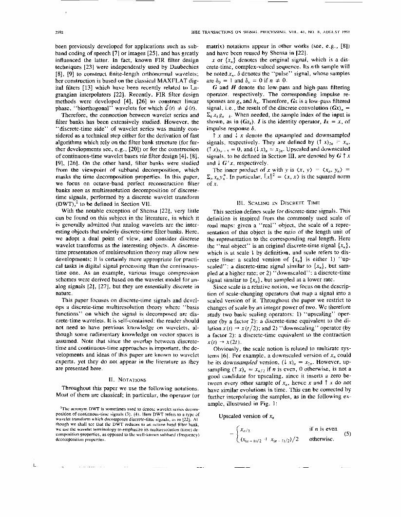
Of course, these up and down “scaling” operators are merely the usual interpolation and decimation operators present in a two-band filter bank [6], [23], [24]. (The corresponding flow graphs are shown in Fig. 2.) However, we keep using the “scale” terminology in the following because it is more appropriate for multiresolution decomposition of discrete-time signals. Note that the operator notation used here is very easily connected to flow-graph implementation; for example, G t 1 G ’ x means that the input x successively encounters a filter of impulse response g’ . , a downsampler, an upsampler, and finally a filter of impulse response g.

Now, using only these two operators (6), (7), one can compute scaled versions of the original signal {x,} at all dyadic scales s = 2-i, where i E 2. The rule is that the upscaling operator (6) doubles the scale, while the downscaling operator (7) halves it. Since the “scaling filters” { g,} and { g ; } remain fixed at all scales, all scale tran- sitions are performed the same way, and no particular scale is privileged. However, a scaled version of a given signal {x,} at some scale s is not unique. As an example, signals of the form (G t )N (1 G ’ ) M (G t)M (1 G ’ ) N ~ are all “scaled” versions of x at scale 1, for all nonnegative values of N and M. Therefore, to characterize scaled versions of n, we need another parameter, namely, resolution. which is defined in Section V.

IV. HERMITIAN TRANSPOSITION AND INNER PRODUCTS Before introducing the concept of resolution, it is con-

venient to say a few words about Hermitian transposition of operators and inner products. In matrix notation, the


8’. 4 e down - scaled version of x,

upscaling operator is [5] that transposing a linear operator amounts to transposing its flow graph: the Hermitian transposed flow graph is thus obtained by reversing the directions of all arrows- summing nodes become branching nodes and vice versu- and conjugating the multipliers. From the discussion above, it follows that the two flow graphs of Fig. 2 are

G t x = ( ...;; ;; ;; :; :;; ...) each other’s Hermitian transpose if and only if the scaling filters { g,,} and { g;} are each other’s paraconjugate (10). In any case, the flow-graph computational structures of up- and downscaling operators are always tranpose of each other. This has useful implications for deriving algorithms [20]; once an algorithm has been derived to compute downscaling, the transposed algorithm computes upscaling (and vice versa), at the same computational cost if both scaling filters have the same length. This easily carries over to direct and inverse wavelet transforms (see Section VI11 and [20]).

Another characterization of Hermitian transposition uses inner products and is useful in the sequel. The inner product of two discrete-time signals {x,} and { y , } can be

g4 g2 go g-2 g-4

* (j). Its Hermitian transpose is, by definition, the operator obtained from (8) by transposition and complex conjuga- tion, i.e., written

. ‘ . \

This is exactly the matrix form of a downscaling operator (7), with scaling filter { g ?,} in place of { g,} . Following the filter bank terminology [24], { g E,} is called the “paraconjugate” sequence of { g,} (the connection with filter banks will be explained in Section VIII). Paracon- jugation will be denoted in this paper with a tilde symbol:

g n = s*,. (10) We have thus seen that the Hermitian transpose of the upscaling op_erator G t is the paraconjugate downscaling operator 1 G. Similarly, the Hermitian transpose of the downscali_ng operator 1 G ’ is the paraconjugate upscaling operator G ’ t .

Hermitian transposition is useful for several reasons. First, it has a flow-graph interpretation: it is well known

This definition requires that signals have finite energy, i.e., llxll < 00, which is assumed throughout this paper. The inner product ( x , y ) measures the “similarity” between x and y and permits to interpret signals as geometric vectors: for example, the signals x and y are “orthogonal” if ( x , y ) = 0. They are “orthonormal” if they moreover have a unit norm, i.e., 1IxII = 1) yII = 1 . Using ( l l ) , it is easy to show that the Hermitian transpose Ot of some operator 0 can be alternatively defined as satisfying

( x , oy) = (O’X, y )

(x, 0% = (Ox, y )

(12)

or, equivalently,

(13)

RIOUL: DISCRETE-TIME MULTIRESOLUTION THEORY

for any signals x and y of finite energy. These equations do not introduce any new concept: only notations are new. They are useful because of their conciseness: any operator on the left-hand side of an inner product can be brought to the right-hand side after Hermitian transposition, and vice versa. For scaling operators we can thus write

(14)

(15) which, respectively, stand for the apparently more com- plicated formulas

( x , G t y ) = (1 G x , y )

( x , 1 G ’ y ) = ( G ’ t x , y )

and

To simplify notations, proofs in the Appendix will often use (14) and (15).

V . DISCRETE-TIME RESOLUTION A N D

BIORTHOGON ALITY

In this section we deflne the resolution notion for char- acterizing different versions of an original signal {x, ,} at the same scale. Intuitively, the more information is present in a scaled version of { x , } , the higher the resolution. More precisely, we define the resolution parameter r as follows: A scaled version of { x , } , obtained by action of up- and/or downscaling operators on { x , ] , is at resolution r = 2-/ ( j 1 0) if it is characterized by one sample every other 2’ sampling period of { x , } .

For example, x itself is at resolution 1. Its downscaled version 1 G ’ x (7), which lives at scale 1/2, is also at resolution 1 /2, because the downscaling operator rejects half of the samples. Note that in general, the resolution of a signal cannot exceed its scale, otherwise it would be characterized by more samples than are actually present in the signal. Therefore, we always have

r ( y ) 5 s ( y ) (16) for any signal y . Since we start from an original signal { x , } at resolution 1 , all resolutions considered in this paper are negative powers of two: r = 2 - / , j ? 0.

How is resolution affected by up and downscaling operators? We have seen that downscaling, when applied to the original signal { x , } , halves both scale and resolution. In contrast, since an upscaled signal is computed directly from the signal coefficients, resolution is not increased by up-scaling, which simply “magnifies” a signal without adding new details. Also, despite the low-pass filtering present in upscaling (6), information will not necessarily be lost when upscaling a signal. This is clear in the example (5) . We therefore assume in this paper that the upscaling operator G t is one to one:

x # y implies G t x f G t y. (17)

2595

In fact, this can be proven under weak conditions as follows. Let z = x - y . If G t z = 0, then from (6), the outputs of convolutions g2, * Z, and g2, + I * Z, vanish. Seen in the frequency domain, this implies z , = 0 when the frequency response G(eJ“) does not vanish for w = wo and wo + T , a condition which is always satisfied in practical systems, e.g., when the scaling filter is FIR half- band low pass.

To summarize, there are two important rules concern- ing changes of scale and resolution:

1) When replacing the original signal x by its downscaled version 1 G ’ x , scale and resolution are halved. In particular,

s(l G ’ x ) = s ( x ) / 2 and r(1 G ’ x ) = r ( x ) / 2 . (18)

2) Upscaling any signal y via G t doubles its scale but

s(G t y ) = 2s(y) and r(G t y ) = r ( y ) . (19)

Another operator allows one to halve resolution while leaving scale unchanged; it plays a central role in the following and is defined by

A x = G t l G ’ x (20)

that is, downscaling followed by upscaling. From rules (1 8) and (19), this signal is at scale 1 and resolution 1 / 2 when x is the original signal. Operator A is therefore called ‘‘approximation operator at half the resolution. ” Note that A does not reduce to a filter because it is not shift invari- ant. Its flow graph is depicted in Fig. 3.

Using the two scaling operators (6), (7), one can compute an infinite set of different versions of an original signal { x , ) which have different scales and resolutions. Now, under some special conditions on these two operators it is possible that a scaled version at given scale s and resolution r is unique. In this case, only two intuitive notions (scale and resolution) are necessary to characterize all versions of x that might be present in multiresolution systems.

To achieve this, several equivalent conditions must be fulfilled. The up and downscaling operators must satisfy the property

1 G ‘ G t = z (21)

i.e., upscaling followed by downscaling leaves the signal unchanged. Under this condition, a scaled version of {x , } at given scale s = 2-’ and resolution r = 2-J is unique; it is given by the formula (G t ) j - ’ ( l G ’ ) J x , proven in Appendix B. Note that (21) implies that the downscaling operator 1 G ’ halves both scale and resolution only if it is applied to signals such as x itself (see (1 S)), for which s = r . However, for “overscaled” signals, such as A x , for which s > r , the operator 1 G ’ only halves scale and leaves resolution unchanged.

Another condition is that the approximation operator at half the resolution (20 ) is a projector,

leaves resolution unchanged, i.e.,

A 2 = A (22)


Identity operator (b)

Fig. 3 . A flow-graph illustration of the fact that the approximation A x of an original signalx at half the resolution is a projection. (a) Downscaling, followed by upscaling approximate x at half its resolution. (b) Reapproximating Ax by A leaves A x unchanged. This is equivalent to (21), i . e . , to the condition that upscaling, followed by downscaling, is the identity operator.

i.e., reapproximating the approximation A x leaves it unchanged. In fact, (21) implies that A2 = G t l G’G t l G ’ reduces to G t 1 G ’ = A by simplification of the mid- dle term 1 G ’ G t = 1. This illustrated using flow graphs in Fig. 3(b).

Appendix B proves that conditions (21) and (22) are in fact equivalent, and that another equivalent condition is the “biorthogonality ” property that deserves attention. The two families of shifted scaling impulse responses { g, - 2 k } and { g,! , -2k} , indexed by k, satisfy

( g n - 2 k 9 g A - 2 1 ) = g n - 2 k g i i - n

1 i f k = I (23) =i 0 otherwise

(recall that g ’ is the paraconjugate (10) of g ’ ). Therefore, biorthogonality is necessary and sufficient for scaled versions of the original signal {x,} to be uniquely determined by their scale and resolution parameters. This should always hold in “coherent” multiresolution systems-for which multiresolution approximations are unique. Bior- thogonality will therefore be assumed in the sequel.

Orthonormality is a special case of biorthogonality for which one further imposes that scaling filters are paraconjugate of each other,

reviews the pyramid transform [ l ] , [3] within this framework. We assume that scale and resolution characterize scaled signals as discussed in the preceding section (conditions (21), (22), or (23)). Intuitively, in a multiresolution analysis, the original signal {x,} is decomposed into several multiresolution components associated to different resolutions, while during synthesis, the signal is reconstructed from its multiresolution components.

From Section V, a signal at some resolution r contains all the information necessary to obtain versions at lower resolutions r ’ 5 r: For example, the version of original signal x at scale 2-’ and resolution 2-J, namely. (G t)’-‘( 1 G’)’x, is brought to resolution 2-j-I by applying the operator (G t l G ’ ) j - ’ + ’ . Therefore, to avoid redundancy of information in a multiresolution analysis, the signal is decomposed into residue signals that catch “details” from one resolution to the next finer one. These residue signals are defined by difference as follows. The “residue” signal of {x,} at scale s and resolution r is the signal which, added to the scaled version of {x,} at same scale and resolution, increases resolution from r to 2r. That is

scaled signal (s, r) + residue signal (s, r)

= scaled signal (s, 2r). (26)

g n = SA (24) We have assumed

so that the family of shifted signals { gn - 2 k } form an orthonormal set,

1 i f k = Z i 0 otherwise. (25) ( g n - 2 k 9 g n - 2 1 ) =

From (24) and the discussion of Section IV it follows that orthogonality is a shorthand for the combination of two properties: biorthogonality , plus the condition that up- and downscaling operators are Hermitian transpose of each other.

VI. MULTIRESOLUTION RESIDUE SIGNALS AND

PYRAMID TRANSFORMS This section uses the definitions and properties of scale

and resolution discussed above to give a general definition of discrete-time multiresolution signal decomposition, and

s 2 2r (27)

so that the right-hand side of (26) is well defined according to (16).

Now, we can define a general multiresolution decomposition of an original signal {x,} as a collection of residue signals at successive resolutions 1/2, 1/4, 1/8, . . . . These residue signals are computed during multiresolution analysis. During multiresolution synthesis, the signal {x,} is reconstructed starting from a low resolution scaled version of {x,} , by applying (26) iteratively to increase resolution until the highest resolution 1 is reached, which gives the original signal back. Note that with this definition, a multiresolution decomposition differs from another only by the scales of multiresolution components.

The pyramid transform is a direct application of these ideas. It was first introduced by Burt and Adelson [3] for

I I

2597 RIOUL: DISCRETE-TIME MULTIRESOLUTION THEORY

scale 1f2, resolution 112

residue: scale 1, resolution 1f2

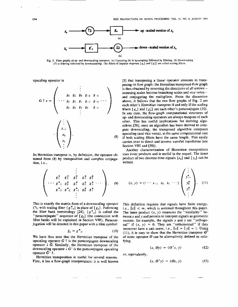
(c) Fig. 4. Flow-graph implementation of the pyramid transform. (a) One step of decomposition; the original signal x is decomposed into a version of x at half its scale, and a residue signal at the same scale and half the resolution, the latter being obtained by difference. (b) The reconstruction part uses (26). One simply adds back what was subtracted before. (c) The elementary cell o f (a) and (b) is iterated J times to provide a full pyramidal decomposition on J “octaves” (here J = 3) .

image coding purposes; here we describe pyramid decom- positions for one-dimensional signals in the framework of this paper. A pyramid transform on J “octaves” decomposes the signal {x,} into the collection of residue signals at scale 2-(’-’) and resolution 2-’, where j = 1 , * , J , plus a IOW resolution version of {x,} , namely the scaled signal at scale and resolution 2-’. This description is sufficient to fully describe a pyramid transform.

It is easy to connect this to the original description of Burt and Adelson [3], by deriving a computational tree- structure for its implementation: Start with one step of decomposition, i.e., let J = 1. From the above definition, the original signal x is decomposed into two components: its residue signal at scale 1 and resolution 1/2, which, from (20), (26) is

plus its scaled version at scale and resolution 1 /2, i.e., 1 G’x. The corresponding flow graph is depicted in Fig. 4(a). To reconstruct x, 1 G‘x is brought back to scale 1 and (26) is applied, i.e.,

G t (1 G’x) + (X - G t l G’x) = X. (29)

In other words, one simply adds what has been previously subtracted. The corresponding flow graph is depicted in Fig. 4(b). This decomposition readily extends to a full computation of a pyramid transform on J octaves. Simply note that from the definition of general multiresolution decomposition, scale and resolution parameters of multiresolution residue signals are halved at each stage (octave) of the decomposition. Now, since any residue signal is a difference of scaled versions of x, the rules (18), (19) ap- ply for residue signals as well. Therefore, scale and resolution parameters of a multiresolution residue signal are halved when replacing x by 1 G ‘ x. This amounts to iter- ating the basic computational structure (one-step decomposition) of Fig. 4 on (1 G ’ ) j x at each level j = 0, - , J - 1 . This gives the flow graph of Fig. 4(c).

In Burt and Adelson’s terminology [3], the above multiresolution residue signals form a Laplacian pyramid, while the set of versions of {x,} at scales 2-’(i = 0, * , J) is called a Gaussian pyramid. The terminology “pyramid” comes from the fact that muiltiresolution components are computed at successive scales, from scale 1 (“base” of pyramid) to scale 2-”- ’) (“top” of pyramid). “Gaussian” and “Laplacian” were named after the type of scaling filters used in [3].

I I


Recall that one always has perfect reconstruction since what has been subtracted is added back during synthesis (see (29)). Therefore, there is no constraint at all on scaling filters { g,} and { g ; }. Even the basic biorthogonality constraint (23), which ensures uniqueness of scaled versions of x at a given scale, is not necessary for the scheme to work. There is a price to pay, however: the multiresolution residue signals correspond to scales s = 2-i(i = 0, - * . , J - 1) that are always twice their resolution r

- s /2 . Therefore the transform is overcomplete: starting from an original signal sampled at rate 1 / T , the multiresolution components of a pyramid transform are sampled at rate 1 /T(1 + 1 /2 + 1 /4 + + 2-J) = 2/T. This means that there are about twice as many transform coefficients as original signal samples. (In two dimensions this factor becomes 4 / 3 [l], [8].)

In contrast with the pyramid transform, the discrete wavelet transform, presented below, is not overcomplete (there are as many wavelet coefficients as signal samples) but requires design constraints on scaling filters.

2-’-1 - - -

*

VII. THE DISCRETE WAVELET TRANSFORM AND

PERFECT RECONSTRUCTION FILTER BANKS We have seen in the preceding section that a potential

drawback of the pyramid transform is its overcomplete- ness, due to the fact that the residue signals involved are “overscaled”, i.e., they satisfy s = 2r. In a “discrete wavelet transform (DWT),” each residue signal is “critically sampled,” i.e., its scale and resolution parameters are equal, r = s. To describe the DWT we therefore need to extend the basic definition of residue signals (26) to this case, which violates restriction (27).

We are led to consider two operators, H t and 1 H’, defined similarly as G t and 1 G ‘ , with impulse responses {h,} and { h ; } , respectively. Define 1 H‘x as the residue signal of x at scale 1 /2 and resolution 1 /2 , which is brought back to scale 1 by applying H t; this gives H t l H’x as the residue signal at scale 1 and resolution 1 /2 defined by (28), i.e.,

(30)

‘ x - G t l G‘x = H t l H ‘ x .

This condition is simply a rewriting, in operator notation, of perfect reconstruction (without delay) of a two-band filter bank [23] depicted in Fig. 5(a), with low-pass filters { g,}, { g ; } and high-pass filters { h,} , {h;} . This definition of residue signals at scale and resolution r = s = 1/2 is immediately extended to other values of r = s by application of the rules (18), (19) as in the preceding section. This gives 1 H ’ ( 1 G’)’- ‘x as the residue signal at scale and resolution r = s = 2 - J ( j > 0).

Using this extended definition of multiresolution residue signals, a DWT on J “octaves” is simply defined as the transformation of a signal {x,} into the following “wavelet coefficients” {wi}, j = 1 , 1 , J , which are precisely the residue signals 1 H’ ( 1 G ’ )’- ’x at scale and resolution r = s = 2-J, and a low resolution signal, { U : ) , the scaled version of x at scale and resolution 2-’.

To reconstruct {x,}, residue signals are first upscaled by means of H t (as in (30)), then definition (26) is applied iteratively to increase resolution until resolution 1 is reached, i.e., until the original signal (x,} is recovered. This is performed by the “inverse DWT” (IDWT).

The DWT and the IDWT are easily recognized to be an octave-band filter bank [23]: To halve both resolution and scale of residue signals, x is replaced by 1 G’x according to rule (18), i.e., the two-band filter bank of Fig. 5(a) is applied to the scaled version ( 1 G’)’x at each levelj. This gives the flow graph of Fig. 5(b), where the analysis filter bank computes the DWT, whereas the synthesis filter bank computes the IDWT. Note that this filter bank is critically sampled, i.e., there are as many computed wavelet coefficients as signal samples, as opposed to the pyramid transform, which is overcomplete by 50% (Section VI). However, low-pass ({ g,} , { g L}) and high-pass ({ h,} , {h;}) filters are constrained to satisfy the perfect reconstruction property (30).

Although the computational structures of the DWT and octave-band perfect reconstruction filter bank are identi- cal, the DWT provides an alternative formalism, which describes it as a multiresolution decomposition in time, rather than as a subband frequency decomposition. This formalism can be developed by defining “basis functions” onto which the signal is decomposed: The basic analysis (synthesis) “scaling sequence” is g ; (g,, respectively), while the basic analysis (synthesis) “wavelet” is the corresponding high pass impulse response & (h,, respectively). Other scaling sequences and wavelets are obtained from the “basic” ones by successive up- scalings:

Analysis scaling sequences:

g’J = (GI t ) J - ’ g ’ . (31)

L‘J = (e’ t )J - IL’. Analysis wavelets:

(32)

Synthesis scaling sequences:

gJ = (G t ) J - lg . (33)

hJ = (G t ) ’ - ’h . (34)

Synthesis wavelets:

Appendix C shows that the wavelet coefficients w/k of the original signal {x,} at oc tave j ( j = 1, - - , J), i.e., the residue signal at scale and resolution 2-’, are inner products of {x,} with the corresponding analysis wavelets:

wJk = (x,, / i ; J - . 2 J k ) , j = I , - 9 J . (35)

(36)

Similarly the low resolution component is J

U : = (xn, g A - 2 J k ) .

An alternative definition of the DWT is thus (35), (36). The inverse DWT reconstructs the signal as a linear combination of shifted synthesis wavelets weighted by the corresponding wavelet coefficients, plus a very low res-

I I


-4 residue: scale=resolution= 1 / 2 residue: scale=resolruion= 114 residue: scale=resolution= 1 / 8

-,,; scaled version: scale=rcsolution= 1/8

4 w.’

3 W”

4 (b)

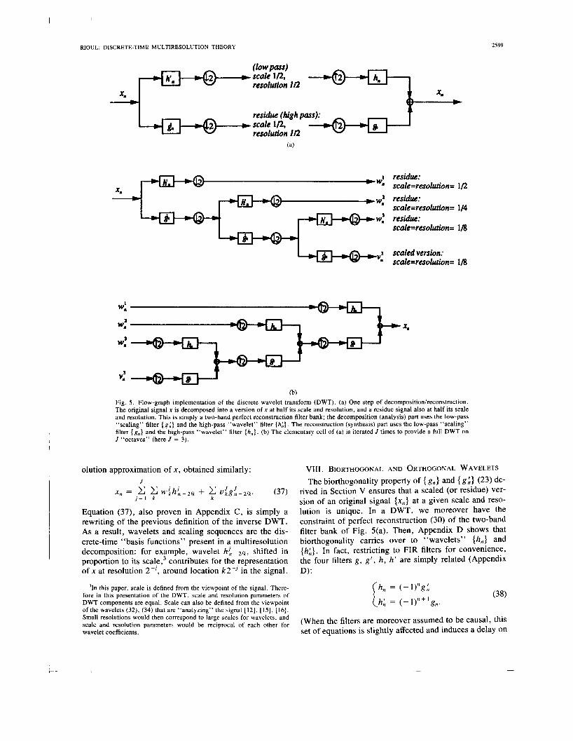
Fig. 5. Flow-graph implementation of the discrete wavelet transform (DWT). (a) One step of decomposition/reconstruction. The original signal x is decomposed into a version of x at half its scale and resolution, and a residue signal also at half its scale and resolution. This is simply a two-band perfect reconstruction filter bank; the decomposition (analysis) part uses the low-pass “scaling” filter { g:} and the high-pass “wavelet” filter { h : } . The reconstruction (synthesis) part uses the low-pass “scaling” filter { g n } and the high-pass “wavelet” filter { h ” } . (b) The elementary cell of (a) is iterated J times to provide a full DWT on J “octaves” (here J = 3).

I

olution approximation of x, obtained similarly:

Equation (37), also proven in Appendix C, is simply a rewriting of the previous definition of the inverse DWT. As a result, wavelets and scaling sequences are the discrete-time ‘‘basis functions” present in a multiresolution decomposition: for example, wavelet hJ, - p k , shifted in proportion to its scale,3 contributes for the representation of x at resolution 2-J , around location k2-’ in the signal.

’In this paper, scale is defined from the viewpoint of the signal. There- fore in this presentation of the DWT, scale and resolution parameters of DWT components are equal. Scale can also be defined from the viewpoint of the wavelets (32), (34) that are “analyzing” the signal [12], [15], [16]. Small resolutions would then correspond to large scales for wavelets, and scale and resolution parameters would be reciprocal of each other for wavelet coefficients.

VIII. BIORTHOGONAL AND ORTHOGONAL WAVELETS The biorthogonality property of { g,} and { g;} (23) de-

rived in Section V ensures that a scaled (or residue) version of an original signal {x,} at a given scale and resolution is unique. In a DWT, we moreover have the constraint of perfect reconstruction (30) of the two-band filter bank of Fig. 5(a). Then, Appendix D shows that biorthogonality carries over to “wavelets” {h , ) and {h ; } . In fact, restricting to FIR filters for convenience, the four filters g, g ’ , h, h’ are simply related (Appendix D) :

h, = (- l)”gi

h; = ( - 1)” + ’ g,.

(When the filters are moreover assumed to be causal, this set of equations is slightly affected and induces a delay on

2600 IEEE TRANSACTIONS ON SIGNAL PROCESSING, VOL. 41. NO. 8, AUGUST 1993

the output of the filter bank.) To design a DWT, it is therefore sufficient to find two low-pass filters satisfying biorthogonality (23) and to define high-pass filters by (38). In addition, the two families of analysis and synthesis wavelets are mutually biorthogonal not only across time shifts at a given scale, but also across scales:

1 i fk = l and i = j (39) i 0 otherwise.

(hi - 2jk, fi;!- 2‘1) =

A proof is given in Appendix D. In fact Appendix D shows that biorthogonality is already implied by perfect reconstruction, and therefore always occurs in a DWT.

Biorthogonality of wavelets (39) is perhaps easier to understand if we note that, in (37), the term contributing to resolution 2-’ is

Now (39) implies that (40) is a projection of x onto the subspace of signals spanned by the wavelets since if x belongs to this subspace, then using (39) one finds that (40) reduces to x . In other words, owing to biorthogonality , the DWT decomposes a signal into pro- jections of this signal onto subspaces corresponding to different resolutions 2-’ ( j = 1 , , J). This point of view is the discrete counterpart of the original theory of Mallat [15], [16] and Meyer [17].

The Orthonormal Case We have seen in Section VI that the orthonormal case

is a special case of biorthogonality for which one further imposes (24), i.e., g , = g ; . From (38) this implies h, = fi;; analysis and synthesis wavelets are equal. From the discussion of Section IV, it follows that the analysis and synthesis filter banks of Fig. 5(b), which, respectively, perform the DWT and IDWT, are Hermitian transpose of each other. In other words the DWT is an orthogonal transform: it is composed of lossless or paraunitary two- band filter banks [24] for which analysis and synthesis filters are paraconjugate of each other. The orthogonal discrete wavelet transform was first connected to the pyramid transform, in a similar manner as in Section VII, by Adelson et al. [l].

From (39) and the relation h, = f i ; , the wavelets form an orthonormal basis:

1 i f k = I and i = j (41)

hence (40) is now an orthogonal projection of x . This means that among all signals y belonging to the subspace spanned by the {hi-2Jk}, (40) is the one that minimizes the quadratic distance 1Ix - y(I2 . Therefore, orthonormality can also be thought of as the condition under which multiresolution components are most similar to the original signal [ 151.

Orthonormality is often considered as an essential property for coding applications (see, e.g., [15]), where

i 0 otherwise (hi-zk, hk-w) =

the coding strategy is based on an LMS error criterion. It also simplifies the design: scaling and wavelet sequences are simply related since (38) reduces to h, = (- 1)”g:- , - n for causal filters. However, it is well known [8], [91, [23], [26] that orthonormal filters cannot be of linear phase, except for a trivial choice; this has motivated the search for biorthogonal, linear phase wavelets r41, ~ 1 .

IX. COMPARISON WITH WAVELET SERIES There is a remarkable parallelism between the DWT,

presented in the previous section, and its continuous-time counterpart, which has been developed for functions of a continuous variable by Meyer [17], Mallat [15], [16], Daubechies [8] and other authors. We refer to the latter as the “wavelet series decomposition” (see (3) and (4)). This section compares the two models within the framework of this paper. The relationship of discrete and continuous wavelet transforms was also clarified by Shensa 1221.

The analog model uses a continuous version of the inner product, namely,

( x ( t ) , Y W ) = 1 x ( t ) Y * ( t ) dt (42)

and applies to analog signals x ( t ) of finite energy I l ~ ( t )11~ = ( ~ ( t ) , x ( t ) ) . Also, upscaling is the simple dilation x ( t )

+ x ( t / 2 ) / & . (In the presentation of the DWT above, the constant h has been integrated into the discrete scaling sequences.) As in the DWT, one defines analysis and synthesis basic scaling functions, denoted by +(t) and cp (t), respectively, and analysis and synthesis basic wavelets $ (t) and $ (t). The whole set of scaling functions and wavelets is defined as in (31)-(34) by successive upscalings. For example, the synthesis wavelets are $’(t) = 2-’12 $(2-’t), and the other basis functions involved, namely, cp’(t), $’( t ) , and +’(t) are defined similarly. Then, the wavelet series coefficients are (compare with (3% (36))

wi, = ( x ( t ) , $’(l - 2jk))

V i = ( ~ ( t ) , G J ( t - 2 J k ) ) (43)

and the reconstruction part uses a wavelet series (compare with (37))

J

x ( t ) = ,x c Wi,$’(t - 2’k) + VicpJ(t - 2Jk). j = I k

(44)

Analog wavelets are biorthogonal (compare with (39))

( $ ’ ( t - 2 ’ k ) , $ i ( t - 2‘1))

1 i f k = 1 a n d i = j (45) =i 0 otherwise

and, of course, orthonormality occurs when analysis and synthesis wavelets are equal. Other properties, such as

I I


phase linearity [4], [26] and finite or “compact” support [4], [8], [26], are also expressed similarly as in the discrete-time case.

Therefore, the sole ability of the wavelet transform to do multiresolution signal decomposition, using orthonormal or biorthogonal bases, should not be critical in decid- ing whether to choose the discrete-time model or the continuous-time one, because both models share the same properties. In fact, the parallelism that exists between the discrete-time and the continuous-time formalisms is so strong that a DWT can always be deduced from a biorthogonal analog wavelet basis [4]. Specifically, discrete and continuous-time “basis functions” are related by [4]

+(t) = Jz c g;+(2t - n) n

$(t) = Jz c &+(2t - n) n

cp(t) = Jz c g,cp(2t - n )

$(t) = h hncp(2t - n ) . (46)

n

n

Furthermore, additional properties satisfied by continuous-time wavelets, such as orthonormality , symmetry, and finite support are automatically fulfilled by the associated discrete-time wavelets [4], [8]. Thus, a continuous wavelet series decomposition scheme induces an associated DWT, the latter being implemented as an octave-band filter bank. Moreover, fed by the discrete input { V : } , this filter bank provides the continuous-time wavelet series coefficients { W i } ( j = 1, * - * , J ) and { V i } [4]. The algorithm was first derived by Mallat [15] in the context of orthonormal wavelets and was generalized for other types of continuous wavelets transforms by Shensa [22].

However, any arbitrary DWT cannot always be deduced from a wavelet series decomposition scheme, because this would imply that the obtained discrete wavelets satisfy constraints other than biorthogonality . For example, they would satisfy the relations [4] C,h, = E,& = 0, which are not always met in perfect reconstruction filter banks (see [23]).

This has motivated several researchers to determine the minimal conditions under which continuous-time wavelet bases can be deduced from discrete-time ones. Necessary and sufficient conditions were recently derived, which turned out to be quite technical [4], [14]. It was previously shown [SI, however, that a sufficient condition for the equivalence between the continuous-time case and the discrete-time case is the regularity property, which is by itself interesting; it is discussed in the next section.

X. FILTER REGULARITY Regularity is well understood for continuous-time

wavelets; they are regular if they are at least continuous, possibly with several continuous derivatives. Evidently this cannot be expressed directly on discrete-time signals, and the regularity property seems to be an exception to the rule that the discrete-time and continuous-time models

share the same properties. Nevertheless, the aim of this section is to show that regularity can be defined for discrete-time wavelets, and that the two definitions of regularity are in fact equivalent.

Regularity, introduced by wavelet theory as a smoothness condition on continuous-time wavelet basis functions, was soon recognized as a new design constraint for perfect reconstruction filter banks which is used to construct regular continuous-time wavelets [4], [8], [26]. Therefore, we want to characterize this constraint as a smoothness condition on the discrete-time ‘‘basis functions” defined in Section VII. These “basis sequences” are obtained by successive up-scalings: the aim is to find the conditions on the upscaling operator G t (6) under which signals (G t)’x vary smoothly, even for large j . We then say that the underlying scaling filter { g,,} is “regular.”

In a biorthogonal DWT, for example, regularity of the scaling filter { g,,} implies regularity for all synthesis discrete wavelets and scaling sequences, since they are defined by successive up-scalings associated to { g,} (33), (34). On the other hand, regularity of analysis discrete wavelets and scaling sequences (31), (32) holds if the scaling filter { g;} is regular. Note that regularity can also be studied for pyramid transforms because their equivalent basis functions are also of the form (G t)’x, and in fact regularity was first observed by Burt and Adelson [3] in the framework of pyramidal decomposition.

Regularity is believed to be useful in multiresolution decomposition schemes for several reasons [ 181, [2 11. In a DWT, for example, any error occurring in a wavelet coefficient w$ results, from (37), in a perturbation in the synthesized signal which is equal to the corresponding synthesis wavelet sequence { h i - 2 , k ) . It is therefore nat- ural to require that this perturbation be smooth, rather than discontinuous, or even fractal, as in the example shown in Fig. 6(a). This may be useful in, e.g., image coding applications where a “fractal” perturbation is likely to “strike the eye” much more than a smooth one, for the same SNR level [2]. On the other hand, requiring that the signal be analyzed by smooth basis functions {LA’} ensures that no “artificial” discontinuity (i.e., not due to the signal itself) appears in the wavelet coefficients w/k = (x,,, LA’- 2 , k ) . This should also be of interest for compression purposes [2], [27].

A . De$nition of Regularity We now define regularity for discrete-time signals

(G t)’x, i.e., for responses to the operator (G t)’, restricting to the impulse responses gJn = ((G t )’@,, for convenience. The following definition of regularity is inspired from Holder regularity of continuous-time functions [ l l ] , [19]: For 0 < a 5 1, g i is said to be regular of order r = (Y if it satisfies

(47)

where c is the constant independent of j and n. In other

26M IEEE TRANSACTIONS ON SIGNAL PROCESSING, VOL. 41, NO. 8, AUGUST 1993

words, the slopes

A g i = (g’,+1 - g’,>/2-’ (48)

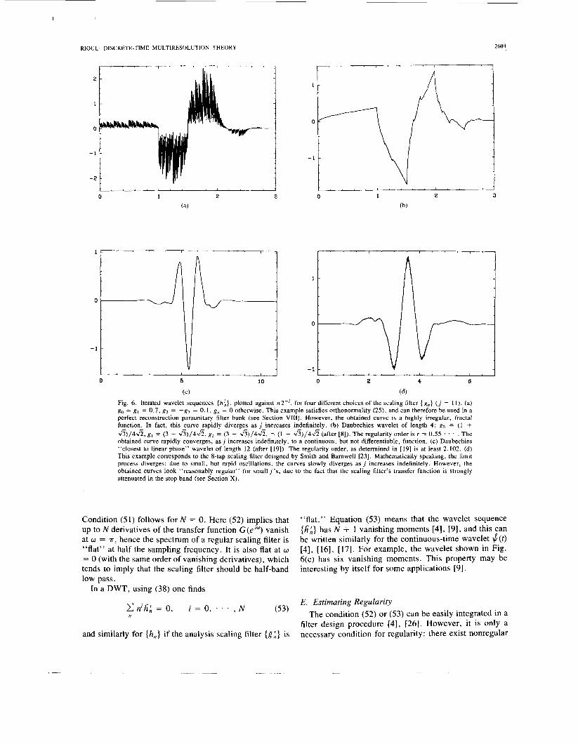
of the curve g’, plotted against n2-’, are constrained to increase less than 2’(’-@ as j increases: for a < 1 they may indefinitely increase (Fig. 6(b) shows an example which satisfies (47) for a = 0.550 [8], [9], [ l l ] ) ; for CY = 1 they are always bounded (see Fig. 6(c)). Of course, the regularity condition (47) is stronger as a increases, thereby imposing smoother time evolutions of the sequence { g i } .

In order to extend this definition to higher regularity orders, we impose (47) on the “discrete derivatives” of g’,. The first “discrete derivative” of g i is the sequence of slopes (48). The Nth discrete derivative ANgi is defined by applying N times the difference operator A. Now, g’, is said to be regular of order r = N + a (0 < a 5 1) if its Nth discrete derivative ANgi is regular of order CY,

i.e., if

-

lANg{+l - ANg’,l S ~ ( 2 ~ ’ ) ” . (49)

The example of Fig. 6(c) is regular of order r > 2.102 [ 191. Again this definition imposes a stronger condition as r increases; here condition (49) is imposed on “slopes of slopes” and therefore requires very smooth evolutions of g i .

B. Connection with Wavelet Series

It can be shown [I91 that regular discrete wavelet and scaling sequences converge toward continuous-time functions as j -+ 03. More precisely, the discrete curves { gi}, { g:’}, { h i } and {LA’}, when plotted aBainst n2-j, uniformly converge to p ( t ) , + ( t ) , II/ ( t ) , and II/ ( t ) , respectively. In addition, these limit functions have the same Holder regularity order r as their discrete counterparts [19], Holder regularity r = N + CY (0 < QI 5 1) for the continuous-time case being defined similarly as

((p“’(t + h) - (p(”(t)l 5 c(h(” (50)

where ~ ( ~ ’ ( t ) is the Nth derivative of p ( t ) (compare with (49)). Note that a Holder regularity order r > N implies N continuous derivatives.

Now, the continuous-time limits 8 ( t ) , + ( t ) , $ ( t ) , and (t) can be used to define a wavelet series decomposition

as in Section IX. Compactly supported continuous-time wavelets have been designed by this method [4], [8], [9]. Therefore, owing to regularity, the identification between discrete-time and continuous-time wavelet schemes is complete: it is only a matter of opinion to state that continuous-time wavelets underlie discrete-time ones (from (46)) or vice versa (from the limit process). Likewise, the regularity property can be seen either on continuous-time functions (50) or on discrete-time sequences (49).

C. A First Necessary Condition for Regularity

I

Regularity of the scaling filter { g,} also implies shape preservation by the upscaling operator G t (this is As-

sumption 3) of Section 111). In other words, upscaling “stretches” the sequence {g’,} but does not affect its shape: we have g!, = gin+ I z gin+: ,, the approximations being sharper as j increases. Now since gJ + ’ = G t g’, using (6), we have gin+ = Ckg2kg i -k = (Ckg2Jgi, hence &gSk = 1. Similarly it can be shown that CkgZk+ I = 1, starting from g<nf: I ([ 191 contains a more rigorous proof). These conditions are necessary conditions for shape preservation and regularity. They can be rewritten as C,g, = 2 and E,(- l ) ”g, = 0, i.e.,

2 i f w = O

0 i f w = ? r G(eJ“) =

where G(e’”) is the transfer function of the scaling filter of impulse response { g,} . This justifies that scaling filters are preferably low pass. In fact, they are often chosen to be half-band low-pass filters, a property that is justified by stronger regularity conditions (see below). Note that the first condition in (51) is simply a renormalization: In an orthogonal DWT, for example, they are normalized such that [8] C,g, = C,gL = h so that orthogonality (25) holds. Hence, the order of magnitude of {g i } de- creases as 2-J” as j increases, and one has to renormalize { g,} according to (51) so that the order of magnitude of { g!,} is preserved for different j ’s.

Fig. 6 shows several examples of iterated wavelet sequences { h i } corresponding ,to different choices of { gn} . In Fig. 6(a), the curve { h i } rapidly diverges as j increases. This example does not even fulfill (51), therefore it is not continuous. The example shown in Fig. 6(b) is the first Daubechies wavelet of length 4 [8]. It satisfies (51) but is clearly not very regular; this shows that (51) is not sufficient to obtain a high regularity order. Fig. 6(c) is a very regular example (see below). The example of Fig. 6(d) is particularly interesting: it corresponds to one of Smith and Bamwell filters derived in [23]. Mathemat- ically speaking, this example is not regular because (51) is not satisfied. However, in this case, the scaling filter has a 40-dB attenuation in the stopband, and the value of G(e’“) at w = ?r is thus very small (about As a result, (51) is “almost” satisfied and the iterated sequences { h i } “pretend” to be regular for small j ’ s . For large j ’ s the curves eventually diverge, with strong oscil- lations near the wavelet modes (see Fig. 6(d)). Although rejected by the mathematical definition above, such wavelets may be “regular enough” in applications where the number of octaves in the multiresolution decomposition is not too large.

D. Necessary Conditions for Regularity: “Flat Filters ’’ or “Vanishing Moments”

A regularity order r > N requires more than (51). In fact it can be shown [4], [19] that the scaling transfer function G(e’”) is necessarily of the form

N + I

(52) G(e’”) = (7) 1 + e-’“ F(e’“).

I I

0

- 1

RIOUL: DISCRETE-TIME MULTIRESOLUTION THEORY

1 - ’ ’ ’ “ ’ . ’ I 3

1 -

0

-

-1 - , . . . I . . . , .

2603

0 3

Condition (51) follows for N = 0. Here (52) implies that up to N derivatives of the transfer function G(e’”) vanish at w = T , hence the spectrum of a regular scaling filter is “flat” at half the sampling frequency. It is also flat at w = 0 (with the same order of vanishing derivatives), which tends to imply that the scaling filter should be half-band low pass.

In a DWT, using (38) one finds

and similarly for {h , } if the analysis scaling filter { g ; } is

“flat.” Equation (53) means that the wavelet sequence (6 ; ) has N + 1 vanishing moments [4], [9], and this can be written similarly for the continuous-time wavelet IJ (t) [4], [16], [17]. For example, the wavelet shown in Fig. 6(c) has six vanishing moments. This property may be interesting by itself for some applications [9].

E. Estimating Regularity The condition (52) or (53) can be easily integrated in a

filter design procedure [4], [26]. However, it is only a necessary condition for regularity: there exist nonregular


examples for which (52) holds [19]. It is therefore important to a posteriori determine the regularity order of a computed scaling filter { g,} , and several regularity estimates have been derived for the purpose [8], [ 113. Dau- bechies’ estimate [8] is based on the determination of maxima of spectra. Unfortunately, it requires many com- putations to determine a good estimate and is not optimal in general [ 191. Daubechies and Lagarias [lo], [ 1 11 have derived a method based on matrix algebra which yields optimal regularity estimates in some instances. The author derived a method in [19], which, unlike earlier estimates, is based on the discrete-time approach described in this section. It is easily implementable, applicable in all cases, and gives optimal estimates for Holder regularity.

XI. CONCLUSION This paper has developed an alternative view of mul-

tiresolution theory which focuses on discrete-time signals. It is based on precise notions of scale and resolution in discrete-time (Sections 111 and V). We have described both the pyramid transform (Section VI) and the discrete wavelet transform (Sections VI1 and VIII) using these notions. Pyramid transforms uses “overscaled” multiresolution components, while scale and resolution parameters of DWT coefficients are equal.

Biorthogonality is derived as an essential condition for scaled versions of an original signal to be characterized by scale and resolution parameters (Section V). In a DWT, it is also implied by the perfect reconstruction property (Section VIII). Orthonormality is a special case of biorthogonality, in which DWT and inverse DWT flow graphs are self transposed.

The discrete-time multiresolution theory derived here shares the same properties as the continuous-time multiresolution theory of Mallat [15], [16] and Meyer [17]. These properties include basis expansion, scale and resolution notions, orthogonality or biorthogonality , and regularity. Therefore, it is only a matter of taste to decide whether analog wavelets underly discrete-time ones or vice versa. The DWT provides a coherent alternative, which has advantages and drawbacks. For example, a change of scale is evidently not so easily expressed for discrete sequences that it is for continuous-time signals. The discrete approach, however, avoids technical proofs or makes them easier and readily provides numerical algorithms. Of course, discrete-time multiresolution theory also gives a new way of looking at filter banks; it describes them as a temporal multiresolution decomposition rather than as a subband frequency decomposition.

New criteria in filter design are also brought by wavelets. In particular, there is a, presumably important, notion of regularity. In Section X we have briefly discussed the regularity property in the framework of discrete-time wavelets. Although regular filters have been used in practical systems [2], [15] it is still not clear whether regularity is to play an important role in applications such as image coding.

APPENDIX A GENERAL EXPRESSIONS FOR SCALING OPERATORS

Proof of (6): Let { g,} be the impulse response of the upscaling operator, that is, the upscaled version of the pulse signal 6,. By assumption 2), g n - 2 k is the response to 6, - k . Since the input signal can be written

x , = c x k 6 , - k

its upscaled version is, using linearity l ) ,

X k g n - 2k

U which is (6). Proof of (7): Let { g:} be the impulse response of

the downscaling operator to {A,}, and { g! - I } be the impulse response to { 6, - The input signal can be written

x , = T X 2 k s n - 2 1 1 + X 2 k + 1 6 n - I - 2 k .

Its downscaled version is therefore

k

Now let { g ; } be defined by g;, = g: and g;,+l = g!. The downscaled version becomes

C X 2 k g ; n - 2 k k + X 2 k + l g ; n - 2 k - l

0 which reduces to (7).

APPENDIX B DERIVATION OF BIORTHOGONALITY

From any possible expression of upscaled versions of { x , } , simplify using (21) each time this is possible to obtain a unique expression for a version of { x , } at a given scale 2-’ and resolution 2-j(j 2 i ) , namely, (G t)’-‘( 1 G ’ ) J x . Condition (21) is therefore sufficient for uniqueness of a version of x at a given scale and resolution. In addition, since A approximates at half the resolution, it should leave Ax itself unchanged. That is, both Ax and A2x are at scale 1 and resolution 1 /2, so they are equal and (22) is a necessary condition for uniqueness. We have seen in Section V that (21) implies (22). There- fore, if we show the converse implication, then both conditions (21) and (22) will be equivalent to uniqueness.

Proof of (22) * (21): Equation (22) can be written, using (20), G t y = 0, where y = 1 G ’ ( G t l G ’ - Z ) x . Now since upscaling is one to one (17), this yields y = 0, i.e.,

(1 G ‘ G t -Z ) 1 G ’ x = 0

for all signals x . We now prove that any signal y with finite energy can be written 1 G ’ x for some x . We can always write y = y ’ + y ”, where y ’ belongs to the range of the downscaling operator 1 G (hence it can be put in the form 1 G ’ x for some x ) , and where y ” is orthogonal to any signal of this range:

( y ” , 1 G ‘ z ) = 0 for all signals z .

I


Using the transposition property (15) one obtains

(6’ ? y ” , z ) = o for all z hence 6’ t y “ = 0, which implies y ” = 0 similarly as for G t (17). Therefore any signal y can be written y = y ’ = 1 G’x for some x. Now from the equation (1 G ’ G t - I ) 1 G‘x = 0, (21) immediately follows. 0

This shows that uniqueness is equivalent to (21) and to (22). We now show that biorthogonality is also equivalent to (21).

Proof: Using the transposition property (15) and the relation

1 i f k = l i 0 otherwise ( 6 n - k , 6 n - / ) =

we have

( g n - 2 k 9 g A - 2 1 ) = ( ( G t a ) n - 2 k , (6’ t 6)n-2/)

= ( ( G t (6’ t 6 n - I ) )

= ((4 G ‘ G t 6 n - k ) , 6 n - / )

- - (6n-k , A n - / )

1 i f k = l = i 0 otherwise

which shows that (23) and (21) are equivalent.

APPENDIX C DISCRETE WAVELET BASES

Proof of (35) and (36): The residue signal at resolution and scale 2’ can be written

wjk = (1 H ’ ( 1 G ’ ) j - ’ X ) k

= ((1 H ’ ( 1 G ’ ) j - ’ x n , an- , ) .

Using the transposition property (15) we have

= ( x n , ((6’ ? ) f p ’ P ) n - 2 ] k )

which reduces to (35) by definition of &” (32). One proves similarly that v J = (1 G ’ ) ’ x reduces to (36).

Proof of (37): To reconstruct the signal, the wavelet coefficients w J , and uJ are brought back to scale 1 and (26) is applied. This gives

J

x = c (G t)’-’H t wj + (G ? ) J U J .

Using the formula w’, = C k wjk6, - k (and similarly for U J ) , linearity and (33), (34), this equation is easily seen to reduce to (37). o

j = 1

APPENDIX D PERFECT RECONSTRUCTION AND BIORTHOGONALITY

Proof of (38) and Biorthogonality (39), Assuming Perfect Reconstruction (30): It is well known [23], [24] that perfect reconstruction of the filter bank of Fig. 5(a)

can be written as two conditions on z transforms of filters, namely,

(D1)

(D2)

Assuming (noncausal) FIR filters, z transforms are poly- nomials in z and z - ’ . Now, consider four polynomial fac- tors of low-pass filters, defined by G(z ) = GH(z)GH,(z) and G ’ ( z ) = GA(z)GA.(z), which satisfy, from (D2), H ( z ) = GH(z)GA(-z) and H ‘ ( z ) = -GH,(-z)Gk,(z) . Consequently, a common factor of (Dl) is GH(z)Gk,(z); both terms divides a constant polynomial, and can therefore be chosen equal to one, GH(z) = GA,(z) = 1. We therefore end up with H ( z ) = G ’ ( - z ) and H ’ ( z ) = -G( - z ) , which is (38), and perfect reconstruction reduces to

G(z )G’ ( z ) + H ( z ) H ’ ( z ) = 2 i G ( z ) G ‘ ( - z ) + H ( z ) H ’ ( - z ) = 0.

G(z )G’ ( z ) - G ( - z ) G ’ ( - z ) = 2

which is (23). We have seen in Section V that (23) is equivalent to

1 G’ G t = I . From the relations (38) one similarly proves that 1 H’H t = I. Now, using definitions (32) and (34), and the transposition property (15), the left-hand side of (39) can be written

((G t ) ’ - ’ H t (6’ ? ) ’ - ‘ f i r t a n - / ) = (1 H ’ ( L G’)’-I(G T ) ’ - ’ H t 6 , - k , A n - / )

which reduces to the right-hand side of (39). 0

ACKNOWLEDGMENT The author would like to express his appreciation to I.

Daubechies of Rutgers University, A. Grossmann of the University of Marseilles-Luminy, and Y. Meyer of Paris- Dauphine University, for introducing him to mathematical aspects of wavelets when it was very new. He is also grateful to M. Vetterli and C. Herley of Columbia Uni- versity, New York, for valuable discussions on filter banks, pyramids, and wavelets. Finally, he thanks P. Du- hamel of CNET, Paris, for carefully reading the manuscript, and the anonymous reviewers for their valuable feedback.

REFERENCES

[ I ] E. H . Adelson, E. Simoncelli, and R. Hingorani, “Orthogonal pyramid transforms for image coding,” Proc. SPIE Int. Soc. Opt. Eng. , vol. 845, pp. 50-58, Oct. 1987.

[2] M. Antonini, M. Barlaud, P. Mathieu, and I . Daubechies, “Image coding using vector quantization in the wavelet transform domain,” in Proc. 1990 IEEE Int. Conf. Acoust., Speech, Signal Processing, Albuquerque, NM, Apr. 3-6, 1990, pp. 2297-2300.

[3] P. J . Burt and E. H. Adelson, “The Laplacian pyramid as a compact image code,” IEEE Trans. Commun., vol. COM-31, no. 4 , Apr. 1983.

[4] A. Cohen, I . Daubechies, and J . C . Feauveau, “Biorthogonal bases of compactly supported wavelets,” Commun. Pure Appl. Math., to be published.

[SI R. E. Crochiere and A . V . Oppenheim, “Analysis of linear digital networks,” Proc. IEEE, vol. 63, pp. 581-595, Apr. 1975.

[6] R. E. Crochiere and L. R. Rabiner, Multirate Digital Signal Pro- cessing. Englewood Cliffs, NJ: Prentice-Hall, 1983.


[7] R. E. Crochiere, S . A. Weber, and J . L. Flanagan, “Digital coding of speech in subbands,” Bell Syst. Tech. J . , vol. 55, pp. 1069-1085. Oct. 1976.

[8] I. Daubechies, “Orthonormal bases of compactly supported wavelets,” Commun. Pure Appl. Math., vol. 41, no. 7, pp. 909-996, 1988.

191 I . Daubechies, ‘‘Orthonormal bases of compactly supported wavelets, 11. Variations on a theme,” SIAM J . Math. Anal. , to be published.

[IO] I. Daubechies and J. C . Lagarias, “Two-scale difference equations, I . Existence and global regularity of solutions,” SIAM J . Math. Anal. , vol. 22, no. 5 , pp, 1338-1410. Sept. 1991.

[ I 11 I. Daubechies and J . C . Lagarias, “Two-scale difference equations, 11. Local regularity, infinite products of matrices and fractals.” SIAM J . Math. Anal . , to be published.

[12] P. Goupillaud, A. Grossmann, and J. Morlet, “Cycle-octave and related transforms in seismic signal analysis,” Geoexploration, vol. 23, pp. 85-102, 198411985,

[ 131 0. Henmann, “On the approximation problem in nonrecursive digital filter design,” IEEE Trans. Circuit Theory, vol. CT-18, no. 3, pp. 411-413, May 1971.

[I41 W. M. Lawton, “Necessary and sufficient conditions for constructing orthonormal wavelet bases,” Aware, Rep. AD900402, Cambridge, MA, 1990.

1151 S. Mallat, “A theory for multiresolution signal decomposition: The wavelet remesentation.” IEEE Trans. Putt. Anal. Machine Intell..

(191

1201

- . vol. 11, no. 7, pp. 674-693, July 1989. S . Mallat, “Multiresolution approximations and wavelet orthonormal bases of L2(R) ,” Trans. Amer. Math. Soc . , vol. 315, no. 1 , pp. 69-87, Sept. 1989. Y. Meyer. Ondelettes et OpPrateurs, Tome I. Paris: Henmann, 1990. 0. Rioul, “Simple, optimal regularity estimates for wavelets,” in Proc. 6th Eur. Signal Processing Conf. (EUSIPCO’92). Brussels, Belgium, August 24-27, 1992. 0. Rioul, “Simple regularity criteria for subdivision schemes,” SIAM J . Math. Anal . , vol. 23, no. 6, pp. 1544-1576, Nov. 1992. 0. Rioul and P. Duhamel, “Fast algorithms for discrete and continuous wavelet transforms,” IEEE Trans. Inform. Theory (Special Is- sue on Wavelet Transforms and Multiresolution Signal Analysis), vol. 38 , no. 2, pp. 569-586, Mar. 1992. 0. Rioul and M. Vetterli, “Wavelets and signal processing.” IEEE Signal Processing M a g . , vol. 8. no. 4 , pp. 14-38, 1991.

1221 M. J. Shensa, “The discrete wavelet transform: Wedding the a trous and Mallat algorithms,” IEEE Trans. Signal Processing, vol. 40, no. 10, pp. 2464-2482, Oct. 1992.

[23j M. J . T . Smith and T. P. Bamwell 111. “Exact reconstruction techniques for tree structured subband coders,” IEEE Trans. Acoust. , Speech, Signal Processing, vol. ASSP-34, no. 3 , pp. 434-441, June 1986.

[24] P. P. Vaidyanathan, “Multirate digital filters, filter banks, polyphase networks, and applications: A Tutorial,” Proc. IEEE, vol. 78, no.

[25] M. Vetterli, “Multidimensional subband coding: Some theory and algorithms,” Signal Processing, vol. 6 , no. 2, pp. 97-1 12, Feb. 1984.

1261 M. Vetterli and C. Herley, “Wavelets and filter banks: Theory and design,” IEEE Trans. Signal Processing, vol. 40, no. 9, pp. 2207- 2232, Sept. 1992.

1271 W . R. Zettler, J. Huffman, and D. C. P. Linden, “Application of compactly supported wavelets to image compression,” Proc. SPIE Int. Soc. Opr. Eng. , vol. 1244, pp. 150-160, Feb. 1990.

1, pp. 56-93, July 1990.

Olivier Rioul was bom in Strasbourg, France, in 1964. He received the Dipl. Ing. degree from the Ecole Polytechnique, Palaiseau, France, in 1987, the Dipl. Ing. Telecom. degree from the Ecole Nationale Superieure des Telecommunications (ENST), Paris, in 1989, and the Doctorat d’ln- g6nieur des Telecommunications (Ph.D.) degree from the ENST, in 1993.

He worked for AT&T Bell Laboratories in 1988. In 1989, he joined the Centre National d’Etudes des Telecommunications (CNET-France

TCICcom) in Issy-Les-Moulineaux, France, where he is currently a Re- search Engineer in the Centre de Recherche en Physique de I’Environne- ment (Unit6 mixte CNRS/CNET). His research interests include wavelets, multirate signal processing, computational complexity, image coding, and signal analysis.

Documents

A discrete-time multiresolution theory - Signal Processing