Embed Size (px)
Citation preview
A Discrete-Continuous Multi-Vehicle Anticipation Model of Driving Behaviour in Heterogeneous Disordered Traffic Conditions
Sangram Krishna Nirmale PhD Candidate
Department of Civil Engineering Indian Institute of Science Bangalore, India, 560012
Email: [email protected] Phone: +91-80-2293-2043
Abdul Rawoof Pinjari (corresponding author) Associate Professor
Department of Civil Engineering Centre for infrastructure, Sustainable Transportation and Urban Planning (CiSTUP)
Indian Institute of Science Bangalore, India, 560012 Email: [email protected]
Phone: +91-80-2293-2043
Anshuman Sharma C.V. Raman Postdoctoral Fellow
Centre for infrastructure, Sustainable Transportation and Urban Planning (CiSTUP) Indian Institute of Science Bangalore, India, 560012
Email: [email protected] Phone: +91-80-2293-2043
February 2021
1
Abstract
This study proposes a multi-vehicle anticipation-based discrete-continuous choice modelling framework for describing driver behaviour in heterogeneous disordered traffic (HDT) conditions. To incorporate multi-vehicle anticipation, the concept of an influence zone around a vehicle (subject vehicle) is introduced. Vehicles within the influence zone can potentially influence the subject vehicle’s driving behaviour. Further, driving decisions are characterized as combination of discrete and continuous components. The discrete component involves the decision to accelerate, decelerate, or maintain constant speed and the continuous component involves the decision of how much to accelerate or decelerate. A copula-based joint modelling framework that allows dependencies between discrete and continuous components is proposed. Such a joint modelling framework recognizes that the discrete and continuous decisions are made simultaneously, and common unobserved factors influence both decisions. Additionally, truncated distributions are employed for the continuous model components to avoid the prediction of unrealistically high acceleration or deceleration values. The parameters of the proposed model are estimated using a trajectory dataset from Chennai, India. The empirical results underscore (a) the importance of considering multi-vehicle anticipation for describing driving behaviour in HDT conditions, and (b) the efficacy of the joint discrete-continuous system for modelling driving behaviour. Further, not all traffic environment variables found to influence the discrete decisions were found influential on continuous decisions and vice versa. Moreover, the influence of several variables was found to be stronger on the decision to accelerate or decelerate than on the decision of how much to accelerate or decelerate.
1. INTRODUCTION
Microscopic traffic flow models describe the driving behaviour at the individual vehicle level by mimicking driver’s decisions to advance in the longitudinal (vehicle-following) and lateral directions (lane-changing) (refer to Brackstone et al. (1999), Toledo (2007), Zheng (2014), Saifuzzaman & Zheng (2014), and Mahapatra et al. (2018) for a detailed review of microscopic traffic flow models). These models are used to perform traffic flow analysis, traffic safety analysis, traffic emission estimation and control studies, build traffic simulation tools, etc. (Brackstone and McDonald, 1999; Gartner et al., 2002; Park and Won, 2006; Toledo, 2007; Saifuzzaman and Zheng, 2014; Ni, 2015; Chakroborty and Das, 2017). A majority of these models are built for homogeneous traffic conditions and cannot be applied to heterogeneous disordered traffic (HDT) where the traffic characteristics are significantly different from the homogeneous traffic conditions (Choudhury and Islam, 2016). HDT conditions may be characterized by the following three features that are not common to homogeneous traffic conditions: (i) a wide variety of vehicles that include motorized two-wheelers, cars, auto-rickshaws, buses, and trucks; (ii) non-lane discipline in vehicular movements; and (iii) a large extent of lateral movements than typically observed in homogeneous traffic conditions (Venkatachalam and Gnanavelu, 2009; Kanagaraj et al., 2015; Asaithambi et al., 2016; Choudhury and Islam, 2016; Munigety and Mathew, 2016; Kanagaraj and

2
Treiber, 2018; Mahapatra et al., 2018; Sarkar et al., 2020). The vehicles have broad differences in shapes, sizes, acceleration-deceleration capabilities, and degrees-of-freedom contributing to the heterogeneity in their microscopic movement characteristics. Moreover, drivers often position themselves in between other vehicles in an attempt to make use of the entire available space, thus occupy multiple lanes. Therefore, microscopic vehicular movements in HDT conditions depict weak to no lane discipline. In summary, the interactions among vehicles and the resulting manoeuvres they undertake are much more complex in HDT conditions (than in homogeneous traffic conditions) necessitating the need for developing dedicated microscopic driving behaviour models for such conditions.
Whether the traffic condition is homogenous or heterogeneous, drivers’ decisions are driven by various factors including human factors, traffic environment, and roadway infrastructure elements. Human factors are often not given their due importance in microscopic traffic flow models which have made them too simple to explain the complex interaction between the human driver and the traffic environment (Sharma et al., 2017). In this context, recent studies have demonstrated the significance of incorporating human factors in the microscopic modelling framework to comprehensively describe the driver’s decision-making process (Saifuzzaman et al., 2015; Sharma et al., 2017; van Lint and Calvert, 2018; Ali et al., 2019; Paschalidis et al., 2019; Sharma et al., 2019; Calvert et al., 2020). One such human factor is multi-vehicle anticipation by the driver. Multi-vehicle anticipation (also known as spatial anticipation) refers to a driver’s ability to take several vehicles around his/her vehicle into account for making his/her driving decisions. Previous studies argue that considering a single lead vehicle as the only influential vehicle may not adequately represent driving behaviour (Bexelius, 1968; Lenz et al., 1999; Hoogendoorn and Ossen, 2006; Hoogendoorn et al., 2006; Treiber et al., 2006; Peng and Sun, 2010; Zhang, 2014). Moreover, multi-vehicle anticipation stabilizes the traffic flow and reduces the destabilizing effect of reaction time (Treiber et al., 2007). Multi-vehicle anticipation is still underexplored in the context of HDT conditions.
The objective of this study is to present a microscopic modelling framework that mimics the driving behaviour in the longitudinal direction in HDT conditions. Importantly, the presented modelling framework incorporates multi-vehicle anticipation by the driver.
The remainder of this paper is structured as follows. Section 2 presents the literature review, research gaps, and positions the contribution of the current study. Section 3 discusses the proposed modelling framework. Section 4 provides an overview of the trajectory dataset, model variables, and their descriptive statistics. Section 5 presents and discusses the model estimation results. Finally, Section 6 summarises the main findings of this study and provides future research directions.

3
2. EARLIER APPROACHES, RESEARCH GAPS, AND THE CURRENT STUDY
2.1. Models for Heterogeneous Disordered Traffic (HDT) Conditions
In the earlier models for HDT conditions, several studies recalibrated the driver behaviour models that are built for homogenous traffic conditions (Hoque, 1994; Hossain and McDonald, 1998; Maini, 2002). Lan and Chang (2004) specifically focused on motorcyclist behaviour and proposed an adaptive neuro-fuzzy inference system (ANFIS) based driver behaviour model. They compared the proposed model with the well-known General Motors car-following model and found that their model performed better. Chakroborty et al. (2004) analysed HDT conditions by proposing a car-following model that considers driver behavior safety and urgency aspects. Mallikarjuna and Rao (2011) aimed to analyze the driving behaviour in mid-block sections of urban and rural roads in the Indian context using a cellular automata approach. Some studies identified the significant effects of the type of vehicle pair (Ravishankar and Mathew, 2011; Choudhury and Islam, 2016) and lead-vehicle size (Maini, 2002; Sayer et al., 2003) in vehicle-following behaviour. Several studies also acknowledged that, in HDT streams, drivers might not strictly follow a single leader, but only be partially aligned with it laterally, following multiple leaders or positioning in between multiple leaders (Cho and Wu, 2004; Gunay, 2007; Lee et al., 2009; S. Jin et al., 2012).
Meanwhile, Choudhury and Islam (2016) used a latent leader approach to model drivers’ decisions in weak lane discipline traffic, assuming that drivers respond to a single lead vehicle that cannot be deterministically ascertained from observation. Therefore, they use the latent class framework to probabilistically identify the lead vehicle. Recently, Munigety (2018) discussed a spring-mass-damper mechanical analogy to model driver-vehicle integrated system for HDT conditions. The proposed single leader spring-mass-damper-based model was extended to consider the effect of multiple surrounding vehicles to model vehicle-following behaviour. Kanagaraj and Treiber (2018) proposed a modified social force model and Sarkar et al. (2020) proposed a two-step multinomial logit plus modified intelligent driver model to describe HDT conditions. Both studies calibrated their proposed model using the vehicular trajectory dataset (Kanagaraj et al., 2015) collected in Chennai, India. A detailed literature review on microscopic models for HDT conditions can be found elsewhere (Asaithambi et al., 2016; Munigety and Mathew, 2016; Das and Maurya, 2018; Mahapatra et al., 2018; Chakroborty et al., 2019).
2.2. Models that Incorporate Multi-Vehicle Anticipation by Driver
Gazis et al. (1959) and Bexelius (1968) are probably the first to have extended the well-known GHR car-following model by incorporating the stimulus from more than one leader. Many researchers have followed a similar line of thought, and different models have been proposed in this context. For instance, Hoogendoorn and Ossen (2006) and Hoogendoorn et al. (2006) extended Helly’s model (Helly, 1959) to consider the impact of multiple lead vehicles and performed empirical analysis on real traffic trajectory data. Zhang (2014) also empirically investigated the multi-vehicle anticipation car-following behaviour using multiple linear regression, whereas the support vector regression approach was utilised by Lu et al. (2015). In a
4
separate study, Tao et al. (2015) improved the GM car-following model to consider the impact of lateral offset, i.e., lateral space gap between the lead vehicles. Based on earlier studies that consider lateral space gaps (Gunay, 2007; Tao et al., 2015), Budhkar and Maurya (2017) further studied the driver behaviour concerning: a) centerline separation in the lateral direction; b) lead vehicle and follower vehicle type; and c) their speeds.
In another stream of driver behaviour modelling, the optimal velocity model proposed by Bando et al. (1995) has also been well studied. This model was extended by Lenz et al. (1999) to consider the impact of multiple lead vehicles ahead of the subject vehicle. They demonstrated that the consideration of more than one lead vehicle increases the stability. Hoogendoorn et al. (2006) empirically studied the Lenz’s model and suggested that consideration of driver heterogeneity is needed to improve realism of driver behaviour models. Furthermore, Hu et al. (2014) extended Lenz’s model and proposed an extended multi-anticipative delay model by incorporating velocity differences and drivers' reaction-time delay. Similar efforts have been seen by many researchers in the context of incorporating multiple-vehicle anticipation (Nagatani, 1999; Ge et al., 2004; Z.-P. Li and Liu, 2006; Wang et al., 2006; Peng and Sun, 2010; Y. Jin et al., 2011; Y. Li et al., 2011). The well-known Intelligent Driver Model (IDM) has also been extended to consider multiple leaders' influence on the subject vehcile’s maneuvering decisions. Specifically, the driver’s capability of looking at several vehicles ahead (spatial anticipation) was incorporated in IDM by Treiber et al. (2006) by summing up the vehicle-vehicle pair interactions. None of the above-discussed multi-anticipative driver behaviour models considered the effect of the desired following distance explicitly. To do so, Chen et al. (2016) extended the multi-anticipative car-following model (Lenz et al., 1999; Wilson et al., 2004; Hu et al., 2014) where the acceleration of the following vehicle is formulated as a linear function of the optimal velocity and the desired distance with reaction time delay. A piecewise linear car-following model based on the min-plus algebra approach was extended further to incorporate multi-vehicle anticipation (Farhi et al., 2012).
2.3. Research Gaps
Synthesis of the literature revealed that most studies on modelling driver behaviour for HDT conditions consider only the effect of a single leader on the subject vehicle. Many studies have considered the influence of multiple vehicles positioned ahead of the subject vehicle only in the longitudinal direction. However, vehicles that are positioned on either side of the subject vehicle as well as those positioned ahead in oblique direction (i.e., vehicles that are not directly ahead) can also influence of the subject vehicle driver’s driving behaviour.
Most driver behaviour modeling studies analyze the longitudinal driving behaviour as a single continuum, where the decision to accelerate/decelerate/maintain same speed and the decisions on the extent of acceleration or deceleration are all treated as a single continuum. A single variable or distribution is used to represent all these decisions by treating a positive rate of change of speeds as acceleration and a negative rate of change of speed as deceleration. To the best of the authors’ knowledge, only one study separates the decision to accelerate or decelerate or maintain same speed (i.e., the discrete decisions) and the extent of these decisions
5
(Koutsopoulos and Farah, 2012). Although the discrete decisions and the extent of these decisions occur in tandem and without a discernible time lag, it is likely that the cognitive efforts required to decide whether to accelerate, decelerate, or remain in same speed (the discrete decision) are different from the cognitive efforts needed to determine how much to accelerate or decelerate (extent of the decision). Besides, the factors influencing the decision on whether to accelerate or decelerate might be different (or have a different influence on) than the factors influencing the extent of acceleration or deceleration. Hence, there is a need to treat discrete decisions (accelerate or decelerate or remain in same speed) and continuous decisions (how much to accelerate or decelerate) separately and model them as separate entities. At the same time, it is necessary to model all these decisions in a simultaneous manner considering any dependencies among them. This is because several unobserved driver behaviour factors can affect both drivers' discrete and continuous choices, causing dependency between the mathematical constructs employed to model the decisions. For example, it is possible that common unobserved factors that increase the propensity for taking a discrete decision can also increase/decrease the extent of that discrete decision. Hence, ignoring the dependency due to unobserved factors, if present, can potentially lead to bias in parameter estimates (because of the error terms being correlated to explanatory variables), distorted interpretations/conclusions, and inferior model fit. These issues motivate the need for joint modelling of discrete and continuous decisions.
Koutsopoulos and Farah (2012)’s model joins the decisions of acceleration or deceleration along with the extent of acceleration or deceleration; however, the model was developed for homogenous traffic conditions and considers stimulus from a single lead vehicle only. To the best of the authors’ knowledge, there has not been much research on modelling driver behaviour by considering the multi-vehicle anticipation and also treating the discrete decisions and the extent of these decisions as separate but simultaneous (joint) decisions with interdependencies.
2.4. Current Study
Motivated by the aforementioned research gaps, this study proposes a human factors-based discrete-continuous choice modelling framework for describing driving behaviour in the longitudinal direction under HDT conditions. More specifically, a multi-vehicle anticipation-based discrete-continuous choice model of longitudinal driving behavior is presented.
To incorporate multi-vehicle anticipation, first, we introduce the concept of an influence zone surrounding every subject vehicle. Next, we consider stimuli (such as relative speed and space gap) from all vehicles within the influence zone instead of considering stimuli only from the immediate lead vehicle. These multiple surrounding vehicles are from the front (straight ahead, left front, and right front spaces ahead of the subject vehicle) and the left and right sides of the subject vehicle. Further, we consider the lateral gap between the subject vehicle and the pavement edge to capture the effect of roadway elements on driving behaviour. The aspects of driving behaviour analysed at each instance (i.e., time step) are: (1) the decision to accelerate, decelerate, or maintain same speed (a discrete choice component) and (2) the extent of acceleration/deceleration conditional on the vehicle’s decision to accelerate/decelerate (a
6
continuous choice component). In addition, the dependency between the discrete and continuous decisions is captured through a copula-based framework that captures correlations due to unobserved factors common to discrete and continuous decisions.
In reality, drivers cannot accelerate or decelerate at any desired rate due to limited physical and operational capabilities of vehicles and due to safety considerations. However, most studies that model acceleration or deceleration behaviour treat the acceleration or deceleration values as unbounded variables that do not prevent the simulation of unrealistically high magnitudes of acceleration or deceleration. In this study, we use truncated distributions for acceleration and deceleration values to avoid the prediction of unrealistically high acceleration or deceleration values. While most models prevent unrealistic acceleration (or deceleration) values during simulation, this study embeds it within the model structure.
3. METHODOLOGY
This section discusses the proposed modelling framework under two subsections. In the first subsection, the concept of influence zone around a vehicle is discussed in detail. The second subsection explains the proposed copula-based joint modelling framework and its estimation procedure.
3.1. Influence Zone
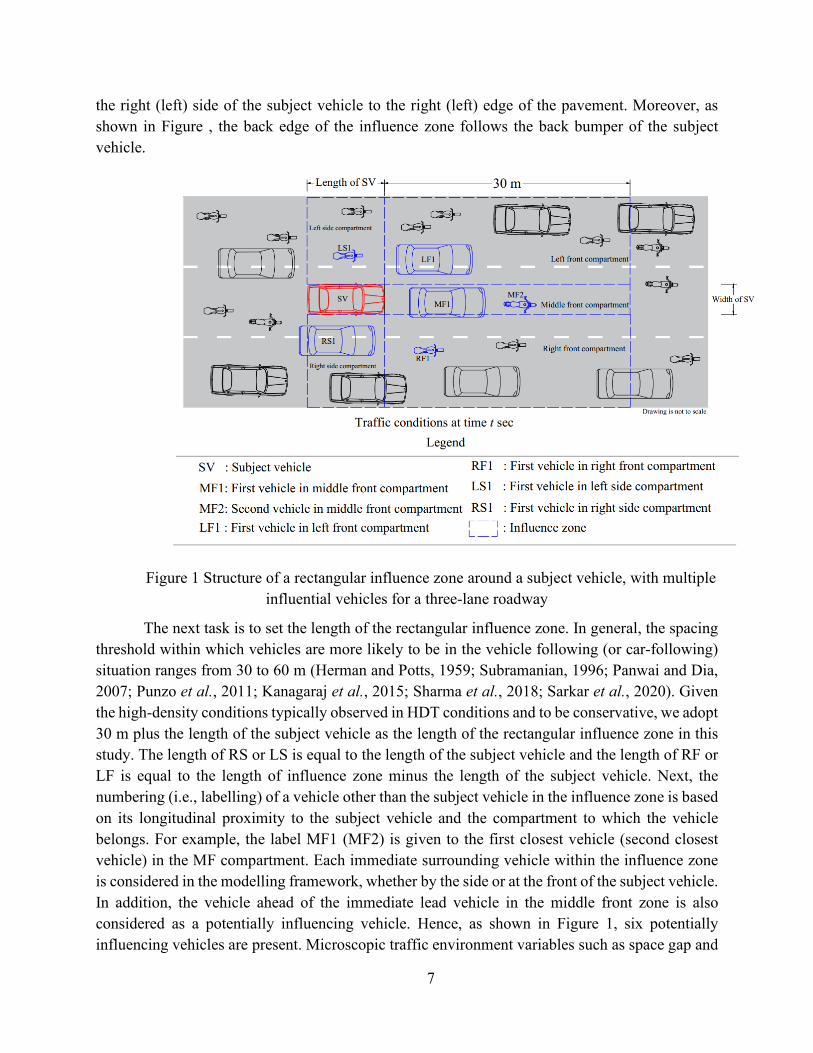
We define the ‘influence zone’ of a vehicle as a hypothetical zone within which the surrounding traffic environment including vehicles, road boundary, stationary traffic control devices, etc. influences the driver behaviour. Different sizes and shapes of influence zones may be explored and empirically investigated to ascertain which size and shape provide the best statistical fit to the observed data as well as the most plausible behavioural insights. However, we restrict ourselves to a rectangular influence zone (as shown in Figure ). The reasons behind choosing a rectangular-shaped influence zone are as follows: a) road boundaries for straight sections can be approximated as two edges of a rectangular shaped influence zone and b) its simple geometric properties provide higher computational tractability. For example, one can easily divide the rectangular influence zone into different compartments to examine the effect of different vehicles on the subject vehicle. For the purpose of demonstration in Figure , the rectangular influence zone is divided into five compartments, namely, middle front (MF), left front (LF), right front (RF), right side (RS), and left side (LS) assuming that the subject vehicle is at the centre of a three-lane roadway. Refer to Figure for a diagrammatic representation of these compartments. As the vehicle’s longitudinal position shifts to the left or right of the roadway width, the influence zone gets truncated accordingly in that direction. In any case, the compartment in the front of the subject vehicle, extending from the subject vehicle’s front bumper to the length of the influence zone is always labeled the MF. When the subject vehicle is at the extreme left edge of the road, there are only three compartments MF, RF, and RS. For the three-lane roadway, the width of the rectangle is approximated to the road pavement width. Particularly, the width of MF is approximated to the width of the subject vehicle, and the width of RF and RS (LF and LS) compartments are set from
7
the right (left) side of the subject vehicle to the right (left) edge of the pavement. Moreover, as shown in Figure , the back edge of the influence zone follows the back bumper of the subject vehicle.
Figure 1 Structure of a rectangular influence zone around a subject vehicle, with multiple influential vehicles for a three-lane roadway
The next task is to set the length of the rectangular influence zone. In general, the spacing threshold within which vehicles are more likely to be in the vehicle following (or car-following) situation ranges from 30 to 60 m (Herman and Potts, 1959; Subramanian, 1996; Panwai and Dia, 2007; Punzo et al., 2011; Kanagaraj et al., 2015; Sharma et al., 2018; Sarkar et al., 2020). Given the high-density conditions typically observed in HDT conditions and to be conservative, we adopt 30 m plus the length of the subject vehicle as the length of the rectangular influence zone in this study. The length of RS or LS is equal to the length of the subject vehicle and the length of RF or LF is equal to the length of influence zone minus the length of the subject vehicle. Next, the numbering (i.e., labelling) of a vehicle other than the subject vehicle in the influence zone is based on its longitudinal proximity to the subject vehicle and the compartment to which the vehicle belongs. For example, the label MF1 (MF2) is given to the first closest vehicle (second closest vehicle) in the MF compartment. Each immediate surrounding vehicle within the influence zone is considered in the modelling framework, whether by the side or at the front of the subject vehicle. In addition, the vehicle ahead of the immediate lead vehicle in the middle front zone is also considered as a potentially influencing vehicle. Hence, as shown in Figure 1, six potentially influencing vehicles are present. Microscopic traffic environment variables such as space gap and

8
relative speed of the subject vehicle with respect to each of these vehicles (side, right front, left front, and middle front) are considered as potential stimuli for the subject vehicle. These are included as explanatory variables in the modelling framework.
3.2. Copula-based Joint Modelling Framework: Formulation and Estimation
Let q be the index representing a driver and let i be the index representing the driver’s discrete manoeuvring choice alternatives ( a = accelerate, d =decelerate, s =maintain same speed), at a time instance t . Note that we suppress the subscript t for time instance for ease in notation. In the proposed model, the manoeuvring choice model component takes a random utility-based discrete choice formulation, and the model component for the extent of the manoeuvre takes the form of a truncated normal regression.
As discussed earlier, dependencies may arise between driver’s discrete and continuous decisions due to the presence of common unobserved factors influencing both decisions. Such dependencies can be captured through statistical correlations between the stochastic components of the equations used to model drivers’ discrete and continuous decisions. In this paper, we use the copula-based approach to incorporate the dependencies. This approach accommodates non-linear and asymmetric dependencies between different types of marginal distributions (which need not follow the same distribution), while also yielding a closed-form expression for the log-likelihood functions to facilitate parameter estimation. By doing so, the approach overcomes the limitations of typical approaches that can accommodate only linear and symmetric dependencies through linear correlation measures (Pearson’s correlation) between marginal distributions of the same type. The copula-based approach has been widely applied in various fields such as econometrics (Cameron et al., 2004; Zimmer and Trivedi, 2006), finance (Embrechts et al., 2002), hydrology (Genest and Favre, 2007) and transportation (Bhat and Eluru, 2009; Spissu et al., 2009). In this paper, we adopted the copula-based joint discrete–continuous modeling framework proposed by Spissu et al. (2009) for simultaneous modeling of the discrete and continuous decisions in the context of driving behaviour. However, the current paper utilizes truncated distributions for the extent of acceleration and deceleration to recognize physical and safety-motivated limits on how much a driver can accelerate or decelerate. In this section, we first describe the discrete choice and continuous model components separately, followed by the copula-based approach to jointly model the decisions.
Before moving further, it is worth noting that although the driving behaviour is characterized as a set of discrete and continuous decisions, the model does not view driving behaviour as a sequential or hierarchical process where drivers decide on the discrete decisions first and then decide on the continuous decisions. Instead, the copula-based approach is employed to jointly model discrete and continuous decisions, where the model views the decisions as simultaneous in that both the discrete and continuous decision are made jointly.

9
3.2.1. Discrete choice component (for the manoeuvring type choice)
The following equation represents the utility structure of the discrete choice component:
* Tqi i qi qiu xβ ε= + (1)
where, *qiu is the utility that the driver of the thq vehicle perceives from choosing a manoeuvring
decision i ; qix is a column vector of attributes (including constant) such as spacing and relative
speed between the subject vehicle and all other vehicles in the influence zone, and roadway geometry features that influence the utility for manoeuvring decision i ; iβ is the corresponding
coefficient vector; and qiε is the random error term representing the distribution of unobserved
factors such as socio-economic characteristics (age, gender, etc.), personality traits (aggressiveness), imperfect driving (perception and estimation errors), etc. influencing *
qiu .
A driver of the vehicle q is assumed to choose a manoeuvring decision i if it is associated with the maximum utility among all manoeuvring decisions; that is, if
{ }
* *
, , ,
*
, , ,
*
, , ,
max
max
max
qi qjj a d s j i
Ti qi qi qjj a d s j i
Tqi qj i qij a d s j i
Tqi i qi
u u
x u
u x
v x
β ε
ε β
β
= ≠
= ≠
= ≠
>
+ >
− > −
> −
(2)
{ }*
, , ,where, maxqi qi qjj a d s j i
v uε= ≠
= − (3)
Equation 2 is equivalent to the multinomial discrete choice model. The distributional assumption of qiε determines the form of the discrete choice probability expression. As discussed
later, this study assumes that the qiε terms are distributed IID type I extreme value across i , which
leads to a multinomial logit (MNL) likelihood expression for the discrete choice component.
3.2.2. Continuous component (for the extent of acceleration/deceleration)
The model component for the extent of acceleration/deceleration takes the form of the typical linear regression model as below:
qi i qiT
qim zα η= + (4)
where, qim is the subject vehicle’s acceleration (deceleration) value at a time instance t
conditional on the decision to accelerate (decelerate). This variable, in turn, is mapped to observed attributes ( )qiz influencing the extent of acceleration (deceleration) through the coefficient vectors
10
iα and a random term qiη that represents the unobserved factors influencing the extent of
acceleration (deceleration). To avoid unrealistically high or low acceleration and deceleration values, we use a truncated normal distribution for qim , which is assumed to arise from a normal
distribution with scale iησ .
3.2.3. Copula-based methodology for joint modelling
A copula is a joint distribution function of standard uniform univariate marginals [0,1]U that associates a stochastic multivariate relationship among the univariate marginals. Given two random variables ( )1 2,B B with marginal cumulative distribution functions ( ) ( )( )1 1 2 2, Fb bF ,
their joint bivariate distribution can be represented as follows:
( ) ( ) ( )( )1 2 1 1 1 2 2 2 , , F b b C u F u Fb bθ= = = (5)
Here, Cθ (copula) is a CDF function which joins ( )1 1F b and ( )2 2F b into a joint distribution.
The individual model components described earlier are brought together, and the likelihood expression of the joint model for a sample of Q vehicles ( ) 1, 2, ,q Q= … is represented as below:
( ) ( ){ }1 1
| qiT Tiqi i qi qi i q
ii
Q I R
L P P m jx v x iv β β= =
= × ∀ ≠ −
> > −∏ ∏ (6)
where, 1 qiR = if the driver of the thq vehicle chooses alternative i , otherwise 0.qiR = I represents
total number of alternatives.
3.2.4. Model estimation
Let qi i qi
i
Tm zh
η
ασ−
= . Hence, the conditional likelihood in Equation (6) can be represented as:
( ) ( )
( ) ( ) ( )1
||
,
T Tqi i qi qi i qi
T Tqi
i
i q
qi q
qi qi qi i qi i
P hm P
P P P
v x v x
v x h v x h
β β
β
η
η ηβ−
=
= −>
> − = > −
− = < − = (7)
A detailed derivation of the above expression is provided in the appendix. As qi i qi
i
Tm zh
η
ασ−
= ,
qii qi
i
mh h mη
η
σσ∂
∂ = ⇒ ∂ = ∂ . Therefore, the joint density in Equation (7) can be expressed as:
( ) ( ),, ,1qi qi
T Tqi i qi vqi i qi
i
P hh Fh
v x xη
ηησ
β β∂=
∂< − = − (8)

11
where ,qi qivF η represents joint cumulative distribution between random variables qiv and qiη . Now,
( )qiP hη = can be expressed as:
( ) ( )1qi i
i
P hh fηη
ησ
= = (9)
Using Equations (8) and (9), we can express Equation (7) as below:
( ) ( ) ( ) ( )1
,1 1| ,
qi qiqi ii i
T T Tqi i qi qi i qi v i qiP
hv xm P f h x hFv x η
ηη
η
βσ
β βσ
−> −
∂ = − ∂ > − − (10)
Let the marginal distributions of qiv and qiη be ( ) .viF and ( ) .iFη , respectively, and the
joint distribution of qiv and qiη be ( ), .,.vi iF η . Subsequently, consider ( ), 1 2 ,vi iF y yη , which can be
expressed as a joint cumulative probability distribution of uniform [0,1] marginal variables 1U
and 2U as below:
( ) ( )( ) ( )( )
( ) ( )( )
, 1 2 1 2
1 11 1 2 2
1 1 2 1
, ,
,
,
vi i qi qi
vi i
vi i
F y y P v y y
P F U y F U y
P U F y U F y
η
η
η
η− −
= < <
= < <
= < <
(11)
Using Sklar’s (1973) theorem, a joint K-dimensional distribution of random variables with the continuous marginal CDF functions ( )k kF y can be generated as below1:
( ) ( )
( )( )
1 2 1 1 1 2
1 1 1 2 2 2
1 1 1 2 2 2
, ,..., Pr , ,...,
Pr ( ), ( ),..., ( )
( ), ( ),..., ( )
k k
k k k
k k k
F y y y Y y Y y Y y
U F y U F y U F y
C u F y u F y u F yθ
= < < <
= < < <
= = = =
(12)
Using above theorem, the joint distribution ( ), ,qi qi
Tv i qiF hxη β− can be expressed by function (.,.)Cθ
such that:
( ) ( )( )', 1 2, , ( )
qi qi qi qi
Tv i qi v i
iiq q
iqF ux h xC u F F hη ηθβ β =− = −= (13)
1For better understanding, ( ) ( ) ( )( ) ( )( )( ) ( )
1
1 2 1 1 2 2
Pr Pr Pr
, ,..., Pr , ,...,k k k k k k k k k k
k k k
F y Y y F U y U F y
C u u u U u U u U uθ
−= < = < = <
= < < <
12
where ( ) .,.Cθ is a copula function and θ is a scalar dependency parameter. This function
characterizes the dependency between qiv and qiη . The joint distribution developed in an above-
discussed manner is used to derive the likelihood expression. As 2 ( )qi
iqu F hη= , we can write:
22 ( )
( )qi
iqi
qi
uu F h h
f hηη
∂= ⇒ ∂ = (14)
Equation (10) can be expressed using Equations (13) and (14) as below (see appendix for details):
( ) ( ) ( ) ( )1 1 2
2
,1 1 | ( )i iq q
qi i i ii
T Tqi i qi qi
ii qih v x v x h
C u uP P f h f
uθ
η ηη η
ησ
βσ
β− ∂
= − ∂ > − >
= −
(15)
Now, substituting Equation (15) into Equation (6), we get
( )1 2
1 1 2
,1 1 qiRi iQ I
q qqi i qi qi i qii i i
q i i i i i
T T C u um z m zL f f i j
uθ
η ηη η η η
α ασ σ σ σ= =
∂ − − = − ∀ ≠ ∂ ∏ ∏ (16)
where,
( )
( ) ( )1
exp
exp exp ln exp1
Ti qi
T Ti qi j qj
j
iqu
x
x x
β
β β
= −
+ ∑
(17)
A detailed derivation of the above expression is provided in the appendix. A truncated normal regression is used to model the continuous part, 2
iqu and can be represented as below:
2
( )
qi
qi i qi i i qi
i iiq
i i qi i i qiT
i i
T T
T
m z L z
u F hU z L z
η η
η
η
η
α ασ σ
α ασ σ
− −Φ −Φ = = − −
Φ −Φ
(18)
where iL and iU are the lower and upper bounds, respectively, on qim . In the empirical context of
this paper, only two discrete choice alternatives – acceleration and deceleration – have a continuous component. Therefore, the log-likelihood function can be written as follows:

13
( ) ( ){ }( ) ( ){ }( ){ }
1
|
|
qa
qd
qs
R
qa a qa qa a qa qa
Q R
qd d qd qd d q
q
T T
T T
Ts
d qdq
R
s qs
P m x v P x v
L P m x v P x v
P x v
β β
β β
β=
> × >
= > × > × >
×
∏ (19)
where, 1qaR = if a driver of thq vehicle takes the acceleration decision, 0 otherwise; 1qdR = if a
driver of thq vehicle takes the deceleration decision, 0 otherwise; and 1qsR = if a driver of thq
vehicle maintains a constant speed, 0 otherwise.
3.2.5. Copula dependence measure
Different copulas offer different levels of ability to capture the dependency between random variables based on the Fréchet–Hoeffding bounds (Bhat and Eluru, 2009). It is useful to construct a scalar metric to measure and compare the dependency implied by different copulas. Traditionally, Pearson’s correlation coefficient is used to measure linear dependence between random variables. However, it does not capture asymmetric dependency among random variables. This limitation has led to the use of the concordance measure approach to describe the dependency. Two random variables are said to be concordant (discordant) if large values of one random variable are related to large (small) values of another random variable, and small values of one variable are related to the small (large) values of another random variable. This results in a dependency measure called Kendall’s τ, which is defined as the probability of concordance minus the probability of discordance. Kendall’s τ satisfies the properties required by Embrechts et al. (2002) for assessing the dependency between random variables, such as taking the zero value for independence (i.e., no dependency). Hence, this study uses Kendall’s τ to characterize and compare the dependency structure. Refer to Embrechts et al. (2002) and Bhat and Eluru (2009) for a detailed discussion on different copulas and their implied dependency measures.
4. DATA AND VARIABLES CONSIDERED IN THE MODEL
4.1. Data
The dataset is a traffic video data of 30 minutes, originally processed by Kanagaraj et al. (2015), from an urban arterial stretch in Chennai with HDT conditions. This is a straight stretch of 245 meters length and 11.2 meters width (and without any entry or exit locations within or nearby). The processed data include individual trajectories of 3005 vehicles (26.6% cars, 56.4% two-wheelers, and 17% other vehicles such as autorickshaws, trucks, and buses), with each vehicle’s trajectory including the spatial position, speed, and acceleration/deceleration values in both the longitudinal and lateral directions at a 0.5 second resolution.
4.2. Description of the Explanatory Variables Considered
To analyze a driver’s decision to accelerate, decelerate, or maintain constant speed and the extent of acceleration or deceleration at a time instance t s, we considered a variety of traffic environment

14
variables at 0.5t − s as sources of stimuli2. These variables can be broadly classified into eight groups, as discussed below, and mentioned in Table 1.
4.2.1. Subject vehicle characteristics
This group includes the subject vehicle’s longitudinal speed. As widely recognized in the literature, a vehicle moving at a higher speed is more (less) likely to decelerate (accelerate) and exhibit a higher (lower) magnitude of deceleration (acceleration) than a vehicle moving at a slower speed.
4.2.2. Stimuli from the first vehicle in the MF compartment (MF1)
These variables include longitudinal space gap and longitudinal speed difference between the subject vehicle and MF1, MF1 vehicle type (which can modify the stimulus), an interaction between vehicle type and the space gap, and an interaction between vehicle type and the relative speed. A vehicle is more likely to accelerate and have higher acceleration value for larger spacing and higher relative speeds (Chandler et al., 1958; Gazis et al., 1959; Edie, 1961; Gazis et al., 1961; May and Keller, 1967; Ahmed, 1999; Toledo, 2003; Choudhury, 2007; Koutsopoulos and Farah, 2012; L. Li et al., 2013). To account for the indirect influence of the second lead vehicle on the subject vehicle, we considered the acceleration of MF1 at t s as an explanatory variable. The subject vehicle is more likely to accelerate (decelerate) if MF1 has been accelerating (decelerating).
4.2.3. Stimuli from the second lead vehicle in the MF compartment (MF2)
This group includes a dummy variable (DM2) for the presence of two or more lead vehicles in the MF compartment, an interaction variable between DM2 and the longitudinal space gap with respect to MF2, and another interaction variable between DM2 and the longitudinal speed difference with respect to MF2. If MF2 is travelling closer to the subject vehicle and at a slower speed than the subject vehicle, the subject vehicle is more likely to decelerate with a higher extent of deceleration. Further, the influence of MF2 on the subject vehicle is likely to be less than that of MF1.
4.2.4. Stimuli from the first lead vehicle in the LF compartment (LF1)
This category includes the following variables a) a dummy variable (DL1) for the presence of one or more vehicles in the LF compartment, b) an interaction between DL1 and the longitudinal space gap with respect to LF1, c) an interaction between DL1 and the longitudinal speed difference with respect to LF1 and d) an interaction between DL1 and the lateral gap between LF1 and MF1. It is likely that the subject driver chooses to decelerate (and decelerate more) if one or more lead vehicles are present in the LF compartment. In addition, if these lead vehicles are nearby the
2 To determine the update time, linear regression models of the observed acceleration values as a function of explanatory variables were built considering different update times – ranging from 0.5 s to 2 s. The model with 0.5 s update time provided the best fit to data and the most intuitive interpretations of the parameter estimates. Therefore, an update time of 0.5 s is used in this study.

15
subject vehicle and are moving at a lower speed, the extent of deceleration is likely to increase. In the same situation, the extent of acceleration is expected to be less if the subject driver accelerates.
4.2.5. Stimuli from the first lead vehicle in the RF compartment (RF1)
These variables include a) a dummy variable (DR1) for the presence of one or more lead vehicles in the RF compartment, b) an interaction between DR1 and the longitudinal space gap with respect to RF1, c) an interaction between DR1 and the longitudinal speed difference with respect to RF1, and d) an interaction between DR1 and the lateral gap between the RF1 and MF1. The subject vehicle’s driver is likely to decelerate and decelerate more if one or more lead vehicles are present in the RF compartment. Additionally, an increase in the magnitude of deceleration is expected if they are located close to the subject vehicle.
4.2.6. Stimuli from the first side vehicle in the LS compartment (LS1)
This group includes a dummy variable (DLS1) to indicate the presence of one or more side vehicles in the LS compartment, an interaction between DLS1 and the lateral space gap between the subject vehicle and LS1, and an interaction between DLS1 and the longitudinal speed difference with respect to LS1. The extent of acceleration is likely to be less if LS1 is laterally closer to the subject vehicle. The speed difference between LS1 and the subject vehicle might also have impact on subject vehicle’s decisions.
4.2.7. Stimuli from the first side vehicle in the RS compartment (RS1)
The stimuli in this group are a dummy variable for the presence of one or more side vehicles in the RS compartment (DRS1), an interaction between DRS1 and the lateral space gap between the subject vehicle and RS1, and an interaction between DRS1 and longitudinal speed difference with respect to RS1. The extent of deceleration is expected to be high if RS1 is located closer to the subject vehicle while, in the case of acceleration, the magnitude of the acceleration is expected to be low. Same as LS1, the longitudinal speed difference between RS1 and the subject vehicle might influence the subject vehicle’s manuevouring decisions.
4.2.8. Road geometry characteristics
Road geometry and other elements such as proximity to the road edge, lane demarcations, curves, and surface deformities also influence driver’s manoeuvring actions (Maurya, 2007; Oviedo-Trespalacios et al., 2017). In this study, the subject vehicle’s proximity to the left edge of the road (i.e., space gap between the left edge of the subject vehicle and the left edge of the road) was included to explore it’s influence on driver behaviour. It is anticipated that vehicles closer to the left edge drive slower than those away from the edge. It is worth noting that the proximity of a vehicle to the left edge of the road can potentially be endogenous to its driver behavior. This is because, in the Indian context, vehicles that intend to travel slow tend to keep to the left of the road. Therefore, one must test the endogeneity of this variable before making inferences on the causal influence of proximity a vehicle to the left edge on its driver behaviour.

16
4.3. Descriptive Statistics
The key descriptive statistics of the processed trajectory dataset are given in Table 1. As can be observed from the table, in most instances, the subject vehicle in HDT condition has at least one vehicle in the LF compartment, possibly because cars typically tend to travel on the right side of the road. Furthermore, the shares of acceleration, deceleration, and maintain same speed states in the Chennai data set are 42.1%, 45.3%, and 12.6%, respectively. This study defines acceleration, deceleration, and constant speed (or maintain same speed) states based on following cut-off values of observed acceleration: (a) observed acceleration greater than +0.1 m/s2 is defined as acceleration state, (b) observed acceleration less than -0.1 m/s2 is defined as deceleration state, and (c) observed acceleration between -0.1 m/s2 and +0.1 m/s2 is defined as constant speed (or maintain same speed) state. In addition, we explored Ozaki’s (1993) definition as well, where vehicles accelerating within ±0.05g, where g = 9.8 m/s2, were considered to be in the constant speed state. Based on this definition, share of acceleration, deceleration, and constant speed states in the Chennai data set are 22.46 %, 23.54 %, and 54.00 %, respectively. It is worth noting here that using Ozaki’s definition results in classification of more than half of the data into the constant speed state, which is not likely to be the case in the current empirical context.
5. MODEL ESTIMATION RESULTS AND DISCUSSION
The model parameters were estimated using the maximum likelihood approach. A variety of empirical models were estimated, including independent models and different copula-based joint models. The independent model ignores dependencies between the discrete choice and continuous choice components. In the joint model, seven different copulas – Gaussian, FGM, Frank, Gumbel, Clayton, Joe, and AMH copulas – were explored to accommodate dependencies between the discrete and continuous choice components. For modelling the extent of acceleration or deceleration, we explored both unbounded normal and truncated normal distributions to determine which distribution results in and better fit and more behaviourally plausible parameter estimates.
To estimate the model parameters, the manoeuvring decisions of the subject vehicle needs to be determined from the observed data. As mentioned earlier, this study classifies various states based on the following cut-off values of acceleration: acceleration greater than +0.1 m/s2 is defined as acceleration state, acceleration less than -0.1 m/s2 is defined as deceleration state, and acceleration between -0.1 m/s2 to +0.1 m/s2 is defined as constant speed state. We also considered the definition by Ozaki (1993), where the maintain same speed state is defined by acceleration values within ±0.05g. However, some of the estimated model parameters were not behaviorally consistent when we considered Ozaki’s (1993) cutoff values. Hence, we do not present and discuss the results based on Ozaki’s definition for constant speed.

17
Table 1 Descriptive statistics of explanatory variables*
Variables HDT conditions Mean Std. dev. Percentage
Dependent variable at t s Acceleration decision -- -- 42.10 Deceleration decision -- -- 45.30 Maintain same speed decision -- -- 12.60
Number of vehicles in different compartments of the influence zone Subject vehicle has 1 or more vehicles in the middle front (MF) compartment -- -- 100.00 Subject vehicle has 2 or more vehicles in the MF compartment -- -- 39.40 Subject vehicle has 1 or more vehicles in the left front (LF) compartment -- -- 89.50 Subject vehicle has 1 or more vehicles in the right front (RF) compartment -- -- 48.92 Subject vehicle has 1 or more vehicles in the left side (LS) compartment -- -- 47.05 Subject vehicle has 1 or more vehicles in the right side (RS) compartment -- -- 22.20 Type of lead vehicle as a motorcycle in MF compartment 27.30
Subject vehicle (SV) characteristics at t-0.5 s
Speed in longitudinal direction (m/s) 12.11 2.48 -- Stimuli from MF1 (first vehicle in MF) at t-0.5 s
Space gap in longitudinal direction (m) 13.94 7.12 -- Relative speed in longitudinal direction (m/s) 0.06 2.70 -- Acceleration at t s (m/s2) -0.02 0.85 --
Stimuli from MF2 (second vehicle in MF) at t-0.5 s Space gap in longitudinal direction (m) 20.99 5.96 -- Relative speed in longitudinal direction (m/s) 0.18 2.86 --
Stimuli from LF1 (first vehicle in LF) at t-0.5 s Space gap in longitudinal direction (m) 8.65 6.94 -- Lateral gap between MF1 and LF1 (m) 2.23 1.32 -- Relative speed in longitudinal direction (m/s) -0.88 3.12 --
Stimuli from RF1 (first vehicle in RF) at t-0.5 s Space gap in longitudinal direction (m) 10.91 8.14 -- Lateral gap between MF1 and RF1 (m) 1.70 1.10 -- Relative speed in longitudinal direction (m/s) 0.67 3.28 --
Stimuli from LS1 (first vehicle in LS) at t-0.5 s Space gap in lateral direction (m) 2.79 1.51 -- Relative speed in longitudinal direction (m/s) -0.86 3.33 --
Stimuli from RS1 (first vehicle in RS) at t-0.5 s Space gap in lateral direction (m) 1.65 0.94 -- Relative speed in longitudinal direction (m/s) 0.63 3.31 --
Road geometry characteristics at t-0.5 s Space gap between left edge of the subject vehicle and left edge of the road (m) 6.31 1.89 --
Total number of cases 17852
*Mean and standard deviation of variables with respect to surrounding vehicles are calculated when vehicles are present in the respective compartment

18
The literature suggests using +4.00 m/s2 as upper bound for acceleration and -4.50 m/s2 as upper bound for deceleration when calibrating the car-following models (HCM, 2000; Saifuzzaman et al., 2015; Sharma et al., 2019). In this study, we used +4.15 m/s2 as upper bound for acceleration and -4.5 m/s2 as upper bound for deceleration. The reason for not considering +4.00 m/s2 as the upper bound for acceleration is that we observed acceleration values up to +4.15 m/s2 in the trajectory data. Therefore, considering only +4.00 m/s2 as the upper bound would require us to discard a good amount of data with acceleration between +4.00 m/s2 and +4.15 m/s2. Therefore, the final truncation thresholds used in this study are [-4.5, -0.1) for deceleration, [-0.1, +0.1] for maintain constant speed, and (+0.1, +4.15] for acceleration.
5.1. Model Selection
Table 2 provides the model fit results for independent and joint models with single leader specifications and multiple leader specifications for unbounded normal and truncated normal distributions of acceleration and deceleration values. This table also presents the statistics for joint models with different copulas. The single leader model specification includes the speed of the subject vehicle, space headway, and relative speed with respect to the immediate lead vehicle, whereas the model with multi-vehicle anticipation considers stimuli from all vehicles that are in the influence zone along with the road geometry characteristics. The different estimated models are not necessarily nested into each other with one as the special case of the other. Therefore, the traditional likelihood ratio test is not applicable to compare the models. Hence, the Bayesian Information Criterion (BIC) metric is employed to compare data fit of the different models. A comparison of BIC values suggests that models with multi-vehicle anticipation perform better (lower BIC values) compared to the single leader model specification. Similarly, models with truncated normal distributions of acceleration and deceleration values perform much better compared to those with unbounded acceleration and deceleration values. Since models with truncation on acceleration and deceleration values provided a better fit than those with unbounded normal distributions, we explored these models for further analysis. Overall, the Frank copula-based joint model with truncated normal distributions for acceleration and deceleration values was found to be the best model with the lowest BIC value for the observed data. Also, the Frank copula model provides the highest adjusted rho-square value.
Table 3 reports the Kendall’s τ values used to examine the level of dependency due to unobserved factors influencing the discrete and continuous decisions. As can be noted from the Kendall’s τ ranges in the table, not all copulas allow the full possible range of dependency. The Gaussian, FGM, Frank, AMH copulas allow both positive and negative dependencies, whereas the other copulas in the table recognize only positive dependency. Further, the FGM copula allows τ values of only up to ± 2/9, whereas the AMH copula allows a maximum τ value of 1/3. Such models that allow only positive dependency or those that allow a limited level of dependency provide a poor fit to observed data as evidenced from the BIC values in Table 2. Further, models with Joe and AMH copulas were encountered with estimation difficulties because of the limited range of the dependency allowed.

19
Table 2 Estimation results with unbounded normal and truncated normal distributions of acceleration/deceleration values*
Joint model with different copula Specifications
Copula dependency parameter (t-statistics)
Loglikelihood at
convergence
BIC value
Adjusted rho-
square Acceleration Deceleration Unbounded normal distributions of acceleration/deceleration values
Independent SL - - -28972.55 58121.32 0.10 ML - - -28244.72 57076.83 0.12
Frank copula SL -4.36 (-16.71) -4.518 (-20.02) -28221.51 56619.24 0.12 ML -4.48 (-17.43) -4.523 (-20.42) -27506.00 55618.98 0.14
Clayton copula SL 8.38 (11.34) 9.266 (11.71) -28043.35 56262.92 0.13 ML 3.05 (62.89) 2.975 (70.42) -27724.51 56056.00 0.14
Joe copula SL 1.00 (10.79) 1.001 (14.84) -28972.55 58121.32 0.10 ML 1.00 (13.39) 1.001 (16.72) -28191.34 57175.66 0.12
AMH copula SL -0.97 (-29.94) -1.000 (-17.64) -28562.49 57301.20 0.11 ML -0.877 (20.8) -0.961 (-32.33) -27906.25 56458.63 0.13
Truncated normal distributions of acceleration/deceleration values
Independent SL -- -- -24839.63 49855.48 0.11 ML -- -- -24131.08 48898.51 0.13
Gaussian copula SL -0.77 (-33.16) -0.82 (-39.10) -25064.92 50306.06 0.10 ML -0.65 (-29.09) -0.69 (-55.89) -24437.07 49422.37 0.12
FGM copula SL -0.99 (-15.37) -1.00 (-20.42) -24832.49 49841.20 0.11 ML -0.77 (-14.50) -0.84 (-29.54) -24118.23 48931.54 0.13
Frank copula SL -4.65 (11.97) -5.20 (16.09) -24726.27 49628.76 0.11 ML -4.23 (12.68) -4.99 (17.73) -24033.43 48673.84 0.14
Gumbel copula SL 1.00 (15.13) 2.19 (15.73) -24867.12 49910.46 0.11 ML 1.00 (17.58) 1.00 (21.93) -24120.73 48965.91 0.13
Clayton copula SL 2.40 (21.32) 2.49 (23.70) -24900.68 49977.59 0.11 ML 2.27 (23.53) 2.42 (24.63) -24329.78 49178.42 0.13
SL-Single leader specification, ML- Multiple leader specification, *The joint copula models with convergence problem are not reported in the table.
The Kendall’s τ values from the models that allow both positive and negative dependency (Gaussian, FGM, and Frank copula models) reveal that all the dependency parameters are significantly different from zero, indicating a significant presence of unobserved factors that affect drivers' discrete manoeuvring decisions and the extent of acceleration/deceleration. The most striking result is the negative dependency (or the negative Kendall’s τ value) suggesting that the unobserved factors that increase (decrease) the propensity to choose a discrete decision make the driver decrease (increase) the extent of that discrete decision. We found similar results when we used Ozaki’s (1993) cutoff value of ±0.05g for acceleration magnitude to decide instances of constant speed following. This consistent result across various settings implies that the unobserved factors that make a driver accelerate or decelerate more frequently (less frequently) also make that driver to accelerate or decelerate less (more). The negative dependency can be explained based on unobserved factors such as driver aggressiveness, as follows. As aggressive drivers aim for small gaps with respect to their lead vehicles (Tasca, 2000; Lajunen and Parker, 2001; Abou-Zeid et al., 2011), they tend to accelerate and decelerate more frequently than other vehicles (Ahn and Rakha, 2009). Aggressive drivers do not let the space gap grow much by frequently accelerating to close

20
in on their lead vehicles and then decelerating to maintain the gap. Since such behaviour makes them accelerate and decelerate more frequently and maintain close gaps, the amount of acceleration or deceleration they can attain at any instance tends to be smaller than that of other drivers who tend to wait for longer gaps. Next, one can observe from Table 3 that the magnitude of Kendall’s τ value is slightly higher for the dependency between the deceleration decision and the extent of deceleration (than that for acceleration related decisions), suggesting that there is a higher level of dependency associated with the deceleration related decisions than that with acceleration related decisions.
Table 3 Kendall’s dependency measure for different copulas
Copula
Copula parameter
(θ )’s range
Kendall’s τ Kendall’s τ range
Kendall’s τ for
acceleration
Kendall’s τ for
deceleration
Gaussian [-1,1] ( )2τ arcsin θπ
= [-1,1] -0.450 -0.485
FGM [-1,1] 2τ9θ= 2 2 ,
9 9−
-0.171 -0.187
Frank [ , ]−∞ ∞ ( )4τ 1 1 FD θ
θ= − − ,
( )0
1 1nk wFraw
D dwe
wθ
θθ =
=−∫
[-1,1] -0.405 -0.456
Gumbel [1, )∞ 1τ 1 θ
= − [0,1) 0.001 0.001
Clayton (0, )∞ τ2
θθ
=+
(0,1) 0.532 0.548
Joe [1, )∞ ( )4τ 1 JD θ
θ= + ,
( )( ) ( )1
10
ln 1 1Joe
w
w wD
wdw
θ θ
θθ −=
− − = ∫ [0,1 ) CP CP
AMH [ 1,1]− ( ) ( )( )2
2
2 1 log 1τ 1
3
θ θ θ
θ
− − += −
5 8ln 2 1, 3 3
−
CP CP
CP-Convergence problems encountered in estimating the model
5.2. Final Model Estimation Results and Discussion
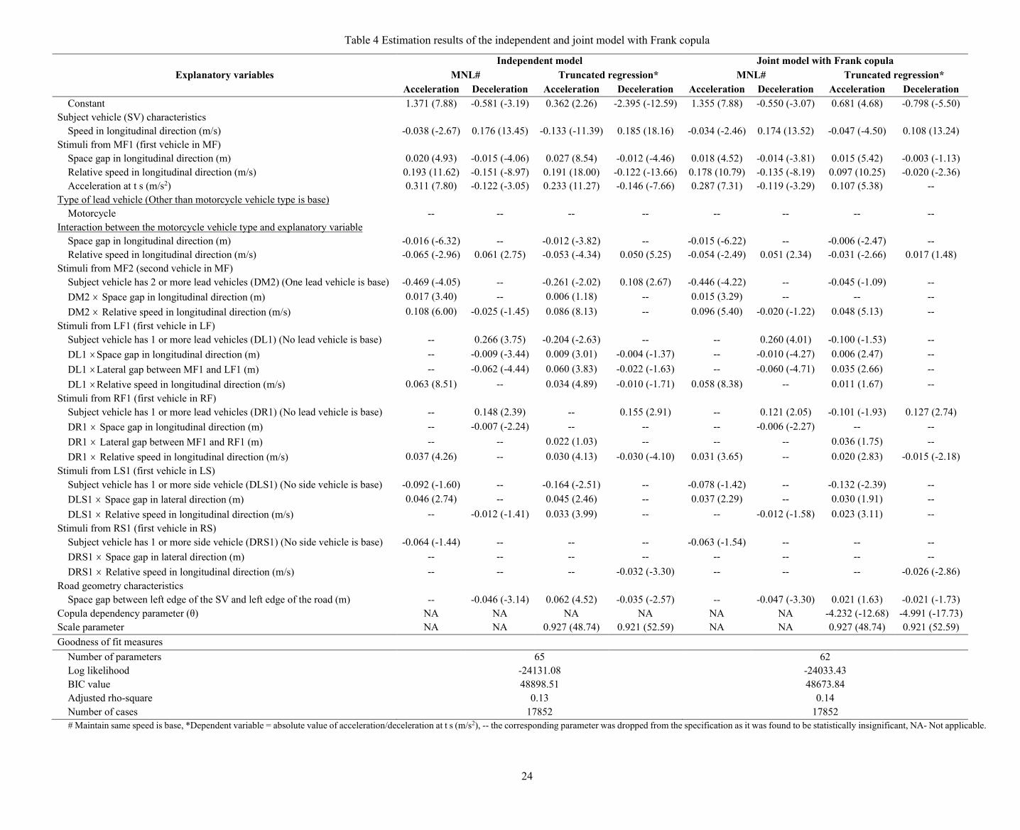
Since the Frank copula model provides the best fit to observed data as well as more behaviorally plausible interpretations, we discuss the estimation results of that model in detail and compare it with the independent model. The estimation results of the independent model and joint model with Frank copula are provided in Table 4.

21
A comparison between the Frank copula and independent models suggests that the parameter estimates from the copula-based joint model have lower t-statistic values when compared to those in the independent model. This is especially so for the continuous components of the model (i.e., for the parameter estimates corresponding to the extent of acceleration and the extent of deceleration). Also, although not reported here, a comparison of various copula-based joint models reveals that the t-statistic values of parameter estimates in the continuous component were found to be smaller for models with stronger copula dependency values. This implies that ignoring negative dependency between the discrete and continuous components may lead to overestimation of the influence of some factors (along with their t-statistic values) on the extent of acceleration or deceleration. This may also lead to a false conclusion that the parameter estimates are more precise. Hence, there will be a tendency not to reject the null hypothesis (parameter does not have an impact on driver’s decisions) when it should be rejected. Another point to note is that not all factors that influence the discrete decision (accelerate, decelerate, or maintain constant speed) influence the continuous decisions (how much to accelerate or decelerate) or vice versa. In essence, this discussion highlights the need to model the discrete and continuous components of driver behavior decisions separately but also reinforces the case for considering the dependency between discrete and continuous decisions. Moreover, the joint model is parsimonious (three less parameters than those in the independent model) and at the same time offers greater explanatory power than the independent model, as indicated by goodness of fit metrics at the end of Table 4.
Now, we discuss the influence of different variables on a subject vehicle driver’s decisions. In line with expectation, the parameter estimates of the subject vehicle speed variable suggest that vehicles travelling at slower longitudinal speeds are more likely to accelerate (and accelerate more) than vehicles travelling at higher speeds. Similar findings are reported in Siuhi (2009) and Subramanian (1996). Next, the parameter estimates for space headway with respect to MF1 are statistically significant at 1% level of significance for the decisions to accelerate, decelerate, and the extent of acceleration. These results indicate that the subject vehicle is more likely to accelerate and have a higher acceleration value for larger space gaps with respect to the MF1. On the other hand, smaller space gaps make the driver more likely to decelerate and decelerate more. The consideration of dependency between discrete and continuous decisions makes space headway less influential on the extent of deceleration (this parameter had a stronger influence with a higher t-statistic value in the independent model). Next, the parameter estimates of the relative speed are statically significant at 1% significance level in all discrete and continuous decisions with consistent signs as expected. A positive parameter in acceleration decisions (negative parameter in deceleration decisions) suggests that the subject vehicle is more likely to accelerate (decelerate) and accelerate (decelerate) more when MF1 is moving faster than the subject vehicle. The findings are also consistent with those in Koutsopoulos and Farah (2012) in the context of the discrete decision of whether to accelerate or decelerate. For example, the probability of acceleration state increases with an increase in the relative speed between the lead vehicle and the following vehicle.
22
We have also considered the indirect effect of MF2 (in addition to the direct effect of MF2 discussed later) on the subject vehicle by considering the acceleration of the MF1. It can be seen from Table 4 that this variable is statistically significant at 1% significance level in the decision to accelerate, decision to decelerate and the extent of acceleration. The sign of the parameter estimate for this variable is positive in both acceleration decisions and the extent of acceleration, whereas negative in the decision to decelerate. This indicates that the subject vehicle is more likely to accelerate and accelerate more when MF1 is accelerating, and the subject vehicle is more likely to decelerate when MF1 is decelerating.
Furthermore, the effect of the type of immediate lead vehicle was also examined. The parameter for interaction between vehicle type of MF1 and space gap with respect to MF1 has a negative coefficient in the decision to accelerate and the extent of acceleration indicating that the subject vehicle is less likely to accelerate and would accelerate less if MF1 is motorcycle instead of other vehicle types. Similar conclusions can be made for the interaction variable between vehicle type and the relative speed with respect to MF1. Choudhury and Islam (2016) and Ravishankar and Mathew (2011) also report similar influences of the type of lead vehicles on drivers’ extent of acceleration.
The estimation results reveal that six out of twelve parameter estimates on the variables related to MF2 are statistically significant. Importantly, no parameter estimate is statistically significant in the extent of deceleration, implying that the presence of a second lead vehicle does not impact the extent of deceleration. Similar observations can be made in the context of variables related to LF1, RF1, LS1 and RS1. Specifically, the extent of deceleration is not influenced as much by the variables corresponding to all these vehicles than by the variables corresponding to MF1. That is, drivers’ decisions on the extent of acceleration are governed by multiple vehicles ahead, whereas their decisions on the extent of deceleration are likely to be affected much more by the immediate lead vehicle than that of other vehicles in the influence zone. Several studies (Bexelius, 1968; Lenz et al., 1999; Hoogendoorn and Ossen, 2006) also confirm that drivers respond to the multiple vehicles directly ahead, but we are not aware of studies that report such nuanced findings for the influence of different lead vehicles on driving behaviours.3
We now turn to the effect of the vehicles in the left front (LF1), right front (RF1), left side (LS1), and right side (RS1) on the subject vehicle’s driving behaviour. For each of these vehicles, the parameter estimates reported in Table 4 are in line with our expectations. For example, the parameter estimates for the relative speed with respect to LF1 and those with respect to RF1 take a positive sign in the decisions to accelerate and the extent of acceleration. This implies that the likelihood of acceleration increases with an increase in relative speed between the influencing
3 The independent model estimated in this study spuriously shows the influence of variables related MF2 on the extent of subject vehicle’s deceleration. The joint model, on the other hand, shows no influence of variables related to MF2 on the extent of deceleration. These results highlight the need for considering dependency between discrete and continuous decisions of whether to accelerate/decelerate and how much to do so.

23
vehicles (LF1 and RF1) and the subject vehicle. Furthermore, the parameter estimates related to the lateral gap with respect to LS1 indicate that larger (smaller) space gaps are associated with a higher (lower) likelihood of acceleration as well as higher (lower) extent of acceleration. Additionally, the parameter estimates of relative speed with respect to LS1 suggest that drivers are less likely to decelerate and the extent of acceleration increases with an increase in the relative speed between LS1 and the subject vehicle. Also, the parameter estimate for relative speed with respect to RS1 indicates that an increase in the relative speed with respect to RS1 decreases the extent of deceleration. Such findings indicate that drivers’ anticipation of traffic situation and their response depends on vehicles on the side in addition to vehicles ahead. Hence, one can conclude that vehicles, which are in the left front, right front, left side and right side, are also likely to affect a driver’s decisions.
The gap between the subject vehicle and the left edge of the road was also found to have a significant influence on driving decisions. A smaller gap between the vehicle and the road edge makes car drivers tend to decelerate more. This is intuitively aligned with our expectations since in HDT scenarios, for example, in the Indian driving context, low speed traffic opts the left side of the road whereas high speed traffic is on the right side. As discussed earlier, this variable can potentially be endogenous to drivers’ decisions to acceleration and deceleration. To correct for such endogeneity, we used the control function method. Specifically, we first regressed the vehicles’ distance to the road's left and then used the residual from this regression as another variable in the copula-based joint model. The coefficient of the residual turned out to be statistically insignificant in both discrete and continuous decision equations of the joint model. Therefore, we dropped the endogeneity correction from the final specification of the proposed model.
It is worth noting here that one cannot include another variable titled gap from the right edge of the road, as such a model cannot be identified since the gap to the left edge and that to the right edge (along with vehicle width) would add up to a constant (road width). Importantly, the modeling framework is general enough to allow for the inclusion of roadway geometry elements such as spacing from the curb, presence and spacing of any fixed objects on the road, and irregularities in the geometry as more empirical data becomes available from such varied conditions.
To further demonstrate the importance of considering multi-vehicle anticipation, additional empirical models were estimated by cumulatively including stimuli from one vehicle at a time until all stimuli from all surrounding vehicles in the influence zone were included in the model. Log-likelihood ratio tests were performed to compare these different models (see Table 5). As can be observed from the test results in Table 5, considering the influence of multiple vehicles improves the model fit. In fact, the model fit improved due to the consideration of each (and every) additional influencing vehicle. This observation underscores the importance of considering multiple-vehicle anticipation in driver behavior modelling. This finding also validates the existence of the influence zone for each vehicle.
24
Table 4 Estimation results of the independent and joint model with Frank copula
Explanatory variables Independent model Joint model with Frank copula
MNL# Truncated regression* MNL# Truncated regression* Acceleration Deceleration Acceleration Deceleration Acceleration Deceleration Acceleration Deceleration
Constant 1.371 (7.88) -0.581 (-3.19) 0.362 (2.26) -2.395 (-12.59) 1.355 (7.88) -0.550 (-3.07) 0.681 (4.68) -0.798 (-5.50) Subject vehicle (SV) characteristics
Speed in longitudinal direction (m/s) -0.038 (-2.67) 0.176 (13.45) -0.133 (-11.39) 0.185 (18.16) -0.034 (-2.46) 0.174 (13.52) -0.047 (-4.50) 0.108 (13.24) Stimuli from MF1 (first vehicle in MF)
Space gap in longitudinal direction (m) 0.020 (4.93) -0.015 (-4.06) 0.027 (8.54) -0.012 (-4.46) 0.018 (4.52) -0.014 (-3.81) 0.015 (5.42) -0.003 (-1.13) Relative speed in longitudinal direction (m/s) 0.193 (11.62) -0.151 (-8.97) 0.191 (18.00) -0.122 (-13.66) 0.178 (10.79) -0.135 (-8.19) 0.097 (10.25) -0.020 (-2.36) Acceleration at t s (m/s2) 0.311 (7.80) -0.122 (-3.05) 0.233 (11.27) -0.146 (-7.66) 0.287 (7.31) -0.119 (-3.29) 0.107 (5.38) --
Type of lead vehicle (Other than motorcycle vehicle type is base) Motorcycle -- -- -- -- -- -- -- --
Interaction between the motorcycle vehicle type and explanatory variable Space gap in longitudinal direction (m) -0.016 (-6.32) -- -0.012 (-3.82) -- -0.015 (-6.22) -- -0.006 (-2.47) -- Relative speed in longitudinal direction (m/s) -0.065 (-2.96) 0.061 (2.75) -0.053 (-4.34) 0.050 (5.25) -0.054 (-2.49) 0.051 (2.34) -0.031 (-2.66) 0.017 (1.48)
Stimuli from MF2 (second vehicle in MF) Subject vehicle has 2 or more lead vehicles (DM2) (One lead vehicle is base) -0.469 (-4.05) -- -0.261 (-2.02) 0.108 (2.67) -0.446 (-4.22) -- -0.045 (-1.09) -- DM2 × Space gap in longitudinal direction (m) 0.017 (3.40) -- 0.006 (1.18) -- 0.015 (3.29) -- -- -- DM2 × Relative speed in longitudinal direction (m/s) 0.108 (6.00) -0.025 (-1.45) 0.086 (8.13) -- 0.096 (5.40) -0.020 (-1.22) 0.048 (5.13) --
Stimuli from LF1 (first vehicle in LF) Subject vehicle has 1 or more lead vehicles (DL1) (No lead vehicle is base) -- 0.266 (3.75) -0.204 (-2.63) -- -- 0.260 (4.01) -0.100 (-1.53) -- DL1 ×Space gap in longitudinal direction (m) -- -0.009 (-3.44) 0.009 (3.01) -0.004 (-1.37) -- -0.010 (-4.27) 0.006 (2.47) -- DL1 ×Lateral gap between MF1 and LF1 (m) -- -0.062 (-4.44) 0.060 (3.83) -0.022 (-1.63) -- -0.060 (-4.71) 0.035 (2.66) -- DL1 ×Relative speed in longitudinal direction (m/s) 0.063 (8.51) -- 0.034 (4.89) -0.010 (-1.71) 0.058 (8.38) -- 0.011 (1.67) --
Stimuli from RF1 (first vehicle in RF) Subject vehicle has 1 or more lead vehicles (DR1) (No lead vehicle is base) -- 0.148 (2.39) -- 0.155 (2.91) -- 0.121 (2.05) -0.101 (-1.93) 0.127 (2.74) DR1 × Space gap in longitudinal direction (m) -- -0.007 (-2.24) -- -- -- -0.006 (-2.27) -- -- DR1 × Lateral gap between MF1 and RF1 (m) -- -- 0.022 (1.03) -- -- -- 0.036 (1.75) -- DR1 × Relative speed in longitudinal direction (m/s) 0.037 (4.26) -- 0.030 (4.13) -0.030 (-4.10) 0.031 (3.65) -- 0.020 (2.83) -0.015 (-2.18)
Stimuli from LS1 (first vehicle in LS) Subject vehicle has 1 or more side vehicle (DLS1) (No side vehicle is base) -0.092 (-1.60) -- -0.164 (-2.51) -- -0.078 (-1.42) -- -0.132 (-2.39) -- DLS1 × Space gap in lateral direction (m) 0.046 (2.74) -- 0.045 (2.46) -- 0.037 (2.29) -- 0.030 (1.91) -- DLS1 × Relative speed in longitudinal direction (m/s) -- -0.012 (-1.41) 0.033 (3.99) -- -- -0.012 (-1.58) 0.023 (3.11) --
Stimuli from RS1 (first vehicle in RS) Subject vehicle has 1 or more side vehicle (DRS1) (No side vehicle is base) -0.064 (-1.44) -- -- -- -0.063 (-1.54) -- -- -- DRS1 × Space gap in lateral direction (m) -- -- -- -- -- -- -- -- DRS1 × Relative speed in longitudinal direction (m/s) -- -- -- -0.032 (-3.30) -- -- -- -0.026 (-2.86)
Road geometry characteristics Space gap between left edge of the SV and left edge of the road (m) -- -0.046 (-3.14) 0.062 (4.52) -0.035 (-2.57) -- -0.047 (-3.30) 0.021 (1.63) -0.021 (-1.73)
Copula dependency parameter (θ) NA NA NA NA NA NA -4.232 (-12.68) -4.991 (-17.73) Scale parameter NA NA 0.927 (48.74) 0.921 (52.59) NA NA 0.927 (48.74) 0.921 (52.59) Goodness of fit measures
Number of parameters 65 62 Log likelihood -24131.08 -24033.43 BIC value 48898.51 48673.84 Adjusted rho-square 0.13 0.14 Number of cases 17852 17852 # Maintain same speed is base, *Dependent variable = absolute value of acceleration/deceleration at t s (m/s2), -- the corresponding parameter was dropped from the specification as it was found to be statistically insignificant, NA- Not applicable.

25
Table 5 Estimation results for different number of lead vehicles in the model.
Goodness of fit measures of models considering influence of …
Influence of 1 lead vehicle in middle front compartment
Influence of 1 lead vehicle in middle front compartment by considering type of lead vehicle and interaction with other stimuli from same vehicle
Influence of 2 vehicles in middle front compartment*
Influence of 2 vehicles in middle front and 1 in left front compartment*
Influence of 2 vehicles in middle front, 1 in left front, 1 in right front compartment*
Influence of 2 vehicles in middle front, 1 in left front, 1 in right front, 1 on left side compartment*
Influence of 2 vehicles in middle front, 1 in left front, 1 in right front, 1 on left side, 1 on right side compartment*
Influence of 2 vehicles in middle front, 1 in left front, 1 in right front, 1 on left side, 1 on right side compartment and road geometry characteristics*
Model number Model 1 Model 2 Model 3 Model 4 Model 5 Model 6 Model 7 Model 8 Log likelihood -24726.27 -24354.95 -24238.55 -24150.36 -24068.42 -24054.68 -24046.29 -24033.43
Number of significant parameters
20 29 35 43 51 57 59 62
Number of restrictions -- 9 6 8 8 6 2 3
LLR -- 742.64 232.79 176.38 163.88 27.49 16.78 25.71 χ2 at 95 %
confidence level -- 16.92 12.59 15.51 15.51 12.59 5.99 7.81
Remark -- Model 1 is rejected compared to model 2
Model 2 is rejected
compared to model 3
Model 3 is rejected compared to model
4
Model 4 is rejected compared to model
5
Model 5 is rejected compared to model 6
Model 6 is rejected compared to model 7
Model 7 is rejected compared to model 8
Number of cases 17852
*Type of lead vehicle and interaction with other stimuli from same vehicle is also considered in the model specification

26
The empirical model presented here extends the current understanding of driving behaviour in HDT conditions. The results underscore the importance of considering multi-vehicle anticipation to model driving behaviour, where multiple vehicles within the influence zone of the subject vehicle influences its driver’s decisions. Doing so can help improve the realism of driver behaviour models for HDT traffic streams. Further, the literature identifies other advantages of considering multi-vehicle anticipation such as an increase in the stability of traffic flow, compensation for the adverse effect induced by reaction delays, and better representation of fundamental traffic flow diagrams (Lenz et al., 1999; Treiber et al., 2006; Wang et al., 2006; Ossen, 2008; Peng and Sun, 2010). Moreover, as driver behaviour models are vital for traffic flow analysis, traffic safety analysis, and traffic emissions estimation, employing the proposed model can assist in getting more realistic results from such analyses. Given the potential gains from considering multi-vehicle anticipation, the available driver assistance systems technology for HDT conditions can potentially benefit from including multi-vehicle anticipation-based prediction algorithms. In addition to HDT conditions, the proposed model can be applied in homogenous traffic conditions as well, since (a) multi-vehicle anticipation has been found in homogenous conditions too (Bexelius, 1968; Lenz et al., 1999; Hoogendoorn and Ossen, 2006; Treiber et al., 2006; Peng and Sun, 2010), (b) longitudinal movements dominate in these conditions, and (c) the modelling framework is generic and transferrable. Furthermore, using the proposed model to simulate human-driven vehicles in a mixed traffic of human-driven and autonomous vehicles will likely improve the realism of the simulated mixed traffic environment. Such a simulation environment can potentially offer a more robust investigation of autonomous vehicles’ trajectory planning algorithms.
6. VALIDATION
A validation exercise was performed on a hold-out dataset of 5,000 vehicle manoevures to assess the efficacy of the proposed model in predicting driver’s discrete and continuous decisions at an aggregate level. To do so, the following procedure was followed for simulating the driver’s discrete and continuous decisions for each of the 5,000 data points ( 1, 2, ..., 5,000)q = .
1. Simulate the discrete decisions: To simulate discrete decisions of acceleration, deceleration, or maintain same speed, we used the following two-step approach:
(1a). Calculate the probability of each possible discrete choice decision ( , ,i a d s= ) using the following multinomial logit expression.
( )( )
exp; , ,
exp
Ti qi
qi Tj qj
j
xP i a d s
x
β
β= =∑
(20)
(1b). Use the above calculated discrete choice probabilities to simulate the discrete decision of acceleration ( i a= ), deceleration ( i d= ), or maintain constant speed ( i s= ). This can
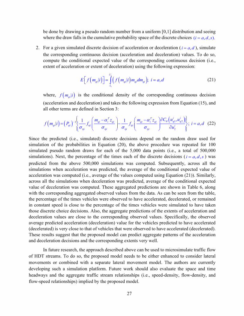
27
be done by drawing a pseudo random number from a uniform [0,1] distribution and seeing where the draw falls in the cumulative probability space of the discrete choices ( , , ).i a d s=
2. For a given simulated discrete decision of acceleration or deceleration ( ,i a d= ), simulate the corresponding continuous decision (acceleration and deceleration) values. To do so, compute the conditional expected value of the corresponding continuous decision (i.e., extent of acceleration or extent of deceleration) using the following expression:
( ) ( )( )| | ; ,i
i
U
qi qi qi qiL
E f m i f m i m dm i a d = = ∫ (21)
where, ( )|qif m i is the conditional density of the corresponding continuous decision
(acceleration and deceleration) and takes the following expression from Equation (15), and all other terms are defined in Section 3:
( ) ( ) ( )1 21
2
,1 1| ; ,i iT Tq qqi i qi qi i qi
qi qi i i ii i i i
C u um z m zf m i P f f i a d
uθ
η ηη η η η
α ασ σ σ σ
− ∂ − − = − = ∂
(22)
Since the predicted (i.e., simulated) discrete decisions depend on the random draw used for simulation of the probabilities in Equation (20), the above procedure was repeated for 100 simulated pseudo random draws for each of the 5,000 data points (i.e., a total of 500,000 simulations). Next, the percentage of the times each of the discrete decisions ( , ,i a d s= ) was predicted from the above 500,000 simulations was computed. Subsequently, across all the simulations when acceleration was predicted, the average of the conditional expected value of acceleration was computed (i.e., average of the values computed using Equation (21)). Similarly, across all the simulations when deceleration was predicted, average of the conditional expected value of deceleration was computed. These aggregated predictions are shown in Table 6, along with the corresponding aggregated observed values from the data. As can be seen from the table, the percentage of the times vehicles were observed to have accelerated, decelerated, or remained in constant speed is close to the percentage of the times vehicles were simulated to have taken those discrete choice decisions. Also, the aggregate predictions of the extents of acceleration and deceleration values are close to the corresponding observed values. Specifically, the observed average predicted acceleration (deceleration) value for the vehicles predicted to have accelerated (decelerated) is very close to that of vehicles that were observed to have accelerated (decelerated). These results suggest that the proposed model can predict aggregate patterns of the acceleration and deceleration decisions and the corresponding extents very well.
In future research, the approach described above can be used to microsimulate traffic flow of HDT streams. To do so, the proposed model needs to be either enhanced to consider lateral movements or combined with a separate lateral movement model. The authors are currently developing such a simulation platform. Future work should also evaluate the space and time headways and the aggregate traffic stream relationships (i.e., speed-density, flow-density, and flow-speed relationships) implied by the proposed model.

28
Table 6 Observed and predicted aggregate acceleration and deceleration decisions in a hold-out sample (N = 5,000 data records)
Discrete and continuous decisions Observed Predicted Percentage of instances vehicles accelerated (discrete choice) 41.9% 41.3%
Average acceleration (average of conditional expected acceleration calculated using Equation (21)) if the discrete decision is acceleration 0.75 m/s2 0.74 m/s2
Percentage of instances vehicles decelerated (discrete choice) 44.9% 46.5%
Average deceleration (average of conditional expected deceleration calculated using Equation (21)) if the discrete decision is deceleration 0.71 m/s2 0.72 m/s2
Percentage of instances vehicles maintained same speed 13.2% 12.3%
7. CONCLUSIONS AND FUTURE RECOMMENDATIONS
This study proposes a multi-vehicle anticipation and copula-based discrete-continuous choice modelling framework for describing driver behaviour in HDT conditions. To incorporate the impact of multi-vehicle anticipation, we introduce the concept of influence zone around a subject vehicle and consider stimuli from all vehicles and other objects within the influence zone. Further, driving decisions are characterized as combination of discrete and continuous components. The discrete component involves the decision to accelerate, decelerate, or maintain a constant speed and the continuous component involves the decision of how much to accelerate or decelerate. The proposed copula-based joint modelling framework allows a flexible error dependency structure between driver’s discrete and continuous decisions. Additionally, truncated distributions are employed for the continuous model components to avoid the prediction of unrealistically high acceleration or deceleration values.
The model estimation has been carried out using a vehicle trajectory dataset from Chennai, India. To capture the dependency structure between the driver’s manoeuvring decision and its extent, various copula functions including Gaussian, FGM, Frank, Gumbel, Clayton, Joe, and AMH have been employed in this study. Overall, the Frank copula model with truncated distributions that consider bounds for acceleration and deceleration values performed better than all other models estimated in the study.
The empirical results of this study enhance the current understanding of driving behaviours in HDT conditions in several ways. First, the results demonstrate the importance of considering multi-vehicle anticipation for describing driving behaviour in HDT conditions. Specifically, the results lend credence to the idea of an influence zone around the vehicle and corroborate our hypothesis that driving behaviour is influenced by multiple vehicles within the influence zone of the subject vehicle. Further, drivers in HDT conditions not only consider vehicles that are ahead of their vehicle but also consider those vehicles that are on either side. At the same time, while the
29
drivers’ decision to accelerate and the extent of acceleration is governed by multiple vehicles ahead, their decision on the extent of deceleration is likely to be affected more by the immediate lead vehicle than other vehicles in the influence zone. Such nuanced findings have not been reported by other studies that considered multi-vehicle anticipation in driving behaviour.
Second, most of the earlier studies in the literature model driver behaviour as a single continuum, where the discrete decisions (of whether to accelerate, decelerate, or remain in constant speed) and continuous decisions (how much to accelerate or decelerate) are not treated separately. However, this study demonstrates that driving behaviour is more complex. The results support the notion that discrete and continuous decisions are separate and the factors influencing the discrete decisions might be different or may influence the continuous decisions differently. Specifically, not all traffic environment variables found to influence the discrete decisions were found influential on continuous decisions (or how much to accelerate or decelerate) and vice versa. Moreover, the influence of several variables was found to be stronger on the decision to accelerate or decelerate than on the decision of how much to accelerate or decelerate. This suggests that the discrete and continuous decisions likely require different cognitive efforts by drivers and are influenced in different ways by the traffic environment variables. Such findings add to our understanding of driver decision making process and driving task performance.
Third, the results indicate the presence of significant unobserved factors contributing to the negative dependency between the driver’s discrete and continuous decisions. This suggests that the unobserved factors that increase (decrease) the propensity to accelerate/decelerate are more likely to decrease (increase) the extent of acceleration/deceleration. When compared to the estimation results of an independent model that ignores such dependencies, the copula-based joint models offer a statistically superior goodness-of-fit and more plausible behavioural interpretations. This highlights the importance of jointly modeling the discrete and continuous decisions. In addition, employing truncated normal distributions to model acceleration and deceleration values not only led to a significant improvement in the model fit but also prevents the possibility of unrealistically high acceleration or deceleration values.
Note that the current study focuses only on the longitudinal movement of cars. Simultaneous modelling of longitudinal and lateral movements is a natural and important extension of this work. Doing so will help in building a model that can comprehensively represent driving behaviour in HDT conditions. Equally useful would be the development of a simulator to apply the proposed model in conjunction with a lateral movement model for simulation of traffic flow in HDT conditions. Further, future research should relax the assumption of a rectangular influence zone of fixed size. The shape and size of the influence zone might be different for different drivers. Since the influence zone cannot be observed in the data, one possible way to consider inter-driver heterogeneity in influence zones is to consider latent classes for different shapes/sizes of influence zones (and probabilistically associate the subject vehicle and driver characteristics, traffic stream variables, etc. to different influence zones). The driving decisions can then be modelled conditional on the influential zone using the approach followed in latent

30
class choice models. Another direction for future research is to evaluate the efficacy of the proposed modelling framework for homogenous traffic conditions, because multiple-vehicle anticipation has been observed in homogenous traffic conditions as well. Also, it would be interesting to identify the aggressive and non-aggressive driver profiles in the dataset and incorporate these differences in the driving behaviour in the modelling framework.
Acknowledgments
The authors are grateful to Caleb Ronald Munigety for his valuable inputs during the early stages of this study and Partha Chakroborty for his insights on the interpretation of empirical results. The authors are thankful to Kanagaraj et al. (2015) for sharing the trajectory data used in this study. Three anonymous reviewers provided helpful comments on an earlier version of the paper.
Appendix A. Derivations
Assuming qi i qi
i
Tm zh
η
ασ−
= , the conditional probability in Equation (6) can be expressed as:
( ) ( )( ) ( )( ) ( ) ( )( ) ( ) ( )( )
1
1
1
1
|
1
|
,
|
|
T Tqi i qi qi i qi
T Tqi i qi qi i qi
T Tqi i qi q
q
qi q
i i qi
T Tqi i qi i
i
i qi
Tqi i q
i
qi
q qi
q
i
i qi
P v x h v x
v x v x h
v x v x h
P
h
v x v x h h
v
m P
P P
P P P
P P
P x P
η
η
η η
η η
η
β β
β β
β β
β β
β
−
−
−
−
=
=
=
> − = > −
> − > − =
> − > − = =
> − < − = = −
=
>= − ( ) ( ) ( )( ) ( ) ( )1
|
,
Tqi i qi
T Tqi i
qi q
qi qi i qi
i qi
qi qi
h
P
v x h h
v x hP v x
P P
P h
β
β
η η
βη η−
−
= < − = =
>
−− = < − = =
(23)
The derivation for the expression given in Equation (15) is as follows:
( )
( ) ( ) ( )
( ) ( ) ( )( )
( ) ( )
1
1
1 22
1
,1 1
1 1 ( ) , ( )
,
1
1
|
qi qi
qi qi
qi
ii i
i ii i q
Tqi i qi
T Tqi i qi v i qi
T Tqi i qi v i qi
Tq i
qii
i
i
q ii
i
P
P f h Ft
P f h f h C u F u F hu
P f
h v x
v x x h
v x
h
x
v x
ηη η
η η θη η
ηη η
η
η
β
β β
β β
η
σ σ
σ σ
σβ
σ
−
−
−
∂ = − ∂ ∂ = − = = ∂
= > −
> − −
> − −
> −
= − ( )1 2
2
,( )
i iq q
i ii
C u uf h
uθ
η
∂
∂ (24)
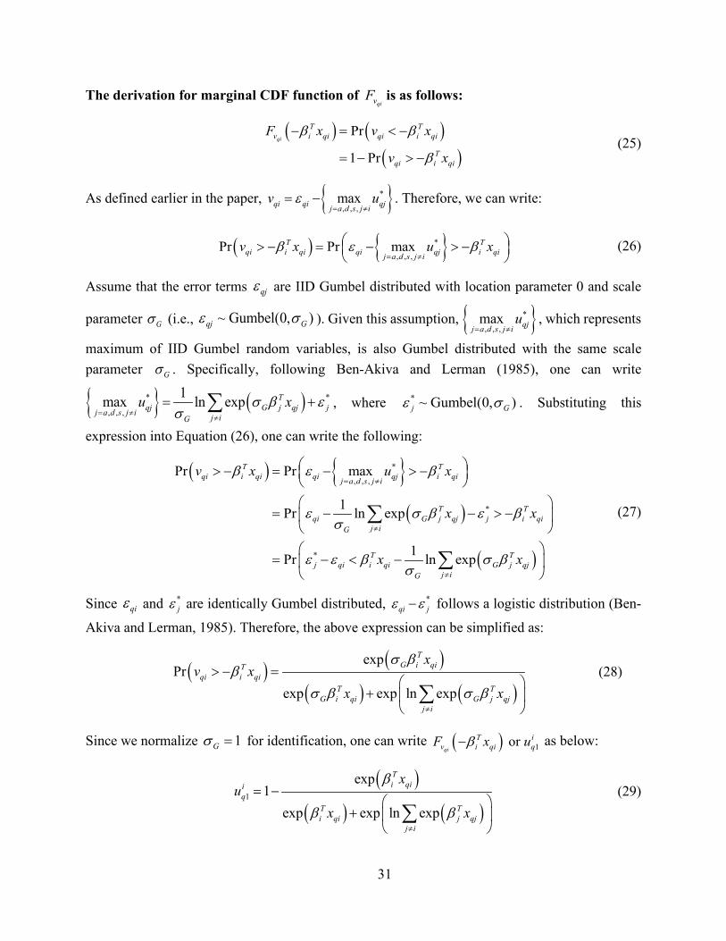
31
The derivation for marginal CDF function of qivF is as follows:
( ) ( )
( )Pr
1 Prqi
T Tv i qi qi i qi
Tqi i qi
F x v x
v x
β β
β
− = < −
= − > − (25)
As defined earlier in the paper, { }*
, , ,maxqi qi qjj a d s j i
v uε= ≠
= − . Therefore, we can write:
( ) { }*
, , ,Pr Pr maxT T
qi i qi qi qj i qij a d s j iv x u xβ ε β
= ≠
> − = − > −
(26)
Assume that the error terms qjε are IID Gumbel distributed with location parameter 0 and scale
parameter Gσ (i.e., ~ Gumbel(0, )qj Gε σ ). Given this assumption, { }*
, , ,max qjj a d s j i
u= ≠
, which represents
maximum of IID Gumbel random variables, is also Gumbel distributed with the same scale parameter Gσ . Specifically, following Ben-Akiva and Lerman (1985), one can write
{ } ( )* *
, , ,
1max ln exp Tqj G j qj jj a d s j i j iG
u xσ β εσ= ≠
≠
= +∑ , where * ~ Gumbel(0, )j Gε σ . Substituting this
expression into Equation (26), one can write the following:
( ) { }( )
( )
*
, , ,
*
*
Pr Pr max
1Pr ln exp
1Pr ln exp
T Tqi i qi qi qj i qij a d s j i
T Tqi G j qj j i qi
j iG
T Tj qi i qi G j qj
j iG
v x u x
x x
x x
β ε β
ε σ β ε βσ
ε ε β σ βσ
= ≠
≠
≠
> − = − > −
= − − > −
= − < −
∑
∑
(27)
Since qiε and *jε are identically Gumbel distributed, *
qi jε ε− follows a logistic distribution (Ben-
Akiva and Lerman, 1985). Therefore, the above expression can be simplified as:
( ) ( )( ) ( )
expPr
exp exp ln exp
TG i qiT
qi i qiT T
G i qi G j qjj i
xv x
x x
σ ββ
σ β σ β≠
> − =
+ ∑
(28)
Since we normalize 1Gσ = for identification, one can write ( ) 1 or qi
Tv i q
ii qxF uβ− as below:
( )
( ) ( )1
exp
exp exp ln e p1
x
Ti qi
T Ti qi j qj
j i
iqu
x
x x
β
β β≠
+
−
=
∑
(29)

32
References
Abou-Zeid, M., Kaysi, I., & Al-Naghi, H. (2011). Measuring aggressive driving behavior using a driving simulator: An exploratory study. In 3rd International Conference on Road Safety and Simulation.
Ahmed, K. I. (1999). Modeling drivers' acceleration and lane changing behavior. PhD Thesis, Massachusetts Institute of Technology.
Ahn, K., & Rakha, H. (2009). A field evaluation case study of the environmental and energy impacts of traffic calming. Transportation Research Part D: Transport and Environment, 14 (6), 411-424.
Ali, Y., Zheng, Z., Haque, M. M., & Wang, M. (2019). A game theory-based approach for modelling mandatory lane-changing behaviour in a connected environment. Transportation Research Part C: Emerging Technologies, 106, 220-242.
Asaithambi, G., Kanagaraj, V., & Toledo, T. (2016). Driving behaviors: Models and challenges for non-lane based mixed traffic. Transportation in Developing Economies, 2 (2), 19.
Bando, M., Hasebe, K., Nakayama, A., Shibata, A., & Sugiyama, Y. (1995). Dynamical model of traffic congestion and numerical simulation. Physical review E, 51 (2), 1035.
Ben-Akiva, M. E., & Lerman, S. R. (1985). Discrete choice analysis: theory and application to travel demand. MIT press.
Bexelius, S. (1968). An extended model for car-following. Transportation Research, 2 (1), 13-21. Bhat, C. R., & Eluru, N. (2009). A copula-based approach to accommodate residential self-selection effects in travel
behavior modeling. Transportation Research Part B: Methodological, 43 (7), 749-765. Brackstone, M., & McDonald, M. (1999). Car-following: a historical review. Transportation Research Part F: Traffic
Psychology and Behaviour, 2 (4), 181-196. Budhkar, A. K., & Maurya, A. K. (2017). Multiple-leader vehicle-following behavior in heterogeneous weak lane
discipline traffic. Transportation in Developing Economies, 3 (2), 20. Calvert, S. C., Schakel, W. J., & van Lint, J. W. C. (2020). A generic multi-scale framework for microscopic traffic
simulation part II–Anticipation Reliance as compensation mechanism for potential task overload. Transportation Research Part B: Methodological, 140, 42-63.
Cameron, A. C., Li, T., Trivedi, P. K., & Zimmer, D. M. (2004). Modelling the differences in counted outcomes using bivariate copula models with application to mismeasured counts. The Econometrics Journal, 7 (2), 566-584.
Chakroborty, P., Agrawal, S., & Vasishtha, K. (2004). Microscopic modeling of driver behavior in uninterrupted traffic flow. Journal of transportation engineering, 130 (4), 438-451.
Chakroborty, P., & Das, A. (2017). Principles of transportation engineering. PHI Learning Pvt. Ltd. Chakroborty, P., Maurya, A. K., & Vikram, D. (2019). Understanding and Modelling Disorderly Traffic Streams.
Journal of the Indian Institute of Science, 1-13. Chandler, R. E., Herman, R., & Montroll, E. W. (1958). Traffic dynamics: studies in car following. Operations
research, 6 (2), 165-184. Chen, J., Liu, R., Ngoduy, D., & Shi, Z. (2016). A new multi-anticipative car-following model with consideration of
the desired following distance. Nonlinear Dynamics, 85 (4), 2705-2717. Cho, H.-J., & Wu, Y.-T. (2004). Modeling and simulation of motorcycle traffic flow. In 2004 IEEE International
Conference on Systems, Man and Cybernetics. IEEE. Choudhury, C. F. (2007). Modeling driving decisions with latent plans. PhD Thesis, Massachusetts Institute of
Technology. Choudhury, C. F., & Islam, M. M. (2016). Modelling acceleration decisions in traffic streams with weak lane
discipline: A latent leader approach. Transportation Research Part C: Emerging Technologies, 67, 214-226. Das, S., & Maurya, A. K. (2018). Modelling of motorised two-wheelers: a review of the literature. Transport reviews,
38 (2), 209-231. Edie, L. C. (1961). Car-following and steady-state theory for noncongested traffic. Operations research, 9 (1), 66-76. Embrechts, P., McNeil, A., & Straumann, D. (2002). Correlation and dependence in risk management: properties and
pitfalls. Risk management: value at risk and beyond, 1, 176-223. Farhi, N., Haj-Salem, H., & Lebacque, J.-P. (2012). Multianticipative piecewise-linear car-following model.
Transportation Research Record: Journal of the Transportation Research Board, 100-109. Gartner, N. H., Messer, C. J., & Rathi, A. (2002). Traffic flow theory-A state-of-the-art report: revised monograph on
traffic flow theory.

33
Gazis, D. C., Herman, R., & Potts, R. B. (1959). Car-following theory of steady-state traffic flow. Operations research, 7 (4), 499-505.
Gazis, D. C., Herman, R., & Rothery, R. W. (1961). Nonlinear follow-the-leader models of traffic flow. Operations research, 9 (4), 545-567.
Ge, H. X., Dai, S. Q., Dong, L. Y., & Xue, Y. (2004). Stabilization effect of traffic flow in an extended car-following model based on an intelligent transportation system application. Physical review E, 70 (6), 066134.
Genest, C., & Favre, A.-C. (2007). Everything you always wanted to know about copula modeling but were afraid to ask. Journal of hydrologic engineering, 12 (4), 347-368.
Gunay, B. (2007). Car following theory with lateral discomfort. Transportation Research Part B: Methodological, 41 (7), 722-735.
HCM. (2000). Highway Capacity Manual. Transportation Research Board. Helly, W. (1959). Simulation of bottlenecks in single-lane traffic flow. In Proceedings of the Symposium on Traffic
Flow Theory, Research Laboratories, General Motors, New York. Herman, R., & Potts, R. B. (1959). Single lane traffic theory and experiment. Theory of Traffic Flow, 120-146. Hoogendoorn, S. P., & Ossen, S. (2006). Empirical analysis of two-leader car-following behavior. European journal
of transport and infrastructure research, 6 (3), 229-246. Hoogendoorn, S. P., Ossen, S., & Schreuder, M. (2006). Empirics of multianticipative car-following behavior.
Transportation Research Record, 1965 (1), 112-120. Hoque, M. S. (1994). The modelling of signalized intersections in developing countries. PhD Thesis, University of
Southampton, United Kingdom. Hossain, M., & McDonald, M. (1998). Modelling of traffic operations in urban networks of developing countries: a
computer aided simulation approach. Computers, environment and urban systems, 22 (5), 465-483. Hu, Y., Ma, T., & Chen, J. (2014). An extended multi-anticipative delay model of traffic flow. Communications in
nonlinear science and numerical simulation, 19 (9), 3128-3135. Jin, S., Wang, D.-h., Xu, C., & Huang, Z.-y. (2012). Staggered car-following induced by lateral separation effects in
traffic flow. Physics Letters A, 376 (3), 153-157. Jin, Y., Xu, M., Gao, Z., & Dynamics, N. (2011). KdV and kink-antikink solitons in an extended car-following model.
6 (1), 011018. Kanagaraj, V., Asaithambi, G., Toledo, T., & Tzu-Chang, L. (2015). Trajectory data and flow characteristics of mixed
traffic. Transportation Research Record: Journal of the Transportation Research Board, 2491 (1), 1-11. Kanagaraj, V., & Treiber, M. (2018). Self-driven particle model for mixed traffic and other disordered flows. Physica
A: Statistical Mechanics and its Applications, 509, 1-11. Koutsopoulos, H. N., & Farah, H. (2012). Latent class model for car following behavior. Transportation Research Part
B: Methodological, 46 (5), 563-578. Lajunen, T., & Parker, D. (2001). Are aggressive people aggressive drivers? A study of the relationship between self-
reported general aggressiveness, driver anger and aggressive driving. Accident Analysis & Prevention, 33 (2), 243-255.
Lan, L., & Chang, C. (2004). Motorcycle-following models of General Motors (GM) and adaptive neuro-fuzzy inference system. Transportation Planning Journal, 33 (3), 511-536.
Lee, T.-C., Polak, J. W., & Bell, M. G. (2009). New approach to modeling mixed traffic containing motorcycles in urban areas. Transportation Research Record, 2140 (1), 195-205.
Lenz, H., Wagner, C., & Sollacher, R. (1999). Multi-anticipative car-following model. The European Physical Journal B-Condensed Matter and Complex Systems, 7 (2), 331-335.
Li, L., Chen, X., & Li, Z. (2013). Asymmetric stochastic Tau Theory in car-following. Transportation Research Part F: Traffic Psychology and Behaviour, 18, 21-33.
Li, Y., Sun, D., Liu, W., Zhang, M., Zhao, M., Liao, X., & Tang, L. (2011). Modeling and simulation for microscopic traffic flow based on multiple headway, velocity and acceleration difference. Nonlinear Dynamics, 66 (1-2), 15-28.
Li, Z.-P., & Liu, Y.-C. (2006). Analysis of stability and density waves of traffic flow model in an ITS environment. The European Physical Journal B-Condensed Matter and Complex Systems, 53 (3), 367-374.
Lu, B., Ni, S., & Washburn, S. S. (2015). A support vector regression approach for investigating multianticipative driving behavior. Mathematical Problems in Engineering, 2015.
Mahapatra, G., Maurya, A. K., & Chakroborty, P. (2018). Parametric study of microscopic two-dimensional traffic flow models: A literature review. Canadian Journal of Civil Engineering, 45 (11), 909-921.
Maini, P. (2002). Development of a vehicle-following model (VEHFOL) and a heterogeneous traffic simulation model (HETSIM) for controlled intersections. PhD Thesis, University of Colorado at Denver, Colorado.

34
Mallikarjuna, C., & Rao, K. R. (2011). Heterogeneous traffic flow modelling: a complete methodology. Transportmetrica, 7 (5), 321-345.
Maurya, A. (2007). Development of a comprehensive microscopic model for simulation of large uninterrupted traffic streams without lane discipline. Indian Institute of Technology, Kanpur.
May, A., & Keller, H. E. (1967). Non-integer car-following models. Highway Research Record, 199 (1), 19-32. Munigety, C. R. (2018). A spring-mass-damper system dynamics-based driver-vehicle integrated model for
representing heterogeneous traffic. International Journal of Modern Physics B, 32 (11), 1850135. Munigety, C. R., & Mathew, T. V. (2016). Towards behavioral modeling of drivers in mixed traffic conditions.
Transportation in Developing Economies, 2 (1), 6. Nagatani, T. (1999). Stabilization and enhancement of traffic flow by the next-nearest-neighbor interaction. 60 (6),
6395. Ni, D. (2015). Traffic flow theory: Characteristics, experimental methods, and numerical techniques. Butterworth-
Heinemann. Ossen, S. J. L. (2008). Longitudinal driving behavior: theory and empirics. Oviedo-Trespalacios, O., Haque, M. M., King, M., & Washington, S. (2017). Effects of road infrastructure and traffic
complexity in speed adaptation behaviour of distracted drivers. Accident Analysis & Prevention, 101, 67-77. Ozaki, H. (1993). Reaction and anticipation in the car-following behavior. In Proceedings of 12th International
Symposium on Theory of Traffic Flow and Transportation. Panwai, S., & Dia, H. (2007). Neural agent car-following models. IEEE Transactions on Intelligent Transportation
Systems, 8 (1), 60-70. Park, B. B., & Won, J. (2006). Microscopic simulation model calibration and validation handbook. Virginia
Transportation Research Council. Paschalidis, E., Choudhury, C. F., & Hess, S. (2019). Combining driving simulator and physiological sensor data in a
latent variable model to incorporate the effect of stress in car-following behaviour. Analytic Methods in Accident Research, 22, 100089.
Peng, G., & Sun, D. (2010). A dynamical model of car-following with the consideration of the multiple information of preceding cars. Physics Letters A, 374 (15-16), 1694-1698.
Punzo, V., Borzacchiello, M. T., & Ciuffo, B. (2011). On the assessment of vehicle trajectory data accuracy and application to the Next Generation SIMulation (NGSIM) program data. Transportation Research Part C: Emerging Technologies, 19 (6), 1243-1262.
Ravishankar, K., & Mathew, T. V. (2011). Vehicle-type dependent car-following model for heterogeneous traffic conditions. Journal of transportation engineering, 137 (11), 775-781.
Saifuzzaman, M., & Zheng, Z. (2014). Incorporating human-factors in car-following models: a review of recent developments and research needs. Transportation Research Part C: Emerging Technologies, 48, 379-403.
Saifuzzaman, M., Zheng, Z., Haque, M. M., & Washington, S. (2015). Revisiting the Task–Capability Interface model for incorporating human factors into car-following models. Transportation Research Part B: Methodological, 82, 1-19.
Sarkar, N. C., Bhaskar, A., Zheng, Z., & Miska, M. P. (2020). Microscopic modelling of area-based heterogeneous traffic flow: Area selection and vehicle movement. Transportation Research Part C: Emerging Technologies, 111, 373-396.
Sayer, J. R., Mefford, M. L., & Huang, R. W. (2003). The effects of lead-vehicle size on driver following behavior: Is ignorance truly bliss? In Proceedings of the Second International Driving Symposium on Human Factors in Driver Assessment, Training and Vehicle Design.
Sharma, A., Ali, Y., Saifuzzaman, M., Zheng, Z., & Haque, M. M. (2017). Human factors in modelling mixed traffic of traditional, connected, and automated vehicles. In International Conference on Applied Human Factors and Ergonomics. Springer.
Sharma, A., Zheng, Z., & Bhaskar, A. (2018). A pattern recognition algorithm for assessing trajectory completeness. Transportation Research Part C: Emerging Technologies, 96, 432-457.
Sharma, A., Zheng, Z., Bhaskar, A., & Haque, M. M. (2019). Modelling car-following behaviour of connected vehicles with a focus on driver compliance. Transportation Research Part B: Methodological, 126, 256-279.
Siuhi, S. (2009). Parametric study of stimulus-response behavior incorporating vehicle heterogeneity in car-following models. PhD Thesis, University of Nevada, Las Vegas.
Sklar, A. (1973). Random variables, joint distribution functions, and copulas. Kybernetika, 9 (6), 449-460. Spissu, E., Pinjari, A. R., Pendyala, R. M., & Bhat, C. R. (2009). A copula-based joint multinomial discrete–
continuous model of vehicle type choice and miles of travel. Transportation, 36 (4), 403-422. Subramanian, H. (1996). Estimation of car-following models. PhD Thesis, Massachusetts Institute of Technology.

35
Tao, P., Hu, H., Gao, Z., Li, Z., Song, X., Xing, Y., Wei, F., & Duan, Y. (2015). An Improved General Motor Car-Following Model considering the Lateral Impact. Advances in Mechanical Engineering, 7 (2), 894589.
Tasca, L. (2000). A review of the literature on aggressive driving research. Ontario Advisory Group on Safe Driving Secretariat, Road User Safety Branch, Ontario Ministry of Transportation.
Toledo, T. (2003). Integrated Driving Behavior Modeling. PhD Thesis, Massachusetts Institute of Technology. Toledo, T. (2007). Driving behaviour: models and challenges. Transport reviews, 27 (1), 65-84. Treiber, M., Kesting, A., & Helbing, D. (2006). Delays, inaccuracies and anticipation in microscopic traffic models.
Physica A: Statistical Mechanics and its Applications, 360 (1), 71-88. Treiber, M., Kesting, A., & Helbing, D. (2007). Influence of reaction times and anticipation on stability of vehicular
traffic flow. Transportation Research Record, 1999 (1), 23-29. van Lint, J. c. C., & Calvert, S. C. (2018). A generic multi-level framework for microscopic traffic simulation-Theory
and an example case in modelling driver distraction. Transportation Research Part B: Methodological, 117, 63-86.
Wang, T., Gao, Z. Y., & Zhao, X. M. (2006). Multiple velocity difference model and its stability analysis. Acta Physica Sinica, 55 (2), 634.
Wilson, R., Berg, P., Hooper, S., & Lunt, G. (2004). Many-neighbour interaction and non-locality in traffic models. The European Physical Journal B-Condensed Matter and Complex Systems, 39 (3), 397-408.
Zhang, X. (2014). Empirical analysis of a generalized linear multianticipative car-following model in congested traffic conditions. Journal of transportation engineering, 140 (6), 04014018.
Zheng, Z. (2014). Recent developments and research needs in modeling lane changing. Transportation Research Part B: Methodological, 60, 16-32.
Zimmer, D. M., & Trivedi, P. K. (2006). Using trivariate copulas to model sample selection and treatment effects: application to family health care demand. Journal of Business & Economic Statistics, 24 (1), 63-76.