A DISCONTINUOUS GALERKIN METHOD TO SOLVE THE EEG …wolters/ChildBrainPapers/...A DISCONTINUOUS GALERKIN METHOD FOR EEG B139 to solve the underlying partial di erential equations in

SIAM J. SCI. COMPUT. c© 2017 Society for Industrial and Applied MathematicsVol. 39, No. 1, pp. B138–B164

A DISCONTINUOUS GALERKIN METHOD TO SOLVE THE EEGFORWARD PROBLEM USING THE SUBTRACTION APPROACH∗

CHRISTIAN ENGWER† , JOHANNES VORWERK‡ , JAKOB LUDEWIG§ ,

AND CARSTEN H. WOLTERS¶

Abstract. In order to perform electroencephalography (EEG) source reconstruction, i.e., tolocalize the sources underlying a measured EEG, the electric potential distribution at the electrodesgenerated by a dipolar current source in the brain has to be simulated, which is the so-called EEGforward problem. To solve it accurately, it is necessary to apply numerical methods that are ableto take the individual geometry and conductivity distribution of the subject’s head into account.In this context, the finite element (FE) method (FEM) has shown high numerical accuracy withthe possibility to model complex geometries and conductive features, e.g., white matter conductivityanisotropy. In this article, we introduce and analyze the application of a discontinuous Galerkin (DG)method, an FEM that includes features of the finite volume framework, to the EEG forward problem.The DG-FEM approach fulfills the conservation property of electric charge also in the discrete case,making it attractive for a variety of applications. Furthermore, as we show, this approach can alleviatemodeling inaccuracies that might occur in head geometries when using classical FE methods, e.g., so-called “skull leakage effects,” which may occur in areas where the thickness of the skull is in the rangeof the mesh resolution. Therefore, we derive a DG formulation of the FEM subtraction approachfor the EEG forward problem and present numerical results that highlight the advantageous featuresand the potential benefits of the proposed approach.

Key words. discontinuous Galerkin, finite element method, conservation properties, EEG,dipole, subtraction method, realistic head modeling

AMS subject classifications. 35J25, 35J75, 35Q90, 65N12, 65N30, 68U20, 92C50

DOI. 10.1137/15M1048392

1. Introduction. Electroencephalography (EEG) source reconstruction is nowa-days widely used in both research and clinical routine to investigate the activity of thehuman brain, as it is a noninvasive, easy to perform, and relatively cheap technique[29, 17]. To reconstruct the active brain areas from the electric potentials measuredat the head surface, it is necessary to simulate the electric potential generated by adipolar current source in the gray matter compartment of the brain, the so-called EEGforward problem. The achievable accuracy in solving the forward problem stronglydepends on a realistic modeling of shape and conductive features of the volume con-ductor, i.e., the human head. Therefore, it is necessary to apply numerical methods

∗Submitted to the journal’s Computational Methods in Science and Engineering section Novem-ber 16, 2015; accepted for publication (in revised form) November 9, 2016; published electronicallyFebruary 23, 2017.

http://www.siam.org/journals/sisc/39-1/M104839.htmlFunding: This work was partially supported by the Deutsche Forschungsgemeinschaft (DFG),

project WO1425/7-1, the Priority Program 1665 of the Deutsche Forschungsgemeinschaft (DFG)(WO1425/5-1, 5-2), the Cluster of Excellence 1003 of the Deutsche Forschungsgemeinschaft (DFGEXC 1003 Cells in Motion), and by EU project ChildBrain (Marie Curie Innovative Training Net-works, grant agreement 641652).†Institute for Computational and Applied Mathematics, University of Munster, Einsteinstraße

62, 48149 Munster, Germany ([email protected]).‡Institute for Biomagnetism and Biosignalanalysis, University of Munster, Malmedyweg 15, 48149

Munster, Germany ([email protected]).§Cluster of Excellence EXC 1003, Cells in Motion CiM Munster, Germany (jakobludewig@

gmx.net).¶Scientific Computing and Imaging (SCI) Institute, University of Utah, 72 S Central Campus

Drive, Salt Lake City, UT 84112 ([email protected]).

B138

http://www.siam.org/journals/sisc/39-1/M104839.html

mailto:[email protected]





A DISCONTINUOUS GALERKIN METHOD FOR EEG B139

to solve the underlying partial differential equations in realistic geometries, since an-alytical solutions exist for only a few special cases, e.g., nested shells [21]. Differentnumerical methods have been proposed to solve this problem, e.g., boundary ele-ment methods [33, 1, 28, 45], finite volume methods [20], finite difference methods[55, 49, 32], or finite element FE methods (FEMs) [13, 31, 41, 25, 37, 35]. FEMswere shown to achieve high numerical accuracies [25, 52] and offer the importantpossibility of modeling complex geometries and also anisotropic conductivities, withonly a weak influence on the computational effort [51]. The computational burden ofusing FE methods to solve the EEG forward problem could be clearly reduced by theintroduction of transfer matrices and fast solver methods [54, 26, 58].

One of the main tasks in applying FE methods to solve the EEG forward problemis to deal with the strong singularity introduced by the source model of a currentdipole. Therefore, different approaches to solve the EEG forward problem using theFEM have been proposed, e.g., the Saint-Venant [47, 43, 18, 52], the partial integration[61, 54, 48, 52], the Whitney or Raviart–Thomas [46, 35], or the subtraction approach[13, 31, 41, 60, 25, 52]. All these approaches rely on a continuous Galerkin (CG) FEM(CG-FEM) formulation, also called Lagrange or conforming FEM, i.e., the resultingsolution for the electric potential is continuous.

The use of tetrahedral [31, 25, 51] as well as that of hexahedral [41, 39, 7, 6] mesheshas been proposed for solving the EEG forward problem with the FEM. Tetrahedralmeshes can be generated by constrained Delaunay tetrahedralizations (CDT) fromgiven tissue surface representations [25, 51]. This approach has the advantage thatsmooth tissue surfaces are well represented in the model. On the other hand, thegeneration of such models is difficult in practice and might cause unrealistic modelfeatures, e.g., holes in tissue compartments such as the foramen magnum and the opticcanals in the skull are often artificially closed to allow CDT meshing. Furthermore,CDT modeling necessitates the generation of nested, nonintersection, and nontouch-ing surfaces. However, in reality, surfaces might touch, for example, the inner skulland outer brain surface. Hexahedral models do not suffer from such limitations, canbe easily generated from voxel-based magnetic resonance imaging (MRI) data, andare more and more frequently used in source analysis applications [39, 7, 6]. Thispaper therefore focuses on the application of FE methods with hexahedral meshes.However, the application of the CG-FEM with hexahedral meshes has the disadvan-tage that the representation of thin tissue structures in combination with insufficientmesh resolutions might result in geometry approximation errors. It has been shown,e.g., in [44], that the combination of thin skull structures and insufficient hexahe-dral mesh resolutions might result in so-called skull leakages in areas where scalp andCerebrospinal Fluid (CSF) elements are erroneously connected via single skull verticesor edges, as illustrated in Figure 1. Such leakages can lead to significantly inaccu-rate results when using vertex-based methods like, e.g., the CG-FEM, and might beone of the main reasons why in a recent head modeling comparison study for EEGsource analysis in presurgical epilepsy diagnosis, the use of the CG-FEM with a four-layer hexahedral head model with a resolution of 2 mm did not lead to better resultsthan those for simpler head models, i.e., a three-layer local sphere and a three-layerboundary element head model [14].

In this paper, we derive the mathematical equations underlying the forward prob-lem of EEG and introduce its solution using the subtraction approach. After a shortexplanation of the strengths and weaknesses of this approach, we propose and evalu-ate a new formulation of the subtraction approach on the basis of the discontinuousGalerkin (DG) FEM (DG-FEM). We then show that, although the CG-FEM and

B140 ENGWER, VORWERK, LUDEWIG, AND WOLTERS

DG-FEM achieve similar numerical accuracies in multilayer sphere validation studieswith high mesh resolutions, the DG-FEM mitigates the problem of skull leakages inthe case of lower mesh resolutions. The results of the sphere studies are complementedand underlined by the results obtained in a realistic six-compartment head model.

2. Theory.

2.1. The forward problem. The partial differential equation underlying theEEG forward problem can be derived by introducing the quasi-static approximationof Maxwell’s equations [29, 17]. When relating the electric field to a scalar potential,E = −∇u, and splitting up the current density J into a term f , which describes thecurrent source, and a return current, or flux, −σ∇u with σ(x) being the conductivitydistribution in the head domain, we obtain a Poisson equation

−∇ · (σ∇u) = f in Ω,(2.1a)

σ∂nu = 0 on ∂Ω,(2.1b)

where Ω denotes the head domain, which is assumed to be open and connected, and∂Ω its boundary. We have homogeneous Neumann boundary conditions here, sincewe assume a conductivity σ(x) = 0 for all x /∈ Ω.

2.2. The subtraction approach. We briefly derive the classical subtraction FEapproach as presented in [60, 25]. We assume the commonly used point-like dipolesource at position y with moment p, fy(x) = ∇ · (pδy(x)). This choice complicatesthe further mathematical treatment, as the right-hand side is not square integrable inthis case. However, when assuming that there exists a nonempty open neighborhoodΩ∞ of the source position y with constant isotropic conductivity σ∞, we can split thepotential u and the conductivity σ into two parts,

u = u∞ + ucorr,(2.2a)

σ = σ∞ + σcorr.(2.2b)

u∞ is the potential in an unbounded, homogeneous conductor and can be calculated

analytically: u∞(x) = 14πσ∞

〈p,x−y〉|x−y|3 . The more general case of anisotropic conductiv-

ities can be treated too [60, 25], but is not especially derived here.Inserting the decomposition of u into (2.1) and subtracting the homogeneous

solution, again results in a Poisson equation for the searched correction potentialucorr:

−∇ · (σ∇ucorr) = ∇ · (σcorr∇u∞) in Ω,(2.3a)

σ∂nucorr = −σ∂nu∞ on ∂Ω.(2.3b)

To solve this problem numerically, [25] proposes a conforming first-order FEM: Finducorr ∈ Vh ⊂ H1 such that it fulfills the weak formulation

(2.4)

∫Ω

σ∇ucorr · ∇vdx = −∫Ω

σcorr∇u∞ · ∇vdx−∫∂Ω

σ∞∂nu∞vds.

The weak form can be heuristically derived by multiplication with a test functionv ∈ Vh and subsequent partial integration. Reorganization of some terms and applyingthe identity (2.2b) yields the proposed form in (2.4). The subtraction approach istheoretically well understood. The existence of a solution as well as the uniquenessand convergence of this solution are examined in [60, 25].


Fig. 1. Sketch of segmentation that might lead to leakage effects (left). The yellow line showsthe inner skull surface, the red line the original outer skull surface, the blue line the corrected outerskull surface. Where the red and the blue line overlap, only the blue line is visible. In the magnifieddetail, the scalp and CSF show two erroneous connections via single vertices or edges (right subfigure,where the red and the yellow line touch each other). Such a segmentation can lead to significantlyinaccurate results when using vertex-based methods such as, for example, the CG-FEM.

2.3. Skull leakage effects. As discussed in the introduction, hexahedral meshesare frequently used in practical applications of FEM-based EEG/magnetoencephalo-graphy source analysis, due to the clearly simplified creation process in comparisonto CDT meshes. A pitfall that has to be taken into account in this scenario is leakageeffects, especially in the thin skull compartment. If the segmentation resolution, i.e.,the resolution of the discrete approximation of the geometry, is coarse compared tothe thickness of the skull, segmentation artifacts as illustrated in Figure 1 (yellow andred lines) occur. When directly generating a hexahedral mesh from this segmentation,elements belonging to the highly conductive compartments interior to the skull, i.e.,most often the CSF, and to the skin compartment are now connected via a sharedvertex or edge, although they are physically separated in reality. When using such amesh e.g., for, the CG-FEM with Lagrange ansatz functions, these artifacts lead toskull leakage, as sketched in Figure 2. As a consequence of the vertex-based ansatzfunctions, the shared vertices have inadequately high entries in the stiffness matrix,which result in current leakage “through” these vertices.

This effect remains unchanged even when (globally or locally) refining the reso-lution of the mesh. An increase of the image—and thereby also the segmentation—resolution might eliminate this effect, but is usually not possible. Instead, this problemmight be circumvented by artificially increasing the thickness of the skull segmentationin these areas (blue line in Figure 1). However, this workaround might, again, lead toinaccuracies in the EEG forward computation due to the now too thick representationof the skull compartment.

In the following section, we derive a DG formulation for the subtraction FEapproach. This formulation has the advantage that it is locally charge preserving andcontrols the current flow through element faces, thereby preventing possible leakageeffects; see illustration in Figure 2.

2.4. A DG formulation. Preserving fundamental physical properties is veryimportant in order to obtain reliable simulation results. As discussed in the previoussection, a correct approximation of the electric current is crucial for reliable simulation


CG-FEM DG-FEM

Fig. 2. CG-FEM simulations lead to an overestimated electric current at degenerated verticesof the skull. This effect is due to the vertex-based discretization, which considers only the poten-tial, but not the electric current. The DG-FEM is based on a current reconstruction through cellfaces. Therefore, these methods do not overestimate the electric current, even in the presence ofsegmentation artifacts.

results. Continuity of the normal component of the current directly implies conserva-tion of charge.

The DG method allows us to construct formulations that preserve such conser-vation properties also in the discretized space. We first discuss which quantities topreserve when using the subtraction approach for the continuous problem and thenintroduce a DG formulation.

2.4.1. Conservation properties. A fundamental physical property is the con-servation of charge:

(2.5)

∫∂K

σ∇u · ~n ds =

∫K

fydx

for any control volume K ⊆ Ω. Following the subtraction approach, we split thecurrent σ∇u = (σ∞ + σcorr)∇(u∞ + ucorr). Rearrangement then yields∫

∂K

σ∇ucorr · ~n ds = −∫∂K

σcorr∇u∞ · ~n dx−∫∂K

σ∞∇u∞ · ~n ds+

∫K

fydx

︸︷︷︸≡0

.

Applying Gauss’s theorem to the right-hand side, we obtain a conservation propertyfor the correction potential,

(2.6)

∫∂K

σ∇ucorr︸︷︷︸~jcorr

·~n ds =

∫K

−∇ · σcorr∇u∞︸︷︷︸fcorr

dx ,

which basically states that the correction potential ucorr causes a flux ~jcorr; thecharge corresponding to this flux is a conserved property with source term f corr =∇ · σcorr∇u∞.

For FE methods this property carries over to the discrete solution, if the testspace contains the characteristic function, which is one on K and zero everywhereelse. In general, a conforming discretization does not guarantee this property.

Conservation of charge also holds for u∞ in the case of a homogeneous volumeconductor (with conductivity σ∞ in our case). Thus, the normal components of both


y

x

γ

Kr

Kl

K

Fig. 3. Interface γ splits K into two parts.

the electrical flux σ∇u and σ∞∇u∞ are continuous. Rewriting ~j in terms of σcorr,σ∞, ucorr, and u∞ we can show that the normal component of σ∇ucorr + σcorr∇u∞is also continuous.

Definition 2.1. We consider an arbitrary interface γ, which separates the con-trol volume K into two patches Kl and Kr (see Figure 3). Following [3], we introducethe jump of a scalar function u or a vector-valued function ~v along γ as

JuKγ := u|∂Kl~nKl

+ u|∂Kr~nKr

,(2.7a)

J~vKγ := ~v|∂Kl· ~nKl

+ ~v|∂Kr· ~nKr

.(2.7b)

Note that this is consistent with the following definition,

JuKγ(x) =

(lim

x′→x in Kl

u(x′)− limx′→x in Kr

u(x′)

)~nγ ,

and correspondingly for the vector-valued function ~v. Note further that the jump of ascalar function is vector valued, while the jump of a vector-valued function is scalar.

Lemma 2.2. Given a potential u with a flux σ∇u with with continuous normalcomponent along any surface, the normal component of σ∇ucorr + σcorr∇u∞ for thesubtraction approach is also continuous.

Proof. We consider an arbitrary interface γ. At each point x along γ the normalcomponents of the fluxes, σ∇u ·~nγ and σ∞∇u∞ ·~nγ , are continuous. Thus, the jumpvanishes for them and we obtain

(2.8) Jσ∇uKγ = 0 = Jσ∞∇u∞Kγ .

Rewriting Jσ∇uKγ in terms of σcorr, σ∞, ucorr, and u∞, we obtain

Jσ∞∇ucorrKγ + Jσcorr∇ucorrKγ + Jσcorr∇u∞Kγ = 0

⇔ Jσ∇ucorrKγ = −Jσcorr∇u∞Kγ⇔ Jσ∇ucorr + σcorr∇u∞Kγ = 0.(2.9)

As this property holds for any control volume, the normal component of the combinedflux σ∇ucorr + σcorr∇u∞ is also continuous for any interface γ.


Note that this also implies the identity

(2.10) Jσ∇ucorrKγ = −Jσcorr∇u∞Kγ

for any interface γ, which is later needed to derive the weak form (2.24a) from (2.20)and (2.21).

2.4.2. A weak formulation. An alternative to the conforming discretizationsketched in section 2.2 is to use more general trial and test spaces. We suggest employ-ing a symmetric DG discretization. The standard derivation of the DG formulationdoes not apply immediately, as the intrinsic conservation property for ucorr differs fromthe conservation property of the classical Poisson problem. In the following section,we will briefly describe the most important steps in the construction of a symmetricinterior penalty Galerkin (SIPG) DG formulation for the subtraction approach. Forfurther details on DG methods, we refer to [3] or the book of DiPietro and Ern [22].We start with the usual definitions.

Definition 2.3 (triangulation Th(Ω)). Let Th(Ω) be a finite collection of disjointand open subsets forming a partition of Ω. The subscript h corresponds to the meshwidth h := max diam(E) | E ∈ Th. Furthermore, the triangulation induces the in-ternal skeleton

(2.11) Γint := γe,f = ∂Ee ∩ ∂Ef | Ee, Ef ∈ Th , Ee 6= Ef , |γe,f | > 0

and the skeleton Γ := Γint ∪ ∂Ω.

Definition 2.4 (broken polynomial spaces). Broken polynomial spaces are de-fined as piecewise polynomial spaces on the partition Th(Ω) as

(2.12) V kh :=v ∈ L2(Ω) : v|E ∈ P k(E)

,

where P k denotes the space of polynomial functions of degree k. They describe func-tions that exhibit elementwise polynomial behavior but may be discontinuous acrosselement interfaces.

Since the elements of V kh may admit discontinuities across element boundaries,the gradient of a function v ∈ V kh is not defined everywhere on Ω. To account for this,we introduce the broken gradient operator.

Definition 2.5 (broken gradient operator). The broken gradient ∇h : V kh →[Lk(Ω)]d is defined such that, for all v ∈ V kh

(2.13) (∇hv) |E = ∇(v|E) for all E ∈ Th(Ω).

Definition 2.6 (jump and average). Using the Definition 2.1 we introduce theabbreviated notation of the jump

JxKe,f := JxKγe,f

of a piecewise continuous function x on the interface γe,f between two adjacent ele-ments Ee, Ef ∈ Th. We further define the average operator

xe,f := ωe,fx|∂Ee+ ωf,ex|∂Ef

.(2.14)


The weights ωe,f and ωf,e can be chosen to be the arithmetic mean, but for the caseof heterogeneous conductivities, [23] has shown that a conductivity-dependent choiceis optimal:

ωe,f :=σf

σf + σeand ωf,e :=

σeσe + σf

.(2.15)

We further introduce the average operator with switched weights

x∗e,f := ωf,ex|∂Ee+ ωe,fx|∂Ef

,(2.16)

and obtain the following multiplicative property:

JxyKe,f = JxKe,fy∗e,f + xe,f JyKe,f .(2.17)

Using a Galerkin approach, we seek for a solution ucorrh ∈ V kh , which fulfills (2.3)

in a weak sense. We start the derivation by testing with a test function vh ∈ V kh :

(2.18) −∫Ω

∇ · σ∇ucorrh vh dx =

∫Ω

∇ · σcorr∇u∞vh dx .

On each E ∈ Th(Ω), we apply integration by parts. Element boundaries are splitinto the domain boundary and all internal edges. The electric current σ∇ucorr

h · ~nthrough the boundary is given by the inhomogeneous Neumann boundary conditions(2.3b). For the left-hand side, we obtain

lhs =−∫Ω

∇ · σ∇ucorrh vh dx

=

∫Ω

σ∇hucorrh · ∇hvh dx+

∫∂Ω

σ∇u∞ · ~n vh ds−∫

Γint

Jσ∇hucorrh vhK ds,

(2.19)

and, with the multiplicative property (2.17) follows

lhs =

∫Ω

σ∇hucorrh · ∇hvh dx+

∫∂Ω

σ∇u∞ · ~n vh︸︷︷︸term †

ds

−∫

Γint

Jσ∇hucorrh K︸︷︷︸

term ‡

vh∗ + σ∇hucorrh JvhK ds .

(2.20)

Applying the same relations for the right-hand side, we obtain

rhs = −∫Ω

σcorr∇u∞ · ∇hvh dx+

∫∂Ω

σcorr∇u∞ · ~n vh︸︷︷︸term †

ds

+

∫Γint

Jσcorr∇u∞K︸︷︷︸term ‡

vh∗ + σcorr∇u∞JvhK ds .

(2.21)

Summing up the boundary integrals (2.20)† and (2.21)† yields a remaining term−σ∞∇u∞ ·~n vh on the right-hand side. As discussed in section 2.4.1, the conservationproperties also imply that the normal component of σ∇ucorr+σcorr∇u∞ is continuous;see (2.9). For the discrete solution, we require the same conservation property; thusthe jump term (2.20)‡ equals −Jσcorr∇u∞K and cancels out with term (2.21)‡.


To gain adjoint consistency, we symmetrize the operator and add the additionalterm

(2.22) asym(ucorrh , vh) := −

∫Γint

σ∇hvhJucorrh K ds .

To guarantee coercivity, the left-hand side is supplemented with the penalty term

J(ucorrh , vh) = η

∫Γint

σγhγ

Jucorrh KJvhK ds ,(2.23)

where hγ and σγ denote local definitions of the mesh width and the electric conduc-tivity on an edge γ, respectively. In our particular case, we choose hγ according to[27] and σγ as the harmonic average of the conductivities of the adjacent elements[23]:

hγe,f =min(|Ee|, |Ef |)

|γe,f |and σγe,f :=

2σeσfσe + σf

.

The penalty parameter η has to be chosen large enough to ensure coercivity.This derivation yields the SIPG formulation [56, 38] or for weighted averages the

symmetric weighted interior penalty Galerkin method [23]:Find ucorr

h ∈ Vh such that

a(ucorrh , vh) + J(ucorr

h , vh) = l(vh) for all vh ∈ Vh(2.24a)

with

a(ucorrh , vh) = a(ucorr

h , vh) + asym(ucorrh , vh)

=

∫Ω

σ∇hucorrh · ∇hvh dx−

∫Γint

σ∇hucorrh JvhK + σ∇hvhJucorr

h K ds ,(2.24b)

J(ucorrh , vh) = η

∫Γint

σγhγ

Jucorrh KJvhK ds ,

(2.24c)

l(vh) =−∫Ω

σcorr∇u∞ · ∇hvh dx

+

∫Γint

σcorr∇u∞JvhK ds−∫∂Ω

σ∞∂nu∞vh ds .(2.24d)

Given the correction potential ucorrh , the full potential uh can be reconstructed as

uh = ucorrh + u∞.

Remark 2.7 (discrete properties). As a(ucorrh , vh) and J(ucorr

h , vh) are the sameoperators as in [23], the following properties follow immediately: The proposed SIPGdiscretization (2.24) is consistent and adjoint consistent with the strong problem (2.3),and for a sufficiently large constant η > 0 it has a unique solution.

Remark 2.8 (conservation property). Furthermore, for K ⊆ Th(Ω), (2.24) fulfillsa discrete conservation property∫

∂K

σ∇hucorrh − η σγ

hγJucorrh K︸︷︷︸

~jcorrh

ds =

∫K

−∇σcorr∇u∞︸︷︷︸fcorr

ds


Table 1Conductive compartments (from inside to outside).

Compartment Outer radius Conductivity

Brain 78 mm 0.33 S/m

CSF 80 mm 1.79 S/m

Skull 86 mm 0.01 S/m

Skin 92 mm 0.43 S/m

with the discrete flux ~jcorrh . For h→ 0, the jump Jucorr

h K vanishes and the discrete flux~jcorrh converges to the flux ~jcorr as defined in (2.6).

3. Methods.

3.1. Implementation and parameter settings. We implemented the DG-FEM subtraction approach in the DUNE framework [9, 8] using the DUNE PDELabtoolbox [12]. For reasons of comparison, we also implemented the CG-FEM subtrac-tion approach in the same framework. We use linear ansatz functions for both the DG(i.e., k = 1 in (2.12)) and CG approaches throughout this study. On a given triangu-lation Th, we choose basis functions φih, i ∈ [0, Nh), with local support, where Nhdenotes the number of unknowns. The penalty parameter η was chosen to be η = 0.39.For the CG simulations, a Lagrange basis with the usual hat functions is employed,whereas for the DG case, elementwise L2-orthonormal functions are chosen. In thissetup (k = 1, hexahedral mesh), we have eight unknowns per mesh cell for the DGapproach, i.e., Nh = 8 × #cells, and one unknown per vertex for the CG approach,i.e., Nh = #vertices. Evaluating the bilinear forms a(·, ·), J(·, ·), and the right-handside l(·) leads to a linear system A · x = b, where x ∈ RNh denotes the coefficientvector, and the approximated solution of (2.24) is ucorrh =

∑i xiφ

ih. Furthermore,

A ∈ RNh×Nh is the matrix representation of the bilinear operator a+ J and b ∈ RNh

the right-hand-side vector:

Aij = a(φjh, φih) + J(φjh, φ

ih) i, j ∈ [0, Nh),

bi = l(φih) i ∈ [0, Nh) .

The resulting matrix A has a sparse block structure with small dense blocks, in ourcase, of dimension 8 × 8. The outer structure is similar to that of a finite volumediscretization, i.e., rows corresponding to each grid cell and one off-diagonal entryfor each cell neighbor. By now, a range of efficient solvers for DG discretizations isavailable, using multigrid [10] or domain decomposition methods [2]. The computa-tion/solving times for the CG-FEM and DG-FEM for realistic six-layer head modelsand a realistic EEG sensor configuration are compared in the results section.

3.2. Volume conductor models. To validate and compare the accuracy ofthese numerical schemes, we used four-layer sphere volume conductor models, wherean analytical solution exists and can be used as a reference [21]. For the four sphericalcompartments, representing brain, CSF, skull, and skin, we chose radii and conduc-tivities as shown in Table 1. As discussed in the introduction and in 2.3, we usedhexahedral meshes in our study. To be able to distinguish between numerical andgeometrie errors, i.e., errors due to the discrete approximation of the continuous PDEand errors due to an inaccurate representation of the geometry, respectively, we con-structed a variety of head models with different segmentation resolutions (1 mm,


seg 1 res 1 seg 2 res 2 seg 4 res 4

Fig. 4. Visualization of models seg 1 res 1, seg 2 res 2, and seg 4 res 4 (from left to right), cutin the x-plane at the origin; coloring is brain—red, CSF—yellow, skull—green, skin—blue.

Table 2Model properties (from left to right): segmentation resolution (Seg.), mesh resolution (h), num-

ber of nodes, number of elements.

Seg. h #nodes #elements

seg 1 res 1 1 mm 1 mm 3,342,701 3,262,312

seg 2 res 1 2 mm 1 mm 3,343,801 3,263,232

seg 2 res 2 2 mm 2 mm 428,185 407,907

seg 4 res 1 4 mm 1 mm 3,351,081 3,270,656

seg 4 res 2 4 mm 2 mm 429,077 408,832

seg 4 res 4 4 mm 4 mm 56,235 51,104

6CI hex 1mm 1 mm 1 mm 3,965,968 3,871,029

6CI hex 2mm 2 mm 2 mm 508,412 484,532

6CI tet hr - - 2,242,186 14,223,508

Table 3Model parameters.

Out. skull rad. #leaks

seg 2 res 2 r82 82 mm 10,080

seg 2 res 2 r84 83 mm 1,344

seg 2 res 2 r84 84 mm 0

2 mm, and 4 mm) and for each of these we again used different mesh resolutions(1 mm, 2 mm, and 4 mm). Figure 4 visualizes a subset of the used models and thedetails of these head models are listed in Table 2.

To further evaluate the sensitivity of the different numerical methods to leakageeffects, we intentionally generated spherical models with skull leakages. Therefore,we chose the model seg 2 res 2 and reduced the radius of the outer skull boundaryto 82 mm, 83 mm, and 84 mm, resulting in skull thicknesses of 2 mm, 3 mm, and 4mm, respectively. This way, we were able to generate a leakage scenario similar tothe one presented in Figure 1, while preserving the advantage of a spherical solutionthat can be used for error evaluations. Table 3 indicates the number of leaks for eachmodel, i.e., the number of vertices belonging to both an element labeled as skin andan element labeled as CSF or brain.


3.3. Sources. Since the numerical accuracy depends on the local mesh structureand the source eccentricity, we used 10 source eccentricities and, for each eccentricity,randomly distributed 10 sources. Thereby, the variability of the numerical accuracycan be captured for each eccentricity. We evaluated the accuracy for both radial andtangential dipole directions; however, we present the results only for radial directionshere. The results for dipoles with tangential direction are very similar to these withslightly lower errors than for radial dipoles.

To make the effect of skull leakage more accessible, we additionally generatedvisualizations of the current for one dipole fixed at position (1, 47, 47), which corre-sponds to an element center, and fixed direction (0, 1, 1) for both the CG-FEM andDG-FEM and for all three models with reduced skull thickness as shown in Table 3.We visualized a cut through the x-plane at the dipole position and chose to visu-alize both the direction and strength of the electric flux for each numerical methodand model (Figure 9). Furthermore, the relative change in strength and the fluxdifference between the numerical methods, described by the metrics lnMAG~j,loc and

totDIFF~j,loc as defined in the next section, were visualized for each model (Figure 10).

3.4. Error metrics. To achieve a result that purely represents the numericaland segmentation accuracy and is independent of the chosen sensor configuration,we evaluated the solutions on the whole outer layer. We use two error measures todistinguish between topography and magnitude errors, the relative difference measure(RDM),

RDM(uh, u) =

∥∥∥∥ uh‖uh‖2

− u

‖u‖2

∥∥∥∥2

,(3.1)

and the logarithmic magnitude (lnMAG) error,

lnMAG(uh, u) = ln

(‖uh‖2‖u‖2

).(3.2)

Besides presenting the mean RDM and lnMAG errors over all sources at a certaineccentricity (see, e.g., left subfigures in Figure 6), we also present results in separateboxplots (see, e.g., right subfigures in Figure 6). The boxplots show maximum andminimum error over all source positions at a certain eccentricity, indicated by upperand lower error bars. This allows us to display the overall variability of the error. Fur-thermore, the boxplots show the upper and lower quartiles. The interquartile range ismarked by a box; a black dash shows the median. Henceforth, the interquartile rangewill also be denoted as spread. Note the different presentation of source eccentricityon the x-axes in the left and right subfigures.

To evaluate the local changes of the current, we furthermore visualize for eachmesh element E the logarithm of the local change in current magnitude

(3.3) lnMAG~j,loc (E) = ln

(‖~jh,CG(xE)‖2‖~jh,DG(xE)‖2

),

and the total local current difference

(3.4) totDIFF~j,loc (E) = ~jh,CG(xE)−~jh,DG(xE),

where xE denotes the centroid of mesh element E (see Figure 10).


Fig. 5. Visualization of realistic six-compartment hexahedral 6CI hex 2mm, h = 2mm, (left)and high-resolution reference head model 6CI tet hr (right).

We can exploit that, due to the relation ln(1 + x) ≈ x for small ‖x‖, we havelnMAG ≈ ‖uh‖2/‖u‖2−1 for small deviations. In consequence, 100 ·lnMAG is aboutthe change of the magnitude in percent. The same approximations are valid for thelnMAG~j,loc .

3.5. Realistic head model. To complete the numerical evaluations, the differ-ences between the CG-FEM and DG-FEM were evaluated in a more realistic scenario.Based on MRI recordings, a segmentation considering six tissue compartments (whitematter, gray matter, cerebrospinal fluid, skull compacta, skull spongiosa, and skin)that includes realistic skull openings such as the foramen magnum and the opticnerve canal was generated. Based on this segmentation, three realistic head modelswere generated. Two hexahedral head models with mesh resolutions of 1 mm and2 mm, 6CI hex 1mm and 6CI hex 2mm, were generated, resulting in 3,965,968 ver-tices and 3,871,029 elements, and 508,412 vertices and 484,532 elements, respectively(Figure 5). For both models, the segmentation resolution is identical to the meshresolution. As the model with a mesh width of 2 mm was not corrected for leakages,1,164 vertices belonging to both CSF and skin elements were found. These leakageswere mainly located at the temporal bone. To calculate reference solutions, a high-resolution tetrahedral head model with 2,242,186 vertices and 14,223,508 elements,6CI tet hr, was generated. For further details of this model and of the used segmenta-tion, please refer to [51, 50]. The conductivities were chosen according to [51]. 4,724source positions were placed in the gray matter with a normal constraint, and thosethat were not fully contained in the gray matter compartment, i.e., where the sourcewas placed in an element at a compartment boundary, were excluded. As a result,4,482 source positions remained for the 1-mm model and 4,430 source positions for the2-mm model. An 80-channel realistic EEG cap was chosen as the sensor configuration.For both the CG-FEM and DG-FEM, solutions in the 1-mm and 2-mm hexahedralhead model were computed and the RDM and lnMAG are evaluated in comparisonto the solution of the CG-FEM calculated using the tetrahedral head model.

The computations were performed on a Linux-PC with an Intel Xeon E5-2698v3 CPU (2.30 GHz). The computation times for the CG-FEM and DG-FEM inthe models 6CI hex 1mm and 6CI hex 2mm were evaluated in the results section.Though an optimal speedup through parallelization can be achieved for both the


0

0.1

0.2

0.3

0.4

0.5

0.6

0 0.1 0.2 0.3 0.4 0.5 0.6 0.7 0.8 0.9 1

RD

M

Eccentricity

seg_1_res_1

seg_2_res_1

seg_2_res_2

seg_4_res_1

seg_4_res_2

seg_4_res_4

0

0.2

0.4

0.6

0.8

1

1.2

0.010 0.502 0.748 0.871 0.933 0.964 0.979 0.987 0.991 0.993

RD

M

Eccentricity

seg_1_res_1

seg_2_res_1

seg_2_res_2

seg_4_res_1

seg_4_res_2

seg_4_res_4

0

0.05

0.1

0.15

0.2

0.25

0.3

0.35

0.4

0.45

0 0.1 0.2 0.3 0.4 0.5 0.6 0.7 0.8 0.9 1

lnM

AG

Eccentricity

seg_1_res_1

seg_2_res_1

seg_2_res_2

seg_4_res_1

seg_4_res_2

seg_4_res_4

-0.4

-0.2

0

0.2

0.4

0.6

0.8

1

0.010 0.502 0.748 0.871 0.933 0.964 0.979 0.987 0.991 0.993

lnM

AG

Eccentricity

seg_1_res_1

seg_2_res_1

seg_2_res_2

seg_4_res_1

seg_4_res_2

seg_4_res_4

Fig. 6. Convergence for the DG-FEM with increasing mesh and/or segmentation resolution.Results of radial dipole computations. Visualized are the mean error (left column) and boxplots(right column) of the RDM (top row) and lnMAG (bottom row). Dipole positions that are outsidethe brain compartment in the discretized models are marked as dots. Note the different scaling of thex-axes. Note that the error curve for model seg 4 res 1 is partly covered by that of model seg 4 res 2in the top left figure.

transfer matrix computation and the right-hand-side setup, all computations werecarried out without parallelization on a single core to allow for a reliable comparison.

4. Results. Figure 6 shows the convergence of the RDM and lnMAG errors forthe DG method when increasing the segmentation resolution, i.e., improving the rep-resentation of the geometry. Comparing the results for meshes seg 1 res 1, seg 2 res 2,and seg 4 res 4 shows the clear reduction of both the RDM and lnMAG when increas-ing mesh and segmentation resolution at the same time. The most accurate modelseg 1 res 1 achieves errors below 0.05 with regard to the RDM for eccentricities up to0.979, i.e., a distance of 1.6 mm to the brain/CSF boundary. For an eccentricity of0.987, i.e., a distance of about 1 mm to the brain/CSF boundary, this error increasesup to 0.1 maximally. For even higher eccentricities, the errors clearly increase up tomaximal values of 0.5. However, the median error clearly stays below 0.2 here andminimal errors are still at about 0.05. The behavior with regard to the lnMAG is verysimilar, being nearly constant up to an eccentricity of 0.979, slightly increasing for aneccentricity of 0.987, and strongly increasing with a high error variability for highereccentricities. The errors for models seg 2 res 2 and seg 4 res 4 are clearly higher thanfor model seg 1 res 1. However, additionally displaying the results for the models withrefined mesh resolution seg 2 res 1, seg 4 res 1, and seg 4 res 2, where the geometryerror, i.e., the error due to the inaccurate representation of the geometry through thesegmentation, is kept constant, allows us to estimate whether the increased errors aredue to insufficient numerical accuracy or the coarse segmentation. We find that both


0

0.1

0.2

0.3

0.4

0.5

0.6

0.7

0 0.1 0.2 0.3 0.4 0.5 0.6 0.7 0.8 0.9 1

RD

M

Eccentricity

seg_1_res_1 DG-FEM

seg_1_res_1 CG-FEM

seg_2_res_2 DG-FEM

seg_2_res_2 CG-FEM

seg_4_res_4 DG-FEM

seg_4_res_4 CG-FEM

0

0.2

0.4

0.6

0.8

1

1.2

0.010 0.502 0.748 0.871 0.933 0.964 0.979 0.987 0.991 0.993

RD

M

Eccentricity

seg_1_res_1 DG-FEM

seg_1_res_1 CG-FEM

seg_2_res_2 DG-FEM

seg_2_res_2 CG-FEM

seg_4_res_4 DG-FEM

seg_4_res_4 CG-FEM

0

0.05

0.1

0.15

0.2

0.25

0.3

0.35

0.4

0.45

0.5

0 0.1 0.2 0.3 0.4 0.5 0.6 0.7 0.8 0.9 1

lnM

AG

Eccentricity

seg_1_res_1 DG-FEM

seg_1_res_1 CG-FEM

seg_2_res_2 DG-FEM

seg_2_res_2 CG-FEM

seg_4 res_4 DG-FEM

seg_4_res_4 CG-FEM

-0.2

0

0.2

0.4

0.6

0.8

1

1.2

0.010 0.502 0.748 0.871 0.933 0.964 0.979 0.987 0.991 0.993

lnM

AG

Eccentricity

seg_1_res_1 DG-FEM

seg_1_res_1 CG-FEM

seg_2_res_2 DG-FEM

seg_2_res_2 CG-FEM

seg_4_res_4 DG-FEM

seg_4_res_4 CG-FEM

Fig. 7. Convergence for both the CG-FEM and DG-FEM with increasing mesh and segmenta-tion resolution. Results of radial dipole computations. Visualized are the mean error (left column)and boxplots (right column) of the RDM (top row) and lnMAG (bottom row). Dipole positions thatare outside the brain compartment in the discretized models are marked as dots. Note the differentscaling of the x-axes.

for a segmentation resolution of 2 mm and 4 mm, the errors are dominated by thegeometry error. Comparing the models with a segmentation resolution of 2 mm, wefind nearly identical errors with regard to the RDM up to an eccentricity of 0.964(see right subfigure in Figure 6). Here, the median of the errors remains below 0.1.For higher eccentricities, where sources are already placed in the outermost layer ofelements that still belong to the brain compartment, the errors for the lower resolvedmesh clearly increase faster; the differences are especially large for the two highesteccentricities. With regard to the lnMAG, the effects of the higher mesh resolutionare clearly weaker. Even for the outermost sources, notable differences can be seenonly due to some outliers, whereas the medians of the errors stay in a similar rangefor both mesh resolutions. For the meshes with a segmentation resolution of 4 mm,only negligible differences can be seen at all eccentricities; the medians of the errorsare very similar. Differences can be found only in the maximal values but do notshow a systematic behavior. However, the errors are clearly increased compared tothe models with a higher segmentation resolution, i.e., a better approximation of thegeometry. Already at an eccentricity of about 0.5 the median of the RDM is at about0.1, increasing to values above 0.4 for the highest four eccentricities. The same behav-ior is observed for the lnMAG, again finding significantly increased errors comparedto the models with a higher segmentation resolution.

In Figure 7, the results for the newly proposed DG-FEM are presented side by sidewith the CG-FEM for the models seg 1 res 1, seg 2 res 2, and seg 4 res 4. For the modelseg 1 res 1, the only notable difference with regard to the RDM can be observed for


0

0.1

0.2

0.3

0.4

0.5

0.6

0.7

0.8

0 0.1 0.2 0.3 0.4 0.5 0.6 0.7 0.8 0.9 1

RD

M

Eccentricity

seg_2_res_2_r84 DG-FEM

seg_2_res_2_r84 CG-FEM





0

0.2

0.4

0.6

0.8

1

1.2

0.010 0.502 0.748 0.871 0.933 0.964 0.979 0.987 0.991 0.993

RD

M

Eccentricity







0

0.1

0.2

0.3

0.4

0.5

0.6

0.7

0.8

0 0.1 0.2 0.3 0.4 0.5 0.6 0.7 0.8 0.9 1

lnM

AG

Eccentricity







0

0.2

0.4

0.6

0.8

1

1.2

1.4

0.010 0.502 0.748 0.871 0.933 0.964 0.979 0.987 0.991 0.993

lnM

AG

Eccentricity







Fig. 8. Comparison of increase of errors for decreasing skull thickness between the CG-FEMand DG-FEM. Results of radial dipole computations. Visualized are the mean error (left column)and boxplots (right column) of the RDM (top row) and lnMAG (bottom row). Dipole positions thatare outside the brain compartment in the discretized models are marked as dots. Note the differentscaling of the x-axes.

the highest eccentricity, where the DG-FEM achieves slightly higher accuracies; theevaluation of the lnMAG shows even less difference. Also for model seg 2 res 2, the twoapproaches achieve a very similar numerical accuracy for the lower eccentricities, withRDM errors clearly below 0.1; for eccentricities between 0.964 and 0.991, the CG-FEMperforms slightly better, whereas for the highest eccentricity the DG-FEM achievesa higher accuracy, again. However, as analyzed before, the main error source is theinaccurate representation of the geometry through the segmentation. The lnMAGshows no systematic difference in accuracy between the two methods in this model.In the coarsest model, seg 4 res 4, the DG-FEM performs clearly better than the CG-FEM even for low eccentricities. Regardless of the high geometry errors, as seen inFigure 6, larger differences in numerical accuracy between the DG-FEM and CG-FEMcan be observed for both the RDM and lnMAG up to an eccentricity of 0.964. Forhigher eccentricities, possible differences can be less clearly distinguished due to thedominance of the geometry error and the resulting generally increased error level.

The most significant accuracy differences between the DG-FEM and CG-FEMcan be seen in Figure 8, where we study the increase of errors for decreasing skullthickness and the resulting increase in the number of skull leakages (see Table 3).We still find a very similar numerical accuracy for the DG-FEM and CG-FEM in theleakage-free model seg 2 res 2 r84 (4-mm skull thickness), as one would expect giventhe previous results, but the DG-FEM performs clearly better in the leaky modelsseg 2 res 2 r82 (2-mm skull thickness) and seg 2 res 2 r83 (3-mm skull thickness). Evenfor low eccentricities, the sensitivity of the CG-FEM to leakages is distinct. The


Geometry CG-FEM DG-FEMse

g2

res

2r8

2

94.54

63.03

31.51

0.00

126.10

seg

2re

s2

r83

10.48

6.98

3.49

0.00

13.97

seg

2re

s2

r84

6.97

4.64

2.32

0.00

9.29

Fig. 9. Visualization of model geometry (left column), current direction and strength forthe CG-FEM (middle column) and DG-FEM (right column) for models seg 2 res 2 r82 (top row),seg 2 res 2 r83 (middle row), and seg 2 res 2 r84 (bottom row). The left column shows the modelgeometry, interior to exterior from bottom left to top right, brain in white, CSF, skull and skin inincreasingly dark gray, and air in white. Dark gray lines mark compartment boundaries. In themiddle and right columns, the large turquoise cone presents the dipole source. The small and nor-malized gray cones show the directions of the current flow and, for elements belonging to skull andskin compartments, the coloring indicates the current strength. For each model, the color scale iskept constant for both approaches.

DG-FEM achieves an only slightly decreased accuracy in the model seg 2 res 2 r83compared to seg 2 res 2 r84, which is a first sign that this approach is clearly lesssensitive to leakages. In contrast, the errors of the CG-FEM for model seg 2 res 2 r83are much higher than for model seg 2 res 2 r84 (compare seg 2 res 2 r83 CG-FEM withseg 2 res 2 r84 CG-FEM ) and already in the range of those of the DG-FEM in thevery leaky model seg 2 res 2 r82 (compare seg 2 res 2 r83 CG-FEM with seg 2 res 2 r82DG-FEM ). Overall, we find that the DG-FEM already achieves a significantly highernumerical accuracy than the CG-FEM for low eccentricities in the leaky models, bothwith regard to the RDM and lnMAG.

To illustrate the effect of skull leakages, we generated the visualizations shownin Figures 9 and 10. In Figure 9, the electric current direction and strength for aradial dipole with fixed position and orientation (turquoise cone in the middle andright columns) in the models seg 2 res 2 r82 (top row), seg 2 res 2 r83 (middle row),and seg 2 res 2 r84 (bottom row) and with the two numerical approaches CG-FEM(middle column) and DG-FEM (right column) are visualized. When using the CG-FEM in the model with the thinnest (2-mm) skull compartment, seg 2 res 2 r82, wefind extremely strong currents in the innermost layer of skin elements, i.e., at the


seg 2 res 2 r82 seg 2 res 2 r83 seg 2 res 2 r84

0.58

0.00

-0.58

-1.16

1.16

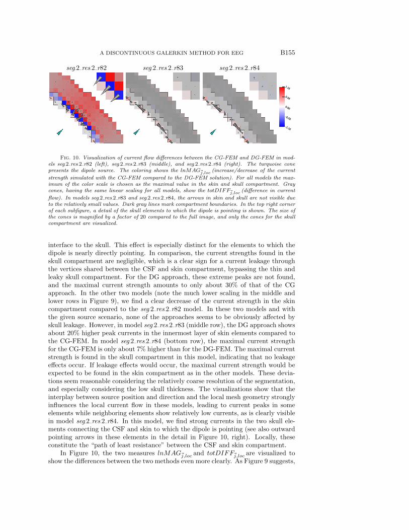
Fig. 10. Visualization of current flow differences between the CG-FEM and DG-FEM in mod-els seg 2 res 2 r82 (left), seg 2 res 2 r83 (middle), and seg 2 res 2 r84 (right). The turquoise conepresents the dipole source. The coloring shows the lnMAG~j,loc (increase/decrease of the current

strength simulated with the CG-FEM compared to the DG-FEM solution). For all models the max-imum of the color scale is chosen as the maximal value in the skin and skull compartment. Graycones, having the same linear scaling for all models, show the totDIFF~j,loc (difference in current

flow). In models seg 2 res 2 r83 and seg 2 res 2 r84, the arrows in skin and skull are not visible dueto the relatively small values. Dark gray lines mark compartment boundaries. In the top right cornerof each subfigure, a detail of the skull elements to which the dipole is pointing is shown. The size ofthe cones is magnified by a factor of 20 compared to the full image, and only the cones for the skullcompartment are visualized.

interface to the skull. This effect is especially distinct for the elements to which thedipole is nearly directly pointing. In comparison, the current strengths found in theskull compartment are negligible, which is a clear sign for a current leakage throughthe vertices shared between the CSF and skin compartment, bypassing the thin andleaky skull compartment. For the DG approach, these extreme peaks are not found,and the maximal current strength amounts to only about 30% of that of the CGapproach. In the other two models (note the much lower scaling in the middle andlower rows in Figure 9), we find a clear decrease of the current strength in the skincompartment compared to the seg 2 res 2 r82 model. In these two models and withthe given source scenario, none of the approaches seems to be obviously affected byskull leakage. However, in model seg 2 res 2 r83 (middle row), the DG approach showsabout 20% higher peak currents in the innermost layer of skin elements compared tothe CG-FEM. In model seg 2 res 2 r84 (bottom row), the maximal current strengthfor the CG-FEM is only about 7% higher than for the DG-FEM. The maximal currentstrength is found in the skull compartment in this model, indicating that no leakageeffects occur. If leakage effects would occur, the maximal current strength would beexpected to be found in the skin compartment as in the other models. These devia-tions seem reasonable considering the relatively coarse resolution of the segmentation,and especially considering the low skull thickness. The visualizations show that theinterplay between source position and direction and the local mesh geometry stronglyinfluences the local current flow in these models, leading to current peaks in someelements while neighboring elements show relatively low currents, as is clearly visiblein model seg 2 res 2 r84. In this model, we find strong currents in the two skull ele-ments connecting the CSF and skin to which the dipole is pointing (see also outwardpointing arrows in these elements in the detail in Figure 10, right). Locally, theseconstitute the “path of least resistance” between the CSF and skin compartment.

In Figure 10, the two measures lnMAG~j,loc and totDIFF~j,loc are visualized toshow the differences between the two methods even more clearly. As Figure 9 suggests,


we find for model seg 2 res 2 r82 that for the CG-FEM, the current strength is clearlyhigher than for the DG-FEM in those elements of the innermost layer of the skincompartment that share a vertex with the CSF compartment, indicated by the highlnMAG~j,loc (red coloring). The visualization of the totDIFF~j,loc (gray arrows) clearlyshows that the leakage generates a strong current from the CSF compartment directlyinto the skin compartment that does not exist for the DG-FEM. At the same time,the lnMAG~j,loc indicates that the current strength in the skull compartment is de-

creased in the CG-FEM (blue coloring); the detail of the skull elements for modelseg 2 res 2 r82 in Figure 9, left, actually shows that there is a stronger current throughthe skull elements in the DG-FEM than in the CG-FEM simulation (inwards pointingarrows). We also find high values for the totDIFF~j,loc in the CSF compartment thatare most probably caused by effects similar to the “leakage” effects, i.e., a mixingof conductivities in boundary elements/vertices. However, in model seg 2 res 2 r82,the color coding for the lnMAG~j,loc shows that this is not related to significant rela-tive differences in current strength. Here, the strongest values for the lnMAG~j,loc arefound in the skin and skull compartment. In turn, for the other two models we find thelargest deviations in the CSF compartment, both with regard to the totDIFF~j,loc andlnMAG~j,loc . For model seg 2 res 2 r83, we furthermore find minor effects with regardto the lnMAG~j,loc , i.e., relative differences of current strength, in the innermostlayer of skin elements, which are also the elements with the highest absolute currentstrength among the skin and skull compartment (see also Figure 9). We also findslightly increased values for the lnMAG~j,loc in the outermost layer of the skin ele-ments. These might be artifacts due to the “staircase”-like geometry of the outer sur-face in the regular hexahedral model. However, the totDIFF~j,loc in the skin and skullis negligible compared to the CSF compartment, and also clearly lower than in modelseg 2 res 2 r82. The same holds true for model seg 2 res 2 r84, where the lnMAG~j,loc isslightly increased in the skull and skin compartment, mainly in elements with a smallabsolute current strength, as a comparison to Figure 9 shows. Still, relatively highdifferences in the lnMAG~j,loc and totDIFF~j,loc are visible in the CSF compartment.These results indicate that the models seg 2 res 2 r83 and seg 2 res 2 r84 are less af-fected by skull leakage; the differences are due rather to the different computationalapproaches and do not show obvious errors due to the underlying segmentation.

For the realistic head models, 6CI hex 1mm and 6CI hex 2mm, the RDM andlnMAG in reference to model 6CI tet hr were computed. The cumulative relativefrequencies of the RDM and lnMAG are shown in Figure 11. At each position onthe x-axis, the corresponding y-value indicates the fraction of sources that have anRDM/lnMAG lower than this value. Accordingly, the rise of the curve should be assteep as possible for both the RDM and lnMAG and furthermore as close as possibleto the x=0 line for the lnMAG.

Overall, the results for both the RDM and lnMAG show relatively high errors.This is a consequence of the rather bad approximation of the geometry that is achievedwhen using regular hexahedra compared to the accuracy that can be achieved usinga surface-based tetrahedral model. While the differences between DG-FEM and CG-FEM observed for model 6CI hex 1mm are rather subtle, the differences are clear formodel 6CI hex 2mm. These results mainly underline the observations in the spherestudies.

In model 6CI hex 1mm, for both approaches about 50% of the sources show RDMerrors below 0.1 and 95% of the errors lie below 0.35. The rise of the curve for theDG-FEM is slightly steeper than for the CG-FEM, indicating a higher numerical


0

0.2

0.4

0.6

0.8

1

0 0.1 0.2 0.3 0.4 0.5

cum

. re

l. F

requen

cy

RDM

DG-FEM, 6CI_hex_1mm

DG-FEM, 6CI_hex_2mm

CG-FEM, 6CI_hex_1mm

CG-FEM, 6CI_hex_2mm

0

0.2

0.4

0.6

0.8

1

-0.2 -0.1 0 0.1 0.2 0.3 0.4 0.5 0.6

cum

. re

l. F

requen

cy

lnMAG

DG-FEM, 6CI_hex_1mm

DG-FEM, 6CI_hex_2mm

CG-FEM, 6CI_hex_1mm

CG-FEM, 6CI_hex_2mm

Fig. 11. Cumulative relative errors of the RDM (left) and lnMAG (right) in realistic six-layerhexahedral head models with 1- and 2-mm mesh resolutions in reference to high-resolution tetrahedralmodel.

Table 4Computational effort (from left to right): number of unknowns (DOFs), solving of a single

equation system (tsolve), overall computation time of transfer matrix (ttansfer), setup time of asingle right-hand side (trhs), overall computation time of leadfield matrix (tlf, 4,724 sources) andthe total computation time (ttotal).

DOFs tsolve ttransfer trhs tlf ttotal

6CI hex 1mm, DG 30,968,232 1,468 s 115,994 s 71 s 336,118 s 452,112 s

6CI hex 2mm, DG 3,876,256 136 s 10,750 s 8.8 s 41,939 s 52,689 s

6CI hex 1mm, CG 3,965,968 185 s 14,634 s 68 s 321,705 s 336,339 s

6CI hex 2mm, CG 508,412 20 s 1,588 s 8.7 s 41,222 s 42,810 s

accuracy, but from an RDM of about 0.3 onwards both curves are nearly overlapping.The RDM errors for the DG-FEM and CG-FEM are clearly increased for the lowermesh resolution. In this model, the difference between the DG-FEM and CG-FEMis also more distinct, e.g., for the DG-FEM more than 60% of the sources have anRDM below 0.2, but this is only the case for about 56% of the sources when usingthe CG-FEM.

The results for the lnMAG are in accordance with those obtained for the RDM.Again, the DG-FEM performs only slightly better than the CG-FEM in model6CI hex 1mm, whereas the differences in model 6CI hex 2mm are more distinct.

Compared to the results in the sphere models, the differences even in model6CI hex 2mm seem to be rather small. However, it has to be taken into account thatthe leakages in this model are nearly all located in temporal regions, so that only afraction of the sources is affected.

The computation times for the DG-FEM and CG-FEM in models 6CI hex 1mmand 6CI hex 2mm are shown in Table 4. All computation times are single CPU wall-clock times without exploitation of parallelization or vectoring. The solving time for asingle equation system tsolve grows approximately linearly with the number of degreesof freedom. This result corresponds to the theoretically predicted optimal scaling [16].Accordingly, the setup times for the transfer matrices, ttransfer, are clearly higher forthe DG-FEM than for the CG-FEM.

In contrast to the solving times, the setup times for a single right-hand side,trhs, differ only slightly between the CG-FEM and DG-FEM, being below 10 s for


model 6CI hex 2mm and around 70 s for model 6CI hex 1mm. For the source modelused here and the given number of sources, the overall computation time is clearlydominated by the computation of the right-hand sides. This part of the computationtakes twice as long as the setup of the transfer matrix even for the DG-FEM andmodel 6CI hex 1mm.

5. Discussion. In this paper we presented the theoretical derivation of the sub-traction FE approach for EEG forward simulations in the framework of DG methods.The scheme is consistent and fulfills a discrete conservation property. Existence anduniqueness follow from the coercivity of the bilinear form.

Numerical experiments in sphere models showed the convergence of the DG solu-tion toward the analytical solution with increasing mesh resolution and better approx-imation of the spherical geometry with increasing segmentation resolution. We alsoshowed that the numerical accuracy of the DG-FEM is dominated by the geometryerror, whereas the actual mesh resolution in a model with a bad geometry approxima-tion due to coarse segmentation resolution had only a minor influence on the numericalresults (Figure 6). The inaccurate representation of the geometry, especially for coarsemesh resolutions, is visible by the staircase-like boundaries in Figure 4.

In the comparisons of DG-FEM and the commonly used CG-FEM, we did notfind remarkable differences for models with higher mesh resolutions (1 mm, 2 mm),as the results in Figure 7 are in the same range for both approaches in the modelsseg 1 res 1 and seg 2 res 2. In this set of experiments, three main error sources can beidentified: geometry errors, numerical inaccuracies, and leakage effects.

First, there is the error in the representation of the geometry as a consequence ofapproximating the spherical models by voxel segmentations of different resolutions,which is increasing with coarser segmentation resolutions; see also Figure 6. We thusstrongly recommend the use of segmentation resolutions and, thereby, necessarily MRIresolutions, as high as practically feasible, possibly even locally refined when zoomedMRI technology is available. In fact, a newly developed zoom technique for MRI hasbecome available for practical use, based on a combination of parallel transmission ofexcitation pulses and localized excitation [15]. A first usage of this zoom techniquecan be found in [5] [4, Chapter 5]. Moreover, in future work, based on [11], we plan tofurther develop a cut-cell approach that allows for an accurate representation of thegeometry while introducing only a negligible number of additional degrees of freedom.Thus, the achieved accuracy can be increased while the computational effort is hardlyaffected (see first results in[34]).

Second, we have the numerical inaccuracy due to the discretization of (2.1) incombination with the strong singularity introduced by the assumption of a pointdipole, which is the main cause for the numerical inaccuracies of the subtractionapproach for highest eccentricities, where the source positions are very close to thenext conductivity jump (cf. Figure 7). A rationale for this effect has been given in[60, 25]. In future work, we are therefore planning to adapt other source modelingapproaches such as the Venant [47, 43, 18, 59, 52], the partial integration [61, 54,59, 48, 52], or the Whitney approach [46, 35, 36] to the DG-FEM framework. Untilnow, these have been formulated and evaluated only for the CG-FEM. Compared tothe subtraction approach, these approaches have the further advantage of a stronglydecreased computational effort for the setup of the right-hand-side vector [59, 52].

The third source of error, the “leakage effects,” explains the large differences innumerical accuracy between the CG-FEM and DG-FEM that can be observed inmodel seg 4 res 4. Due to the coarse resolution of the segmentation in comparison to


the thickness of the skull compartment (4-mm segmentation resolution, 6-mm skullthickness), this model can already be considered as (at least partly) leaky.

This observation motivated the further evaluation of the two methods in spheremodels with a thin skull compartment, where the assumed advantages of the DG-FEM should have a bigger effect. Therefore, we constructed spherical models witha thinner skull layer, assuming a skull thickness of 2–4 mm. The model with theminimal skull thickness of 2 mm, seg 2 res 2 r82, has a skull layer as thin as the edgelength of the hexahedrons (see Figures 8, 9, 10). Even though a mesh resolution of1 mm is strongly recommended for practical application of the FEM in source analysis[39, 7, 6], mesh resolutions of 2 mm are still used even in clinical evaluations [14], andthere are areas such as the temporal bone where the skull thickness is actually only 2mm or even less [30, Table 2], so that this is not an artificial scenario. As expected,the DG-FEM achieved a clearly higher numerical accuracy in the two models with thethinnest skull layers, seg 2 res 2 r82 and seg 2 res 2 r83, whereas the results for modelseg 2 res 2 r84 are comparable for the DG-FEM and CG-FEM (see Figure 8). In thelatter model, the ratio of resolution (2 mm) and skull thickness (4 mm) guarantees asufficient resolution and by this already prohibits leakages.

To make the difference between the CG-FEM and DG-FEM in the presence ofskull leakage better accessible, we generated Figures 9 and 10. The skull leakageis clearly visible in both figures for model seg 2 res 2 r82 and the CG-FEM as de-scribed in the results section. There is also a slight difference visible in the CSF inall three models, which might be explained by the relatively thin CSF layer. At thisresolution (2-mm CSF thickness, 2-mm segmentation resolution), the elements of theCSF compartment are no longer completely connected via faces, but often only viashared vertices (as visible in Figure 9, left column), which means that for such acoarse model, the current is blocked in some regions although in the real geometryit is not. In this case, the CG-FEM shows slightly better results, as it allows thecurrent to also flow through a single vertex, which is physically counterintuitive. Incontrast, the DG-FEM does exactly what one would intuitively expect from a meshbased on this segmentation: It channels the main current through the CSF, but dueto the wrong representation of the CSF in the segmentation it yields slightly wrongcurrents. It thereby reduces the usually very strong current in the highly conductiveCSF compartment, which might explain the slight advantages of the CG-FEM withregard to numerical accuracy for model seg 2 res 2 r84 (see especially the lnMAG inFigure 8), which is in agreement with the strong lnMAG effect of modeling the CSFas shown in [51, Figure 4]. Still, one has to point out that the wrong representationof the CSF geometry has only a very minor effect, as the current is not completelyblocked but only slightly diverted.

The findings for the sphere models were underlined by the results obtained usingrealistic six-compartment head models with mesh resolutions of 1 and 2 mm (Fig-ure 11). Also in this realistic scenario, the DG-FEM showed higher numerical accura-cies than the CG-FEM, especially for the lower mesh resolution of 2 mm. The leakagesin model 6CI hex 2mm are nearly exclusively found in temporal areas, whereas thesource positions are regularly distributed over the whole brain. Thus, only a fractionof the sources are strongly affected by leakage effects, and the observed differencesbetween the DG-FEM and CG-FEM in the realistic head model are not as large asone might assume from the results in model seg 2 res 2 r82, where the leakages areregularly distributed over the whole model.

Overall, these results show the benefits of the newly derived DG-FEM approachand motivate the introduction of this new numerical approach for solving the EEG


forward problem. Furthermore, the DG-FEM approach allows for an intuitive inter-pretation of the results in the presence of segmentation artifacts, which helps in theinterpretation of simulation results, in particular for clinical experts.

As we have shown in this study, errors in the approximation of the geometry as aresult of insufficient image or segmentation resolution and resulting current leakagesmight become significant when using hexahedral meshes. However, there are waysto avoid such errors. In [48], a trilinear immersed FEM to solve the EEG forwardproblem was introduced, which allows the use of structured hexahedral meshes, i.e.,the mesh structure is independent of the physical boundaries. The interfaces are thenrepresented by level sets and finally considered using special basis functions. However,this method is still based on the CG-FEM formulation, so that the behavior when thethickness of single compartments lies in the range of the resolution of the underlyingmesh is unclear, especially when both the compartment boundaries between the CSFand skull (inner skull surface) and skull and skin (outer skull surface) are containedin one element; it is probable that it suffers from the same problems as the commonCG-FEM in such cases. Unfortunately, no further in-depth analysis of this approachwas performed until now. Therefore, we claim to have for the first time presentedand evaluated an FEM approach preventing current leakage through single nodes.In future investigations, we intend to further develop the already discussed cut-cellDG approach for source analysis [34], which has the same advantageous features withregard to the representation of the geometry as the approach presented in [48], but,additionally, the charge preserving property of the DG-FEM as presented here.

The charge preserving property could also be achieved by certain implementa-tions of finite volume methods. In [20], a vertex-centered finite volume approach waspresented that shares the advantage that anisotropic conductivities can be treatedquite naturally with the here presented DG-FEM approaches. However, due to itsconstruction, the vertex-centered approach can also be affected by unphysical cur-rent flow between high-conducting compartments that touch in single nodes as seenfor the CG-FEM. This problem could be avoided using a cell-centered finite volumeapproach.

The evaluation of the computational costs of the DG-FEM and CG-FEM showeda higher computational effort for the DG-FEM for the solving of a single equationsystem and, in consequence, for the setup of the transfer matrices (Table 4). Thesolving times scaled linearly with the number of degrees of freedom, which correspondsto the theoretically predicted scaling [16]. The computation times for the setup of theright-hand side did not differ significantly between the CG-FEM and DG-FEM.

The computation of both the transfer matrix and the right-hand sides can beeasily parallelized by simultaneously solving multiple equation systems and setting upmultiple right-hand sides, respectively. This simple parallelization approach achievesan optimal scaling with the number of processors, cores, and SIMD lanes. Already aparallel computation of the transfer matrix on four cores, which can be considered asstandard equipment nowadays, would reduce ttransfer to about 8 h for the DG-FEMand model 6CI hex 1mm. This reduction of the computation time makes a practicalapplication feasible, since a computation could be carried out overnight. The use ofmore powerful equipment, as is available in many facilities, would allow for a furtherspeedup. However, in our experiments the overall computation times were dominatedby the setup of the right-hand side, which took twice as long as the transfer matrixsetup even for the more costly DG-FEM and model 6CI hex 1mm. This is a drawbackinherent to the subtraction approach. Its nice theoretical properties, which make itpreferrable for a first application with new discretization methodology, come at the


cost of a dense and expensive-to-compute right-hand side. For the CG-FEM, it wasshown that the setup time for the right-hand side vector can be drastically reducedby the adaptation of the direct source modeling approaches, such as Venant, partialintegration, or Whitney, that lead to a sparse instead of a dense right-hand-side vector,as previously discussed. For these approaches, the setup time for a single right-hand-side vector is reduced by up to two magnitudes [50]; a similar speedup can be expectedfor the DG-FEM. Furthermore, just as for the transfer matrix computation, for thecomputation of the right-hand sides an optimal speedup by parallelization can beeasily achieved.

Finally, since the DG approach allows fulfilling the conservation property of elec-tric charge also in the discrete case, it is not only attractive for source analysis, but alsofor the simulation and optimization of brain stimulation methods such as transcranialdirect or alternating current stimulation [24, 40, 57, 34, 53] or deep brain stimulation[19, 42].

6. Conclusion. We presented theory and numerical evaluation of the subtrac-tion FEM approach for EEG forward simulations in the DG-FEM framework. Weevaluated the accuracy and convergence of the newly presented approach in sphericaland realistic six-compartment models for different mesh resolutions and compared itto the frequently used Lagrange or CG-FEM. In common sphere models, we foundsimilar accuracies of the two approaches for the higher mesh resolutions, whereas theDG-FEM outperformed the CG-FEM for lower mesh resolutions. We further com-pared the approaches in the special scenario of a very thin skull layer where leakagesmight occur. We found that the DG approach clearly outperforms the CG-FEM inthese scenarios. We underlined these results using visualizations of the electric currentflow. The results for the sphere models were confirmed by those obtained in the re-alistic six-compartment scenario. The computation times presented in this study caneasily be reduced through parallelization. Furthermore, different approaches for thesetup of the right-hand side are expected to enable a major speedup without loss ofaccuracy to make a practical application of DG methods in EEG source analysis fea-sible. The DG-FEM approach might therefore complement the CG-FEM to improvesource analysis approaches.

REFERENCES

[1] Z. A. Acar and S. Makeig, Neuroelectromagnetic forward head modeling toolbox, J. Neurosci.Methods, 190 (2010), pp. 258–270.

[2] P. Antonietti and P. Houston, A class of domain decomposition preconditioners for hp-discontinuous Galerkin finite element methods, J. Sci. Comput., 46 (2011), pp. 124–149,https://doi.org/10.1007/s10915-010-9390-1.

[3] D. N. Arnold, F. Brezzi, B. Cockburn, and L. D. Marini, Unified analysis of discontinuousGalerkin methods for elliptic problems, SIAM J. Numer. Anal., 39 (2002), pp. 1749–1779.

[4] U. Aydin, Combined EEG and MEG Source Analysis of Epileptiform Activity Using Cali-brated Realistic Finite Element Head Models, PhD thesis, Fakultat fur Informatik undAutomatisierung, Technische Universitat Ilmenau, Germany, 2015, https://www.sci.utah.edu/∼wolters/PaperWolters/2015/Umit Aydin Dissertation 2015.pdf.

[5] U. Aydin, S. Rampp, A. Wollbrink, H. Kugel, J.-H. Cho, T. Knsche, G. C., W. J., andW. C. H., Zoomed MRI Guided by Combined EEG/MEG Source Analysis: A MultimodalApproach for Optimizing Presurgical Epilepsy Work-Up, manuscript.

[6] U. Aydin, J. Vorwerk, M. Dumpelmann, P. Kupper, H. Kugel, M. Heers, J. Wellmer,C. Kellinghaus, J. Haueisen, S. Rampp, H. Stefan, and C. Wolters, CombinedEEG/MEG can outperform single modality EEG or MEG source reconstruction in presur-gical epilepsy diagnosis, PLoS ONE, 10 (2015), e0118753, https://doi.org/10.1371/journal.pone.0118753.

https://doi.org/10.1007/s10915-010-9390-1

https://www.sci.utah.edu/~wolters/PaperWolters/2015/Umit_Aydin_Dissertation_2015.pdf

https://www.sci.utah.edu/~wolters/PaperWolters/2015/Umit_Aydin_Dissertation_2015.pdf

https://doi.org/10.1371/journal.pone.0118753

https://doi.org/10.1371/journal.pone.0118753


[7] U. Aydin, J. Vorwerk, P. Kupper, M. Heers, H. Kugel, A. Galka, L. Hamid, J. Wellmer,C. Kellinghaus, S. Rampp, S. Hermann, and C. Wolters, Combining EEG and MEGfor the reconstruction of epileptic activity using a calibrated realistic volume conductormodel, PloS ONE, 9 (2014), e93154.

[8] P. Bastian, M. Blatt, A. Dedner, C. Engwer, R. Klofkorn, R. Kornhuber,M. Ohlberger, and O. Sander, A generic grid interface for parallel and adaptive sci-entific computing. Part II: Implementation and tests in DUNE, Computing, 82 (2008),pp. 121–138, https://doi.org/10.1007/s00607-008-0004-9.

[9] P. Bastian, M. Blatt, A. Dedner, C. Engwer, R. Klofkorn, M. Ohlberger, andO. Sander, A generic grid interface for parallel and adaptive scientific computing. PartI: Abstract framework, Computing, 82 (2008), pp. 103–119, https://doi.org/10.1007/s00607-008-0003-x.

[10] P. Bastian, M. Blatt, and R. Scheichl, Algebraic multigrid for discontinuous Galerkindiscretizations of heterogeneous elliptic problems, Numer. Linear Algebra Appl., 19 (2012),pp. 367–388, https://doi.org/10.1002/nla.1816.

[11] P. Bastian and C. Engwer, An unfitted finite element method using discontinuous Galerkin,Internat. J. Numer. Methods Eng., 79 (2009), pp. 1557–1576.

[12] P. Bastian, F. Heimann, and S. Marnach, Generic implementation of finite element methodsin the distributed and unified numerics environment (DUNE), Kybernetika (Prague), 46(2010), pp. 294–315.

[13] O. Bertrand, M. Thevenet, and F. Perrin, 3D finite element method in brain electricalactivity studies, in Biomagnetic Localization and 3D Modelling, J. Nenonen, H. M. Rajala,and T. Katila, eds., Technical report, Department of Technical Physics, Helsinki Universityof Technology, Helsinki 1991, pp. 154–171.

[14] G. Birot, L. Spinelli, S. Vulliemoz, P. Megevand, D. Brunet, M. Seeck, and C. Michel,Head model and electrical source imaging: A study of 38 epileptic patients, NeuroImageClinical, 5 (2014), pp. 77–83.

[15] M. Blasche, P. Riffel, and M. Lichy, Timtx trueshape and syngo zoomit technical andpractical aspects, Magnetom Flash, 1 (2012), pp. 74–84.

[16] D. Braess, Finite Elements: Theory, Fast Solvers, and Applications in Solid Mechanics,Cambridge University Press, Cambridge, 2007.

[17] R. Brette and A. Destexhe, Handbook of Neural Activity Measurement, Cambridge Univer-sity Press, Cambridge, 2012, https://doi.org/10.1017/CBO9780511979958.

[18] H. Buchner, G. Knoll, M. Fuchs, A. Rienacker, R. Beckmann, M. Wagner, J. Silny, andJ. Pesch, Inverse localization of electric dipole current sources in finite element models ofthe human head, Electroencephalog. Clinical Neurophys., 102 (1997), pp. 267–278.

[19] C. Butson, S. Cooper, J. Henderson, and C. McIntyre, Patient-specific analysis of the vol-ume of tissue activated during deep brain stimulation, NeuroImage, 34 (2007), pp. 661–670.

[20] M. Cook and Z. Koles, A high-resolution anisotropic finite-volume head model for EEGsource analysis, in Proceedings of the 28th Annual International Conference of the IEEEEngineering in Medicine and Biology Society, IEEE, Piscataway, NJ, 2006, pp. 4536–4539.

[21] J. de Munck and M. Peters, A fast method to compute the potential in the multi spheremodel, IEEE Trans. Biomed. Eng., 40 (1993), pp. 1166–1174.

[22] D. Di Pietro and A. Ern, Mathematical Aspects of Discontinuous Galerkin Methods, Math.Appl. (Berlin), 69, Springer, Berlin, 2011.

[23] D. A. Di Pietro, A. Ern, and J.-L. Guermond, Discontinuous Galerkin methods foranisotropic semidefinite diffusion with advection, SIAM J. Numer. Anal., 46 (2008),pp. 805–831.

[24] J. Dmochowski, A. Datta, M. Bikson, Y. Su, and L. Parra, Optimized multi-electrodestimulation increases focality and intensity at target, J. Neural Eng., 8 (2011), 046011.

[25] F. Drechsler, C. Wolters, T. Dierkes, H. Si, and L. Grasedyck, A full subtraction ap-proach for finite element method based source analysis using constrained Delaunay tetra-hedralisation, NeuroImage, 46 (2009), pp. 1055–1065.

[26] N. Gencer and C. Acar, Sensitivity of EEG and MEG measurements to tissue conductivity,Phys. Med. Biol., 49 (2004), pp. 701–717.

[27] S. Giani and P. Houston, Anisotropic hp-adaptive discontinuous Galerkin finite elementmethods for compressible fluid flows, Int. J. Numer. Anal. Model., 9 (2012), pp. 928–949.

[28] A. Gramfort, T. Papadopoulo, E. Olivi, and M. Clerc, Forward field computation withOpenMEEG, Comput. Intell. Neurosc., 2011 (2011), 923703 https://doi.org/10.1155/2011/923703.

https://doi.org/10.1007/s00607-008-0004-9

https://doi.org/10.1007/s00607-008-0003-x

https://doi.org/10.1007/s00607-008-0003-x

https://doi.org/10.1002/nla.1816

https://doi.org/10.1017/CBO9780511979958

https://doi.org/10.1155/2011/923703

https://doi.org/10.1155/2011/923703


[29] M. Hamalainen, R. Hari, R. J. Ilmoniemi, J. Knuutila, and I. Lounasmaa,Magnetoencephalography—theory, instrumentation, and applications to noninvasive stud-ies of the working human brain, Rev. Modern Phys., 65 (1993), pp. 413–497.

[30] J.-H. Kwon, J. Kim, D.-W. Kang, K.-S. Bae, and S. Kwon, The thickness and textureof temporal bone in brain CT predict acoustic window failure of transcranial doppler, J.Neuroimaging, 16 (2006), pp. 347–352.

[31] G. Marin, C. Guerin, S. Baillet, L. Garnero, and G. Meunier, Influence of skullanisotropy for the forward and inverse problem in EEG: Simulation studies using theFEM on realistic head models, Human Brain Mapping, 6 (1998), pp. 250–269.

[32] V. Montes-Restrepo, P. van Mierlo, G. Strobbe, S. Staelens, S. Vandenberghe, andH. Hallez, Influence of skull modeling approaches on EEG source localization, BrainTopography, 27 (2014), pp. 95–111.

[33] J. Mosher, R. Leahy, and P. Lewis, EEG and MEG: Forward solutions for inverse methods,IEEE Trans. Biomed. Eng., 46 (1999), pp. 245–259.

[34] A. Nuessing, C. Wolters, H. Brinck, and C. Engwer, The unfitted discontinuous Galerkinmethod for solving the EEG forward problem, IEEE Trans. Biomed. Eng., 63 (2016),pp. 2564–2575.

[35] S. Pursiainen, A. Sorrentino, C. Campi, and M. Piana, Forward simulation and in-verse dipole localization with the lowest order Raviart-Thomas elements for electroen-cephalography, Inverse Problems, 27 (2011), 045003, https://doi.org/10.1088/0266-5611/27/4/045003.

[36] S. Pursiainen, J. Vorwerk, and C. Wolters, Electroencephalography (EEG) forward model-ing via H(div) finite element sources with focal interpolation, Phys. Med. Biol., 61 (2016),8502.

[37] C. Ramon, P. Schimpf, and J. Haueisen, Influence of head models on EEG simulationsand inverse source localizations, BioMed. Eng. OnLine, 5 (2006), https://doi.org/10.1186/1475-925X-5-10.

[38] B. Riviere, M. F. Wheeler, and V. Girault, A priori error estimates for finite elementmethods based on discontinuous approximation spaces for elliptic problems, SIAM J. Nu-mer. Anal., 39 (2002), pp. 902–931.

[39] M. Rullmann, A. Anwander, M. Dannhauer, S. Warfield, F. Duffy, and C. Wolters,EEG source analysis of epileptiform activity using a 1 mm anisotropic hexahedra finiteelement head model, NeuroImage, 44 (2009), pp. 399–410.

[40] R. Sadleir, T. Vannorsdall, D. Schretlen, and B. Gordon, Target optimization in tran-scranial direct current stimulation, Front. Psychiatry, 3 (2012), p. 90.

[41] P. Schimpf, C. Ramon, and J. Haueisen, Dipole models for the EEG and MEG, IEEE Trans.Biomed. Eng., 49 (2002), pp. 409–418.

[42] C. Schmidt, P. Grant, M. Lowery, and U. van Rienen, Influence of uncertainties in thematerial properties of brain tissue on the probabilistic volume of tissue activated, IEEETrans. Biomed. Eng., 60 (2013), pp. 1378–1387.

[43] R. Schonen, A. Rienacker, R. Beckmann, and G. Knoll, Dipolabbildung im FEM-Netz,Teil I, Arbeitspapier zum Projekt Anatomische Abbildung elektrischer Aktivitat des Zen-tralnervensystems, RWTH Aachen, University/Aachen 1994.

[44] H. Sonntag, J. Vorwerk, C. Wolters, L. Grasedyck, J. Haueisen, and B. Maess, Leakageeffect in hexagonal FEM meshes of the EEG forward problem, in International Conferenceon Basic and Clinical Multimodal Imaging (BaCI), 2013.

[45] M. Stenroos and J. Sarvas, Bioelectromagnetic forward problem: Isolated source approachrevis(it)ed, Phys. Med. Biol., 57 (2012), pp. 3517–3535.

[46] O. Tanzer, S. Jarvenpaa, J. Nenonen, and E. Somersalo, Representation of bioelectriccurrent sources using Whitney elements in finite element method, Phys. Med. Biol., 50(2005), pp. 3023–3039.

[47] R. Toupin, Saint-Venants principle, Arch. Ration. Mech. Anal., 18 (1965), pp. 83–96, https://dx.doi.org/10.1007/BF00282253.

[48] S. Vallaghe and T. Papadopoulo, A trilinear immersed finite element method for solving theelectroencephalography forward problem, SIAM J. Sci. Comput., 32 (2010), pp. 2379–2394.

[49] F. Vatta, F. Meneghini, F. Esposito, S. Mininel, and F. D. Salle, Solving the forwardproblem in EEG source analysis by spherical and FDM head modeling: A comparativeanalysis, Biomed Sci Instrum, 45 (2009), pp. 382–388.

[50] J. Vorwerk, New finite element methods to solve the EEG/MEG forward problem, PhDthesis, Mathematisch-Naturwissenschaftliche Fakultat, Westfalische-Wilhelms Univer-sitat Munster, Germany, 2016, https://www.sci.utah.edu/∼wolters/PaperWolters/2016/Vorwerk Dissertation 2016.pdf.

https://doi.org/10.1088/0266-5611/27/4/045003

https://doi.org/10.1088/0266-5611/27/4/045003

https://doi.org/10.1186/1475-925X-5-10

https://doi.org/10.1186/1475-925X-5-10

https://dx.doi.org/10.1007/BF00282253

https://dx.doi.org/10.1007/BF00282253

https://www.sci.utah.edu/~wolters/PaperWolters/2016/Vorwerk_Dissertation_2016.pdf

https://www.sci.utah.edu/~wolters/PaperWolters/2016/Vorwerk_Dissertation_2016.pdf


[51] J. Vorwerk, J.-H. Cho, S. Rampp, H. Hamer, T. Knosche, and C. Wolters, A guideline forhead volume conductor modeling in EEG and MEG, NeuroImage, 100 (2014), pp. 590–607,https://dx.doi.org/10.1016/j.neuroimage.2014.06.040.

[52] J. Vorwerk, M. Clerc, M. Burger, and C. Wolters, Comparison of boundary element andfinite element approaches to the EEG forward problem, Biomedizinische Technik. Biomed-ical engineering, 57 (2012).

[53] S. Wagner, S. Rampersad, U. Aydin, J. Vorwerk, T. Oostendorp, T. Neuling, C. Her-rmann, D. Stegeman, and C. Wolters, Investigation of tDCS volume conduction effectsin a highly realistic head model, Journal of Neural Engineering, 11 (2014), p. 016002(14pp).https://dx.doi.org/10.1088/1741-2560/11/1/016002.

[54] D. Weinstein, L. Zhukov, and C. Johnson, Lead-field bases for electroencephalography sourceimaging, Annals of Biomedical Engineering, 28 (2000), pp. 1059–1066.

[55] K. Wendel, N. Narra, M. Hannula, P. Kauppinen, and J. Malmivuo, The influence ofCSF on EEG sensitivity distributions of multilayered head models, IEEE Transactions onBiomedical Engineering, 55 (2008), pp. 1454–1456.

[56] M. Wheeler, An elliptic collocation-finite element method with interior penalties, SIAM Jour-nal on Numerical Analysis, 15 (1978), pp. 152–161.

[57] M. Windhoff, O. A., and T. A., Electric field calculations in brain stimulation based onfinite elements: an optimized processing pipeline for the generation and usage of accurateindividual head models, Human Brain Mapping, 34 (2013), pp. 923–35.

[58] C. Wolters, L. Grasedyck, and W. Hackbusch, Efficient computation of lead field bases andinfluence matrix for the FEM-based EEG and MEG inverse problem, Inverse Problems,20 (2004), pp. 1099–1116.

[59] C. Wolters, H. Kostler, C. Moller, J. Hardtlein, and A. Anwander, Numericalapproaches for dipole modeling in finite element method based source analysis, Inter-national Congress Series, 1300 (June 2007), pp. 189–192. ISBN-13:978-0-444-52885-8,https://dx.doi.org/10.1016/j.ics.2007.02.014.

[60] C. Wolters, H. Kostler, C. Moller, J. Hardtlein, L. Grasedyck, and W. Hackbusch,Numerical mathematics of the subtraction method for the modeling of a current dipole inEEG source reconstruction using finite element head models, SIAM Journal on ScientificComputing, 30 (2007), pp. 24–45.

[61] Y. Yan, P. Nunez, and R. Hart, Finite-element model of the human head: scalp potentials dueto dipole sources, Medical and Biological Engineering and Computing, 29 (1991), pp. 475–481.

https://dx.doi.org/10.1016/j.neuroimage.2014.06.040

https://dx.doi.org/10.1088/1741-2560/11/1/016002

https://dx.doi.org/10.1016/j.ics.2007.02.014

Documents

A DISCONTINUOUS GALERKIN METHOD TO SOLVE THE EEG …wolters/ChildBrainPapers/...A DISCONTINUOUS GALERKIN METHOD FOR EEG B139 to solve the underlying partial di erential equations in