Embed Size (px)
Citation preview

A Computable General Equilibrium (CGE) Approach to Urban Freshwater
Planning
Stages 2 and 3: Methodology and Data Requirements
Report prepared for the Chief Economist
Unit, Auckland Council
May 2017
The Chief Economist Unit (CEU) at Auckland Council commissioned this study on behalf of the Ministry for Environment (MfE) and provided general oversight of the project. The focus is on the feasibility of incorporating freshwater-quality planning into a sub-regional Computable General Equilibrium (CGE) model.
This report has been authored by John Kim and peer reviewed by Dr. Adolf Stroombergen.
Contact person: Harshal Chitale harshal.chitale@auck;landcouncil.govt.nz
1
The study has been divided into four stages:
1. Literature review of Computable General Equilibrium (CGE) models in analysing the impacts on freshwater quality
2. Advice about how to develop the sub-regional housing CGE model to incorporate impacts on freshwater quality
3. Inputs and data requirements to run the CGE model identified in (2), and inputs available
4. Final report and presentation.
This report focuses on the second and the third stages of the study, where we aim to:
a) Outline the most appropriate methodology for studying the freshwater-quality issues as identified in the first stage of the study
b) Provide a description of the current sub-regional housing CGE model and how freshwater quality can be incorporated
c) Outline the data requirement including the description of a New Zealand multi-regional social accounting matrix.
2
Table of Contents Executive Summary ............................................................................................................................................................. 4
Background ........................................................................................................................................................................ 4
What is a CGE Model? ..................................................................................................................................................... 4
Why use CGE models to assess policies about the quality of fresh water? ............................................ 4
Why incorporate freshwater-quality planning into the CEU sub-regional housing CGE model? ....................................................................................................................................................... 8
What are the three key concerns about using the CGE model? ................................................................... 6
How might the CGE model benefit the council’s planning initiatives? .................................................... 7
1 Introduction to this report and purpose of main study ............................................................................ 8
1.1 Water as an important natural resource .............................................................................................. 8
1.2 A new model to analyse planning initiatives, including for water ............................................ 9
1.3 Key advantages of the CGE model over other EIA models ........................................................... 9
1.4 Objectives of this report ........................................................................................................................... 11
Stage 2: Advise how the sub-regional housing CGE model can be developed
to incorporate impacts on freshwater quality ............................................................................................ 11
Stage 3: Inputs required to run a CGE model, and inputs available (gap analysis) ....................................................................................................................................................................... 11
1.5 Summary of Stage 1: The literature review ..................................................................................... 11
1.6 Outline of the rest of this report .......................................................................................................... 13
2 Framework of the Computable General Equilibrium model ................................................................ 14
2.1 Key considerations on developing the sub-regional CGE model ............................................ 14
2.1.1 Method 1: a generic, multi-regional CGE framework ............................................................. 15
2.1.2 Method 2: two regions within a multi-regional model .......................................................... 16
2.1.3 Method 1 as the preferred method ................................................................................................. 16
2.2 Sub-regional housing component......................................................................................................... 16
2.3 The module for managing the quality of fresh water .................................................................. 17
2.4 Specification of the sub-regional CGE model with freshwater quality
management ................................................................................................................................................................... 19
2.4.1 How the baseline CGE models prices............................................................................................. 20
2.4.2 Transforming the output..................................................................................................................... 20
2.4.3 Modelling pollution ............................................................................................................................... 24
2.4.4 Demand for commodities ................................................................................................................... 25
2.4.5 The relationship between household income and tax ........................................................... 30
2.4.6 Trade with the rest of the world ...................................................................................................... 30
2.4.7 Market clearing and model closure ................................................................................................ 31
2.4.8 Numerical specification of the model ............................................................................................ 31
2.5 Incorporating the policy instruments for managing the quality of fresh
water 32
3
2.5.1 Freshwater limits ................................................................................................................................... 32
2.5.2 Prioritising how fresh water is allocated ..................................................................................... 33
2.5.3 Incorporating social value into the model .................................................................................. 33
2.6 Development programme for building an integrated model ................................................... 33
2.6.1 The four groups within the project team ..................................................................................... 35
2.6.2 The project’s Five key deliverables ................................................................................................ 36
2.6.3 Risks to completing the project successfully ............................................................................. 36
3 Stage 3: Gap analysis on data requirements and the value of the study ......................................... 38
3.1 Overview of the data requirements ..................................................................................................... 38
3.1.1 Social accounting matrix ..................................................................................................................... 38
3.1.2 Spatial economic data ........................................................................................................................... 39
3.2 New Zealand National Social Accounting Matrices ...................................................................... 39
3.3 Building the social accounting matrices for the sub-regional model ................................... 40
3.3.1 The 2013 National Social Accounting Matrix ............................................................................. 40
Data requirements for the National Social Accounting Matrix ............................................................ 46
3.3.2 The multi-regional Social Accounting Matrix ............................................................................ 47
Constructing the regional supply-use table ................................................................................................. 47
Balancing the RSUT ................................................................................................................................................. 56
Constructing the RSAM ......................................................................................................................................... 56
3.3.3 The sub-regional Social Accounting Matrix ................................................................................ 66
3.4 Data requirements for incorporating a freshwater module .............................................................. 66
4 Summary and Conclusions .................................................................................................................................. 68
4.1 Summary of Stage 2 .................................................................................................................................... 68
4.2 Summary of Stage 3 .................................................................................................................................... 68
4.3 Conclusions..................................................................................................................................................... 68
4.3.1 A summary of how the CGE model assesses freshwater quality ....................................... 69
4.3.2 The benefits of using an expanded CGE model to assess the
implications of both freshwater quality and other economic initiatives........................................ 70
References ............................................................................................................................................................................ 72
Appendix A Freshwater Instruments for Economic Modelling ............................................................. 77
Appendix B Data Sources for NSAM ................................................................................................................... 80

4
Executive Summary
Background
The Chief Economist Unit (CEU) at the Auckland Council commissioned this
study on behalf of the Ministry for Environment to assess the feasibility of incorporating freshwater-quality planning into the sub-regional housing
Computable General Equilibrium (CGE) model that the CEU is developing.
This study includes: (i) a review of national and international practices of using a
CGE model to assess economic impacts of freshwater-quality policy initiatives;
(ii) a description of the current sub-regional housing CGE model and how to
incorporate a freshwater-quality component; and (iii) an outline of model inputs and data requirements.
What is a CGE Model?
CGE is a methodology that models the economy and the various inter-
relationships between economic sectors. It models decision makers such as
consumers, producers and the Government in terms of how they make their
choices. Decision makers are assumed to be rational in the sense that their consumption and production decisions aim to maximise their welfare by
responding to changes in costs and prices.
CGE models are useful for capturing the effects of a new policy (e.g. freshwater
quality standards, tariffs, carbon taxes) or an external shock that affects
economic activity (e.g. natural disasters, global market events). The model is able to calculate the impact of this change on the choices and welfare levels of
consumers and producers and the consequent effects on the economy as a whole.
The impacts on economic activity calculated in a CGE model include direct,
indirect and induced impacts.
In addition to how much of a commodity is produced and consumed, the model includes financial flows within the economy (e.g. transfer payments, government
revenue and expenditure). The model can then be simulated for different values
of parameters set outside the model itself. Such parameters may include
different income distributions or policy variables, such as tax and subsidy
profiles and water quality standards.
CGE models are used widely within New Zealand and internationally. Many
government agencies build and maintain CGE models for economic projections
and Economic Impact Assessments (EIA) of policies. These include a high-level
New Zealand CGE model built by the Treasury for economic forecasting as well
as assessing impacts of trade policies, and a multi-regional transport CGE model built by the New Zealand Transport Agency (NZTA) to assess economic
consequences of road outages. Further, CGE models have been used to assess
economic impacts associated with greenhouse gas policies.
Why use CGE models to assess policies about the quality of fresh water?
Internationally, CGE models are widely used to assess the economic implications
of freshwater policy initiatives, particularly on economic growth. However,

5
within New Zealand, most EIAs of water policies are use a mix of Cost–Benefit
Analysis (CBA) and Input-output (IO) analysis.
CBA and IO do not inherently include an entire economy. In contrast, the CGE
model provides a more comprehensive EIA as it simulates a complete economy. Importantly, the supply and demand forces within the CGE model ensure that
the economic impacts associated with a policy initiative are not over-estimated,
unlike a partial-equilibrium or an IO approach.1 So the CGE model provides
robust economic impact outputs associated with a policy on the quality of fresh
water.
The CGE model can show how what we make and consume helps to generate
water pollutants within an economy. In addition, the model can include changes
in how economic participants behave. One example is when a producer adjusts
the way they produce and invest when abatement technology behaviours change
following a change in policy. The model also includes detailed financial flows. Specifically, the model can track changes in central and local government
finances as a result of a policy.
The model can be used to assess the economic impacts of urban development,
planning and growth policies on freshwater quality, and how policy about the
quality of fresh water affects the economy. Similarly, the model can include other environmental policies (e.g., greenhouse gas emission) and show feedback
effects on freshwater quality, as well as interaction effects between freshwater
and environmental policies.
Increases in population2 and urbanisation3 change the structure of an economy.
Especially for a growing city such as Auckland, these increases can substantially affect freshwater use and quality. Unlike CBA and IO, which cannot assess
structural changes in the economy, the CGE model can assess the direction and
the magnitude of the structural change and associated freshwater use and
quality.
Systems Dynamic Models are sometimes used to study the economic impacts of events such as natural disasters or major policy changes. A particular version of
that is used to analyse the impacts of infrastructure outages is essentially a two-
region model and not a multi-regional one. It is not a general equilibrium model
but tries to mimic one. Whether it does a good job of doing so is an open
question. The model can be hard to run and requires the use of experts which can be costly. It is also not as flexible as general equilibrium models and cannot
be easily adapted to different contexts or lines of enquiry. A flexible CGE model
can likely be developed in the cost it would take to learn to use or get experts to
run a systems dynamic model on a repeated basis.
1 This is illustrated in the paper by Deng et al. (2011)[12]. Using a CGE model, the authors applied
a production tax to industries that intensively produce nitrogen and phosphorous emissions. Resulting changes in emission outputs and economic outputs were not a one-to-one relationship; emissions decreased by 1.62 percent while economic output decreased by only 1.08 percent.
2 Watson and Davies (2011)[60] found that a 50 percent increase in population in Colorado
resulted in a 5.7 percent shift in water use from agriculture industry to non-agriculture industry. 3 Jiang et al. (2014)[20] note that urbanisation in China raises the opportunity cost of water use,
and so shifts water use from lower-value and water-intensive agriculture to higher-value livestock farming. Water use and economic output from farming field farming dropped by 11.2 percent and 19.4 percent respectively, while livestock farming increased by 24.6 percent and 17.5 percent respectively.

6
Why incorporate freshwater-quality planning into the CEU sub-regional housing CGE model?
A policy initiative in a geographical area can affect not only the area but
surrounding areas as well. In addition, policies can affect each area differently
and interdependencies between areas cause feedback effects. From a regional
policymaking perspective, it is important to understand possible winners and
losers of a policy as aggregate metrics will underestimate the magnitude of economic impacts that different groups within a region feel.
The CEU sub-regional CGE model includes inter-spatial relationships within the
Auckland region and the rest of New Zealand. Therefore, the model can assess
how a policy in a region or a sub-region can affect surrounding regions and
identify winners and losers and the sub-regional distribution of the economic impacts of the policy. This can improve our understanding of the spatial
distribution of the economic costs and benefits of policies.
The Auckland region consists of multiple Freshwater Management Unit (FMU)
areas where each FMU differs in economic activities, land use, and geophysical
characteristics. Different characteristics across FMUs lead to distinct economic responses given the same policy on the quality of fresh water. Importantly, a
single regional model does not allow for FMU-specific policies and the FMU-
specific characteristics are averaged into a regional characteristic.
Incorporating freshwater-quality planning into the CEU sub-regional CGE model
at FMU level allows us to model FMU specific characteristics, policies and economic responses. The model has the advantage of capturing inter-FMU
feedbacks and reflecting the real world more closely. So it has the potential to
provide more robust and disaggregated results and to show the distribution of
economic impacts across space for FMU-specific policies on the quality of fresh
water. The model also facilitates an analysis of FMU based on the impacts of policy measures at the regional and national levels.
What are the key concerns about using the CGE model?
The CGE model has major advantages over other EIA methods, yet the model is
quite difficult to build and operate. Three key concerns are noted below.
First, the proposed multi-regional CGE model requires a large amount of detailed
data. Specifically, robust sub-regional economic and water accounts data is required to build an FMU-level model. Often this is lacking, but data can be
calculated numerically and updated when superior data becomes available.
Second, building the CGE model is a highly technical process. New Zealand has
only a handful of CGE experts, but some people within our private organisations
and academic institutions have CGE experience.
Third, although CGE models are proven to be robust and tested over many years,
the model employs strong assumptions. For policies on the quality of fresh water,
assumptions such as perfect competition within a market and symmetry of
information may not necessarily reflect reality. Yet these assumptions are
inherent in most economic models and are handled within the CGE model by designing scenarios around these assumptions.

7
How might the CGE model benefit the council’s planning initiatives?
There is increasing pressure on land in Auckland due to rapidly growing
population. Also, land that is used for housing, industry or agriculture pollutes
our freshwater resources and policies that limit freshwater pollution will impose
difficult choices on us as we grow. Freshwater policies may impose constraints
or make us think hard about the quantity and type of economic activities that can be carried out on our land. A model that can answer questions about how
different freshwater management units are affected and how their management
via policy in turn affects economic activity across Auckland will be a valuable
tool to possess.
The FMU-level, sub-regional CGE model for Auckland Council will potentially enable the council to robustly assess the consequences of policy initiatives
focused on freshwater quality. In addition, building the model will develop the
capability to assess the economic impact of future policies not only for Auckland
but for other New Zealand regions.
8
1 Introduction to this report and purpose of the
study
Over the past decade, Auckland has experienced tremendous economic and
population growth. Its key consequence has been intensified urbanisation within
Auckland. As a result, Auckland Council (the Council) faces policy setting issues
that involve balancing growth objectives against consequent environmental
externalities that are difficult to quantify. Two key issues the council is facing are housing affordability (Parker, 2015[40]; Torshizian and Chitale, 2016[58]) and
how to fund future infrastructure growth and manage urban growth spatially
and over time.
The purpose of this study is to understand the potential to expand the scope of
the sub-regional Computable General Equilibrium (CGE) model that Auckland Council was proposing to develop, so that it can also account for impacts of
freshwater policies under the National Policy Statement for Freshwater
Management (NPS-FM) on urban growth and economic development and vice
versa.
In particular, this study looks at a particular configuration of a model whose specification incorporates a freshwater-quality management module into a
broader CGE modelling framework. We identify some of the key challenges to
this exercise and some specific data requirements.
1.1 Water as an important natural resource
Water is an important natural resource essential for our society and for the
biophysical environment we live in. As with most other public goods, positive
externalities of clean water are not fully captured. In addition, as a result of the free-rider problem (when the benefits of a resource are enjoyed without paying
for it), people and entities in an economy have little incentive to care for the
quality of water. This means, the public sector must intervene to secure clean
water supply for society.
The NPS-FM requires regional councils to set objectives for their community consensus about the future role of their water catchments and to set limits.4 To
meet the objectives, the council is required to implement a detailed plan, setting
rules and regulations on how to manage fresh water in each region. Yet the
economic implications of setting the plan are still unclear and difficult to
measure. In particular, expansion of the urban footprint in Auckland may incur considerable mitigation costs in adhering to the NPS-FM. The imposed costs will
be a significant burden to the public and the council, potentially causing regional
growth that is less than ideal. This stresses the need for tools to analyse the costs
of growth and find less costly means of achieving growth.
4 See the ‘About the National Policy Statement for Freshwater Management’ web page, Ministry for
the Environment. Retrieved on 27 February from www.mfe.govt.nz/fresh-water/national-policy-
statement/about-nps
9
1.2 A new model to analyse economic impacts of planning initiatives
The Chief Economist Unit (CEU) of Auckland Council is considering the
development a sub-regional housing CGE model to analyse the economic
consequences of current policy and planning initiatives within Auckland (with a
focus on affordability issues).
One key characteristic of the model being considered for development is that it is a multi-regional model for use also at a sub-regional level. The Auckland region
is spatially separated into smaller sub-regions. Specifically, the region is split
into sub-regions using Statistics New Zealand (SNZ) 2013 Community Board5
(CB) boundaries. This allows for a feedback between sub-regions (i.e., CBs), and
shows the sub-regional distribution of the economic impacts of policies and planning. Importantly, the model was intended to be able to assess the inter-
regional distribution of the economic impacts, winners and losers associated
with exogenous shocks and policy settings.
The proposed model could be applied in various scenarios. It has the potential to
evaluate the effects of policy interventions on economic outcomes in various sectors within the Auckland region. In addition, the model structure and
implementation (e.g., computer codes) could be applied to other spatial
definitions (e.g., other regions in New Zealand).
1.3 Key advantages of the CGE model over other EIA models
In the literature review conducted in Stage 1 of the study, we found numerous
studies supporting the use of CGE models in assessing the economic implications of environmental policy initiatives. We have identified benefits of a sub-regional
CGE model and the key advantages that the model has over other Economic
Impact Assessment (EIA) methods (i.e., CBA) and Input-output (IO)). Eight key
advantages are noted below.
1. Unlike partial equilibrium models (i.e., CBA and IO), CGE models both the supply and demand side for every economic activity. This allows the model
to assess the economic consequences of urban development, land-use
planning and growth policies on freshwater quality, and on how policy
decisions about the quality of fresh water affect the economy and land use.
2. CGE models incorporates price dynamics, where an exogenous shock to the economy affects prices of commodities (which, in turn, affects how
people and entities in an economy produce and consume commodities).
3. While the CBA and the IO methods inherently do not include an entire
economy, the CGE model simulates a complete economy. As noted above,
the model includes physical flows (i.e., production and consumption) and financial flows (i.e., subsidies and transfers) within the economy. This
means the model provides a complete picture of the economic
consequences associated with a policy.
5 Community Boards within Auckland are also known collectively as the Auckland Local Board
Area. That Area has 21 sub-regions.
10
4. The model can be used to test the economic impacts of various policies in a
standardised setting. This occurs once the underlying structure and
formulation 6 of the CGE model is standardised, and the base CGE model is
set up. In such tests, it is possible to compare different policies and calculate the opportunity costs (i.e., compare the economic impacts of
policy A against policy B).
5. Extending the above point, the CGE model allows for the modelling of the
economic consequences of other national and local government policies
(e.g., on taxation and on greenhouse gas emission) in conjunction with freshwater policy measures. For example, a CGE model could assess the
economic impacts associated with a greenhouse gas policy, and how it
affects freshwater quality, to give us a better understanding of the
interaction effect between regulating carbon emission and limiting water
contaminants.
6. The proposed CEU sub-regional housing CGE model incorporating the
management module on freshwater quality is designed to model how both
production and consumption activities within an economy help to
generate water pollution. In addition, the proposed model incorporates an
endogenous abatement module where producers within the economy adjust what they produce and how they behave in response to policy
changes. The model can simulate the behaviour of agents within an
economy and estimate economic impacts associated with introducing
policies with set limits. In particular, the model can be used to test and
compare various policies on water quality.
7. Most importantly, the model is multi-regional, where Auckland is spatially
separated by the Freshwater Management Units7 (FMUs) and includes
other areas of New Zealand. Each FMU has different economic activities,
land use, and geophysical characteristics. Further, different characteristics
across FMUs lead to distinct economic responses for the same policy for different FMUs. As such, a simple regional model does not allow for FMU
specific policies as the FMU specific characteristics are averaged into
regional characteristics.
8. The proposed model includes, for each FMU, specific freshwater-quality
issues, water supply, and land use characteristics, and economic activities. The proposed model can run specific policy scenarios for each FMU area. It
has the advantage of capturing inter-FMU/inter-regional feedbacks and
reflects the real world more closely. It therefore provides more robust
results (compared to a regional CGE model) and shows the distribution of
economic impacts across space for numerous FMU specific policies about the quality of fresh water. The model also facilitates an analysis of FMU
based on the impacts of policy measures at the regional and national levels.
6 The CEU sub-regional housing CGE model is built in a Mathematical Programming Subsystem
for General Equilibrium (MPSGE) programming language. The mathematical complexities of a CGE model increase rapidly with increase in variables, such as more areas and industries. A large CGE model, such as the CEU sub-regional housing model becomes computationally hard to solve. This problem is encountered in the CGE model constructed in a standard Mixed Complementary Problem (MCP) language or other methods, when the model and outputs become unstable. By comparison, the MPSGE is highly robust in dealing with large CGE models. 7 See sections 2.3 and 3.3.3 for more detail.
11
1.4 Objectives of this report
This report examines two main stages of the study: stages 2 and 3. The two
stages involve a detailed feasibility study on incorporating the freshwater
planning into a sub-regional Computable General Equilibrium (CGE) model.
Outlined below is an excerpt from the original proposal by the Chief Economist Unit (CEU) to the Ministry for the Environment (MfE).
Stage 2: Advise how the sub-regional CGE model can be developed to incorporate impacts of freshwater quality
• Describe the potential to incorporate externalities from water quality deterioration into the CEU’s proposed CGE framework and how this would be implemented. Comment on the associated risks and issues.
• Advise on a rough development programme, and outline the resource
requirements (skills, time, budget etc.) in case the project is progressed to the next stage.
Stage 3: Inputs required to run a CGE model, and inputs available (gap
analysis)
• Find existing data on freshwater quality for CGE analysis.
• Recommend a research programme to implement CGE model that
accounts for impacts on freshwater quality, and outline the data requirement and the value for money of doing so.
• Coarse estimates of further parameters needed for successful application
of the CGE model.
1.5 Summary of Stage 1: The literature review
In Stage 1 of the study, we conducted a literature review of the existing literature
and methodologies with regard to the economic impact of freshwater-quality management using CGE modelling. The literature surveyed for this project
mainly concerned whether applying CGE modelling might help us understand the
economic impact of environmental policies.
Our review found that work on models specifically focusing on water-quality
policies is lacking. Even so, the papers surveyed contained some useful freshwater-economic modules focused on pollution abatement.
A majority of papers surveyed incorporated a separate pollution abatement
sector whose ‘output’ is pollution clean-up. Xie and Saltzman (2000)[61] models
pollution taxes, subsidies, and clean-up activities in an integrated economic and
environmental CGE model. The services provided by the pollution abatement sector are assumed to be a ‘public good’ that production sectors can buy so as to
comply with environmental regulations, and the government can buy.
Dellink, Hofkes, Ierland and Verbruggen (2004) [10] offer more details about
abatement technologies and the costs of abating pollution. Among the multiple
12
pollutants specified in paper by Dellink et al., water quality is measured primarily
by nutrient loadings of nitrogen and phosphorus. The Cass-Koopmans-Ramsey
type model takes pollution as a necessary environmental input into the
production process. The supply of abatement goods is modelled through a separate producer, and the government sets environmental policy by limiting the
number of tradeable pollution permits it issues.
Bohringer and Loschel (2006) [4] also endogenise pollution control by creation
of clean-up sectors and modelling pollutant directly into production. Further, it
specifies a wage curve depicting the inverse relationship between the level of wages and the rate of unemployment. Brouwer, Hofkes and Linderhof (2008) [6]
include substitution elasticities between labour, capital, and emissions to water
in the sector production function. A static CGE model is built and the results are
downscaled to river-basin level. The producers buy emission rights and invest in
abatement technologies. The model explicitly distinguishes between abatable and unabatable pollution.
Deng, Zhao, Wu, Lu and Dai (2011)[12] have built another multi-regional
environmental CGE model. They specifically look into the nitrogen and
phosphorus emissions in China and its impact on economic growth. An
alternative approach outlined in the literature survey is to model multiple types and uses of water. Luckmann, Grethe, McDonal, Orlov and Siddig (2013) [28]
allow for substitution and price differentiation in the production and use of
different water qualities. Water production is represented as a separate,
independent activity with a specific cost structure. Different cost structures are
implemented by the imposition of policy instruments such as taxes and subsidies. Also, some limitations of CGE modelling on sustainability are outlined. Scrieciu
(2006) [43] comments that the CGE models are too primitive to capture most
environmental concerns.
In New Zealand, most EIAs of water policies were conducted using a combination
of CBA and IO approach and, at time of writing this report, no completed studies focused on water policies using a CGE approach. Several studies used a partial-
equilibrium approach focusing on farm systems. Even so, we did find two CGE
studies currently under way by Environment Southland, and research project
funded by the Ministry of Business, Innovation and Employment (MBIE) and led
by GNS Science—a Crown Research Institute (CRI).
In particular, one key objective of the former study is to build CGE modelling
capacity within the council so that, in future, it can do its own EIAs using the CGE
model.
In summary, we have found numerous cases supporting the use of CGE models to
assess economic implications of water quality and other environmental policy initiatives in Auckland.8 A review of the international literature revealed that CGE
models are widely used to help assess the economic implications of
environmental policies, particularly those related to economic growth and water
quality. The studies on water quality we reviewed were conducted fairly recently,
and we noted a growing interest in the issue of water quality.
8 Importantly, some studies raised concerns about strong assumptions, such as perfect
competition and symmetric information, required within the CGE model. However, these assumptions are inherent in most economic models, and can be offset by designing scenarios and the study around these assumptions.

13
1.6 Outline of the rest of this report
The rest of this report is organised in three stages.
Stage 2 proposes the most suitable model to incorporate freshwater-quality issues into the sub-regional housing CGE model
Stage 3 discusses the data requirements, with a focus on how the Social
Accounting Matrices (SAM) are built
Stage 4 provides the report’s summary and conclusions.
14
2 Framework of the Computable General
Equilibrium model
CGE modelling has the distinct advantage of capturing inter-related markets and
secondary (indirect and induced) impacts in evaluating the net economic effects
of policies to the economy. To understand the economic impacts associated with
setting limits for the quality of fresh water, the proposed CEU sub-regional CGE
can be modified to incorporate freshwater quality as an endogenous factor within the model.
This section starts off with subsection 2.1, which outlines important
considerations when developing the sub-regional CGE model. Subsection 2.2
describes the housing module within the CGE model. Subsection 2.3 outlines the
management module for freshwater quality within a CGE model framework. Subsection 2.4 provides functional specifications of the sub-regional housing
CGE model. Subsection 2.5 then describes how the policy instrument for
managing freshwater quality is incorporated into the CGE model outlined in
subsection 2.4. Finally, subsection 2.6 outlines a possible development
programme of the CEU sub-regional housing CGE model for managing freshwater quality.
2.1 Key considerations in developing the sub-regional CGE model
Auckland consists of a large urban area, has more than 1.6 million people and
contributes to more than a third of New Zealand’s GDP. The region has
considerable spatial variations in economic and demographic profiles as well as
geographical characteristics. These variations cause sub-regions to respond
differently to exogenous factors, such as policy changes, economic growth and population changes. In conducting an Economic Impact Assessment (EIA), it is
important to analyse not only aggregated regional impacts but how each sub-
region is affected and the magnitude of variations within it. For regional
policymaking, it is important to understand possible winners or losers of
exogenous policy shocks within a region, as aggregate metrics are likely to underestimate the magnitude of economic impacts felt by different members
(spatially separated in this example) within a region.
To address this issue, the CEU’s proposed CGE framework is a sub-regional CGE
model—a multi-regional CGE model with the Auckland region spatially
separated into CB-level sub-regions. This allows for feedback between sub-regions and shows sub-regional distribution of the economic impacts.
Subsequently, the proposed CGE model for freshwater quality is a sub-regional,
multi-regional CGE model. As noted earlier, geophysical and economic
characteristics across Auckland vary significantly. As such, channels of water
pollution within Auckland will differ spatially.
The proposed model will consist of sub-regions separated by FMUs within
Auckland, and consist of regions in the rest of New Zealand. This allows the CGE
model to incorporate spatial variations in pollution channels between different
FMUs and report FMU-level economic impacts and responses by agents within
the economy from the initiatives for setting freshwater-quality limits. Further,
the model allows for heterogeneous policies to be applied across the FMUs,
15
where these policies can be set based on differing pollution characteristics of
each FMU. This allows for more detailed evaluation of policies and for
optimisation of costs and benefits of achieving the target.
Theoretically, a generic multi-regional CGE model framework9 consists of spatially explicit economies but contains the same agents (e.g., government,
household and enterprise), class of industries (e.g., horticulture, dairy farming
and manufacturing) and commodities (e.g., raw milk, automobile and insurance).
Each region in the model follows similar, if not identical, mathematical
formulations. The differences in regional economic responses are driven by varying regional factor (e.g., labour and capital) costs and commodity prices,
where regional factor costs are determined by supply of regional employment
and available capital. The commodity prices are mostly determined by regional
differences in production methods and transportation costs.
Building a realistic and rationally sound sub-regional multi-regional CGE model is more complicated as forces that drive the regional differences in a generic
multi-regional model (e.g., transport costs between regions) do not apply
strongly within a region. For example, in a generic multi-regional CGE model, the
main constraint restricting the size of an economy may be the total labour force
available in the region.
In the short run, and given the size of the labour force is fixed, the only way to
increase a region’s labour force is through people coming from other regions to
live and be employed there. In reality, the labour force and people in general do
not immigrate easily between regions other than for economic reasons. In
economics, this phenomenon is termed “sticky labour force mobility” and is modelled within the multi-regional CGE model through a mathematical function
describing the trade-off between the negative utilities from moving between
regions against the positive utilities (such as higher wages) from moving.
Yet, in a sub-regional CGE model, people do not need to move between the sub-
regions to ensure economic growth in the sub-region and to participate in other sub-regions economic activities. For example, a person living in West Auckland
does not have to move to central Auckland for a job. In addition, commodity and
factor prices, and parameters driving the CGE model framework, are unlikely to
vary enough to cause differences between sub-regions. As such, it will be
unrealistic to model a sub-regional, multi-regional CGE model using a generic multi-regional CGE model framework.
Alternatively, two possible methods are available to model the sub-regional
characteristics.
2.1.1 Method 1: a generic, multi-regional CGE framework
In the first method, the sub-regional CGE model will be formulated using a
generic multi-regional CGE framework but can incorporate a regional market for
factors of production (e.g., labour and capital). It will use Armington elasticities
that are specific to each sub-region to measure commodities within a main region.
9 The most widely known CGE model using this framework is the Global Trade Analysis Project
(GTAP). GTAP is a multi-national global CGE model looking into economics of international trade.

16
The regional market for factors combines all sub-regional factors and distribute
across sub-regions. In effect, factors in a region have identical prices across the
sub-regions and can include elasticities that can govern the mobility factor
between sub-regions. For example, Auckland can have a single labour market where all sub-regional labour forces gather and are subsequently distributed
across the region at the same labour price. But labourers in North Auckland are
less likely to work in South Auckland.
Also, by including sub-regional commodity elasticities, sub-regional demand of
commodities produced within a region can be tuned to match sub-regional dynamics. For example, a person in North Auckland may value, and so price, a
car in south Auckland the same as a person pricing the same type of car on the
north shore. Yet the same person may value their hair dressing services in south
Auckland differently to the person doing hair dressing on the north shore. The
advantage of using this method is that it can include detailed sub-regional production and demand dynamics, such as different sub-regional household
types (e.g., income distribution). Even so, including additional market and
certain Armington elasticities adds complexities and increases data
requirements to the model.
2.1.2 Method 2: two regions within a multi-regional model
In the second method, the industries of a region in the CGE model consist of sub-
regional industries. In this method, the CGE model only has Auckland and the
rest of New Zealand as two regions within a multi-regional CGE model. But industries within Auckland region are subdivided into sub-regional industries.
For example, the Auckland dairy industry will be subdivided into North
Auckland dairy industry and South Auckland dairy industry.
If required, the method can also include sub-regional agent types within a region
(e.g., north Auckland households and south Auckland households). This method is simpler than the first method, as it does not require additional markets. Also, it
models trade interactions between sub-regions but does not model differences
in sub-regional demands. For example, a person visiting a hair dresser in north
Auckland may value, and so price, a hair dresser in north Auckland the same
they would value, and so price, a hair dresser in south Auckland.
2.1.3 Method 1 as the preferred method
The sub-regional model component of the CEU CGE model is currently being
developed and is not at the stage where specifications and methods are decided. Both methods outlined above have distinctive merits. Although the preferred
method is the Method 1, computational complexities and extra data
requirements may mean that method cannot be applied. Therefore, further
research and trial application of both methods is required before building a full
sub-regional model.
2.2 Sub-regional housing component
Within the current sub-regional CGE model, housing is a commodity consumed by households and is an output from a productive sector. Production function for
the housing commodity shares the same functional form as other commodities,
but includes the residential land supply as an additional factor of production.
Supply of the total available residential land is an exogenous function of the

17
model and set by the council zoning and density rule parameters. A simple policy
assessment is possible by changing these parameter values. The actual supply of
residential land is an endogenous linear function of the price of residential land
and the total available residential land.
Housing demands follow the household utility maximisation function, with a
minimum level of housing commodity consumption modelled using a Linear
Expenditure System (LES) function. As the labour and population are inter-
related in the model, the factor movement between the study areas influences
the level of housing commodity demanded within a study area. Currently, the non-economic values of housing (e.g., environment, amenities and location) are
not included, as the model assumes that the values are constant parameters and
the base is a steady state comprising all of these.
By including freshwater quality into the CGE model, non-economic values
related to the freshwater quality can change within the model. For example, an increase in freshwater quality in a sub-region increases the environmental value.
This, in turn, increases demand for housing within the sub-region. This process
can be modelled using two endogenous functions; (i) an endogenous labour
mobility, where the population is a function of non-economic housing values and
wage; and (ii) an endogenous housing LES ratio, where the minimum level of housing demand is a linear function of non-economic housing values and
population within the sub-region.
It is important to note that, the specification of the sub-regional housing module
requires further work. Proposed future extensions to the module include
disaggregating the household into multiple types and splitting the housing commodity into different types of housing (e.g., stand-alone and apartments).
2.3 The module for managing the quality of fresh water
The proposed CEU sub-regional CGE model is designed to be built as a multi-
regional CGE model (in this case, CBs of Auckland and other parts of
New Zealand) to allow for separate region/area-specific supply issues, prices,
local government policies, and production functions, as well as imperfect factor
mobility between regions. Before going into the details of the freshwater-quality management modules, it is important to note that the CGE model incorporating
freshwater quality will be spatially separated by the FMUs. This means that the
spatial areas of the sub-regional housing CGE model must be re-specified from
CBs to FMUs.
This re-specification involves matching the CB boundaries against FMU boundaries and disaggregating/aggregating CBs to match FMU areas. It is
important to note that the FMU boundaries follow geophysical characteristics
while the CB boundaries follow economic and demographic characteristics. This
can potentially cause some FMU areas having no economic rationale to be a sub-
region within the CGE model. As such, the total number of sub-regions within the model will depend upon the economic viability of FMU sub-regions, where any
FMUs not viable are merged into a surrounding FMU.
Technically, the multi-regional CGE model, which the sub-regional CGE model is
classed as, will add origin and destination subscripts to variables and equations.
This means that production sectors (i.e., firms), final demand sectors (e.g., government and households), and factors (e.g., labour and capital) may all be

18
specific to each separate region. We will need data that describes the economic
links (e.g., inter-regional trade) between the regions for the multi-regional SAM.
For example, for each type of commodity in the model, the two-region system
will demand a set of two-by-two trade matrices consisting of information about inter-regional imports and exports.
In a CGE framework, the environmental policies could be effectively modelled by
incorporating these policies as endogenous factors. Within the framework,
pollution is modelled as a by-product of consumption and production. On the
production side, a producer’s total cost could include pollution related costs from pollutant emission restrictions. This will come in the form of pollution
emission taxes, limits, and the cost of removing pollution to comply with
environmental quality standards. In effect, the industrial polluters are required
to pay compensation to the society for the environmental damage they cause. On
the consumption side, the households are required to pay for pollution they incur, such as the tax to treat sewage. This reduces the amount of money they
have available for other consumables.
In the limit-setting initiatives for freshwater quality, the water quality will be
measured primarily by nutrient loadings of nitrogen and phosphorus, Total
Suspended Solids (TSS), and heavy metals (i.e., copper, lead and zinc).10 Within the CGE freshwater-quality module, the water pollution will be modelled
explicitly as a necessary environmental input for the production and utility
functions. Therefore, it will include substitution elasticities between labour,
capital, intermediate consumption (goods and services used in production
activities), and emissions to water from industrial production.
The government could use various policy instruments to set the standard for
freshwater quality. Such options may include setting a cap on emission, a
pollution tax, and auctioning a restricted number of tradeable pollution permits.
The producer has to produce up to a permissible emission level, pay pollution
tax, buy emission rights or adhere to the limit-setting policy. In addition, a producer can make investment decisions in abatement technologies or change
their production technology to meet the emission limit.
The module can assume no change in production input requirements under the
freshwater-quality limit as a benchmark scenario. Or it can feature an abatement
technology module to build in detailed changes in the production input requirement as a response to policy shocks. The choice a producer faces, of
whether to pay for the pollution or increase their investment on pollution
abatement technologies, is endogenised. The abatement cost curve will slope
down and represent abatement costs as a function of pollution.
A Constant Elasticity of Substitution (CES) function is estimated to best fit the abatement cost curve. The estimated CES elasticity describes the possibility of
substituting between pollution and investing in abatement technologies. It
reflects marginal abatement costs, which is how much additional abatement
effort is needed to reduce pollution by one extra unit.
The abatement technology can be modelled as a commodity produced by a separate production sector using both intermediate goods and factors of
10 The measures of water quality depend on the list of public instruments of the local government,
and on the available datasets.
19
production as inputs. All economic agents can invest in the available abatement
technologies by buying the abatement technology commodity. So the trade-off is
between investing in abatement technologies and reducing economic activity.
Simply put, if you reduce economic activity you reduce emissions.
The model will calculate the abatement functions by calibrating the data derived
from the abatement cost curves. The function consists of abatable (can be
reduced by increasing the input of abatement goods) and unabatable
(proportional to output) pollution.
To model the government costs associated with cleaning up water pollution, the model can incorporate a separate water-pollution clean-up module, whose
output is the pollution clean-up. The module can be used to test various funding
mechanisms for clean-up activities. For example, the module can assume the
services to clean up freshwater pollution are a ‘public good’ that the production
sectors buy to comply with environmental regulations, the government buys, or both buy. Households usually have no has demand for services to clean up water
pollution.
Lastly, to model degradation of water qualities and its effects on production
activities, multiple types of water with different qualities can be directly
incorporated into the CGE model. Specifically, the water pollution can reduce the availability of high-quality water as a factor of production and change the input
technology for production. This means industries are forced to use sub-optimal
production technology, resulting in a lower output of industrial commodities.
In this model, water production is represented as a distribution activity that
supplies water to the activities of producing and consuming other commodities. Those activities in turn create water pollution that in turn feeds back into the
water production process. This module enables a wide range of simulations
focused on freshwater-related policy. For example, local government can assess
the cost and benefits of investing in water treatment plants across the whole
economy.
Although out of scope for this study, one way to improve the freshwater-quality
module would be to allow the environmental parameters to change over time,
incorporating the effects of diffusion of abatement technology, innovation,
learning effects and exogenous technological progress in pollution efficiency.
The current parameters govern the changes in technical potential for pollution reduction and efficiency improvements in the abatement sector. Subsequently,
exogenous parameters drive the development in the abatement possibilities and
costs while the diffusion of existing abatement technology is endogenised.
2.4 Specification of the sub-regional CGE model with freshwater quality management
The model specified in this section is a CGE model following a standard Arrow-
Debreu general equilibrium framework.11 1213 For an illustrative purpose, the
11 The Arrow-Debreu general equilibrium framework is based on a seminal paper by Kenneth
Arrow and Gerard Debreu. The framework forms a basis for most general equilibrium models where, under a set of assumptions (e.g., convexity of consumption and production decisions, and perfect competition) market clearing prices exist (i.e., in an economic system where the amount demand equals the amount supplied).

20
model described in the next section is simplified as a static, single-region and
has a single pollution measure. The full model specification will be a dynamic,14
multi-regional CGE model containing multiple sources of pollution. The
pollution is modelled as an endogenous commodity used for production and consumption activities, and abatement is modelled as an investment to reduce
the cost of pollution. Policy instruments can be set exogenously or endogenously
within the model. For example, a limit-setting policy that affects the marginal
costs of production can enter into the model as an endogenous variable related
to the production output level. Further details on incorporating the proposed policy instruments on freshwater management into the CGE model are given in
section 2.5 of this report.
In addition, pollution limits can be represented by an emission cap and a
pollution tax, where the tax rates are set exogenously. Both can be used at the
same time to simulate the policy instruments. Government sets the emission cap and industries adjust their optimal production and abatement technology
investment behaviours endogenously.
The pollution tax is explicitly outlined within the model to simulate the optimal
trade-off behaviour of those industries that face both emissions costs imposed
by the government (in this case, a pollution tax) and voluntary clean-up costs. Specifications of the pollution tax are outlined in section 2.4.3 of this report.
2.4.1 How the baseline CGE models prices
The baseline CGE model represents 10 different groups of average prices. These include:
composite good price
domestic good prices
capital input prices
the domestic prices of imports and exports
the prices of intermediate inputs
value-added prices
the world prices of imports
exports and output prices.
The capital input prices are set either exogenously or endogenously depending
on the model closure. For example, the wage rate can be assumed fully flexible to
let the supply of labour equal demand or, alternatively, unemployment can be
modelled to represent the labour market supply and demand imbalance.
2.4.2 Transforming the output
We assume that each production sector uses intermediate goods along with
other factors of production. The industries are assumed to be perfectly competitive. They engage in joint production so that each industry can produce
12 Currently, the model is programmed in a General Algebraic Modelling System (GAMS)
programming language. 13 The model specification is as outlined in Kim (2013) [23]. 14 Most dynamic CGE models are built using either a recursive (i.e., sequential) approach or an
inter-temporal (i.e., across time) approach. The CGE model outlined in this report can be adopted for both approaches. The suitable dynamics within the dynamic CGE model will vary depending on the design of the freshwater-quality scenario.

21
more than one type of commodity. A commodity from different industries is
assumed to be differentiated and therefore not perfectly substitutable. This
means that the elasticity of transformation regarding joint production is set
relatively inelastic.
The outputs are either consumed domestically or exported, and they follow the
Constant Elasticity of Transformation (CET) Armington specification. 15 We
assume Constant Returns to Scale (CRS), and the factors of production include
labour, capital, land, and water pollution and water quality. These are combined
by the CES production function. Intermediate goods are a mix of domestic and imported goods, and are incorporated into production by the Leontief
production function. They are assumed to be heterogeneous and follow the CES
function. Figure 1 illustrates the production flow.
15 The CET and Armington specification is explained in further detail in section 2.4.6.

22
Figure 1: Production flowchart of the economy
Figure 1 describes the inputs and outputs of production activities within the CGE model. Inputs, consisting of domestic and imported commodities and factors of production (labour, capital and land), are used to produce outputs that are either exported or consumed domestically.
Each industry solves the profit maximisation problem with zero economic profit.
The equation that demonstrates the industry’s optimisation problem for a firm (j) is:
subject to ,
23
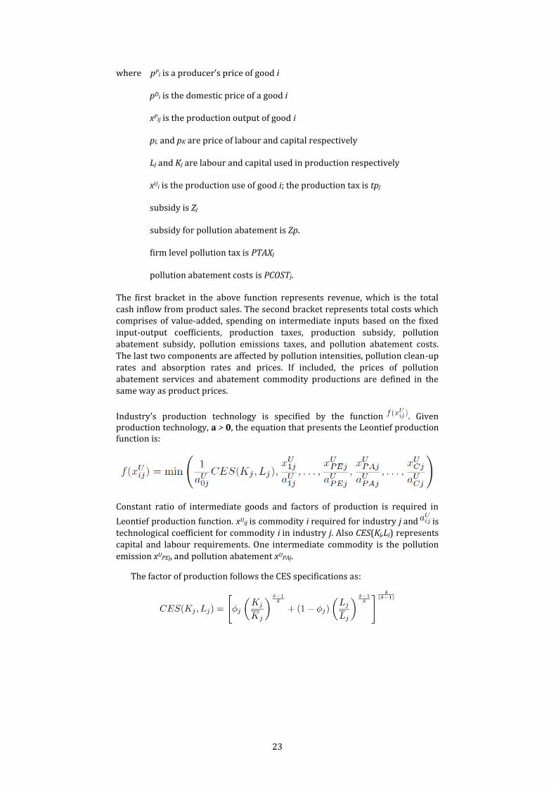
where pPi is a producer’s price of good i
pDi is the domestic price of a good i
xPij is the production output of good i
pL and pK are price of labour and capital respectively
Lj and Kj are labour and capital used in production respectively
xUi is the production use of good i; the production tax is tpj
subsidy is Zj
subsidy for pollution abatement is Zp.
firm level pollution tax is PTAXj
pollution abatement costs is PCOSTj.
The first bracket in the above function represents revenue, which is the total
cash inflow from product sales. The second bracket represents total costs which comprises of value-added, spending on intermediate inputs based on the fixed
input-output coefficients, production taxes, production subsidy, pollution
abatement subsidy, pollution emissions taxes, and pollution abatement costs.
The last two components are affected by pollution intensities, pollution clean-up
rates and absorption rates and prices. If included, the prices of pollution
abatement services and abatement commodity productions are defined in the same way as product prices.
Industry’s production technology is specified by the function . Given production technology, a > 0, the equation that presents the Leontief production function is:
Constant ratio of intermediate goods and factors of production is required in
Leontief production function. xUij is commodity i required for industry j and is technological coefficient for commodity i in industry j. Also CES(Kj,Lj) represents
capital and labour requirements. One intermediate commodity is the pollution
emission xUPEj, and pollution abatement xUPAj.
The factor of production follows the CES specifications as:
24
where is capital16 to labour ratio in industry j; δ is the elasticity of substitution; Kj and Lj are capital and labour used in production respectively; and
Kj and Lj are baseline capital and labour used in production respectively.
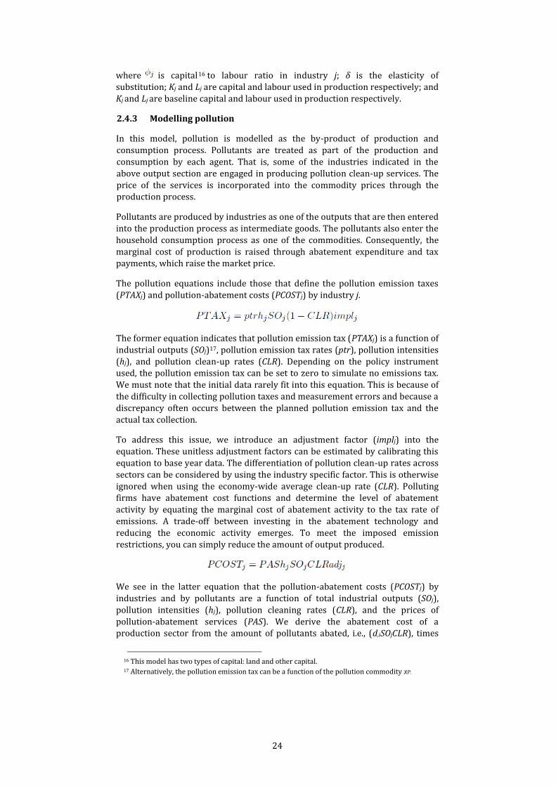
2.4.3 Modelling pollution
In this model, pollution is modelled as the by-product of production and
consumption process. Pollutants are treated as part of the production and
consumption by each agent. That is, some of the industries indicated in the
above output section are engaged in producing pollution clean-up services. The
price of the services is incorporated into the commodity prices through the production process.
Pollutants are produced by industries as one of the outputs that are then entered
into the production process as intermediate goods. The pollutants also enter the
household consumption process as one of the commodities. Consequently, the
marginal cost of production is raised through abatement expenditure and tax payments, which raise the market price.
The pollution equations include those that define the pollution emission taxes
(PTAXj) and pollution-abatement costs (PCOSTj) by industry j.
The former equation indicates that pollution emission tax (PTAXj) is a function of
industrial outputs (SOj)17, pollution emission tax rates (ptr), pollution intensities
(hj), and pollution clean-up rates (CLR). Depending on the policy instrument used, the pollution emission tax can be set to zero to simulate no emissions tax.
We must note that the initial data rarely fit into this equation. This is because of
the difficulty in collecting pollution taxes and measurement errors and because a
discrepancy often occurs between the planned pollution emission tax and the
actual tax collection.
To address this issue, we introduce an adjustment factor (implj) into the
equation. These unitless adjustment factors can be estimated by calibrating this
equation to base year data. The differentiation of pollution clean-up rates across
sectors can be considered by using the industry specific factor. This is otherwise
ignored when using the economy-wide average clean-up rate (CLR). Polluting firms have abatement cost functions and determine the level of abatement
activity by equating the marginal cost of abatement activity to the tax rate of
emissions. A trade-off between investing in the abatement technology and
reducing the economic activity emerges. To meet the imposed emission
restrictions, you can simply reduce the amount of output produced.
We see in the latter equation that the pollution-abatement costs (PCOSTj) by
industries and by pollutants are a function of total industrial outputs (SOj),
pollution intensities (hj), pollution cleaning rates (CLR), and the prices of
pollution-abatement services (PAS). We derive the abatement cost of a production sector from the amount of pollutants abated, i.e., (d,iSOjCLR), times
16 This model has two types of capital: land and other capital. 17 Alternatively, the pollution emission tax can be a function of the pollution commodity xP.

25
the price of pollution clean-up (PAS). The dollar is the unit used for both sides of
the equation.
2.4.4 Demand for commodities
Demand for commodities comprises household consumption demand,
government consumption demand, export demand, intermediate inputs,
investment demand, and inventory. The household consumption activity emits
pollution, represented here by consumption of the pollution commodity.
(i) Households: Households are the main supplier of labour to productive
industries and the main consumer of produced commodities. They receive
wage and transfers from other agents and spend their income on
commodity consumption, savings and payments to other agents.
Household commodities demand depends on maximising the utility of their CES utility function subject to income constraint. Households
consume both domestic and imported goods and each domestic
commodity i is assumed to be not identical to the imported commodity i
using the CES function.
Figure 2 illustrates the household demand and supply flow.
A household’s disposable income function is specified as:
The above equation describes the disposable income of a household where
the left bracket is income and the right bracket is expenditure except commodity consumption. The household receives CoEH, compensation for
labour (GOSH), their share of the capital return and transfer payments
from enterprise (eh), government (gh), and rest of the world (ROW)
(rowh). Total income is taxed at th rate. Household expenditures are
transfer payments to enterprise (he), government (hg), ROW (hrow), savings (hs), and household pollution tax (PTAXH). Household savings are
assumed to be exogenous and do not affect consumption decisions.18
The problem of maximising utility for households is set out in Figure 2
below.
18 We could incorporate a waste disposal services as a lump-sum transfer from each household to
the local government.
26
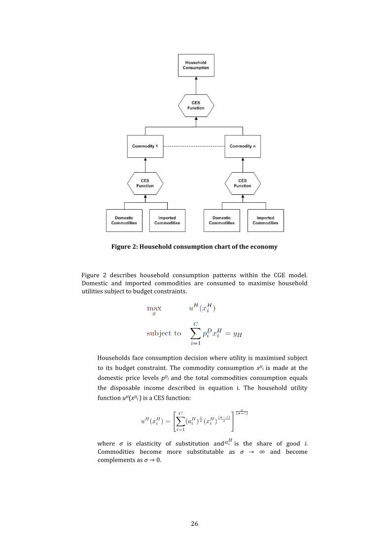
Figure 2: Household consumption chart of the economy
Figure 2 describes household consumption patterns within the CGE model. Domestic and imported commodities are consumed to maximise household utilities subject to budget constraints.
Households face consumption decision where utility is maximised subject
to its budget constraint. The commodity consumption xHi is made at the
domestic price levels pDi and the total commodities consumption equals
the disposable income described in equation i. The household utility
function uH(xHi ) is a CES function:
where σ is elasticity of substitution and is the share of good i.
Commodities become more substitutable as σ → ∞ and become
complements as σ → 0.

27
The household demand function for commodities is:
Household demand for commodity xk, where k ≠ i, depends on the domestic
price of the commodity j, the average price of all other goods, and the
elasticity of substitution σ.
(ii) Government: Government takes two forms: central government and local
government. The main source of income for both forms of government is
tax revenue from other agents. The government also consumes
commodities, provides transfers to households and subsidises industries.19
The government’s consumption pattern is assumed to be a fixed and facing Leontief utility function. Government balances its budget: this is modelled
by final commodity consumption being restricted by its budget.
Government consumes domestic and imported commodities. Figure 3
illustrates the government demand and supply flow.
The government’s disposable income is summarised as:
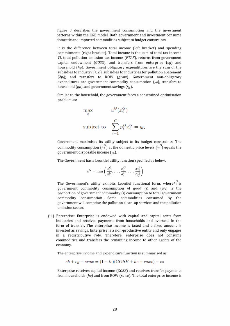
Figure 3: Investment/government flowchart of the economy
19 Subsidy payments are negligible in New Zealand, according to SAM outlined in section 3 of this report.
28
Figure 3 describes the government consumption and the investment patterns within the CGE model. Both government and investment consume domestic and imported commodities subject to budget constraints.
It is the difference between total income (left bracket) and spending commitments (right bracket). Total income is the sum of total tax income
TI, total pollution emission tax income (PTAX), returns from government
capital endowment (GOSG), and transfers from enterprise (eg) and
household (hg). Government obligatory expenditures are the sum of the
subsidies to industry (j, Zj), subsidies to industries for pollution abatement
(Zpj); and transfers to ROW (grow). Government non-obligatory expenditures are government commodity consumption (yG), transfers to
household (gh), and government savings (sg).
Similar to the household, the government faces a constrained optimisation
problem as:
Government maximises its utility subject to its budget constraints. The
commodity consumption ( ) at the domestic price levels ( ) equals the
government disposable income (yG).
The Government has a Leontief utility function specified as below.
The Government’s utility exhibits Leontief functional form, where is
government commodity consumption of good (i) and (aGi) is the proportion of government commodity (i) consumption to total government
commodity consumption. Some commodities consumed by the
government will comprise the pollution clean-up services and the pollution
emission sector.
(iii) Enterprise: Enterprise is endowed with capital and capital rents from industries and receives payments from households and overseas in the
form of transfer. The enterprise income is taxed and a fixed amount is
invested as savings. Enterprise is a non-productive entity and only engages
in a redistributive role. Therefore, enterprise does not consume
commodities and transfers the remaining income to other agents of the economy.
The enterprise income and expenditure function is summarised as:
Enterprise receives capital income (GOSE) and receives transfer payments
from households (he) and from ROW (rowe). The total enterprise income is
29
taxed at rate (te) and investment (es) is made as savings. The remaining
income is paid to households (eh), government (eg), and ROW (erow).
It is important to note that the flows by the enterprise can be redistributed
to other agents. In this situation the enterprise is removed from the CGE model, reducing the model’s complexity.
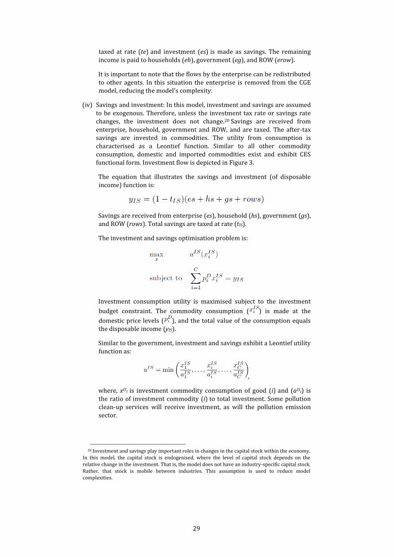
(iv) Savings and investment: In this model, investment and savings are assumed
to be exogenous. Therefore, unless the investment tax rate or savings rate
changes, the investment does not change.20 Savings are received from
enterprise, household, government and ROW, and are taxed. The after-tax savings are invested in commodities. The utility from consumption is
characterised as a Leontief function. Similar to all other commodity
consumption, domestic and imported commodities exist and exhibit CES
functional form. Investment flow is depicted in Figure 3.
The equation that illustrates the savings and investment (of disposable income) function is:
Savings are received from enterprise (es), household (hs), government (gs),
and ROW (rows). Total savings are taxed at rate (tIS).
The investment and savings optimisation problem is:
Investment consumption utility is maximised subject to the investment
budget constraint. The commodity consumption ( ) is made at the
domestic price levels ( ), and the total value of the consumption equals the disposable income (yIS).
Similar to the government, investment and savings exhibit a Leontief utility
function as:
,
where, xISi is investment commodity consumption of good (i) and (aISi) is
the ratio of investment commodity (i) to total investment. Some pollution clean-up services will receive investment, as will the pollution emission
sector.
20 Investment and savings play important roles in changes in the capital stock within the economy.
In this model, the capital stock is endogenised, where the level of capital stock depends on the
relative change in the investment. That is, the model does not have an industry-specific capital stock.
Rather, that stock is mobile between industries. This assumption is used to reduce model
complexities.
30
2.4.5 The relationship between household income and tax
Household income comes from the sale of people’s labour, net of paying income tax to the government. The household also receives environmental
compensation from firms and household subsidy payments from the
government. Each level of consumption requires some mix of pollution emission
or pollution clean-up services. Central and local governments have several
sources of income, and central government receives tax income from the pollution emission, the income tax revenue from the households, indirect tax,
and tariffs.
2.4.6 Trade with the rest of the world
We differentiate the domestic goods supplied to the domestic market from the
goods for trade and treat them as imperfect substitutes. Without this assumption,
either domestic or imported commodities with the lowest price will be
consumed. Similarly, the commodities will be sold either entirely domestically or
entirely exported depending on which market offers higher price. This result is due to price being the main determinant of demand in CGE models. To model
consumption of domestically produced and imported commodities, a CES type
function that aggregates imports and domestic sales into a composite good is
used. The sectoral output is defined as a CET function combining exports and
domestic sales of output. World market prices are exogenously given and the Armington approach illustrates reactions on the markets to changes in domestic
prices. 21 The balance of payment constraint (warranted through flexible
exchange rate) incorporates the benchmark trade surplus or deficit.
The equation that provides the CET export function is:
Domestic commodity production output (xPi) of commodity (i) is allocated to
exports (xXi), and domestic consumption (xDi), as dictated by CET elasticity (ρx)
and share (γi). Similar to household CES function, commodities become more
substitutable as ρx → ∞ and become complements as ρx → 0.
The export and domestic ratio function is given by this equation:
The optimal ratio between exports and domestic sale is given by export price (pXi)
and domestic price (pDi) of commodity (i).
The CES import function is specified as:
21 The Armington model assumes that a type of commodity produced by an economy is an
imperfect substitute of the same type of commodity produced by a different economy. This leads to consumers demanding the commodity from both economies and optimising their consumption patterns based on the price difference between the commodity from different economies and the magnitude of imperfect substitutability between the commodity. For example, imported vehicles from Japan and Germany are perceived as different but substitutable. As such, both are consumed despite the price difference.
31
Domestic commodity consumption (xCi) of commodity (i) comes from either
imports (xMi) or domestic output (xDi), depending on CES elasticity (ρm) and
share (τi). Similar to the household CES and export CET function, commodities
increasingly become substitutes as ρm → ∞ and become complements as ρm →
0.
The import and domestic ratio is given by:
Similar to exports, the optimal ratio between imports and domestic commodities
is given by import price ( ), and domestic price ( ) of commodity (i).
2.4.7 Market clearing and model closure
Equilibrium conditions have demand and supply of goods equal to each other as
is the case for the demand and supply of factors of production. Market clearing
equations describe this. The model has short-run and long-run macro closures.
Using an appropriate closure rule is very important as different closure rules
give very different results. To be consistent with most other CGE models, the
closure rule used in this report follows the standard neo-classical, short-run and long-run definition. Consequently, we closely follow the MONASH/ORANI model.
The main assumptions are that, in the short-run, the total amount of capital and
wage rate are exogenous and fixed. Yet the return to capital and the total amount
of labour are endogenously determined within the model. Under the long-run
closure rule, the total combined amount of capital and wage rate are taken to be endogenous while the return to capital and the total amount of labour are
exogenous and fixed. Therefore, the model behaves differently in the short run
than in the long run.
Changes in any exogenous variables will be zero unless exogenous shocks are
introduced. Conversely, this means that any variables that we can introduce exogenous shocks into will be exogenous variables. Important exogenous
variables in the model are tax rate, production technology, and savings rate.
2.4.8 Numerical specification of the model
To correctly specify the parameters of the model, the calibration approach is
adopted. The SAM approach is taken to adopt a consistent database for
calibration. We extend the traditional SAM to include regional information when
we build a multi-regional SAM based on the national SAM. This allows us to
capture the inter-regional transactions and contributions of each agent. The data that forms the basis of the SAM will be obtained from the latest supply-use tables
and national accounts published by Statistics New Zealand. The numerical
specifications of the model and how the SAM is built are discussed in greater
detail in section 3 of this report.
32
2.5 Incorporating the policy instruments for managing the quality of fresh water
The CGE model outlined in the previous section can be used to assess the
economic impacts of implementing various freshwater policy instruments.
Further, the model specifications are flexible and can be easily modified to suit
other types of policy instruments (e.g., setting limits for carbon emissions). Even
so, as the CGE model contains vast amounts of variables and links within the economic system, each policy instrument is likely to have a different method of
application into the CGE model.
Broadly, as noted earlier, the instruments can be applied within the model by
changing exogenous variables and/or setting up endogenous variables
depending on how the instrument affects the economic system. Therefore, setting up the model for an economic impact assessment of an instrument policy
requires a preliminary assessment of how the instrument affects the economy.
For input into this study, the Auckland Council Research and Evaluation Unit
(RIMU) provided a list of freshwater instruments for economic modelling (see
Appendix A to this report). Broadly, the three types of instrument options are spatial, non-spatial and consents/permits, while four instruments adhere to the
NPS-FM. The next subsection outlines examples of how to apply two22non-
spatial instruments that adhere to the NPS-FM and how to apply a hypothetical
social value instrument into the CGE model.
2.5.1 Freshwater limits
Under the policy instrument on freshwater limits, available freshwater is
constrained to meet the objective of good-quality fresh water. It is important to
note that the instrument is not a direct cap on the available fresh water within the economy as the pollutant emission levels are different depending on the
industry or consumer who uses it. As such, the constraint will change the
composition of the industrial outputs as well as consumption compared to the
base case. In addition, investment in abatement technology can alter the ratio of
pollutant emissions to output from different sectors of the economy.
Therefore, the limit of freshwater quality, or total pollutant emission levels
within the CGE framework, is set as an exogenous variable that limits the
production of the pollution commodity. That is, assuming a plentiful supply of
fresh water, total emissions must be less than equal to a set limit. This constraint
enters into the CGE model as:
where, xP is a pollutant emission good (P) and FL is an exogenous freshwater quantity limit measured in quantity of pollutant emission goods.
In addition, if the model includes fresh water as a factor of production, the quantity of fresh water supplied enters into the model as an endogenous variable that is a function of the former exogenous variable FL. Specifically, FWS
22 Two instruments were excluded: (i) spatial instrument involves setting up a Freshwater
management Unit (FMU); and (ii) in-stream value is the instrument that defines the limit settings for
freshwater quality.
33
is a variable of an endogenous supply of total fresh water subject to a constraint xP which equals FL.
2.5.2 Prioritising how fresh water is allocated
In the policy instrument ’freshwater allocation in order of priority’, the how
fresh water is allocated is based on a priority of: (i) health and wellbeing requirements for humans and animals; then (ii) economic, technical and
dynamic efficiency, and emergency shortage. Specifically, the priority of each
freshwater user in the economy is based on the priority target in turn, where the
user with a higher priority is allocated before the user with a lower priority. This
can be modelled within the CGE model using a set of constraints:
where u is the order of priority (1 being the highest priority) allocated to all
freshwater users, (FWu) is a quantity of fresh water used by the prioritised users
(u), and FWSu is the total freshwater quantity available to those users (u).
2.5.3 Incorporating social value into the model
Social value instruments in freshwater management can specifically consider
community, cultural, traditional Māori uses, environmental and aesthetics values.
Although economic values drive the CGE model, the non-economic values can be included in the model once those values are converted into the monetary (ie,
numerical) values used within the model. In turn, these values can be included
directly in the utility maximisation function, where the model calculates the
optimal trade-off level between economic and non-economic values.
Suppose the non-economic values are mainly considered by households. The household utility maximisation problem is then set out as:
In this example, households face a consumption decision where utility is a function of consumption of commodities and social value (SV). The decision is
now a maximisation problem subject to its budget constraints and the SV, which
is a function of xP.
2.6 Development programme for building an integrated model
To adhere to the National Policy Statement for Freshwater Management (NPS-
FM), Auckland Council is undertaking research to understand the channels of water pollution and measure quantities of pollutants emitted within the region.
The models used within the research are based on freshwater models, and
researchers were interested in incorporating the CGE model and, in particular,
building an integrated model. Such models may answer a detailed spatial level
34
economic and physical consequences associated with limit setting policies and
significantly increase the depth of the research currently undertaken. As far as
the author is aware, there are two water management researches23 undertaken
in New Zealand which involves building an integrated model with a CGE based economic module.
Even so, building an integrated model is an enormous undertaking where substantial time and expert inputs from relevant fields are required. In addition, researchers within the council indicated a CGE model, such as the one proposed here, can be used beyond the freshwater management studies currently undertaken. But any future research should adhere to other aspects of the National Policy Statements.
In light of this, the proposed CGE model should have future use in mind and must be able to be integrated into other models. At this stage it is not feasible to build
a development programme for a CGE model meeting the requirements noted
above. This is because outlining such a programme would require an extensive
scoping study involving various potential council users of the model.
Broadly, the development process for the CGE model focused on freshwater quality will have three major stages.24
1. Build the modules for use within the CGE model: The main objective of
this stage is to build modules to be used within the CGE model, where
those modules simulate emission channels as a consequence of production.
This includes abatement and consumption activities within the economy. We were unable to find any research within New Zealand on a water
quality model being endogenously integrated into an economic model. We
expect that developing the water quality module will take a large share of
resources (time and people).
2. Modify and update the CEU sub-regional housing to: This stage
involves modifying and updating the specifications of the current CEU sub-regional housing CGE model to accommodate the module built in the first
stage. The key tasks in this stage are to identify and specify the sub-
regional areas, production sectors, and economic agents that the CGE
model will model. Subsequently, appropriate SAM corresponding to the
specification needs to be built.
Finally in this stage, the model formulation and mathematical functions of
CEU sub-regional housing CGE model will be modified to match the
identified specification. The challenging aspect of this stage is to build the
underlying SAM, as this involves intensive data mining. The data required
to build an accurate sub-regional, level-based economic database (i.e., SAM)
23 (1) Southland Regional Council is developing an integrated CGE model to assess the economic implications of water allocation and limit-setting initiatives in the Southland region. Further information is in Stage 1 of this report. (2) Smart Models for Aquifer Characterisation is a multi-year research programme funded by the Ministry of Business, Innovation and Employment. In that programme, ground and surface water models, a land-use model, and a CGE-based economic model are integrated to support decisions on risk. The key focus of the research is to develop a simple model design that is easily incorporated into decision making. The research is co-funded by Environment Southland, Environment Waikato and the Greater Wellington Regional Council.
24 An important part of a research programme is a feasibility and scoping study. This part is normally included as a first stage of a research programme. However, this study forms part of the feasibility and scoping study for the proposed study and so the development programme in this report does not include a separate feasibility and scoping study.

35
to be used within the CGE model is lacking. Even at the regional level, only
a small amount of data is available to test in the technical estimation
methods needed to build SAM. Section 3 of this report includes a detailed
technical methodology for building SAM.
3. Incorporate the CGE model with the modules for managing
freshwater quality: The key tasks in this stage are to integrate the CGE
model built in stage 2 with the modules built in stage 1, to calibrate the
model, and to test the robustness of the results. Such a calibration exercise
(where the model is tested and fitted against real-world data) makes the model more reliable and the results more robust.
In addition, the estimation and testing of economic model parameters (e.g.,
elasticities used within the CGE function) will be run alongside the
calibration process. Finally, the final output will be promoted in
workshops and conferences, with a written technical document and practitioner’s guide.
We estimate the programme will take about 12 months, with each stage taking
about 4 months.. The time needed depends on the availability of council staff and,
from consulting with the council, we expect the full study will involve an initial
scoping study and then modification of the CGE model when required.
2.6.1 The four groups within the project team
The programme’s project team has four major groups.
1. A Technical Advisory Group (TAG) is expected to provide broad advice to, and assist with, the overall direction of the project. This will ensure the
final outcome of the programme aligns with the requirements of the
council and other local and central government agencies.
2. A management group will assist a research team during the project, by
liaising with different departments within the council, TAG and the peer reviewer. It will also help to run workshops and participate in promoting
the programme. The management team is also expected to take part within
TAG.
3. A peer reviewer will be heavily involved throughout the project, helping
with technical aspects of the proposed model. This will ensure that any problems are addressed early in the project. Each stage has six major peer
review points (in two steps). The technical methods will be specified and
peer reviewed at the start of each stage. The final output of each stage will
be peer reviewed at the end of that stage.
4. A research team will be responsible for conducting the programme. Although it is expected that the development process will be
straightforward, implementing and testing the robustness of the
freshwater-quality module will require substantial technical expertise. In
particular, the proposed model includes endogenous freshwater-quality
modules not previously undertaken in New Zealand.
Compared to researchers with skills in other economic impact assessment
methods, (i.e., CBA and IO), considerably fewer researchers within
New Zealand have skills in the CGE model. So the biggest barrier to the

36
development process will be acquiring skilled CGE practitioners capable of
building and implementing the freshwater-quality module.
2.6.2 The project’s Five key deliverables
The development programme has five key deliverables.
1. The module for managing the quality of fresh water: The modules built
in Stage 1 will be able to model channels of water pollutant emissions in
economic production, consumption, and abatement. Auckland Council can apply these modules, as can other local councils, into an economic model
used to calculate the quantity of pollutant emissions from the economy. In
addition, the modules can be modified to measure pollutants other than
water.
2. The generic CGE model: Stage 2 will involve building a generic multi-regional CGE model capable of handling regional and sub-regional spatial
areas. Although, at first, this model will be used for the Auckland region, it
can be run for other regions. In addition, the generic structure of the model
will allow easy implementation to future policy studies and to any
economic module within an integrated model (e.g., the EIA of setting limits for carbon emissions).
3. CGE model for managing the quality of fresh water: The CGE model to
assess economic implications of the water quality limit setting initiatives
will be created. This model can be used as a stand-alone tool or as a part of
integrated model.
4. Technical documentation and a practitioner’s guide: Key outputs of
the development programme will be technical documentation and a
practitioner’s guide. The technical documentation will provide full
technical details on the methodology, procedures and data used within the
programme. It is envisioned that the researchers will be able to use the document to develop similar models in the future. The practitioner’s guide
will provide details on how to use the built model and guidelines on how
to use the CGE model to conduct EIAs.
5. Workshops and presentations: Workshops on the built model will be
run within the council and in other government agencies to promote and inform researchers. The project’s research team will also participate in
conferences and present the model to inform wider audiences throughout
New Zealand.
2.6.3 Risks to completing the project successfully
The development programme faces several possible risks.
1. Technical complexity of the model: The CGE model and freshwater-
quality modelling proposed in this study is at the cutting edge of economic EIA. As such, building the model is highly technical and the research team
will most likely face technical difficulties during the development
programme. As noted above, New Zealand has only a handful of CGE
experts. Even so, a number of private organisations and academics own
37
and operate CGE models within New Zealand. As such, technical difficulties
can be mitigated by seeking expert advice.
2. Loss of key members of the research team: Losing key team members is
a well-known risk involved with a long-term research programme such as this. As to the first risk, the technical complexity of the CGE model adds to
this second risk as New Zealand has only a limited number of researchers
with the necessary skills. Also, the key objective of the development
programme is increasing CGE capabilities within the council. The loss of
any key member of the research team will hinder us in achieving this objective.
To mitigate the risk, the CGE model will be based on a standard CGE
structure built on a widely used programme code. This ensures that the
model is easily transferable and people will not need much time to become
familiar with it.
3. Unavailability of key data to populate and check the model: The
robustness of an applied model depends greatly on having accurate data.
Building the CGE model will require detailed regional economic data and
sub-regional data. Within New Zealand, the data required to build a
detailed regional and sub-regional housing CGE model is lacking. So CGE modellers will use numerical estimation methods to build the underlying
data.25 In addition, water accounts and pollution data for Auckland are still
being developed, creating the risk that data is not available before this
development programme starts.
Two actions can mitigate this risk of unavailability risk: use an established method to numerically estimate unavailable data; and then update the
data as unavailable data becomes available.
4. Project scope creep: As noted earlier, researchers within the council
were interested in using the proposed CGE model for various policy issues
and in applying the model as an economic module within an integrated model. This means the scope of the development programme may expand
to include other issues. This would lead to delays in delivering the model
within the set timeframe.
In response to this risk, the model will be built in two stages: (i) the base
CGE model; and (ii) the base CGE model expanded to incorporate the freshwater-quality module.
25 CGE modellers in New Zealand are not the only modellers to have little available data to build
SAM. CGE modellers in most other countries have the same problem. The SAM data construction
method outlined in this report also uses numerical estimation methods. See section 3 for further
details.
38
3 Stage 3: Gap analysis on data requirements
and the value of the study
In general, building a CGE model framework involves analysing the transactions
of numerous economic agents.26 One advantage of the modern CGE modelling
based on Johansen (1960)[21] is that it is based on national accounts data
publicly available for most countries. The downside of this approach is that the
same data used to estimate the parameters to build the model are used to provide the benchmark for the model.
This section discusses the data required to model the sub-regional CGE model
with the freshwater module. Subsection 3.1 provides an overview of the data
requirements, subsection 3.2 describes New Zealand National Social Accounting
Matrices, subsection 3.3 outlines a full data construction methodology, and subsection 3.4 lists the data requirements for incorporating a freshwater module.
3.1 Overview of the data requirements
3.1.1 Social accounting matrix
Most economic impact analyses involve using some form of economic data in
building and estimating parameters for the models. The National Accounts (NAs) 27 prepared by Statistics New Zealand (SNZ) provide a good source of economic
data for creating a snapshot of the economy at a given point in time. In addition,
other accounts, such as the Household Economic Survey [50], Institutional
Sector Accounts (Sector Accounts) [53], Harmonised System for Trade [52], can
be used to supplement the NAs to provide a more complete picture of the transactions made by the main agents28 in an economy.
The economic information contained in the aforementioned tables and accounts
noted in the above paragraph can appear in many forms. In applying the CGE
modelling, which is the proposed methodology in this report, economic data are
best represented in a matrix form. This is because the matrix form can represent the market-clearing concept in an intuitive way. The concept of equilibrium and
market clearing is fundamental to most economic modelling. As the equilibrium
identities dictate the total supply to equal use or input to output or income to
expenditure, the same concept can be applied in summarising the NAs.
In this report, the data requirements to build a comprehensive sub-regional housing model are discussed in the context of the following three matrices that
summarise the NAs: (1) the National Social Accounting Matrix (NSAM); (2) the
Multiregional Social Accounting Matrix (RSAM); and (3) the Sub-regional Social
Accounting Matrix (SSAM).
26 A CGE model environment may often involve households, producers, commodities, industries,
government and others, which can lead to an estimation of parameters that is data intensive. 27 Statistics New Zealand follows the convention as set out in the United Nations System of
National Accounts (1993)[59]. 28 An agent in the context of CGE modelling means any entity (such as households, governments)
engaged in economic activities.
39
3.1.2 Spatial economic data
The main spatial economic dataset used in this analysis is New Zealand Business Frame (BF) [51]. This dataset contains employment by industries in 6 Digit
ANZSIC06. The data is used in conjunction with the meshblock data from the
2013 Census (Meshblock 2013). Meshblock 2013 is a geographical division of
New Zealand land mass relative to categorical and quantitative variables such as
population density and types of land use. Each meshblock in a BF dataset contains industry employment information. The employments are further
categorised into New Zealand Employment Counts (EC) and Geographical Units
(GU). Our main data of interest is EC.
The dataset can be further aggregated into:
• 6 Digit ANZSIC Classifications into 106 Supply and Use table industries
• Meshblock 2013 area into FMUs and the ROW.
Aggregation of the dataset is possible as the original dataset contained more
than 40,000 meshblocks and 500 industry classifications. That dataset is too
detailed for our purpose. So each land area of interest will be FMU areas within Auckland and ROW, which contains ECs by 106 industries from the Supply and
Use table.
3.2 New Zealand National Social Accounting Matrices
The use of SAMs in economic impact analyses is well-supported in literature and
is the main source of data for CGE modelling. Even so, building a SAM can be
costly due to the substantial time and effort required to obtain and analyse the appropriate economic data. Accordingly, few examples of SAMs are built for
New Zealand at the national and regional levels. One early example of updating
the New Zealand SAM is featured in Zhang et al. (2008)[63]. In the report, the
authors created the National Supply-Use Table for 2003 based on the 2003 NAs
and the existing 2002-2003 National Supply-Use Table (NSUT).
The NSAM and RSAM are then built based on the NSUT and the regionalised
NSUT. The report well demonstrates the substantial effort required to produce
an update of SAMs. The same set of NSUT published for the 2002–2003 year has
been used in other studies. Most notably, a series of studies published by private
consulting firms, the New Zealand Institute of Economic Research (NZIER) and Infometrics use the 2002–2003 NSUT to evaluate the impact of carbon emission
trading schemes in New Zealand.29 30
A more recent example of NSAM and RSAM built for the New Zealand economy is
presented in Smith et al. (2015) [44] where the authors extend the approach
29 Seven studies, published by Infometrics (2007, 2008) [19], NZIER (2008) [37], NZIER and
Infometrics (2009, 2011) [38], [39], Landcare Research (2008) [13] and Lennox and van Nieuwkoop (2010) [26], apply the 2002–2003 NSUT in a CGE setting to study the impact of carbon emission trading schemes in New Zealand.
30 We were not able to obtain information on the detailed mathematical formulation used for the CGE models and the underlying SAMs that NZIER and Infometrics use. This report assumes that, given the models that NZIER use are mainly based on the MONASH/ORANI specification their SAM would be built like the Australian SAM. However, it is unclear how the differences in treating and disclosing data from SNZ and its Australian counterpart are accounted. It is also unclear how differences in the transactional characteristics of industry sectors between the two countries are accounted.
40
outlined in Zhang et al. (2008) [63] to build the updated NSAM and RSAM using
the 2006–2007 NSUT. Robson (2012) [42] provides a description of a prototype
RSAM for 25 industry types and 5 regions in New Zealand. In the context of
managing the quality of fresh water at the regional level, Market Economics has been involved in two separate studies using the CGE model framework.
The first study is Southland Regional Council’s integrated CGE model to assess
the economic implications for the Southland region of water allocation and
initiatives that set limits.31
The second study is Smart Models for Aquifer Management as part of a multi-year MBIE funded research programme, where groundwater and surface water
models, land use model, and a CGE based economic model are integrated to
support decision making based on risk.
Although numerous RSAMs are created by research organisations throughout
New Zealand, it is hard to know whether these will be available for council to use. As such, the next section of the report outlines a detailed method of building
NSAM, RSAM and sub-regional SAM. Broadly, the method is a mix of
methodology used by Market Economics Ltd and The Enormous Regional Model
(TERM) database construction methodology outlined in the paper by Mark
Horridge from the Centre of Policy Studies (CoPS), based at Victoria University in Melbourne.
3.3 Building the social accounting matrices for the sub-regional model
The sub-regional housing model will be based on the latest NSUT available from
SNZ. The latest tables that SNZ released in April 2016 are based on the 2013
financial year. The NSUT outlines the input requirements, final input demand
and the final output production by 106 industries of 201 commodities. The 2013
NSUT will form the basis for building the NSAM, along with the RSAM and SSAM.
Other data sources, such as the New Zealand Census and AgriBase, will be used to supplement the requirement for employment and population data.
This section briefly discusses the main components and data requirements for building each SAM.
3.3.1 The 2013 National Social Accounting Matrix
The 2013 NSAM will be based on the data contained within the 2013 NSUT. The NSAM will condense the information from the 106 industries and 201
commodities contained in the 2013 NSUT. The condensed matrix will focus on
industries, commodities, labour and capital32 as factors of production, an
enterprise, a household, local and central government, direct and indirect taxes,
savings/investment and ROW.
An example of NSAM is illustrated in Figure4. As shown in the example, NSAM
features the main economic agents, their income and expenditure activities and
the total value of those activities. The economic agents modelled in the NSAM are
31 See Stage 1 of this report for further information about Southland Regional Council’s initiative. 32 Capital will contain physical capital and land as its two main components, and so incorporate
the land use information into the sub-regional housing model.
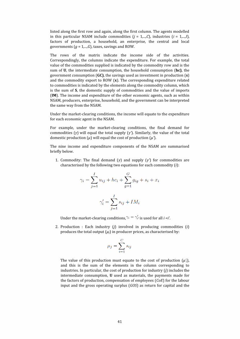
41
listed along the first row and again, along the first column. The agents modelled
in this particular NSAM include commodities (j = 1,...,C), industries (i = 1,...,I),
factors of production, a household, an enterprise, the central and local
governments (g = 1,...,G), taxes, savings and ROW.
The rows of the matrix indicate the income side of the activities.
Correspondingly, the columns indicate the expenditure. For example, the total
value of the commodities supplied is indicated by the commodity row and is the
sum of U, the intermediate consumption, the household consumption (hc), the
government consumption (GC), the savings used as investment in production (s) and the commodity export to ROW (x). The corresponding expenditure related
to commodities is indicated by the elements along the commodity column, which
is the sum of S, the domestic supply of commodities and the value of imports
(IM). The income and expenditure of the other economic agents, such as within
NSAM, producers, enterprise, household, and the government can be interpreted the same way from the NSAM.
Under the market-clearing conditions, the income will equate to the expenditure
for each economic agent in the NSAM.
For example, under the market-clearing conditions, the final demand for
commodities (γ) will equal the total supply (γ’). Similarly, the value of the total domestic production (µ) will equal the cost of production (µ’).
The nine income and expenditure components of the NSAM are summarised
briefly below.
1. Commodity: The final demand (γ) and supply (γ’) for commodities are
characterised by the following two equations for each commodity (i):
Under the market-clearing conditions, is used for all i =i’.
2. Production : Each industry (j) involved in producing commodities (i) produces the total output (µj) in producer prices, as characterised by:
The value of this production must equate to the cost of production (µ’j), and this is the sum of the elements in the column corresponding to
industries. In particular, the cost of production for industry (j) includes the
intermediate consumption, U used as materials, the payments made for
the factors of production, compensation of employees (CoE) for the labour
input and the gross operating surplus (GOS) as return for capital and the
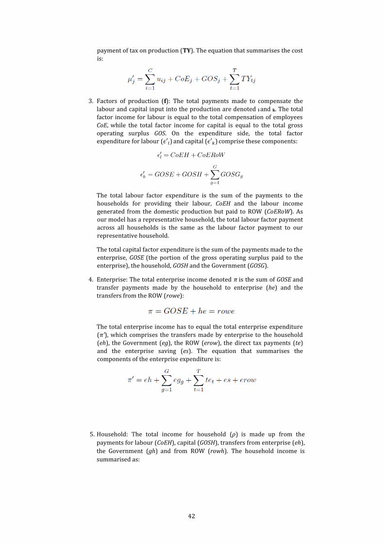
42
payment of tax on production (TY). The equation that summarises the cost
is:
3. Factors of production (f): The total payments made to compensate the
labour and capital input into the production are denoted l and k. The total
factor income for labour is equal to the total compensation of employees
CoE, while the total factor income for capital is equal to the total gross
operating surplus GOS. On the expenditure side, the total factor expenditure for labour (𝜖′𝑙) and capital (𝜖′𝑘) comprise these components:
The total labour factor expenditure is the sum of the payments to the
households for providing their labour, CoEH and the labour income
generated from the domestic production but paid to ROW (CoERoW). As our model has a representative household, the total labour factor payment
across all households is the same as the labour factor payment to our
representative household.
The total capital factor expenditure is the sum of the payments made to the
enterprise, GOSE (the portion of the gross operating surplus paid to the enterprise), the household, GOSH and the Government (GOSG).
4. Enterprise: The total enterprise income denoted π is the sum of GOSE and
transfer payments made by the household to enterprise (he) and the
transfers from the ROW (rowe):
The total enterprise income has to equal the total enterprise expenditure
(π’), which comprises the transfers made by enterprise to the household
(eh), the Government (eg), the ROW (erow), the direct tax payments (te)
and the enterprise saving (es). The equation that summarises the
components of the enterprise expenditure is:
5. Household: The total income for household (ρ) is made up from the
payments for labour (CoEH), capital (GOSH), transfers from enterprise (eh),
the Government (gh) and from ROW (rowh). The household income is
summarised as:
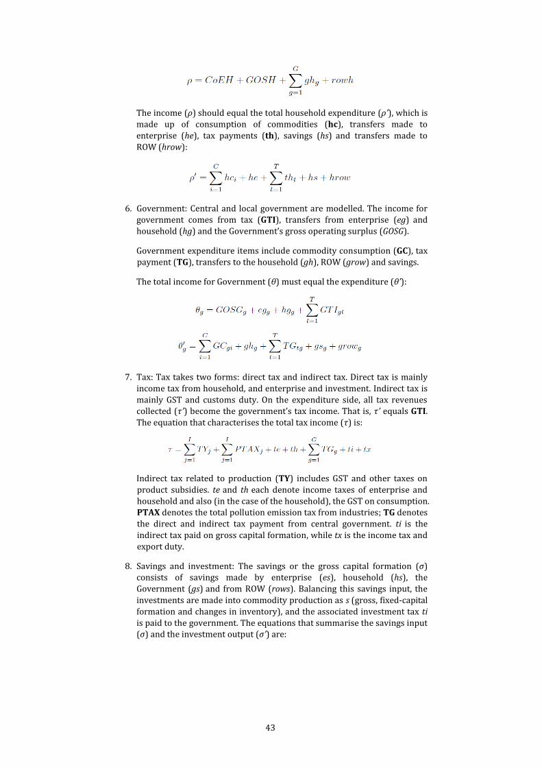
43
The income (ρ) should equal the total household expenditure (ρ’), which is
made up of consumption of commodities (hc), transfers made to
enterprise (he), tax payments (th), savings (hs) and transfers made to
ROW (hrow):
6. Government: Central and local government are modelled. The income for government comes from tax (GTI), transfers from enterprise (eg) and
household (hg) and the Government’s gross operating surplus (GOSG).
Government expenditure items include commodity consumption (GC), tax
payment (TG), transfers to the household (gh), ROW (grow) and savings.
The total income for Government (θ) must equal the expenditure (θ’):
7. Tax: Tax takes two forms: direct tax and indirect tax. Direct tax is mainly
income tax from household, and enterprise and investment. Indirect tax is
mainly GST and customs duty. On the expenditure side, all tax revenues collected (τ’) become the government’s tax income. That is, τ’ equals GTI.
The equation that characterises the total tax income (τ) is:
Indirect tax related to production (TY) includes GST and other taxes on
product subsidies. te and th each denote income taxes of enterprise and
household and also (in the case of the household), the GST on consumption. PTAX denotes the total pollution emission tax from industries; TG denotes
the direct and indirect tax payment from central government. ti is the
indirect tax paid on gross capital formation, while tx is the income tax and
export duty.
8. Savings and investment: The savings or the gross capital formation (σ) consists of savings made by enterprise (es), household (hs), the
Government (gs) and from ROW (rows). Balancing this savings input, the
investments are made into commodity production as s (gross, fixed-capital
formation and changes in inventory), and the associated investment tax ti
is paid to the government. The equations that summarise the savings input (σ) and the investment output (σ’) are:
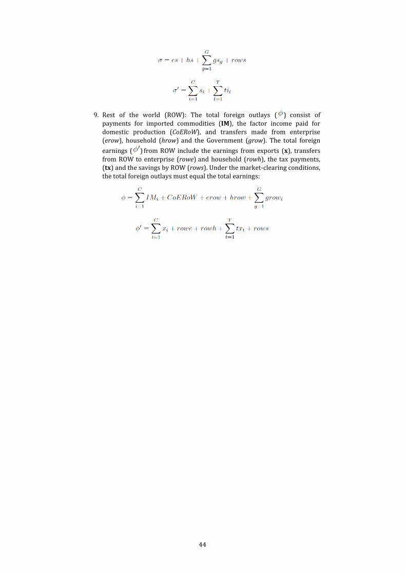
44
9. Rest of the world (ROW): The total foreign outlays ( ) consist of
payments for imported commodities (IM), the factor income paid for
domestic production (CoERoW), and transfers made from enterprise (erow), household (hrow) and the Government (grow). The total foreign
earnings ( ) from ROW include the earnings from exports (x), transfers
from ROW to enterprise (rowe) and household (rowh), the tax payments, (tx) and the savings by ROW (rows). Under the market-clearing conditions,
the total foreign outlays must equal the total earnings:
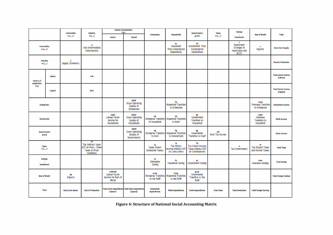
Figure 4: Structure of National Social Accounting Matrix
Data requirements for the National Social Accounting Matrix
The primary data source for NSAM is a national-level, input-output table. The latest available NSUT (published for the 2013 financial year) and the 2013 NAs
will be used to build the 2013 NSAM. The main data sources are:
• the National Supply Use (Input Output) Table for the year ended 2013
[48]
• Statistics New Zealand’s National Accounts (Income and Expenditure) for
the year ended 2013 [55].
To use the NSUT when building the NSAM, the total supply of each commodity in
the NSUT must equal the total use. Also, the total income of each industry must
equal the total expenditure. The row totals and the column totals differ slightly for the tables published by SNZ. An optimisation method is used to reduce the
difference within the target range before we can apply it to build the NSAM.33
The other data source required for building the NSAM is a series of tables
published as part of SNZ’S National Accounts (Income and Expenditure). The
following 13 tables are included in the Income and Expenditure account.
Table 1: National Accounts Income and Expenditure
Table 2.1 Producer enterprises sector accounts
Table 2.2 Private corporate producer enterprises and
producer boards sector accounts
Table 2.3 Private non-corporate producer enterprises
sector accounts
Table 2.4 Central government enterprises sector accounts
Table 2.5 Local government enterprises sector accounts
Table 2.6 Financial intermediaries sector accounts
Table 2.7 General government sector accounts
Table 2.8 Central government sector accounts
Table 2.9 Local government sector accounts
Table 2.10 Private non-profit organisations serving
households sector accounts
33 One commonly used method to balance the income and expenditure totals is a ‘least squares’
optimisation method. This method minimises the squared difference between the total and the
target value subject to the identified income and expenditure constraint. See Smith et al. (2015) [44]
for further detail.
47
Table 2.11 Households sector accounts
Table 2.12 Household final consumption expenditure
Table 2.13 Rest of world sector accounts
The complete set of data sources for each NSAM account is available in the Data
Sources for NSAM at Appendix B of this report.
3.3.2 The multi-regional Social Accounting Matrix
A regional-level SUT is required to build an RSAM. Ideally, the regional SUT
should be built from the ground up and based on information obtained from
each region. However, as detailed regional data is lacking, most RSAM are built
by regionalising a national-level SUT using various estimation methods.
The basic idea behind the estimation approach is to assume that the regional
account is a proportion of the national account. In addition, the regional accounts should sum up to the national account in a given year. For example, the regional
supply (Sr) can be estimated by αS, where α denotes a coefficient that gives the
regional share of the national output and S is the total national output. In other
words, say if Auckland is attributable for one quarter of the national financial
and banking services, then Auckland’s regional supply of financial and banking services is estimated to be one quarter of the national supply.
In practice, estimating this share coefficient can be difficult due to regional data
constraints. Further, the classification of the national output into 106 industries
and 201 commodities within the SUT framework means that some commodities
grouped together may differ greatly in how they are traded between regions.
In our report, we investigate the construction of RSUT and RSAM based on the
2013 NSUT and the Regional Gross Domestic Production (RGDP)[54] accounts
published by SNZ.34
Constructing the regional supply-use table
In this report, we outline the process of regionalising the NSUT into 15 regions
as defined in the RGDP accounts by SNZ. The following steps summarise the
main processes of building a RSUT.
1. Regional supply (Sr): The regional share of national supply of commodity i for industry j within region r is given by this equation:
34 Where available, more detailed regional data is incorporated to improve the estimates of share
coefficients. This may involve a non-numerical approach of making manual (possibly subjective)
adjustments based on additional research.
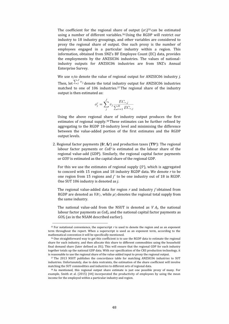
48
The coefficient for the regional share of output (orj)35 can be estimated
using a number of different variables.36 Using the RGDP will restrict our industry to 18 industry groupings, and other variables are considered to proxy the regional share of output. One such proxy is the number of
employees engaged in a particular industry within a region. This information, obtained from SNZ’s BF Employee Count (EC) data, provides
the employments by the ANZSIC06 industries. The values of national-industry outputs for ANZSIC06 industries are from SNZ’s Annual Enterprise Survey.
We use vj to denote the value of regional output for ANZSIC06 industry j.
Then, let denote the total industry output for ANZSIC06 industries matched to one of 106 industries.37 The regional share of the industry
output is then estimated as:
Using the above regional share of industry output produces the first
estimates of regional supply.38 These estimates can be further refined by
aggregating to the RGDP 18-industry level and minimising the difference
between the value-added portion of the first estimates and the RGDP
output levels.
2. Regional factor payments (flr, fkr) and production taxes (TYr): The regional
labour factor payments or CoEr is estimated as the labour share of the
regional value-add (GDP). Similarly, the regional capital factor payments
or GOSr is estimated as the capital share of the regional GDP.
For this we use the estimates of regional supply (Sr), which is aggregated to concord with 15 region and 18 industry RGDP data. We denote r to be
one region from 15 regions and j’ to be one industry out of 18 in RGDP.
One SUT 106 industry is denoted as j.
The regional value-added data for region r and industry j’ obtained from
RGDP are denoted as VArj’, while µrj’ denotes the regional total supply from the same industry.
The national value-add from the NSUT is denoted as V Aj, the national
labour factor payments as CoEj, and the national capital factor payments as
GOSj (as in the NSAM described earlier).
35 For notational convenience, the superscript r is used to denote the region and as an exponent
term throughout the report. When a superscript is used as an exponent term, according to the mathematical convention it will be specifically mentioned.
36 One straightforward way to get this coefficient is to use the RGDP data to estimate the regional
share for each industry, and then allocate this share to different commodities using the household
final demand share (later defined as DSi). This will ensure that the regional GDP for each industry
together totals up the national GDP data. With our specification of the CRS production technology, it
is reasonable to use the regional share of the value-added input to proxy the regional output. 37 The 2013 NSUT publishes the concordance table for matching ANZSIC06 industries to SUT
industries. Unfortunately, due to data restraints, the estimation of the share coefficient will involve
matching the SUT commodities and industries to different sets of regional data. 38 As mentioned, this regional output share estimate is just one possible proxy of many. For
example, Smith et al. (2015) [44] incorporated the productivity of employees by using the mean
income for the employed within a particular industry and region.

49
The labour and capital factor payments are then estimated using these two
equations:
In both equations, the term is the regional supply of industry j’ in
region r and denotes the value-added portion of the total regional
output by industry j’. Finally, is the labour share of the national value
added and is the capital share of the national value added.
The product taxes, TYr can be estimated once the commodity consumption
accounts are estimated in steps (3) to (9).39
3. Regional intermediate consumption (Ur): The estimate of regional
intermediate consumption (Ur) is derived in a number of stages. As in
step 1 above, the first estimates are produced and then refined depending
on what data is available. The regional intermediate consumption is
categorised into two types of commodities: the use of domestic commodity
(uD,ri,j) and imported commodities (uM,ri,j). The following share coefficients
are defined for estimating regional commodity use:
Here, the terms respectively denote the total national use of domestic commodity i by industry j and the total national use of imported
commodity i by industry j. The total national cost of production for
industry j is denoted as µ’j, while V Aj denotes the total national value-
added portion of the cost. That is, .
Using the above share coefficients, an estimate of domestic commodity use
in production for industry j in region r is:
Similarly, an estimate of imported commodity use in production for
industry j in region r is:
39 Product taxes are conventionally linked to commodities and not industry accounts as in NSUT. It
is possible to estimate the regional share of product taxes for each industry in the same way as the regional industry supply. Here, the product taxes are estimated using the estimates from the commodity account.

50
While no further adjustment is required for the estimates of imported
commodity use, the estimates of other commodity accounts derived in
steps 4 to 7 below can help to further refine the domestic commodity use
in production.
4. Regional household consumption (hcr): The regional household
consumption is estimated using a coefficient calculated as the region’s total household income as a proportion of the total national household
income. This is based on an assumption that those regions with higher household income consume higher shares of the national consumption. The following equations illustrate the derivation:
The NSUT provides the value of hcDi, the total national household consumption of commodities produced domestically, while hcMi is the total
national household consumption of imported commodities. The household
income share coefficient, Hr is calculated as:
Both the regional household income and the total national household income can be sourced from SNZ’s New Zealand Income Survey.
5. Regional investment in commodity (sr): As for regional household
consumption of commodities, the regional investment into commodities
can be estimated using the household income share coefficient (Hr). Again,
this is based on the assumption that those regions with a higher household income invest higher shares of the national commodity consumption. Both
the regional investment in domestic consumption and the imports are
calculated as:
Both the investment in domestic consumption and imports data are
available from NSUT.
6. Regional government consumption (GCr): For government g’s
consumption of commodity i in region r, the appropriate share coefficient
for each region is considered proportional to the regional population. That
is, the higher the population in a particular region, the higher the
government spending on consumption for that region.
This coefficient denoted as Pr is calculated as:
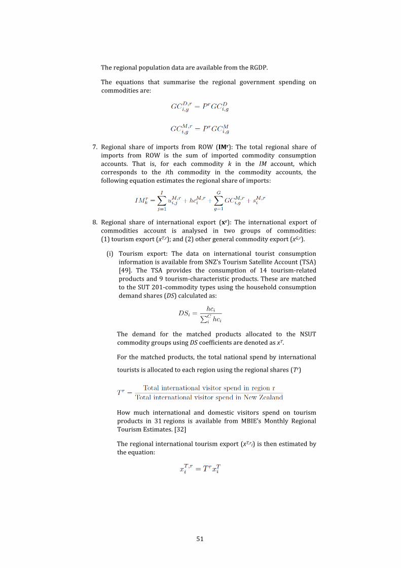
51
The regional population data are available from the RGDP.
The equations that summarise the regional government spending on
commodities are:
7. Regional share of imports from ROW (IMr): The total regional share of
imports from ROW is the sum of imported commodity consumption
accounts. That is, for each commodity k in the IM account, which corresponds to the ith commodity in the commodity accounts, the
following equation estimates the regional share of imports:
8. Regional share of international export (xr): The international export of
commodities account is analysed in two groups of commodities:
(1) tourism export (xT,r); and (2) other general commodity export (xG,r).
(i) Tourism export: The data on international tourist consumption
information is available from SNZ’s Tourism Satellite Account (TSA) [49]. The TSA provides the consumption of 14 tourism-related
products and 9 tourism-characteristic products. These are matched
to the SUT 201-commodity types using the household consumption
demand shares (DS) calculated as:
The demand for the matched products allocated to the NSUT
commodity groups using DS coefficients are denoted as xT.
For the matched products, the total national spend by international
tourists is allocated to each region using the regional shares (Tr)
How much international and domestic visitors spend on tourism
products in 31 regions is available from MBIE’s Monthly Regional
Tourism Estimates. [32]
The regional international tourism export (xT,ri) is then estimated by
the equation:
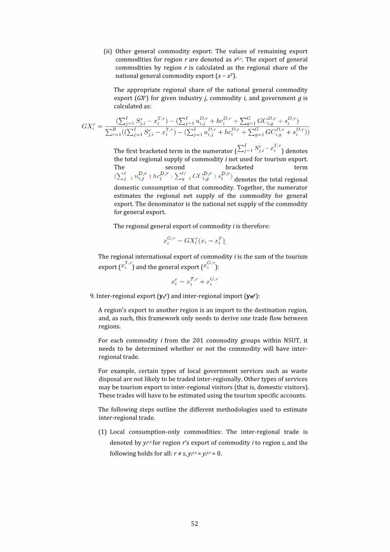
52
(ii) Other general commodity export: The values of remaining export
commodities for region r are denoted as xG,r. The export of general
commodities by region r is calculated as the regional share of the
national general commodity export (x − xT).
The appropriate regional share of the national general commodity
export (GXr) for given industry j, commodity i, and government g is
calculated as:
The first bracketed term in the numerator ( ) denotes the total regional supply of commodity i not used for tourism export.
The second bracketed term
denotes the total regional domestic consumption of that commodity. Together, the numerator
estimates the regional net supply of the commodity for general
export. The denominator is the national net supply of the commodity for general export.
The regional general export of commodity i is therefore:
.
The regional international export of commodity i is the sum of the tourism
export ( ) and the general export ( ):
9. Inter-regional export (yxr) and inter-regional import (yMr):
A region’s export to another region is an import to the destination region, and, as such, this framework only needs to derive one trade flow between
regions.
For each commodity i from the 201 commodity groups within NSUT, it
needs to be determined whether or not the commodity will have inter-
regional trade.
For example, certain types of local government services such as waste disposal are not likely to be traded inter-regionally. Other types of services
may be tourism export to inter-regional visitors (that is, domestic visitors).
These trades will have to be estimated using the tourism specific accounts.
The following steps outline the different methodologies used to estimate
inter-regional trade.
(1) Local consumption-only commodities: The inter-regional trade is
denoted by yir,s for region r’s export of commodity i to region s, and the
following holds for all: r ≠ s, yir,s = yis,r = 0.

53
(2) Inter-regional tourism: For the 14 tourism-related products and 9
tourism-characteristic products, TSA provides the spend by domestic
visitors. As for the estimation of international tourism export, the
tourism products (as defined in TSA) are matched to NSUT 201-commodity using the household demand shares (DSi). To estimate the
inter-regional tourism ( ), the values used are:
The inter-regional tourism is then estimated as:
(3) National supplier commodity: For commodities (such as electricity) that all users trade off the national grid, it is appropriate to estimate
the region’s export to other regions as its share of total national
production of that commodity.40 One example would be if the Waikato
region produces one-quarter of the total electricity, and then the
region exports one-quarter of its national electricity output to all other regions. Other examples of national supplier commodities include the
central government services, such as civil construction and military
services.
(4) All other commodities: The inter-regional trade for all other
commodities are estimated using the Gravity Model method as outlined in Smith et al. (2015) [44]. Initially developed to model
international trade flows, the model has been applied in Input-Output
and SUT analyses to model inter-regional trade flows. The basic
specification of the inter-regional trade (yir,s) is as a function of the
supply of commodity i by the exporting region, the use of that commodity by the importing region, and the trade impedance factor
denoted as q. The inter-regional trade is then estimated as:
,
where:
denotes the region r’s total domestic supply of i
denotes the total domestic supply of i by all regions
40 Calculating a regional share of electricity import and export is difficult due to the uniqueness of
the operation mechanism of the electricity market. As such, we have opted to use a simple approach.
Alternatively, the Gravity Model method as outlined in Smith et al. (2015) [44] can be used.
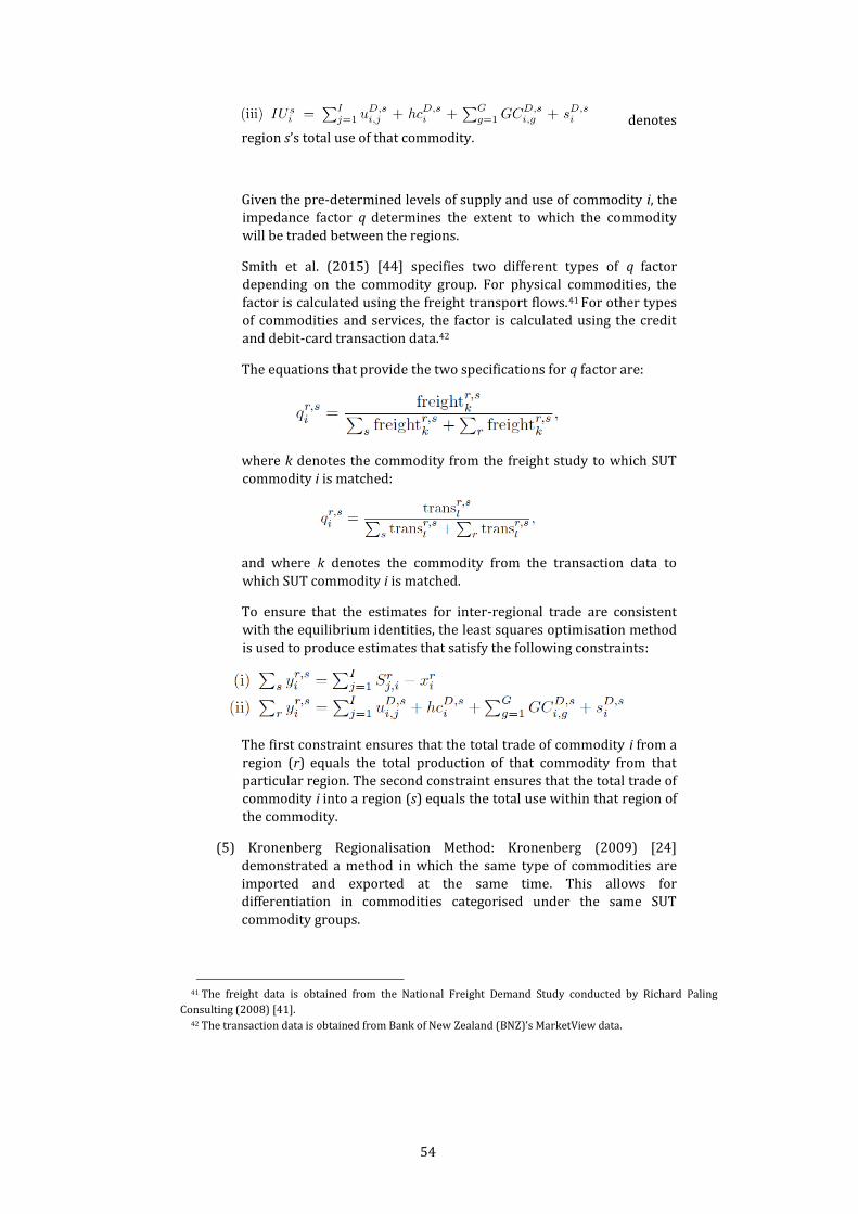
54
denotes region s’s total use of that commodity.
Given the pre-determined levels of supply and use of commodity i, the impedance factor q determines the extent to which the commodity
will be traded between the regions.
Smith et al. (2015) [44] specifies two different types of q factor
depending on the commodity group. For physical commodities, the
factor is calculated using the freight transport flows.41 For other types of commodities and services, the factor is calculated using the credit
and debit-card transaction data.42
The equations that provide the two specifications for q factor are:
where k denotes the commodity from the freight study to which SUT
commodity i is matched:
and where k denotes the commodity from the transaction data to
which SUT commodity i is matched.
To ensure that the estimates for inter-regional trade are consistent
with the equilibrium identities, the least squares optimisation method
is used to produce estimates that satisfy the following constraints:
The first constraint ensures that the total trade of commodity i from a
region (r) equals the total production of that commodity from that
particular region. The second constraint ensures that the total trade of commodity i into a region (s) equals the total use within that region of
the commodity.
(5) Kronenberg Regionalisation Method: Kronenberg (2009) [24]
demonstrated a method in which the same type of commodities are
imported and exported at the same time. This allows for differentiation in commodities categorised under the same SUT
commodity groups.
41 The freight data is obtained from the National Freight Demand Study conducted by Richard Paling
Consulting (2008) [41]. 42 The transaction data is obtained from Bank of New Zealand (BNZ)’s MarketView data.

55
The method is applied to the remaining set of commodities, which
mainly comprise services, using the process outlined in Smith et al.
(2015)[44] and Kronenberg (2009) [24].
For the application of the model, a coefficient called HETi is defined to denote the level of heterogeneity among all commodities grouped
under one category. This coefficient is estimated as:
The term xi +IMi is the balance of export and import of commodity i,
and γ and γ’ are the national use and production of i as defined in section 3.3.1 of this report. The heterogeneity coefficient is therefore
estimated by the extent that the commodity is traded across
international markets relative to its total domestic supply and use. All
import, export and supply data are available from the NSUT.
The level of cross-hauling or simultaneous import and export of a
commodity is denoted as , and estimated as:
where the terms ISir and IUir are as defined earlier. Therefore, the level
of cross-hauling is the total sum of domestic supply and use of a given
commodity in a region, scaled by how much products under the same
commodity category differ. This specification allows to increase in proportion to the increase in both the supply and use of the
commodity, but a less-than-proportional increase if only one of them
increases. Also, the more the products differ, the higher the cross-
hauling between regions.
The total inter-regional import and export of a given commodity i and
region r are then estimated as:
,
where (ISir−IUir) denotes the net surplus in production of commodity i
within r, and TVir denotes the total value of inter-regional trade in
commodity i for r, calculated as:
Finally, the estimate of inter-regional trade of commodity i for all
possible destination regions is calculated using the trade share
coefficient TRr,s as:
where
56
s ≠ r
The trade share coefficients are estimated using the MarketView data
on total sales by agents within region r to agents within region s, denoted as salesr,s.
Balancing the RSUT
As mentioned earlier, the estimates derived in the above steps can be further refined to ensure that the RSUT meets the market-clearing conditions.
In particular, the total supply of commodity i in region r has to equal the total use
of that commodity in that region:
Using the estimates from the above steps, (the
over-line indicates that they are estimates), the final estimates can be obtained by using the balance equation.
Using the estimates, the total supply of commodity i in region r, Sir and total use,
Uir can be estimated as:
The final use of commodity i in region r by industry j is then estimated by using
the least squares optimisation method:43
When the market-clearing condition is held, and .
The constrained optimisation equation is specified to reduce the squared
deviation of the estimate from the final target subject to the above market-clearing constraint.
Constructing the RSAM
For a given region (r), a RSAM is essentially of the same structure as the NSAM.44 The additional agent, the rest of New Zealand (RoNZ), represents the
transactions with the other regions in New Zealand. A number of components
43 Alternatively, a RAS (bi-proportional fitting method) can be used to estimate the final use of
commodities. Although both methods (optimisation and RAS) have a chance of producing an illogical solution, the RAS method is more prone to producing an out-of-equilibrium or an illogical solution.
44 As a consequence, the RSAM includes arbitrary regional measures, such as regional factor payments to ROW. Any regional measures not necessary for the EIA analysis on freshwater quality have been summed and modelled as a national-level measure in the sub-regional CGE model (including the freshwater-quality module).
57
derived for RSUT are used directly in RSAM. These components include Ur, hcr,
GCr, sr, IMr, xr, Sr, TY r and xr,s.
Other components (such as factors of production and transfer terms) are
derived using the appropriate regional proportions obtained from various data sources.
In this section, we explain the derivation of components not directly obtained
from the RSUT.
1. Labour Income Accounts: The total factor payments for labour input in
region r can be allocated to the households within the region, the RoNZ and the ROW.
The first step in deriving the value of labour income from the RoNZ
denoted as CoErronz is to estimate the value of total labour factor income for
RoNZ (CoERoNZ).
This can be calculated as the difference between the total national labour factor income, CoE (obtained from the NSUT) and the region r’s labour
factor income (CoEr from the RSUT).
That is, CoERoNZ = CoE − CoEr. The following steps demonstrate the
derivation of the labour factor income from r to ROW ( ), from
RoNZ to ROW ( ), from RoNZ to , and then finally from r
to RoNZ ( ).
: The labour factor income from region r to ROW is calculated using the regional GDP share of the total national labour
income payment to ROW. Implicit, in this estimation is the
assumption that the larger the GDP of the region, the larger the factor
payments made to ROW. The equation that demonstrates the
calculation is:
: The labour factor income from RoNZ to ROW is estimated
by taking the difference between the total labour factor payment to
ROW and the region r’s share of that payment. Once the region r’s payment to ROW is subtracted, the rest of the payments are made by
RoNZ. The equation that demonstrates this method is:
The value for CoErowr is as estimated in the previous step, while
CoERoW is from NSUT.
(iii) CoErronz: The total labour factor payment from RoNZ into r is
estimated by using the proportion of people who reside in r but
commute to RoNZ for work. This coefficient (cs,t) denotes the number

58
of people who live in region s but who commute to region t, and can
be calculated using the data from SNZ’s Census.45
The equation that demonstrates the estimation of is:
The bracketed term above indicates the total CoE payment from
RoNZ that remains within New Zealand.
: The total factor for income paid from domestic labour from enterprises in r to households in region r is estimated as:
The bracketed term indicates the total domestic regional share of
labour income, while the last term denotes the labour income paid from RoNZ to r.
: The labour factor payment from businesses in region r to
the households in RoNZ is estimated by the proportion of people who
live in RoNZ but who commute to r for work.
Again, the bracketed term indicates the total domestic regional share
of labour income, while the coefficient indicates the share of workers
who reside in RoNZ but work in region r.
2. Capital Return Accounts: Similar to the labour income accounts, the capital income for a given region r can be sourced from other regions within
New Zealand and the ROW.
The total capital factor payments to RoNZ are calculated as the difference between the total national payment and the capital payment in region r. That is, GOSronz = GOS − GOSr.
The regional transfer of GOS from RoNZ to . This transfer includes the region r’s share of enterprises located in RoNZ.
Typically, the GOSH comprises the imputed rent from the owner-occupied
dwellings and the return from capital investment into enterprises. To
separate the return on capital from the enterprises, the income from the
owner-occupied dwellings is estimated by the following coefficient dr as:
,
where, indicates the gross operating surplus from owner-occupied
dwellings in region r and denotes the consumption of fixed capital
45 SNZ Census, Usual Residential Areas and Workplace Areas by Main Means of Travel to Work. [47].
59
in owner-occupied dwellings in r. The denominator is the sum of the
national total for the two values.
Both values are derived from the RGDP and the SUTs. The national total
values are also available from the NAs. We also define the enterprise ownership coefficient, ϵ.
,
where, EC is the full-time equivalent employee count for each enterprise, and GU is a geographical business unit as defined by SNZ’s Geographic Unit
and Employee Data. The gross domestic product for each region r is
denoted as GDP and k denotes the New Zealand enterprise ownership
share information (in percentage units) as contained in SNZ’s Enterprises
and Full-Time Equivalent Persons Engaged by Degree of Overseas Equity and ANZSIC.
The region r’s share of gross operating surplus from enterprises in RoNZ
( ) is then estimated as:
,
where, GOSronz is as calculated above, and GOSGronz is the RoNZ share of the
government’s gross operating surplus calculated as GOSG−GOSGr. The
region r’s share of enterprises in RoNZ is estimated by .
(i) GOSEr: The gross operating surplus to enterprises in region r is
calculated as the sum of total surplus payments from RoNZ and the
regional total surplus after deducting the surplus payment to
households, government and RoNZ:
,
where, is calculated as below.
: The surplus payment from r to RoNZ is calculated as:
(iii) GOSHr: The regional share of surplus payment to households can be estimated as a proportion of the national surplus payment. That is,
GOSHr = drGOSH, where GOSH is directly obtained from the NSUT.46
(iv) GOSGr: The regional value of the government’s share of GOS is
calculated by summing the capital income of both central and local
government in each region.
,
46 This estimation can be refined by using the data on residents who usually live in each region, as demonstrated
in Smith et al. (2015)[44].
60
where, OSGir denotes the government industry i’s (Gi) gross operating
surplus in region r and CoFCGir denotes the government industry i’s
(Gi) consumption of fixed capital in region r.
3. Enterprise Account: The household transfers to enterprises for region r is
calculated using a coefficient that is used to estimate the given region’s
share of the national enterprise investment and another scalar that indicates RoNZ’s share. The total superannuation and pension fund
investment services provided by region r to s can be denoted as Rr,s. Then
indicates the total investment services provided from region r to
all of New Zealand and indicates the total services provided by r to the RoNZ.
Then the transfers from households in region r to enterprises in region r are calculated as:
The first term and the bracketed term together indicate the regional share
of the total household transfers to enterprise, while the last term indicates
the region r’s share of that transfer.
: The household transfer to enterprises from the households in RoNZ to enterprises in r. The equation that illustrates the estimation
is:
Then the total national household transfer to enterprises in region r
is the sum of the and :
(ii) rower: The transfer from the ROW to enterprises in region r is estimated using the regional GDP share:
(iii) ehr: The total enterprise transfer to household in region r is
estimated using the total share of investment held by households in
region r, denoted by Ir. The household investment I includes:
(1) entrepreneurial income from self-employment or casual and hobby income; (2) property income received from dividends; and
(3) property income received from other investments. Including
income from any portfolio investment entries. All data are available
from SNZ’s Household Economic Survey.
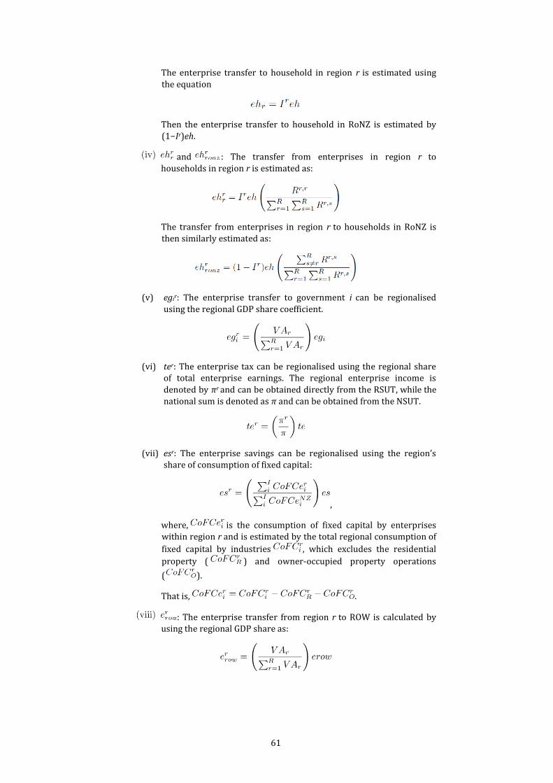
61
The enterprise transfer to household in region r is estimated using
the equation
Then the enterprise transfer to household in RoNZ is estimated by
(1−Ir)eh.
and : The transfer from enterprises in region r to
households in region r is estimated as:
The transfer from enterprises in region r to households in RoNZ is
then similarly estimated as:
(v) egir: The enterprise transfer to government i can be regionalised
using the regional GDP share coefficient.
(vi) ter: The enterprise tax can be regionalised using the regional share of total enterprise earnings. The regional enterprise income is
denoted by πr and can be obtained directly from the RSUT, while the
national sum is denoted as π and can be obtained from the NSUT.
(vii) esr: The enterprise savings can be regionalised using the region’s share of consumption of fixed capital:
,
where, is the consumption of fixed capital by enterprises within region r and is estimated by the total regional consumption of
fixed capital by industries , which excludes the residential
property ( ) and owner-occupied property operations
( ).
That is, .
: The enterprise transfer from region r to ROW is calculated by using the regional GDP share as:
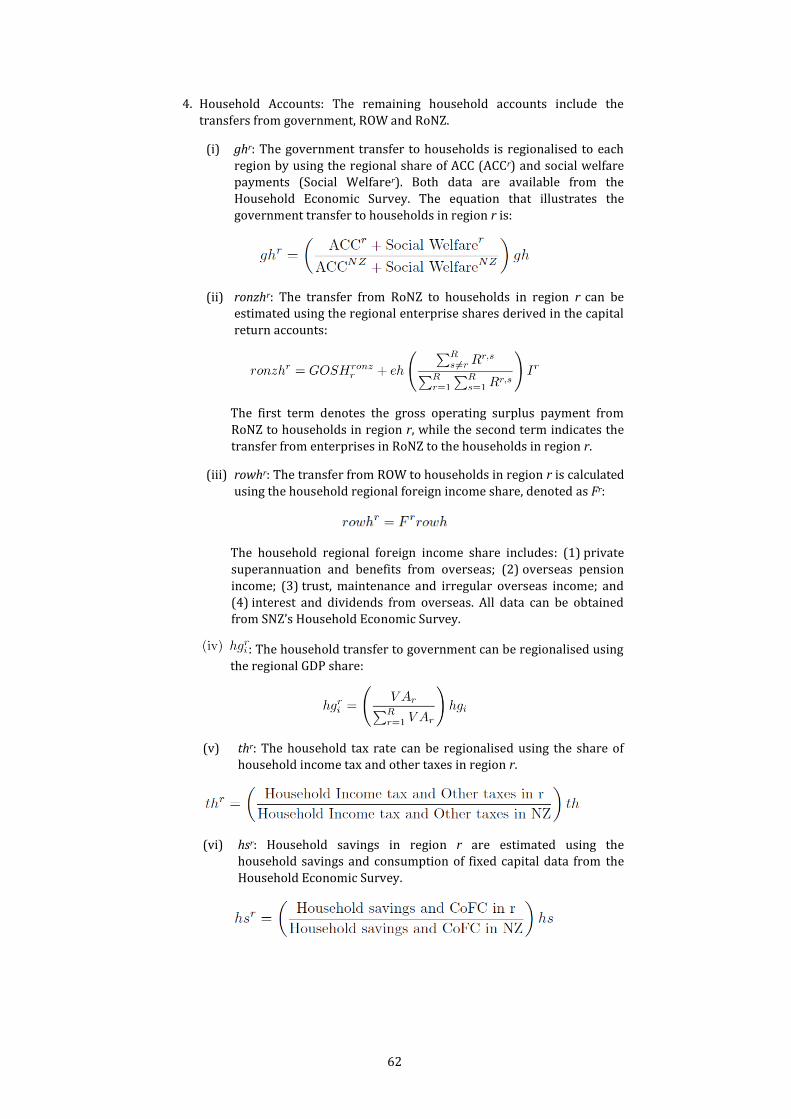
62
4. Household Accounts: The remaining household accounts include the
transfers from government, ROW and RoNZ.
(i) ghr: The government transfer to households is regionalised to each
region by using the regional share of ACC (ACCr) and social welfare payments (Social Welfarer). Both data are available from the
Household Economic Survey. The equation that illustrates the
government transfer to households in region r is:
(ii) ronzhr: The transfer from RoNZ to households in region r can be estimated using the regional enterprise shares derived in the capital
return accounts:
The first term denotes the gross operating surplus payment from
RoNZ to households in region r, while the second term indicates the
transfer from enterprises in RoNZ to the households in region r.
(iii) rowhr: The transfer from ROW to households in region r is calculated
using the household regional foreign income share, denoted as Fr:
The household regional foreign income share includes: (1) private
superannuation and benefits from overseas; (2) overseas pension
income; (3) trust, maintenance and irregular overseas income; and
(4) interest and dividends from overseas. All data can be obtained from SNZ’s Household Economic Survey.
: The household transfer to government can be regionalised using
the regional GDP share:
(v) thr: The household tax rate can be regionalised using the share of household income tax and other taxes in region r.
(vi) hsr: Household savings in region r are estimated using the household savings and consumption of fixed capital data from the
Household Economic Survey.
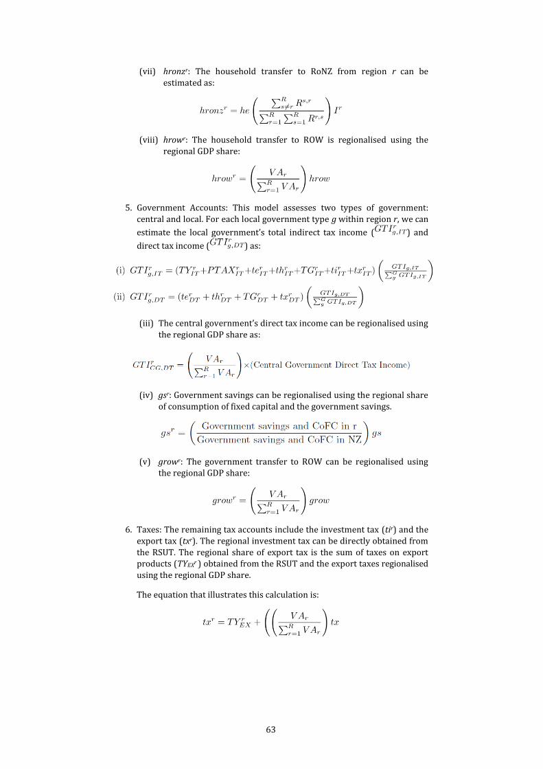
63
(vii) hronzr: The household transfer to RoNZ from region r can be
estimated as:
(viii) hrowr: The household transfer to ROW is regionalised using the
regional GDP share:
5. Government Accounts: This model assesses two types of government:
central and local. For each local government type g within region r, we can
estimate the local government’s total indirect tax income ( ) and
direct tax income ( ) as:
(iii) The central government’s direct tax income can be regionalised using
the regional GDP share as:
(iv) gsr: Government savings can be regionalised using the regional share
of consumption of fixed capital and the government savings.
(v) growr: The government transfer to ROW can be regionalised using the regional GDP share:
6. Taxes: The remaining tax accounts include the investment tax (tir) and the
export tax (txr). The regional investment tax can be directly obtained from
the RSUT. The regional share of export tax is the sum of taxes on export products (TYEXr ) obtained from the RSUT and the export taxes regionalised
using the regional GDP share.
The equation that illustrates this calculation is:

64
7. Savings Accounts: The only remaining RoNZ account is the savings by
RoNZ (ronzsr). This can be estimated as the balance of all other transfers
between region r and ronz. This estimation assumes that all remaining
transfers between region r and RoNZ are transfers of capital.
The savings from ROW (rowsr) is regionalised using the regional GDP
share.
The RSAM can be built using the regionalised elements estimated above. An
example of RSAM for a given region (r) is provided in Figure 5.
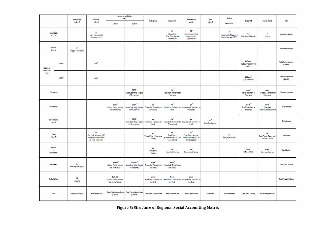
Figure 5: Structure of Regional Social Accounting Matrix

3.3.3 The sub-regional Social Accounting Matrix
The structure of the sub-regional SAM depends on the choice of a sub-regional
CGE method outlined in section 2.3. The main difficulty building the sub-regional
SAM is the availability of sub-regional data. At the time of writing this report, detailed methods of building the sub-regional SAM are not available. Yet the
method chosen is likely to be similar to the RSAM construction method.
Listed below is a possible strategy for building the sub-regional SAM.
• As noted in the spatial economic data section, the most detailed sub-
regional data available are SNZ BF and Census. The BF data includes employment by meshblock-level spatial locations and can be used to
estimate the industrial production levels of sub-regions and the
intermediate consumption associated with those production activities. The
Census data includes detailed household information and can be used to
estimate household demands for commodities within sub-regions. Together, this helps us to build the sub-regional supply-use tables.
• The broad structure of the sub-regional SAM will be similar to the RSAM,
but may include minor, secondary financial flows between agents. Their
status is because they may be hard to estimate. For example, all sub-
regions within the region (i.e., Auckland Council) have only one local
government. Sub-regionalising the local government is unrealistic in this example. Overall, the build method is likely to follow a similar approach
used to build the RSAM.
• The sub-regional SAM must be consistent with the regional SAM. For
example, the summation of the dairy product outputs of the sub-regions
must equal the same output estimated in the RSAM. Once individual components of sub-regional SAMs for all sub-regions are built, each SAM
will be matched to the RSAM using a ‘least squares constrained’
optimisation method. Here, the constraint is such that the summation of
individual components of the sub-regional SAM is matched to the
corresponding components in the RSAM.
3.4 Data requirements for incorporating a freshwater module
Currently, Auckland Council is building the necessary data to meet the NPS-FM.
This process includes full water accounting for the Auckland region and water
catchment models capable of deriving emission levels from water pollutants.
Initial consultation with the council’s research team revealed that the current
water accounts and pollution data are not suitable for the proposed CGE model. However, the research team confirmed that it is possible to numerically calculate
the data to meet the requirements for the CGE model. Subsequently, further
collaboration within the council is required.
Below are some of the key issues and observations for each of the freshwater
modules, (production, consumption, and abatement).
• Production: Current Auckland Council water accounts and pollution
models produce output data at highly aggregated level for the pollution
67
production module. Specifically, the pollution data will be broadly
categorised based on activities (e.g., industrial, business) and may not be
detailed enough for production-based pollution output in the CGE model
(categorised by the ANZSIC06-based 106 industry classifications from the supply-use tables).
Consequently, tracing specific water pollutant quantities to a specific
industry classification is difficult. For example, disaggregating the
quantities of zinc wastes from an industrial activity to industrial
classifications (e.g., chemical manufacturing and basic metal manufacturing) used in the CGE model is very difficult. This difference in
how economic activities are categorised arises because the water accounts
and pollution model is based primarily on spatial land uses. In contrast,
the CGE model is based on monetary data, where it is difficult to categorise
the spatial land uses into specific industry classifications. This is because a parcel of land maybe used for multiple uses.47
• Consumption: As the outputs from Auckland Council water accounts and
pollution model are spatially explicit, water pollution from household
consumption for each sub-region may be derived by: (1) calculating the
average pollution per population from the residential areas within the sub-region; and then (2) multiplying that average pollution per population by
the total sub-region population.
• Abatement: Initial data mining revealed that the data required to build the
abatement curve is insufficient. Abatement data for the agricultural
industries maybe built using farm-level financial models such as FARMAX. Even so, such models are not available for either the manufacturing sector
or service sector, which together make up a large portion of Auckland’s
economy.
Consequently, simpler partial equilibrium financial models may be built
for each industry. For example, a firm chooses a level of abatement investment to maximise profit based on exogenous factors such as
subsidies. In turn, it can collect the data necessary to build abatement
curves by running multiple simulation runs of the partial-equilibrium
model and varying the exogenous factors.
47 For example, a multi-storey building in a business section can be used for retail on the ground
level and business services on the upper levels.
68
4 Summary and Conclusions
4.1 Summary of Stage 2
The CGE model framework introduced in this report is a multi-regional one.
The framework involves modelling the decisions and transactions of households, producers, and central and local government. Each agent in the model faces its
own optimisation problem subject to its budget constraints. Households make
choices to maximise their welfare subject to their budget constraints while
producers maximise their profits subject to their cost constraints. The model
outputs the demand and supply and prices of every traded commodity in a state
of general equilibrium. This is where all agents are doing the best they can and markets clear (i.e., demand for a commodity equals its supply).
We have incorporated water pollution emission and abatement sectors to into
production and consumption processes. The impact of different policy measures
(such as changes in tax rate and subsidies) can be examined at national, regional
and sub-regional levels.
One main feature (also a challenge) in building the comprehensive sub-regional
model is in modelling various sources of freshwater pollution and the effect of
policy measures on different regions within the model.
4.2 Summary of Stage 3
The sub-regional CGE model examines policy impacts at the national, regional
and sub-regional levels. This involves an extensive search for corresponding data at those levels. The detailed data requirements for each level are discussed
in section 3 of this report.
In summary, the basis for our national-level supply and use of resources is
provided by the 2013 NSUT (Input-Output) table published by SNZ.
Correspondingly, the state of the economy is based on the national accounts for the same year. We would use both sets of data to build the NSAM.
We would then regionalise NSAM by incorporating the regional data obtained
from RGDP and various other sources. The resulting RSUT and RSAM would
capture the transactions of agents for the 15 main regions within New Zealand.
We can then disaggregate the regional level data into the sub-regional level using the FMUs. This step is expected to incur the highest cost for data gathering, as
information at a sub-regional level is scarce and difficult to source.
4.3 Conclusions
The CEU at Auckland Council is proposing to develop a sub-regional CGE model
to assess how current policy and planning initiatives affect economy and land
use in Auckland. The key characteristic of the model is that it is multi-regional at
a sub-regional level. That is, the model is multi-regional CGE model with the Auckland region, spatially separated into CB level sub-regions. This allows for
feedback between sub-regions, as well as between other parts of New Zealand,
and shows the sub-regional distribution of the economic impacts. Importantly,

69
the model is able to assess the inter-regional distribution of the economic
impacts, winners and losers associated with exogenous shocks and policies.
The model provides a more realistic representation of Auckland’s
economy48than a regional CGE model or partial equilibrium approaches, and can be used to examine a diverse range of policies and EIAs. In addition, the model
structure and implementation (eg, by using computer codes) is generalised and
can be easily used for other spatial definitions (such as other regions in
New Zealand).
4.3.1 A summary of how the CGE model assesses freshwater quality
In this report, we identified the CGE model setup for assessing the economic
impacts associated with initiatives that set limits for freshwater quality.
We have specified a framework that incorporates: (i) a multi-regional, sub-regional spatial level; (ii) freshwater-quality management module that examines
the production and consumption of pollution; and (iii) an abatement technology
module that allows for detailed changes in production input requirements in
response to exogenous policy shocks.
The proposed CEU sub-regional CGE model incorporating freshwater-quality management is designed to model how water pollutions are generated by both
production and consumption activities within an economy. In addition, the
model incorporates an endogenous abatement module where producers within
the economy adjust their production and investment behaviours in response to
policy measures. The model can therefore be used to test and compare the effects various policies on freshwater quality for each FMU at the same time.
The model includes production and consumption (primary) flows as well as
accounting and financial (secondary) flows within the economy, and reproduces
the behaviour of agents within an economy. Further, the CGE model offers
interdependence between agents and regions, represents a complete picture of Auckland’s economy, and provides robust, economic impact outputs associated
with policies focused on the quality of fresh water.
We can use the model to infer how combinations of freshwater policies for each
FMU affect the economy of that FMU as well as the Auckland region and other
parts of New Zealand. It is important to note that the model can assess economic consequences of urban development, land-use planning and growth policies
about freshwater quality, as well as the reverse (i.e., how policy decisions about
freshwater quality affect the economy and land use). Similarly, the model can
include non-freshwater policies (e.g., greenhouse gas emissions) faced by the
council and show the effects on freshwater quality, as well as interaction effects between freshwater policies and non-freshwater policies.
This study also looked at the sources of data for building the CGE model and
identified potential data constraints. We found that, currently, insufficient data is
available to build the national and multi-regional CGE model framework.
However, the council is currently developing the pollution, abatement and water
48 For example, a sub-region mainly used as a residential area will show different pollution
emission levels and pollutant composition from a mainly industrial area. The approach taken by the sub-regional housing model should be able to match the economic and demographic composition to each sub-region.

70
account data required for sub-regional housing CGE model to study the impact of
pollutant emission and abatement technology. This is required to meet the NPS-
FM standards.
4.3.2 The benefits of using an expanded CGE model to assess the implications of both freshwater quality and other economic initiatives
The purpose of this study was to improve our understanding of the potential and
challenges if we expand the sub-regional CGE model to account for impacts of freshwater policies on economic growth and development. In addition, the CGE
model proposed in this study aims to help us understand the potential economic
consequences of policies under NPS-FM.
From this study and the literature review conducted in Stage 1 of the study, we
found numerous benefits of using the CGE model to assess the economic implications of both freshwater quality and other environmental policy
initiatives. Further, we found that a sub-regional CGE model at FMUs level is
required to conduct a robust economic impact analysis of proposed freshwater-
quality policies in Auckland. Eight key benefits for developing the model are
noted below.
1. CBA methods (mainly analysing primary sectors) and IO methods (without
behavioural change) used in EIAs of other regions in New Zealand do not
incorporate overall changes in production behaviours. In comparison, the
CGE model incorporates price dynamics, where an exogenous shock or a
policy change affects prices of commodities. This in turn affects the consumption and production behaviours of the agents within the economy.
A key objective of the study is to build a CGE modelling capacity within the
council so we can use the CGE model to conduct future EIAs within the
council.
2. Despite the wide use of CGE model in assessing economic implications of environmental policies (as evidenced in the international literature), in
New Zealand most EIAs of water policies are conducted using a mix of CBA
and IO approach. Our review of the international literature showed
numerous studies on the EIA of economic growth and water quality. These
studies on water quality were completed relatively recently, and we observed a growing interest in this issue.
3. Auckland has different economic structures from the rest of New Zealand.
Auckland’s economy is dominated by manufacturing and service
industries, while primary industries occupy a relatively small portion of
the economy. As manufacturing and services industries are more flexible in changing their production behaviours, any policy initiatives will have a
greater impact on these industries. In addition, Auckland has experienced
an unprecedented pressure on its infrastructure, such as freshwater
supply, as a result of the increase in net migration and general population
growth. The proposed CGE model will try to capture these features of the Auckland economy as realistically as possible.
4. Policy initiatives affect demand and the price of underlying factors of
production (e.g., labour, capital and land). CGE models can capture this fact.
For example, certain policies may lower demand for land from the
71
production side of the economy. In contrast, the key issue for Auckland is
urban intensification and housing, where the availability and the price of
land is an important consideration. The CGE model can incorporate both
the patterns of household demand for housing land and demand from the production sector for land. Subsequently, we can use the model to analyse
potential impacts of freshwater policy initiatives on housing land prices
and supply (as well as on other aspects of the economy).
5. CGE models are useful in analysing the impacts of multiple policy
initiatives at the same time. As CGE models search for an optimal economic decision for all agents (e.g., production, households, and governments) in
the economy, and include both supply and demand side of economic
activities by these agents, they are flexible in including different types of
exogenous and policy shocks. Instruments that set the limits for
freshwater quality affect the economy through various channels, and a CGE model captures this.
In addition, CGE models can incorporate seemingly unrelated exogenous
policy shocks. They can calculate the overall impacts of these policies on
the economy and any associated externalities. For example, the models
could include water quality and housing policy initiatives to determine the combined impacts on the economy and the environment.
6. The sub-regional CGE model includes inter-spatial relationships within
the region and the rest of New Zealand. Therefore, the model can assess
how a policy in a region or a sub-region can affect other regions and sub-
regions. For example, the effect of reduction in economic output of the Auckland region caused by a freshwater policy will flow on to other areas
within New Zealand. Further, the model can identify the sub-regional and
inter-regional winners and losers of implementing freshwater-quality
policies.
7. The CGE model can assess opportunity costs associated with those policies where a comparison between the economic impacts of different policies meeting the limits is possible. Typically, a CGE model includes a base case
economic scenario (i.e., business as usual). The base case is used as a benchmark and compared against outputs resulting from exogenous
shocks and policy scenarios. As such, the model can use changes in outputs against a benchmark for each scenario to compare different policies. Building a comprehensive sub-regional housing CGE model framework for
Auckland will not only enable the council to develop the capability to study the impact of various policy implications within Auckland. It will also
contribute to studying other regions in New Zealand.
72
References
[1] Auckland Council. The Proposed Auckland Unitary Plan. Auckland, Auckland
Council. 2013
[2] Bank of New Zealand. MarketView. Bank of New Zealand. 2013
[3] Berck, P., Robinson, S., and Goldman, G. The use of computable general
equilibrium models to assess water policies. (pp 489–509). Springer US. 1991
[4] Bhringer, C., and Lschel, A. Computable general equilibrium models for
sustainability impact assessment: Status quo and prospects. Ecological
Economics, 60(1), 49–64. 2006
[5] Brouwer, R., and Hofkes, M. Integrated hydro-economic modelling:
Approaches, key issues and future research directions. Ecological Economics,
66(1), 16–22. 2008
[6] Brouwer, R., Hofkes, M., and Linderhof, V. General equilibrium modelling of
the direct and indirect economic impacts of water quality improvements in
the Netherlands at national and river basin scale. Ecological Economics,
66(1), 127–140. 2008
[7] Conrad, K. Computable general equilibrium models in environmental and
resource economics. Discussion papers/Institut für Volkswirtschaftslehre
und Statistik; Department of Economics, Universitt Mannheim, 601. 2005
[8] Daigneault, A., McDonald, H., Elliott, S., Howard-Williams, C., Greenhalgh, S.,
Guysev, M., Kerr, S., Lennox, J., Lilburne, L., Morgenstern, U. and Norton, N.
Evaluation of the impact of different policy options for managing to water
quality limits. Wellington, Ministry for Primary Industries 2012
[9] Daigneault, A., Samarasinghe, O., and Lilburne, L. Modelling economic
impacts of nutrient allocation policies in Canterbury Hinds Catchment: final
report. Landcare Research. 2013
[10] Dellink, R., Hofkes, M., van Ierland, E., and Verbruggen, H. Dynamic
modelling of pollution abatement in a CGE framework. Economic Modelling,
21(6), 965–989. 2004
[11] Dellink, R., and Van Ierland, E. Pollution abatement in the Netherlands: a
dynamic applied general equilibrium assessment. Journal of Policy Modeling,
28(2), 207–221. 2006
[12] Deng, X., Zhao, Y., Wu, F., Lin, Y., Lu, Q., and Dai, J. Analysis of the trade-off
between economic growth and the reduction of nitrogen and phosphorus
emissions in the Poyang Lake Watershed, China. Ecological Modelling,
222(2), 330–336. 2011
[13] Diukanova, O., Andrew, R., and Lennox, J. Emission Trading in New Zealand:
Computable General Equilibrium Model and Evaluation: Landcare Research.
Landcare Research. 2008
[14] Ejaz Qureshi, M., Proctor, W., Young, M. D., and Wittwer, G. The economic
impact of increased water demand in Australia: A computable general
73
equilibrium analysis. Economic Papers: A journal of applied economics and
policy, 31(1), 87–102. 2012
[15] Glaeser, E. L. Agglomeration economics. Economic Papers: A journal of
applied economics and policy, 31(1), 87–102. (Ed.). (2010).University of Chicago Press. 2010
[16] Grimes, A. Infrastructure and regional economic growth. Handbook of
Regional Science (pp 331–352). Springer Berlin Heidelberg. 2014
[17] Grimes, A. and Liang, Y. Spatial determinants of land prices: Does
Auckland’s metropolitan urban limit have an effect? Applied Spatial Analysis
and Policy, 2(1), 23–45. 2009
[18] Hansjrgens, B. Economic valuation through cost-benefit analysis,
possibilities and limitations. Toxicology, 205(3), 241–252. 2004
[19] Infometrics General equilibrium analysis of options for meeting
New Zealand’s international emissions obligations: Report prepared for
Emissions Trading Group. Infometrics, Wellington. 2008
[20] Jiang, L., Wu, F., Liu, Y., and Deng, X. Modeling the impacts of urbanization
and industrial transformation on water resources in China: an integrated
hydro-economic CGE analysis. Sustainability, 6(11), 7586–7600. 2014
[21] Johansen, L. A multisectoral Model of Economic Growth. North-Holland 2nd edition, Amsterdam. 1960
[22] Kaye-Blake, B., Schilling, C., Monaghan, R., Vibant, R., Dennis, S., and Post, E.
Potential impacts of water-related policies in Southland on the agricultural
economy and nutrient discharges. NZIER report to the Ministry for the
Environment. 2013
[23] Kim, J. H. Effects of Emissions on Trading Scheme on the New Zealand
Economy. A thesis submitted to the University of Auckland in fulfilment of
the requirements for the degree of Master of Commerce. 2013
[24] Kronenberg, T. Construction of regional input-output tables using
nonsurvey methods: the role of cross-hauling. International Regional
Science Review, 32(1): 4064. 2009
[25] Leontief, W., and Strout A. Multi-regional Input-Output Analysis. Structural Interdependence and Economic Development. New York: St. Martin’s Press.
1963
[26] Lennox, J. A., and Van Nieuwkoop, R. Output based allocations and revenue
recycling: Implications for the New Zealand Emissions Trading Scheme.
Energy Policy, 38(12), 7861–7872 2010
[27] Linneman, H. An Econometric Model of International trade flows. Amsterdam:
North Holland Publishing Co. 1966
[28] Luckmann, J., and McDonald, S. STAGE W: an applied general equilibrium
model with multiple types of water, technical documentation. 2014

74
[29] Market Economics Ltd. Southland Region Economic profile and significant
water issues. Report to the Ministry for the Environment. 2013
[30] Market Economics Ltd. Economic Impacts of Rotorua Nitrogen Reduction.
Report to the Bay of Plenty Regional Council. 2015
[31] McDonald, G. Integrating economics and ecology: a systems approach to
sustainability in the Auckland region. A thesis presented to Massey
University in partial fulfilment of the requirements for the degree of Doctor
of Philosophy, Palmerston North. 2005
[32] Ministry of Business, Innovation and Employment. Monthly Regional Tourism Statistics. Wellington: Ministry of Business, Innovation and
Employment. 2016
[33] Ministry for the Environment. Resource Management Act 1991 (RMA).
Wellington: Ministry for the Environment. 2010
[34] Ministry for the Environment. A guide to section 32 of the Resource
Management Act: Incorporating changes as a result of the Resource
Management Amendment Act 2013. Wellington: Ministry for the
Environment. 2014
[35] Nimmo-Bell & Company Ltd. Economic effects of Horizons One Plan Change.
Report to the Horizons Regional Council and Dairy NZ. 2013
[36] NIWA. Waikato River Independent Scoping Study. Report to the Ministry for the Environment. 2010
[37] NZIER. The Impact of the Proposed Emissions Trading Scheme on
New Zealand’s Economy. Wellington. 2008
[38] NZIER and Infometrics. Economic modelling of New Zealand climate change
policy: Report to the Ministry for the Environment. Wellington. 2009
[39] NZIER and Infometrics. Macroeconomic impacts of the New Zealand
Emissions Trading Scheme: A Computable General Equilibrium analysis: Final
Report to the Ministry for the Environment. Wellington. 2011
[40] Parker, C. Housing supply, choice and affordability. Auckland: Auckland
Council. 2015
[41] Richard Paling Consulting. National Freight Demand Study 2008. Report
prepared for the Ministry of Transport, NZ Transport Agency and the
Ministry of Economic Development. 2008
[42] Robson, N. A multi-regional computable general equilibrium model for New Zealand. A thesis submitted to the Victoria University of Wellington in fulfilment of the requirements for the degree of Doctor of Philosophy, Wellington. 2012
[43] Scrieciu, S. S. The inherent dangers of using computable general equilibrium
models as a single integrated modelling framework for sustainability
impact assessment. A critical note on Bhringer and Lschel (2006),
Ecological Economics, 60(4), 678–684. 2007

75
[44] Smith, N. J, Zhang, Y, Cardwell, R, McDonald, G. W, Kim, J. H, and Murray, C. F.
Development of a Regional Social Accounting Framework for New Zealand.
Market Economics Ltd. 2015
[45] Stevens, A. The application and limitations of cost-benefit assessment (CBA)
for intelligent transport systems. Research in Transportation Economics, 8,
91–111. 2004
[46] Statistics New Zealand. Information about the National Accounts: Glossary
Terms. Wellington: Statistics New Zealand. 2006
[47] Statistics New Zealand. 2013 Census Wellington: Statistics New Zealand.
2013
[48] Statistics New Zealand. 2013 National Supply-Use Table. Wellington: Statistics New Zealand. 2016
[49] Statistics New Zealand. 2015 Tourism Satellite Account. Wellington:
Statistics New Zealand. 2016
[50] Statistics New Zealand. 2015 House Economic Survey. Wellington: Statistics
New Zealand. 2016
[51] Statistics New Zealand. 2013 New Zealand Business Frame. Wellington:
Statistics New Zealand. 2013
[52] Statistics New Zealand. 2013 Harmonised System for Trade. Wellington:
Statistics New Zealand. 2013
[53] Statistics New Zealand. 2013 Institutional Sector Accounts. Wellington: Statistics New Zealand. 2016
[54] Statistics New Zealand. 2015 Regional Gross Domestic Product. Wellington:
Statistics New Zealand. 2016
[55] Statistics New Zealand. National Accounts: Year ended March 2015.
Wellington: Statistics New Zealand. 2016
[56] Torshizian, E. Are We Limiting Regional Development by Requiring Planning
Permissions? North American Regional Science Conference. 2015
[57] Torshizian, E. A Positive Expected Future Rent or A Negative Supply Effect? A
Study of Auckland’s MUL Expansion. mimeo. 2016
[58] Torshizian, E., and Chitale, H. Affordability Decompositions for Auckland.
mimeo. 2016
[59] United Nations. Handbook of Input-Output Table Compilation and Analysis.
And Handbook of National Accounting: Studies in Methods. New York: United
Nations. 1999
[60] Watson, P. S., and Davies, S. Modeling the effects of population growth on
water resources: a CGE analysis of the South Platte River Basin in Colorado.
The Annals of Regional Science, 46(2), 331–348. 2011

76
[61] Xie, J., and Saltzman, S. Environmental policy analysis: an environmental
computable general-equilibrium approach for developing countries. Journal
of Policy Modeling, 22(4), 453–489. 2000
[62] Yeoman, R., Kim, J. H, McDonald, G., and Zhang, Y. Modelling regional general
equilibrium for the Auckland Region. NZCEE Research Monograph. 2009
[63] Zhang, Y, McDonald, G. W, Nixon, P, and Smith, N. J. Development of a Regional Social Accounting Framework for New Zealand. NZCEE Research Monograph
Series—No.15. 2008
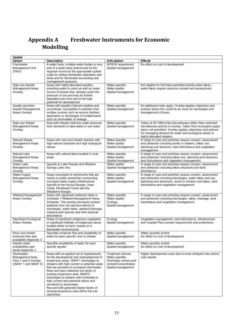
77
Appendix A Freshwater Instruments for Economic
Modelling

78

79

80
Appendix B Data Sources for NSAM
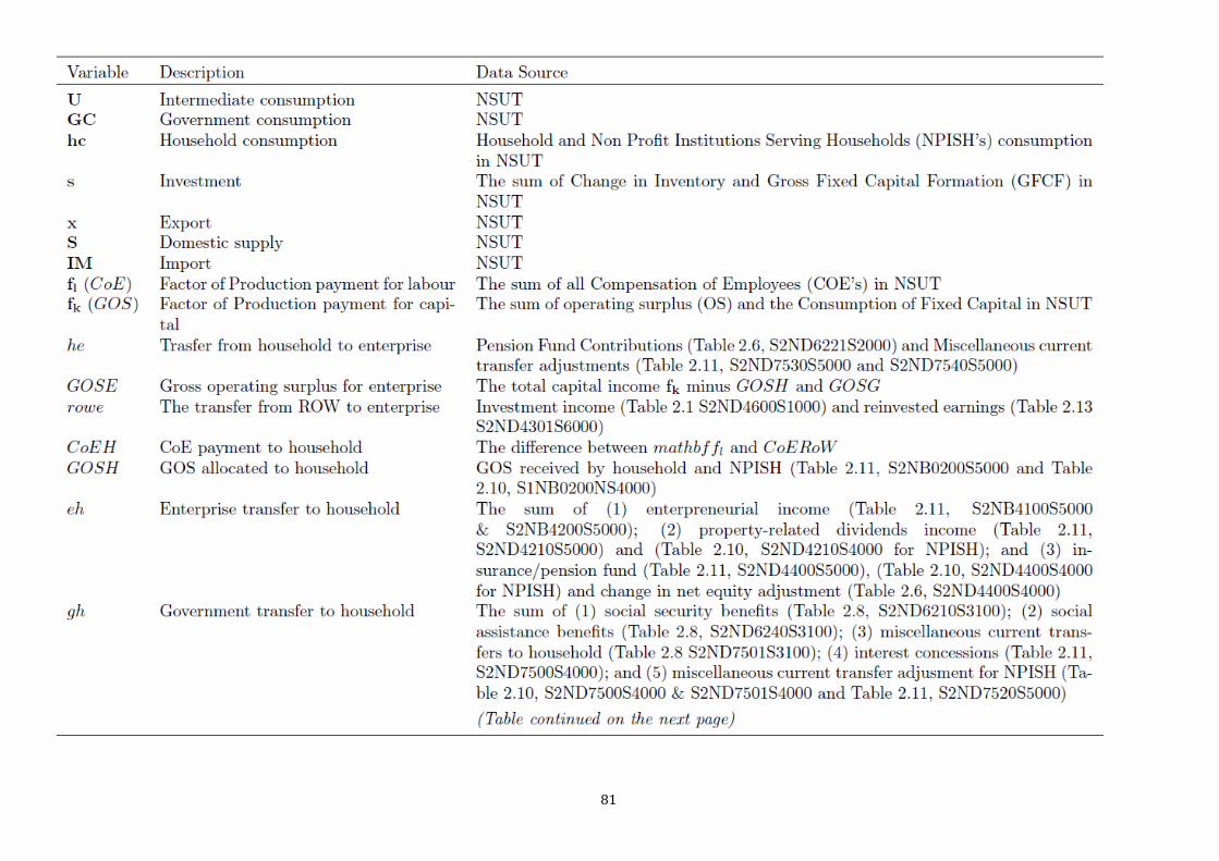
81
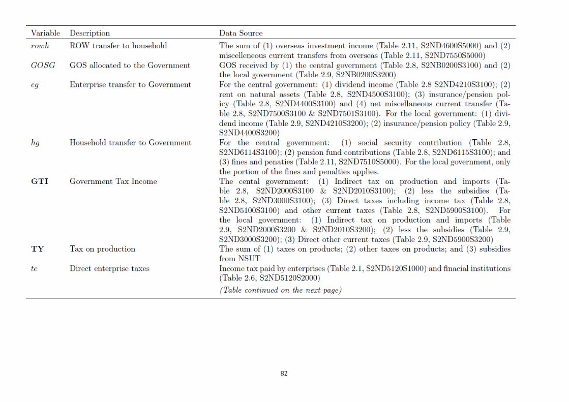
82
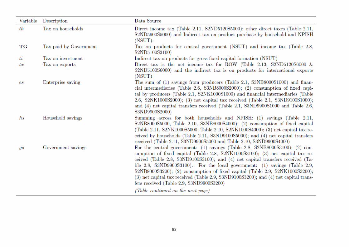
83

84