Ab

Ta

b

a

ARRAA

KNDM

1

irpsaWpda(Ict

r

(

h0

Precision Engineering 39 (2015) 47–55

Contents lists available at ScienceDirect

Precision Engineering

jo ur nal ho me p age: www.elsev ier .com/ locate /prec is ion

comparison study of algorithms for surface normal determinationased on point cloud data

ao Songa,∗, Fengfeng(Jeff) Xib, Shuai Guoa, Zhifa Minga, Yu Linb

Shanghai Key Laboratory of Intelligent Manufacturing and Robotics, HC206A, Shanghai University, 99 Shangda Road, BaoShan District, Shanghai, ChinaDepartment of Aerospace Engineering, Ryerson University, 350 Victoria Street, Toronto, ON M5B 2K3, Canada

r t i c l e i n f o

rticle history:eceived 5 February 2014eceived in revised form 29 April 2014ccepted 3 July 2014vailable online 21 July 2014

eywords:ormal determinationynamic sampling methodeasuring error

a b s t r a c t

Robot applications in manufacturing of aircraft sheet metal parts require real-time methods for deter-mining the surface normal using a digitized point data set measured by a 3D laser scanner. For this reason,six archived surface normal algorithms are compared. Though using different weights, these methods areall set to determine the surface normal at a given point by averaging the surface normals of the adjacentfacets. In this paper, a comparison study is designed with a nearest neighboring method searching foradjacent facets, along with the introduction of a dynamic sampling method to investigate the effect ofthe resolution of a data set on the accuracy of surface normal determination. Three performance indicesare proposed including the total number of final data points, the number of times of up-sampling andthe total computing time. Three geometric models are considered including a sphere representing an air-

craft cockpit, a cylinder representing a fuselage, and an ellipsoid representing a wing. The laser scannererror is modeled by a log-normal distribution. While all the six methods can generate satisfactory resultsin error-free case, the simulation results indicate that in error case MWE (mean weighted equally) andMWAAT (mean weighted by areas of adjacent triangles) are not favorable while the other four methodsexhibit no obvious difference.

© 2014 Elsevier Inc. All rights reserved.

. Introduction

In recent years, more and more robotics technology is beingntroduced to automate aircraft manufacturing processes, such asobotic drilling, robotic riveting, and robotic mirror milling. Therecision of these robotic operations is largely dependent on theurface normal of a sheet metal part that in turn defines the toolpproach direction for the drill or the rivet gun or the milling cutter.hile aircraft sheet metal parts, such as fuselage panels and wing

anels, are made according to CAD models, the actual shapes willeviate due to manufacturing tolerances. One way to obtain thectual surface normal would be to utilize the three-dimensional3D) laser scanning technology developed for surface digitization.ts applications spans from 3D urban modeling, industry survey,ulture relic preservation, 3D role modeling, reverse engineering

o surface measurement [1].

Over the last decade, research has been carried out on surfaceeconstruction using point cloud data. Alexa [2], Dey [3] and Kolluri

∗ Corresponding author. Tel.: +86 13764395023.E-mail addresses: songtao43467226@shu.edu.cn, songtao43467226@163.com

T. Song).

ttp://dx.doi.org/10.1016/j.precisioneng.2014.07.005141-6359/© 2014 Elsevier Inc. All rights reserved.

[4] developed the respective methods for surface reconstructionthrough surface normal. OuYang and Feng [5] found that the reli-able surface normal determination based on 3D laser scanningdata set was essential to CAD model construction. Zheng [6] pro-posed a method for object recognition from scanning point cloudbased on surface normal and curvature. Calderon [7] put forward analgorithm for surface normal determination using a neighborhoodstrategy based on local piecewise planes, and this algorithm greatlyimproved the accuracy of surface normal determination. Gong [8]proposed a novel method to measure the surface normal of an air-craft skin in order to improve the precision and efficiency of holedrilling. For aircraft panel mirror milling, Zhang [9] found that sur-face normal was critical to ensuring that the cutting tool path beconsistent with the skin surface being machined.

In general, the surface normal of a digitized surface cannot bemeasured directly, and it must be determined based on point clouddata either by generating a polygon model or by fitting a paramet-ric surface. Archived surface normal determination methods can bedivided into two categories: averaging method and optimization-

based method [10], with the former being more efficient than thelatter. The averaging method uses a polygon model to approximatea surface and determines the surface normal at a given point asa weighted sum of the surface normals of the facets surrounding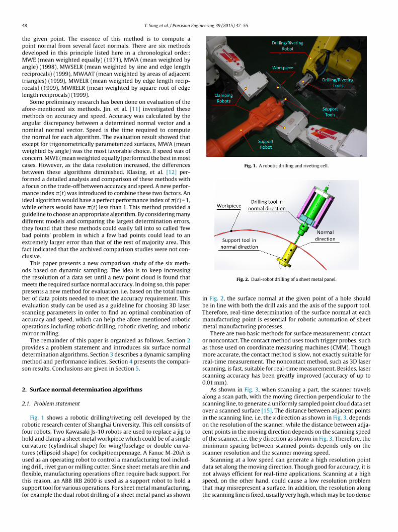

4 Engineering 39 (2015) 47–55

tpdMartrl

amantewccbfamiwgdtbefc

otmpbesaom

pdms

2

2

rfhctuifltsf

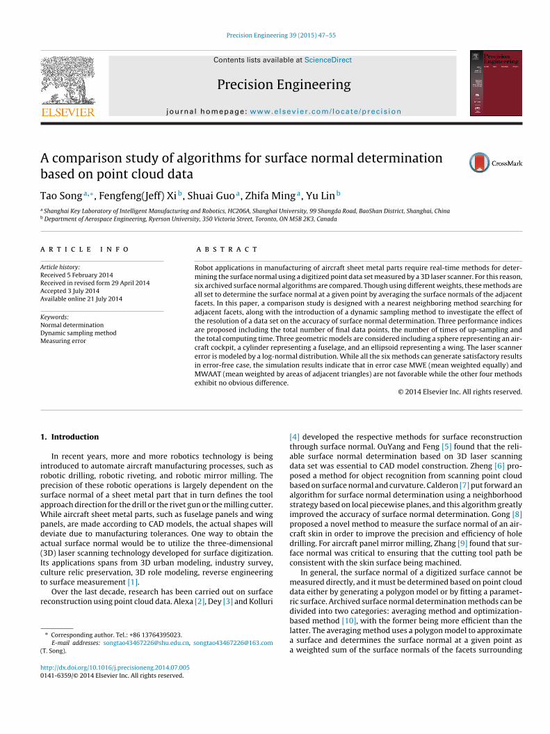
Fig. 1. A robotic drilling and riveting cell.

8 T. Song et al. / Precision

he given point. The essence of this method is to compute aoint normal from several facet normals. There are six methodseveloped in this principle listed here in a chronological order:WE (mean weighted equally) (1971), MWA (mean weighted by

ngle) (1998), MWSELR (mean weighted by sine and edge lengtheciprocals) (1999), MWAAT (mean weighted by areas of adjacentriangles) (1999), MWELR (mean weighted by edge length recip-ocals) (1999), MWRELR (mean weighted by square root of edgeength reciprocals) (1999).

Some preliminary research has been done on evaluation of thefore-mentioned six methods. Jin, et al. [11] investigated theseethods on accuracy and speed. Accuracy was calculated by the

ngular discrepancy between a determined normal vector and aominal normal vector. Speed is the time required to computehe normal for each algorithm. The evaluation result showed thatxcept for trigonometrically parameterized surfaces, MWA (meaneighted by angle) was the most favorable choice. If speed was of

oncern, MWE (mean weighted equally) performed the best in mostases. However, as the data resolution increased, the differencesetween these algorithms diminished. Klasing, et al. [12] per-ormed a detailed analysis and comparison of these methods with

focus on the trade-off between accuracy and speed. A new perfor-ance index �(t) was introduced to combine these two factors. An

deal algorithm would have a perfect performance index of �(t) = 1,hile others would have �(t) less than 1. This method provided a

uideline to choose an appropriate algorithm. By considering manyifferent models and comparing the largest determination errors,hey found that these methods could easily fall into so called ‘fewad points’ problem in which a few bad points could lead to anxtremely larger error than that of the rest of majority area. Thisact indicated that the archived comparison studies were not con-lusive.

This paper presents a new comparison study of the six meth-ds based on dynamic sampling. The idea is to keep increasinghe resolution of a data set until a new point cloud is found that

eets the required surface normal accuracy. In doing so, this paperresents a new method for evaluation, i.e. based on the total num-er of data points needed to meet the accuracy requirement. Thisvaluation study can be used as a guideline for choosing 3D lasercanning parameters in order to find an optimal combination ofccuracy and speed, which can help the afore-mentioned roboticperations including robotic drilling, robotic riveting, and roboticirror milling.The remainder of this paper is organized as follows. Section 2

rovides a problem statement and introduces six surface normaletermination algorithms. Section 3 describes a dynamic samplingethod and performance indices. Section 4 presents the compari-

on results. Conclusions are given in Section 5.

. Surface normal determination algorithms

.1. Problem statement

Fig. 1 shows a robotic drilling/riveting cell developed by theobotic research center of Shanghai University. This cell consists ofour robots. Two Kawasaki Js-10 robots are used to replace a jig toold and clamp a sheet metal workpiece which could be of a singleurvature (cylindrical shape) for wing/fuselage or double curva-ures (ellipsoid shape) for cockpit/empennage. A Fanuc M-20iA issed as an operating robot to control a manufacturing tool includ-

ng drill, rivet gun or milling cutter. Since sheet metals are thin and

exible, manufacturing operations often require back support. Forhis reason, an ABB IRB 2600 is used as a support robot to hold aupport tool for various operations. For sheet metal manufacturing,or example the dual robot drilling of a sheet metal panel as shown

Fig. 2. Dual-robot drilling of a sheet metal panel.

in Fig. 2, the surface normal at the given point of a hole shouldbe in line with both the drill axis and the axis of the support tool.Therefore, real-time determination of the surface normal at eachmanufacturing point is essential for robotic automation of sheetmetal manufacturing processes.

There are two basic methods for surface measurement: contactor noncontact. The contact method uses touch trigger probes, suchas those used on coordinate measuring machines (CMM). Thoughmore accurate, the contact method is slow, not exactly suitable forreal-time measurement. The noncontact method, such as 3D laserscanning, is fast, suitable for real-time measurement. Besides, laserscanning accuracy has been greatly improved (accuracy of up to0.01 mm).

As shown in Fig. 3, when scanning a part, the scanner travelsalong a scan path, with the moving direction perpendicular to thescanning line, to generate a uniformly sampled point cloud data setover a scanned surface [15]. The distance between adjacent pointsin the scanning line, i.e. the x direction as shown in Fig. 3, dependson the resolution of the scanner, while the distance between adja-cent points in the moving direction depends on the scanning speedof the scanner, i.e. the y direction as shown in Fig. 3. Therefore, theminimum spacing between scanned points depends only on thescanner resolution and the scanner moving speed.

Scanning at a low speed can generate a high resolution pointdata set along the moving direction. Though good for accuracy, it isnot always efficient for real-time applications. Scanning at a high

speed, on the other hand, could cause a low resolution problemthat may misrepresent a surface. In addition, the resolution alongthe scanning line is fixed, usually very high, which may be too dense

T. Song et al. / Precision Engine

Laser beam

Z

XY

Moving direc�on

Scanning

fidur

a

�

wpbo

2

apb

N

wrtt

2

tnf

W

2

tfotwt

W

line

Fig. 3. Laser scanning process.

or computation. Therefore, the problem under study in this papers to investigate the resolution of a point data set for the real-timeetermination of surface normal. The results of this study will besed to guide the selection and operation of 3D laser scanner forobotic automation of sheet metal manufacturing.

The accuracy of the surface normal can be evaluated by thengular discrepancy proposed by Max [21] and Jin [11] as

= cos−1(Nanalytical · Nalgorithmic) (1)

here Nanalytical and Nalgorithmic represent the nominal and com-uted surface normal, respectively. Though Eq. (1) was proposedy Max and Jin, they did not study the effect of the data resolutionn accuracy. Our study attempts to fill this gap.

.2. Point normal algorithms

All six algorithms under this study have the notion of weightingdjacent surface normals in some fashion. For a local mesh com-osed of K triangle facets, the normal vector N at a given point cane computed as

=∑K

i=1wini∑Ki=1wi

(2)

here ni and wi are the normal vector and the weight of the ith facet,espectively. The weight wi defines what information is taken fromhe local neighborhood and it can be computed in different ways,hereby leading to the different algorithms described below.

.2.1. Mean weighted equally (MWE)Gouraud [13] introduced this first surface normal determina-

ion algorithm as the mean of equally weighted facets. The surfaceormal of any point is computed as the average of normals of the

acets associated with the given point, i.e.

MWE = 1 (3)

.2.2. Mean weighted by angle (MWA)Thürmer and Wüthrichs [14] found that when applying MWE,

he resulting normal vector depended on the meshing of the sur-ace. This is because MWE considers the contribution of the normalf each incident facet evenly. However, if the meshing changes dueo adaptive tessellation of a deforming surface, the resulting normal

ill change. To solve this, the contribution of the incident angles of

he corresponding facets to the given point is used as weights

MWA = ˛i (4)

ering 39 (2015) 47–55 49

where ˛i is computed as the angle between the two edges of theith facet incident in the given point. For this algorithm and thosepresented below, cos˛i can be computed as

cos ˛i = Li · Li+1

|Li||Li+1| (5)

where Li and Li+1 are the two edge vectors of the ith facet sharingthe given point.

2.2.3. Mean weighted by sine and edge length reciprocals(MWSELR)

Max [21] examined the edge lengths of the incident facets andproposed a number of weights. The weight given below is a com-bination of the reciprocal of the two edge lengths and the incidentangle.

WMWSELR = sin ˛i

|Li||Li+1| (6)

2.2.4. Mean weighted by areas of adjacent triangles (MWAAT)The weight of MWAAT is given as the magnitude of the cross

product of the two edge vectors [21]

WMWAAT = |Li||Li+1| sin ˛i = |Li × Li+1| (7)

2.2.5. Mean weighted by edge length reciprocals (MWELR)The weight of MWELR is given as a reciprocal of the two edge

lengths [21]

WMWELR = 1|Li||Li+1| (8)

2.2.6. Mean weighted by square root of edge length reciprocals(MWRELR)

The weight of MWRELR is given as the square root of the recip-rocal of the two edge lengths [21]

WMWRELR = 1√|Li||Li+1|

(9)

Max [21] proved that MWSELR appeared to be superior to oth-ers; MWAAT was the second best and MWA seemed to be worst.

In the following, all these algorithms will be compared usinga criterion based on dynamically sampled points and k nearestneighbor.

3. Algorithm comparison

3.1. Nearest neighbors searching

Searching for an appropriate set of neighboring points is vitalfor the surface normal determination. There are three methods asdescribed below.

3.1.1. k nearest neighbor (kNN) [16]The k nearest neighbor (kNN) graph is a directed graph con-

necting each element to its K nearest neighbors. That is, given theelement set U, the kNN is a graph G(U,E) such that E = {(u, v, d(u,v)), v ∈ NNk(u)d}, where each NNk(u)d represent the outcome of thenearest neighbor query for each u ∈ U. The distance can be mea-

sured by a Euclidean distance metric. The number of neighbors isfixed artificially. Fig. 4(a) shows point p and its neighbors {q1,. . .,q5} where K is equal to 5; q6 and q7 are excluded because of theirlarge distance.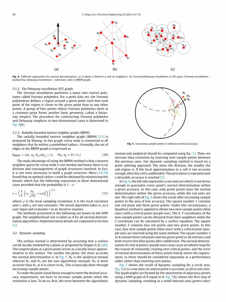

50 T. Song et al. / Precision Engineering 39 (2015) 47–55

Pq1

q2q3

q4

q5

q6

q7

P

q1

q2

q3

q4

q5

q6

(a) (b) (c)

q1

q2

q3

q4

q7

q6

q5

q8

q9 q10

q11q12 q13

q14

F nd its neighbors; (b) Voronoi/Delaunay tessellation in 2D space (Voronoi tessellation –d

3

tpppanaF

3

pne

E

ndifbc

r

wau

gn3

3

cTitwai

rr

N0

N2

N1

V

L1

L2

ig. 4. Different approaches for normal determination: (a) A plane is fitted to p aashed line, Delaunay tessellation – solid line); and (c) RBNN graph.

.1.2. The Delaunay tessellation (DT) graphThe Voronoi tessellation partitions a space into convex poly-

opes called Voronoi polyhedra. For a point data set, the Voronoiolyhedron defines a region around a given point such that eachoint of the region is closer to the given point than to any otheroints. A group of four points whose Voronoi polyhedra meet at

common point forms another basic geometry, called a Delau-ay simplex. The procedure for constructing Voronoi polyhedrand Delaunay simplices in two-dimensional cases is illustrated inig. 4(b).

.1.3. Radially bounded nearest neighbor graph (RBNN)The radially bounded nearest neighbor graph (RBNN) [17] is

roposed by Klasing. In this graph, every node is connected to alleighbors that lie within a predefined radius r. Formally, the set ofdges in the RBNN graph is expressed as

RBNN = {{ui, uj, di,j}|di,j ≤ r}, ∀ui, uj, ∈ U, i /= j (10)

The main advantage of using the RBNN method is that a nearesteighbor query for every node is not needed and hence there is noivision and rearrangement of graph structures involved. In fact,

t is not even necessary to build a graph structure. Mitra [18,19]ound that an optimal radius r could be obtained by minimizing thisound, which has the following expression in three dimensionalases provided that the probability is 1 − ε:

=(

1k

(c1

�n√ε�

+ c2�2n

))1/3(11)

here � is the local sampling resolution, k is the local curvaturend c1 and c2 are two constants. The actual algorithm takes �n as aser input and evaluates r in an iterative manner.

The methods presented in the following are based on the kNNraph. The neighborhood size is taken as 4 for all normal determi-ation algorithms. Implementation details are explained in Section.2.

.2. Dynamic sampling

The surface normal is determined by assuming that a surfacean be locally modeled by a plane as proposed by Hoppe et al. [20].he tangent plane at a given point serves as a locally linear approx-mation to the surface. The smaller the plane, the more accuratehe normal determination is. In Fig. 5, N0 is the analytical normalhereas N1 and N2 are the two algorithmic normals. N2 is more

ccurate than N1 as it is closer to No. This is basically done through

ncreasing sample points.

To make the point cloud dense enough to meet the desired accu-acy requirement, we have to increase sample points when theesolution is low. To do so, first, the error between the algorithmic

Fig. 5. Increasing sample points to enhance normal accuracy.

normal and analytical should be computed using Eq. (1). Then, weincrease data resolution by inserting new sample points betweenthe previous ones. Our dynamic sampling method is based on apoint splitting approach. The more the division, the smaller thesub-region is. If the local approximation in a cell is not accurateenough, then this cell is subdivided. This procedure is repeated untila desirable accuracy is reached [7].

In Fig. 6, the left side represents a raw data set which is not denseenough to guarantee every point’s normal determination withina given accuracy. In this case, only green points have the normaldetermination within the given accuracy, while the red ones arenot. The right side of Fig. 6 shows the result after increasing samplepoints in the area of low accuracy. The square number 1 containsone red point and three green points. Under this circumstance, aQuadtree method is applied to obtain two new sample points (blueones) with a critical point (purple one). The X–Y coordinates of thenew sample points can be obtained from their neighbors while theZ coordinate can be calculated by a surface equation. The squarenumber 2 contains two red points and two green points. In thiscase, four new sample points (blue ones) with a critical point (pur-ple one) are inserted using the same method. The square number 3or 4 contain three red points and one green point or all red ones, andboth receive five blue points after subdivision. The normal determi-nation of critical points (purple ones) may cause an infinite loop forthe reason of constantly creating new critical points, and the errorof normal determination of these points barely meets the require-ment, so these should be considered separately as a performanceindex rather than inserting new points.

Fig. 7 shows the result of dynamic sampling for a circle area.

Fig. 7(a) is a raw data set and no point is accurate, so all in red color.The quadrangles are formed by the attachment of adjacency pointsusing a kNN graph of K equal to 4. Fig. 7(b) shows the first step ofdynamic sampling, resulting in a small internal area (green color)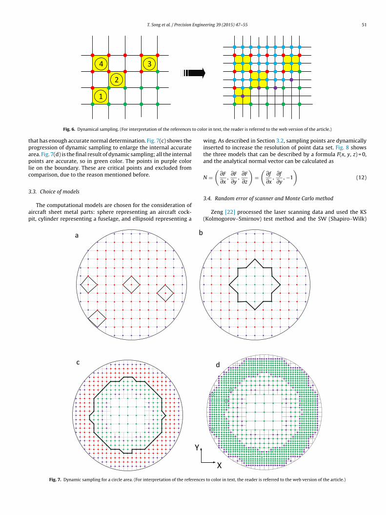

T. Song et al. / Precision Engineering 39 (2015) 47–55 51

1

2

34

to colo

tpaplc

3

ap

Fig. 6. Dynamical sampling. (For interpretation of the references

hat has enough accurate normal determination. Fig. 7(c) shows therogression of dynamic sampling to enlarge the internal accuraterea. Fig. 7(d) is the final result of dynamic sampling; all the internaloints are accurate, so in green color. The points in purple color

ie on the boundary. These are critical points and excluded fromomparison, due to the reason mentioned before.

.3. Choice of models

The computational models are chosen for the consideration ofircraft sheet metal parts: sphere representing an aircraft cock-it, cylinder representing a fuselage, and ellipsoid representing a

a b

c

Y

Fig. 7. Dynamic sampling for a circle area. (For interpretation of the references

r in text, the reader is referred to the web version of the article.)

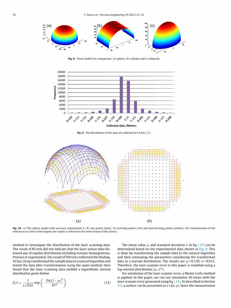
wing. As described in Section 3.2, sampling points are dynamicallyinserted to increase the resolution of point data set. Fig. 8 showsthe three models that can be described by a formula F(x, y, z) = 0,and the analytical normal vector can be calculated as

N =(

∂F

∂x,

∂F

∂y,

∂F

∂z

)=

(∂f

∂x,

∂f

∂y, −1

)(12)

3.4. Random error of scanner and Monte Carlo method

Zeng [22] processed the laser scanning data and used the KS(Kolmogorov–Smirnov) test method and the SW (Shapiro–Wilk)

X

d

to color in text, the reader is referred to the web version of the article.)

52 T. Song et al. / Precision Engineering 39 (2015) 47–55

Fig. 8. Three models for comparison: (a) sphere, (b) cylinder and (c) ellipsoid.

Freq

uenc

y

02000400060008000

100001200014000160001800020000

Collected data /M eter s

Fig. 9. The distribution of the data set collected in 0.14 m [22].

F , 1st ir ticle.)

mTlPAtfd

f

ig. 10. (a) The sphere model with accuracy requirement 2; (b) raw points (dark)eferences to color in this legend, the reader is referred to the web version of the ar

ethod to investigate the distribution of the laser scanning data.he result of KS test did not indicate that the laser sensor data fol-owed any of regular distribution including normal, homogeneous,oisson or exponential. The result of SW test confirmed this finding.t last, Zeng transformed the sample data to a natural logarithm and

ested the data after transformation using the same method, thenound that the laser scanning data yielded a logarithmic normal

istribution given below

(z) = 1

z√

2��exp

(− (ln(z) − �)2

2�2

)(13)

nserting points (red) and 2nd inserting points (yellow). (For interpretation of the

The mean value � and standard deviation � in Eq. (13) can bedetermined based on the experimental data shown in Fig. 9. Thisis done by transforming the sample data to the natural logarithmand then estimating the parameters considering the transformeddata in a normal distribution. The results are � = 0.139, � = 0.012.Therefore, the laser scanner error in this paper is modeled using alog-normal distribution (�, �2).

For simulation of the laser scanner error, a Monte Carlo methodis applied. In this paper, we run our simulation 50 times with thelaser scanner error generated using Eq. (13). As described in Section3.3, a surface can be presented as z = f(x, y). Since the measurement

T. Song et al. / Precision Engineering 39 (2015) 47–55 53

Table 1The sizes of the models (mm).

Model Sphere Cylinder Ellipsoid

Model 1 Radius = 10,000 a = 5000;b = 5000;c = 10,000;

Radius = 10,000

Model 2 Radius = 5000 a = 2500;b = 2500;c = 5000;

Radius = 5000

Model 3 Radius = 1000 a = 500; Radius = 1000

ed

3

kpoetuieat

(((

4

agaatoarpmrc

0

0.5

1

1.5

2

2.5

3

3.5

MWE MWA MW SELR MW AAT MWE LR MW RELR

Ave Tim e

TT

b = 500;c = 1000;

rror is modeled as z∼ log N(�, �2) − 0.14, the actual simulatedata set z′ is obtained as z′ = z + z.

.5. Performance indices

As stated in Section 3.2, the method of dynamic sampling is toeep increasing the resolution of a point date set after each com-utation till the required accuracy is met. First, the total numberf final data points should be evaluated as it indicates how heavilyach algorithm relies on the characteristics of the model. Second,he number of times needed to increase the data resolution (calledp-sampling) is another important factor to compare, which could

ndicate how sensitive each algorithm is to different models andrrors. The last item that should be compared is computing time,s our study is intended for real-time application. To summarize,he following performance indices are used for comparison.

1) Total number of points.2) The number of times of up-sampling.3) Computing time.

. Results

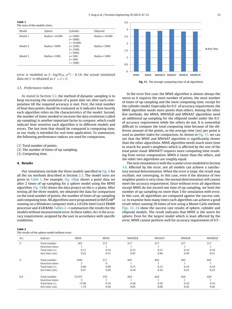
Our simulations include the three models specified in Fig. 6 forll the six methods described in Section 2.2. The model sizes areiven in Table 1. For example, Fig. 10(a) shows a point data setfter 2 times of up-sampling for a sphere model using the MWElgorithm. Fig. 10(b) shows the data project on the x–y plane. Afteresting all the three models, we obtained the data for comparisonn the total number of points, the number of times of up-samplingnd computing time. All algorithms were programmed in MATLAB®

unning on a Windows computer with a 3.0 GHz Intel Core2 E8400

rocessor and 4 GB RAM. Tables 2–4 summarizes the results for theodels without measurement error. In these tables, Acc is the accu-

acy requirement, assigned by the user in accordance with specificonditions.

able 2he results of the sphere model without error.

Acc Indexes MWE MWA

5◦ Total number 501 317

Insertion times 1 1

Total time (s) 0.11 0.10

Ave time (ms) 0.22 0.31

2◦ Total number 1445 317

Insertion times 2 0

Total time (s) 0.40 0.09

Ave time (ms) 0.27 0.29

0.5◦ Total number 15,557 376

Insertion times 5 1

Total time (s) 17.06 0.16

Ave time (ms) 1.10 0.44

Fig. 11. The average computing time of all algorithms.

In the error free case, the MWE algorithm is almost always theworst as it requires the most number of points, the most numberof times of up-sampling and the most computing time, except forthe cylinder model. Especially for 0.5◦ of accuracy requirement, theMWE algorithm needs more points than others. Among the otherfive methods, the MWA, MWSELR and MWAAT algorithms needan additional up-sampling for the ellipsoid model under the 0.5◦

of accuracy requirement while the others do not. It is somewhatdifficult to compare the total computing time because of the dif-ferent amount of the points, so the average time (ms) per point isused as another index for comparison. As shown in Fig. 11, we cansee that the MWE and MWAAT algorithm is significantly slowerthan the other algorithms. MWE algorithm needs much more timeto search for point’s neighbors which is affected by the size of thetotal point cloud. MWAATT requires more computing time result-ing from vector computation. MWA is faster than the others, andthe other two algorithms are roughly equal.

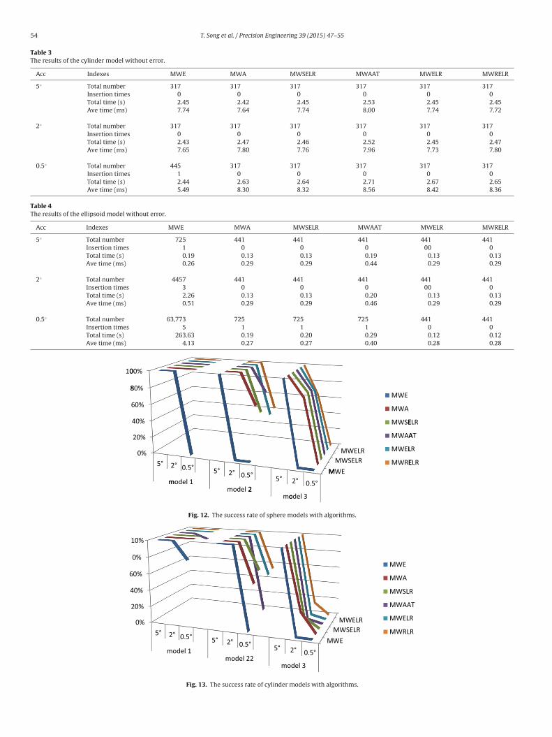
The next simulation is with the scanner error modeled in Section3.4. Affected by the error, not all models can achieve a satisfac-tory normal determination. When the error is large, the result mayoscillate, not converging. In this case, even if the distance of twoneighbor points is very close, the normal determination still cannotmeet the accuracy requirement. Since without error all algorithmsexcept MWE do not exceed one time of up-sampling, we limit thenumber of up-sampling no more than 3 for simulation with error.In this case, all algorithms are compared against the success rate,i.e. to examine how many times each algorithm can achieve a goodresult when running 50 times of test using a Monte Carlo method.Figs. 12–14 show the success rate results of sphere, cylinder and

ellipsoid models. The result indicates that MWE is the worst forsphere. Even for the largest model which is least affected by theerror, MWE cannot perform well for accuracy requirement of 0.5◦.

MWSELR MWAAT MWELR MWRELR

317 317 317 3171 1 1 10.15 0.15 0.10 0.100.47 0.46 0.30 0.31

445 445 445 4451 1 1 10.15 0.15 0.10 0.100.34 0.34 0.23 0.23

424 424 424 4241 1 1 10.28 0.29 0.19 0.190.65 0.66 0.45 0.45

54 T. Song et al. / Precision Engineering 39 (2015) 47–55

Table 3The results of the cylinder model without error.

Acc Indexes MWE MWA MWSELR MWAAT MWELR MWRELR

5◦ Total number 317 317 317 317 317 317Insertion times 0 0 0 0 0 0Total time (s) 2.45 2.42 2.45 2.53 2.45 2.45Ave time (ms) 7.74 7.64 7.74 8.00 7.74 7.72

2◦ Total number 317 317 317 317 317 317Insertion times 0 0 0 0 0 0Total time (s) 2.43 2.47 2.46 2.52 2.45 2.47Ave time (ms) 7.65 7.80 7.76 7.96 7.73 7.80

0.5◦ Total number 445 317 317 317 317 317Insertion times 1 0 0 0 0 0Total time (s) 2.44 2.63 2.64 2.71 2.67 2.65Ave time (ms) 5.49 8.30 8.32 8.56 8.42 8.36

Table 4The results of the ellipsoid model without error.

Acc Indexes MWE MWA MWSELR MWAAT MWELR MWRELR

5◦ Total number 725 441 441 441 441 441Insertion times 1 0 0 0 00 0Total time (s) 0.19 0.13 0.13 0.19 0.13 0.13Ave time (ms) 0.26 0.29 0.29 0.44 0.29 0.29

2◦ Total number 4457 441 441 441 441 441Insertion times 3 0 0 0 00 0Total time (s) 2.26 0.13 0.13 0.20 0.13 0.13Ave time (ms) 0.51 0.29 0.29 0.46 0.29 0.29

0.5◦ Total number 63,773 725 725 725 441 441Insertion times 5 1 1 1 0 0Total time (s) 263.63 0.19 0.20 0.29 0.12 0.12Ave time (ms) 4.13 0.27 0.27 0.40 0.28 0.28

8

10

0%

20%

40%

60%

80%

00%

5°

m

2° 0.5°

model 15° 2° 0.5°

mod el 25°

2mo

M2° 0.5°

odel 3

MWEMWSELR

MWELR

MWE

MWA

MWS E

MWA A

MWE L

MWR E

ELR

AT

LR

ELR

Fig. 12. The success rate of sphere models with algorithms.

10%

0%

20%

40%

60%

0%

5° 2° 0.5°

model 15° 2° 0.5°

model 225°

model 3

M2° 0.5°

WEMWSELR

MWELR

MWE

MWA

MWS LR

MWAA T

MWEL R

MWRLR

Fig. 13. The success rate of cylinder models with algorithms.

T. Song et al. / Precision Engineering 39 (2015) 47–55 55

8

10

0%

20%

40%

60%

80%

0%

5°

m

2° 0.5°

model 15° 2° 0.5°

mod el 25°

M2° 0.5°

WEMWSELR

MWELR

MWE

MWA

MWSE

MWAA

MWEL

MWRE

LR

T

R

LR

ellipso

MMtodtrs

5

barotMnTMa

A

TaR

R

[

[

[

[

[

[

[

[

[

[

[

conference on computer graphics and interactive techniques. 1992. p. 71–8.

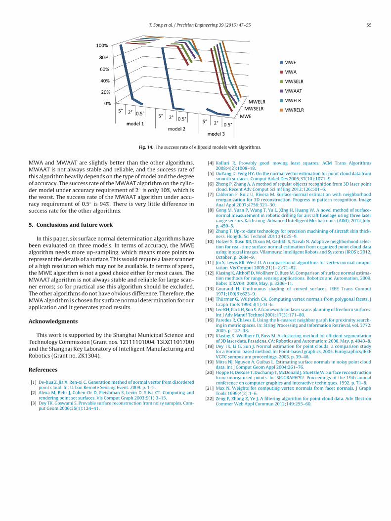
Fig. 14. The success rate of

WA and MWAAT are slightly better than the other algorithms.WAAT is not always stable and reliable, and the success rate of

his algorithm heavily depends on the type of model and the degreef accuracy. The success rate of the MWAAT algorithm on the cylin-er model under accuracy requirement of 2◦ is only 10%, which ishe worst. The success rate of the MWAAT algorithm under accu-acy requirement of 0.5◦ is 94%. There is very little difference inuccess rate for the other algorithms.

. Conclusions and future work

In this paper, six surface normal determination algorithms haveeen evaluated on three models. In terms of accuracy, the MWElgorithm needs more up-sampling, which means more points toepresent the details of a surface. This would require a laser scannerf a high resolution which may not be available. In terms of speed,he MWE algorithm is not a good choice either for most cases. The

WAAT algorithm is not always stable and reliable for large scan-er errors; so for practical use this algorithm should be excluded.he other algorithms do not have obvious difference. Therefore, theWA algorithm is chosen for surface normal determination for our

pplication and it generates good results.

cknowledgments

This work is supported by the Shanghai Municipal Science andechnology Commission (Grant nos. 12111101004, 13DZ1101700)nd the Shanghai Key Laboratory of Intelligent Manufacturing andobotics (Grant no. ZK1304).

eferences

[1] De-hua Z, Jia X, Ren-xi C. Generation method of normal vector from disordered

point cloud. In: Urban Remote Sensing Event. 2009. p. 1–5.

[2] Alexa M, Behr J, Cohen-Or D, Fleishman S, Levin D, Silva CT. Computing andrendering point set surfaces. Vis Comput Graph 2003;9(1):3–15.

[3] Dey TK, Goswami S. Provable surface reconstruction from noisy samples. Com-put Geom 2006;35(1):124–41.

[

[

moodel 3

id models with algorithms.

[4] Kolluri R. Provably good moving least squares. ACM Trans Algorithms2008;4(2):1008–18.

[5] OuYang D, Feng HY. On the normal vector estimation for point cloud data fromsmooth surfaces. Comput Aided Des 2005;37(10):1071–9.

[6] Zheng P, Zhang A. A method of regular objects recognition from 3D laser pointcloud. Recent Adv Comput Sci Inf Eng 2012;126:501–6.

[7] Calderon F, Ruiz U, Rivera M. Surface-normal estimation with neighborhoodreorganization for 3D reconstruction. Progress in pattern recognition. ImageAnal Appl 2007;4756:321–30.

[8] Gong M, Yuan P, Wang T, Yu L, Xing H, Huang W. A novel method of surface-normal measurement in robotic drilling for aircraft fuselage using three laserrange sensors. Kachsiung: Advanced Intelligent Mechatronics (AIM); 2012, July.p. 450–5.

[9] Zhang T. Up-to-date technology for precision machining of aircraft skin thick-ness. Hongdu Sci Technol 2011;(4):25–9.

10] Holzer S, Rusu RB, Dixon M, Gedikli S, Navab N. Adaptive neighborhood selec-tion for real-time surface normal estimation from organized point cloud datausing integral images. Vilamoura: Intelligent Robots and Systems (IROS); 2012,October. p. 2684–9.

11] Jin S, Lewis RR, West D. A comparison of algorithms for vertex normal compu-tation. Vis Comput 2005;21(1–2):71–82.

12] Klasing K, Althoff D, Wollherr D, Buss M. Comparison of surface normal estima-tion methods for range sensing applications. Robotics and Automation, 2009.Kobe: ICRA’09; 2009, May. p. 3206–11.

13] Gouraud H. Continuous shading of curved surfaces. IEEE Trans Comput1971;100(6):623–9.

14] Thürrner G, Wüthrich CA. Computing vertex normals from polygonal facets. JGraph Tools 1998;3(1):43–6.

15] Lee KH, Park H, Son S. A framework for laser scans planning of freeform surfaces.Int J Adv Manuf Technol 2001;17(3):171–80.

16] Paredes R, Chávez E. Using the k-nearest neighbor graph for proximity search-ing in metric spaces. In: String Processing and Information Retrieval, vol. 3772.2005. p. 127–38.

17] Klasing K, Wollherr D, Buss M. A clustering method for efficient segmentationof 3D laser data. Pasadena, CA: Robotics and Automation; 2008, May. p. 4043–8.

18] Dey TK, Li G, Sun J. Normal estimation for point clouds: a comparison studyfor a Voronoi based method. In: Point-based graphics, 2005. Eurographics/IEEEVGTC symposium proceedings. 2005. p. 39–46.

19] Mitra NJ, Nguyen A, Guibas L. Estimating surface normals in noisy point clouddata. Int J Comput Geom Appl 2004:261–76.

20] Hoppe H, DeRose T, Duchamp T, McDonald J, Stuetzle W. Surface reconstructionfrom unorganized points. In: SIGGRAPH’92. Proceedings of the 19th annual

21] Max N. Weights for computing vertex normals from facet normals. J GraphTools 1999;4(2):1–6.

22] Zeng F, Zhong Z, Ye J. A filtering algorithm for point cloud data. Adv ElectronCommer Web Appl Commun 2012;149:255–60.