A comparison of fractal dimension estimators based on multiple surface generation algorithms

$Page 1: A comparison of fractal dimension estimators based on multiple surface generation algorithms$
ARTICLE IN PRESS

0098-3004/$ - se

doi:10.1016/j.ca

�Correspondfax: 1 225 578 44

E-mail addr

Computers & Geosciences 31 (2005) 1260–1269

www.elsevier.com/locate/cageo

A comparison of fractal dimension estimators based onmultiple surface generation algorithms

Guiyun Zhou�, Nina S.-N. Lam

Department of Geography and Anthropology, Louisiana State University, Baton Rouge, LA 70803, USA

Received 12 November 2004; received in revised form 22 March 2005; accepted 22 March 2005

Abstract

Fractal geometry has been actively researched in a variety of disciplines. The essential concept of fractal analysis is

fractal dimension. It is easy to compute the fractal dimension of truly self-similar objects. Difficulties arise, however,

when we try to compute the fractal dimension of surfaces that are not strictly self-similar. A number of fractal surface

dimension estimators have been developed. However, different estimators lead to different results. In this paper, we

compared five fractal surface dimension estimators (triangular prism, isarithm, variogram, probability, and variation)

using surfaces generated from three surface generation algorithms (shear displacement, Fourier filtering, and midpoint

displacement). We found that in terms of the standard deviations and the root mean square errors, the triangular prism

and isarithm estimators perform the best among the five methods studied.

r 2005 Elsevier Ltd. All rights reserved.

Keywords: Fractal dimension estimator; Fractal Brownian motion; Surface generation algorithms

1. Introduction

Fractal geometry is a useful way to describe and

characterize complex shapes and surfaces. Recent

research in geosciences and environmental science

communities have pushed the use of fractals into the

realm of metadata representation, environmental mon-

itoring, change detection, and landscape and feature

characterization (e.g., Lam, 2004; Lam et al., 1998;

Quattrochi et al., 2001; Read and Lam, 2002; Al-

Hamdan, 2004). The idea of fractal geometry was

originally derived by Mandelbrot in 1967 to describe

self-similar geometric figures such as the von Koch curve

(Mandelbrot, 1967, 1983). Fractal dimension (D) is a

key quantity in fractal geometry. The D value can be a

e front matter r 2005 Elsevier Ltd. All rights reserve

geo.2005.03.016

ing author. Tel.: +1225 578 6119;

20.

ess: [email protected] (G. Zhou).

non-integer and can be used as an indicator of the

complexity of curves and surfaces. For a self-similar

figure, it can be decomposed into N small parts, where

each part is a reduced copy of the original figure by a

ratio r. The D of a self-similar figure can be defined as

D ¼ � logðNÞ= logðrÞ (Mandelbrot, 1967). For curves

and images that are not self-similar, there exist

numerous empirical methods to compute D. Results

from different estimators were found to differ from each

other (Klinkenberg and Goodchild, 1992). This is

partly due to the elusive definition of D, i.e., the

Hausdorff–Besicovitch dimension (Tate, 1998). For

results to be comparable and D be useful for the

characterization of textures, we need a robust estimator

that can give an estimate that, on the one hand, agrees

with our intuition of the complexity of curves and

surfaces, and, on the other hand, provides the best

discriminating ability among curves and surfaces of

different complexity.

d.

www.elsevier.com/locate/cageo

ARTICLE IN PRESS

A

CD

P

E

X

Y

Z

B

Fig. 1. Triangular prism.

G. Zhou, N.S.-N. Lam / Computers & Geosciences 31 (2005) 1260–1269 1261

This paper compared five methods for calculating the

D of a raster image, including the triangular prism,

isarithm, variogram, probability, and variation estima-

tors. We used benchmark surfaces of known D values

generated from three algorithms, which include the shear

displacement, Fourier filtering, and midpoint displace-

ment methods. Similar studies that compared fractal

estimators have been conducted before. Klinkenberg and

Goodchild (1992) tested seven methods on 55 real

topographic data sets that yielded mixed results. Tate

(1998) analyzed several estimators using nine simulated

surfaces and also found that different estimators led to

different results. Using 25 simulated surfaces, Lam et al.

(2002) compared the first three estimators and found that

the isarithm and the triangular prism estimators generally

performed better than the variogram estimator. All these

previous studies provided useful information but also

pointed to the need for further research with a variety of

data. This study will add to the fractal literature by

comparing two additional fractal surface dimension

estimators using a total of 750 surfaces generated from

three different algorithms. Surfaces generated from

multiple algorithms are helpful to check whether the

estimators respond consistently when applied to images

from different sources, such as remote sensing images

acquired from disparate satellite platforms. Through this

large-scale experiment, we hope to provide more con-

fidence of our results and a better understanding of the

selected fractal surface estimators.

2. Estimators of D of an image

There are numerous methods proposed to calculate

the D of an image. In this paper, we studied five D

estimators, i.e., triangular prism, isarithm, variogram,

probability, and variation estimators. Computer pro-

grams for the first three estimators are available in

Image Characterization And Measurement System

(ICAMS), a software designed to compute fractal

dimension and other spatial indices for multi-scale

remote sensing data (Quattrochi et al., 1997; Lam

et al., 1998). The probability and variation estimators

were programmed in C++ for this study. Flowcharts

and algorithms for the first three methods have been

documented in Jaggi et al. (1993) and Lam and De Cola

(1993, 2002), and therefore will only be briefly described

in this paper. The latter two methods were newly added

and their algorithms will be described in more detail

below. Both ICAMS and the additional programs for

this study are available from the authors.

2.1. Triangular prism

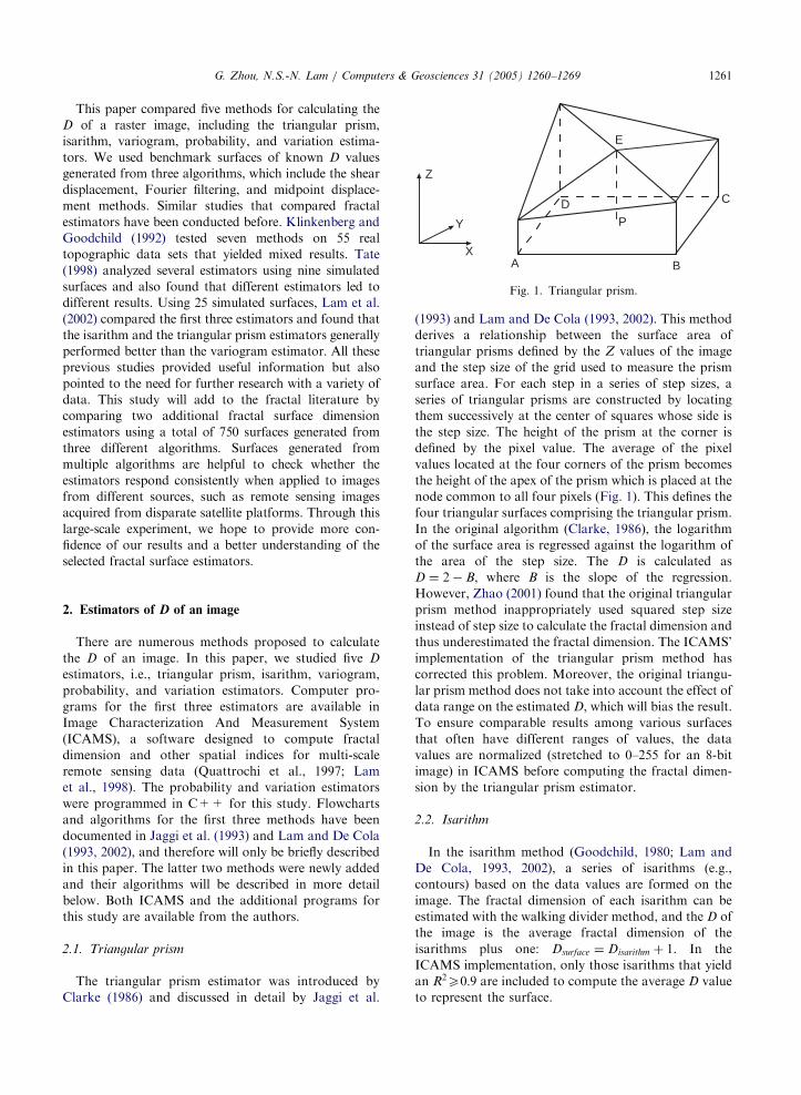
The triangular prism estimator was introduced by

Clarke (1986) and discussed in detail by Jaggi et al.

(1993) and Lam and De Cola (1993, 2002). This method

derives a relationship between the surface area of

triangular prisms defined by the Z values of the image

and the step size of the grid used to measure the prism

surface area. For each step in a series of step sizes, a

series of triangular prisms are constructed by locating

them successively at the center of squares whose side is

the step size. The height of the prism at the corner is

defined by the pixel value. The average of the pixel

values located at the four corners of the prism becomes

the height of the apex of the prism which is placed at the

node common to all four pixels (Fig. 1). This defines the

four triangular surfaces comprising the triangular prism.

In the original algorithm (Clarke, 1986), the logarithm

of the surface area is regressed against the logarithm of

the area of the step size. The D is calculated as

D ¼ 2� B, where B is the slope of the regression.

However, Zhao (2001) found that the original triangular

prism method inappropriately used squared step size

instead of step size to calculate the fractal dimension and

thus underestimated the fractal dimension. The ICAMS’

implementation of the triangular prism method has

corrected this problem. Moreover, the original triangu-

lar prism method does not take into account the effect of

data range on the estimated D, which will bias the result.

To ensure comparable results among various surfaces

that often have different ranges of values, the data

values are normalized (stretched to 0–255 for an 8-bit

image) in ICAMS before computing the fractal dimen-

sion by the triangular prism estimator.

2.2. Isarithm

In the isarithm method (Goodchild, 1980; Lam and

De Cola, 1993, 2002), a series of isarithms (e.g.,

contours) based on the data values are formed on the

image. The fractal dimension of each isarithm can be

estimated with the walking divider method, and the D of

the image is the average fractal dimension of the

isarithms plus one: Dsurface ¼ Disarithm þ 1. In the

ICAMS implementation, only those isarithms that yield

an R2X0:9 are included to compute the average D value

to represent the surface.

ARTICLE IN PRESSG. Zhou, N.S.-N. Lam / Computers & Geosciences 31 (2005) 1260–12691262

2.3. Variogram

The variogram estimator (Mark and Aronson, 1984;

Jaggi et al., 1993; Lam and De Cola, 1993) measures D

of an image based on the variogram computed for the

study area, and gðhÞ ¼ VarðZi � ZjÞ, where i; j are

spaced by the distance vector h. The D can be derived

by regressing the logarithm of the distance vector with

the logarithm of the variance, and D ¼ 3� ðB=2Þ, whereB is the slope of the regression.

2.4. Probability

Voss (1988) proposed a method to compute the fractal

dimension. Let P(m, L) be the probability that there are

m points within a cube with side length L centered on an

arbitrary point in an image. Let N be the maximum

number of possible points in the cube. Let NðLÞ ¼

PNm¼1

1=mPðm;LÞ, then NðLÞ / 1=LD. D ¼ �B, where B is

the slope of the regression of log(N(L)) versus log(L).

P(m, L) is estimated from the image data. In our

implementation, P(m, L) is estimated as follows. Each

pixel in the image is treated as a point in the three-

dimensional space. The coordinates of each pixel are its

row and column values in the two-dimensional image

space and the pixel value in the third (z) dimension. A

cube with side length L (an odd number) is centered on

each point successively except those points along the side

on which the cube extends outside the boundary of the

image. The algorithm will determine how many m points

are in each box using the criterion:

z �L � 1

2; z þ

L � 1

2

� �,

Selected area (top, left, bottom, right)number_ of_ steps

step

for eacfor e

Center the box (cube) on pixel (row,col)compute the number of points (m) falling in the box

End of iteration?

Compute P(m, L) from the relative frequency of boxes containing m number of points

Do a regression of log(N(L)) versus log (L)Fractal dimension = - slope of gressionEnd

Yes

N

Fig. 2. Flowchart of pro

where z is the value of the center pixel. If only one pixel

within the box has a value within the range, then m ¼ 1,

and vice versa. The algorithm will then tabulate how

many boxes of size L has m ¼ 1, 2, 3, and so on. m is no

less than one since the center pixel is always in the cube.

P(m, L) is calculated as a ratio of the number of cubes of

size L with a value of m and the total number of boxes of

size L. The flowchart to compute the fractal dimension

using the probability method is shown in Fig. 2.

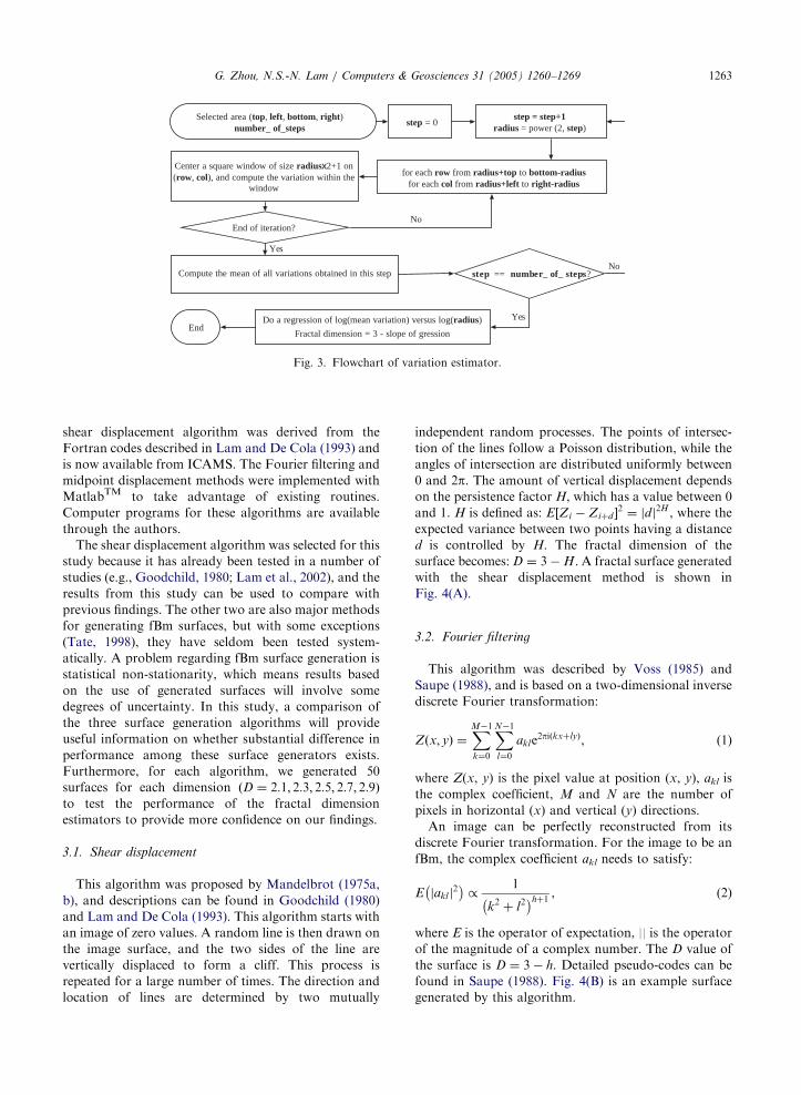
2.5. Variation

The variation estimator is computed in the following

manner (Parker, 1997; Tolle et al., 2003). Fig. 3 shows

the flowchart to compute the D by this method. An odd-

number moving window (e.g., 3� 3, 5� 5) of side length

L is placed over each point to compute the variation of

the z values within the window, where L is determined

by the radius � : L ¼ 2�þ 1. Variation is defined as the

difference between the maximum pixel value and the

minimum value within the window. After the window

moves to the last point, the mean variation is computed

to form V ð�Þ. By varying �, we will get corresponding

Vð�Þ. The fractal dimension is given as D ¼ 3� B, where

B is the slope of the regression of logV ð�Þ versus log �.

3. Surface generation algorithms

Natural objects can seldom be strictly self-similar;

most of them can at best be considered statistically self-

similar. One mathematical model to describe this

random fractal is fractional Brownian motion (fBm)

(Mandelbrot, 1983). There are a few surface generation

algorithms available to generate approximations to fBm

surfaces. In this paper, we studied three of them. The

= 0step = step+1

half_size = power (2, step)L = 2xhalf_size+1

h row from half_size+top to bottom-half_sizeach col from half_size+left to right-half_size

1

NCompute N(L) = 1/ mp(m,L)

step == number_ of_ steps?NoYes

o

∑

bability estimator.

ARTICLE IN PRESS

Selected area (top, left, bottom, right)number_ of_steps

step = 0step = step+1

radius = power (2, step)

for each row from radius+top to bottom-radiusfor each col from radius+left to right-radius

Center a square window of size radiusx2+1 on(row, col), and compute the variation within the

window

End of iteration?

Compute the mean of all variations obtained in this step

Do a regression of log(mean variation) versus log(radius)

Fractal dimension = 3 - slope of gressionEnd

Yes

step == number_ of_ steps?No

Yes

No

Fig. 3. Flowchart of variation estimator.


shear displacement algorithm was derived from the

Fortran codes described in Lam and De Cola (1993) and

is now available from ICAMS. The Fourier filtering and

midpoint displacement methods were implemented with

MatlabTM to take advantage of existing routines.

Computer programs for these algorithms are available

through the authors.

The shear displacement algorithm was selected for this

study because it has already been tested in a number of

studies (e.g., Goodchild, 1980; Lam et al., 2002), and the

results from this study can be used to compare with

previous findings. The other two are also major methods

for generating fBm surfaces, but with some exceptions

(Tate, 1998), they have seldom been tested system-

atically. A problem regarding fBm surface generation is

statistical non-stationarity, which means results based

on the use of generated surfaces will involve some

degrees of uncertainty. In this study, a comparison of

the three surface generation algorithms will provide

useful information on whether substantial difference in

performance among these surface generators exists.

Furthermore, for each algorithm, we generated 50

surfaces for each dimension ðD ¼ 2:1; 2:3; 2:5; 2:7; 2:9Þto test the performance of the fractal dimension

estimators to provide more confidence on our findings.

3.1. Shear displacement

This algorithm was proposed by Mandelbrot (1975a,

b), and descriptions can be found in Goodchild (1980)

and Lam and De Cola (1993). This algorithm starts with

an image of zero values. A random line is then drawn on

the image surface, and the two sides of the line are

vertically displaced to form a cliff. This process is

repeated for a large number of times. The direction and

location of lines are determined by two mutually

independent random processes. The points of intersec-

tion of the lines follow a Poisson distribution, while the

angles of intersection are distributed uniformly between

0 and 2p. The amount of vertical displacement dependson the persistence factor H, which has a value between 0

and 1. H is defined as: E Zi � Ziþd½ 2 ¼ dj j2H , where the

expected variance between two points having a distance

d is controlled by H. The fractal dimension of the

surface becomes: D ¼ 3� H: A fractal surface generated

with the shear displacement method is shown in

Fig. 4(A).

3.2. Fourier filtering

This algorithm was described by Voss (1985) and

Saupe (1988), and is based on a two-dimensional inverse

discrete Fourier transformation:

Zðx; yÞ ¼XM�1

k¼0

XN�1

l¼0

akle2piðkxþlyÞ, (1)

where Z(x, y) is the pixel value at position (x, y), akl is

the complex coefficient, M and N are the number of

pixels in horizontal (x) and vertical (y) directions.

An image can be perfectly reconstructed from its

discrete Fourier transformation. For the image to be an

fBm, the complex coefficient akl needs to satisfy:

E aklj j2� �

/1

k2þ l2

� �hþ1, (2)

where E is the operator of expectation, || is the operator

of the magnitude of a complex number. The D value of

the surface is D ¼ 3� h. Detailed pseudo-codes can be

found in Saupe (1988). Fig. 4(B) is an example surface

generated by this algorithm.


3.3. Midpoint displacement

This algorithm was proposed by Fournier et al. (1982)

and discussed by Voss (1988) and Saupe (1988). The

algorithm starts with an image with pixel values at four

corners drawn from a Gaussian distribution Nðm; s2Þ. Acenter point (midpoint) is then assigned, and its value is

the average of its four neighboring pixels plus a random

value generated from a Gaussian distribution N m; s2

2h

� �.

This process is repeated until we get the desired number

of pixels. The D value of the surface is D ¼ 3� h. This

algorithm leads to non-stationary simulations. To

mitigate non-stationarity, Voss (1988) further added

random additions to the four neighboring pixels (Tate,

1998). However, our preliminary testing showed that the

random additions added to the neighboring pixels had

little effect on the estimation of fractal dimension. We

thus used the original algorithm, which added random-

Fig. 4. Sample surfaces with a theoretical D of 2.5 generated by (A

displacement.

Table 1

Mean, standard deviation (std), and coefficient of variation (c.v.) of es

shear displacement algorithm

Theoretical D Triangular Isarithm

2.1 mean 2.04 2.04std 0.02 0.13c.v. 0.01 0.06

2.3 mean 2.05 2.09std 0.01 0.02c.v. 0.01 0.01

2.5 mean 2.30 2.39std 0.03 0.02c.v. 0.01 0.01

2.7 mean 2.69 2.78std 0.01 0.02c.v. 0.00 0.01

2.9 mean 2.88 2.95std 0.01 0.03c.v. 0.00 0.01

ness to the midpoint only. Fig. 4(C) shows a surface

generated from this algorithm.

4. Results and discussion

Fifty surfaces of size 513� 513 were generated for

each surface generation algorithm for each of the

following D values: 2.1, 2.3, 2.5, 2.7, and 2.9, resulting

in a total of 750 surfaces. For the shear displacement

algorithm, we used 3000 cuts. The pixel values in all

generated images were linearly rescaled to the range of

0–255. For the triangular prism estimator, we used five

geometric steps. For the isarithm estimator, the isarithm

interval was ten, the number of walking divider steps

was five, and calculations were done along both row and

column directions. For the variogram estimator, we

took systematic sampling by sampling every tenth pixel.

) shear displacement, (B) fourier filtering, and (C) midpoint

timated D’s of 50 surfaces generated for each theoretical D using

Variogram Probability Variation

2.11 2.00 2.03

0.12 0.01 0.04

0.06 0.01 0.02

2.23 2.02 2.09

0.10 0.02 0.04

0.05 0.01 0.02

2.56 2.25 2.37

0.09 0.04 0.02

0.04 0.02 0.01

2.89 2.54 2.62

0.04 0.01 0.01

0.01 0.00 0.00

3.00 2.61 2.72

0.00 0.00 0.01

0.00 0.00 0.00

ARTICLE IN PRESSG. Zhou, N.S.-N. Lam / Computers & Geosciences 31 (2005) 1260–1269 1265

The distances were classified into 20 groups and the first

eight groups were used in the regression. Both prob-

ability and variation estimators used eight geometric

steps (3, 5, 9, 17, 33, 65, 129, 257).

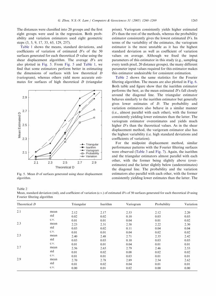
Table 1 shows the means, standard deviations, and

coefficients of variation of estimated D’s of the 50

surfaces generated for each theoretical D value using the

shear displacement algorithm. The average D’s are

also plotted in Fig. 5. From Fig. 5 and Table 1, we

find that some estimators perform better in estimating

the dimensions of surfaces with low theoretical D

(variogram), whereas others yield more accurate esti-

mates for surfaces of high theoretical D (triangular

Table 2


Fourier filtering algorithm


2.1 mean 2.12 2.17std 0.02 0.02c.v. 0.01 0.01

2.3 mean 2.23 2.31std 0.03 0.02c.v. 0.01 0.01

2.5 mean 2.40 2.48std 0.03 0.03c.v. 0.01 0.01

2.7 mean 2.56 2.65std 0.01 0.02c.v. 0.01 0.01

2.9 mean 2.70 2.78std 0.01 0.02c.v. 0.00 0.01

2.1 2.3 2.5 2.7 2.9

2.1

2.3

2.5

2.7

2.9

Theoretical D

Mea

n E

stim

ated

D

TriangularIsarithmVariogramProbabilityVariation

Fig. 5. Mean D of surfaces generated using shear displacement

algorithm.

prism). Variogram consistently yields higher estimated

D’s than the rest of the methods, whereas the probability

estimator consistently gives the lowest estimated D’s. In

terms of the variability of the estimates, the variogram

estimator is the most unstable as it has the highest

standard deviation as well as coefficient of variation

values on average. Although we fixed the input

parameters of this estimator in this study (e.g., sampling

every tenth pixel, 20 distance groups), the many different

parameter input values required for this estimator makes

this estimator undesirable for consistent estimation.

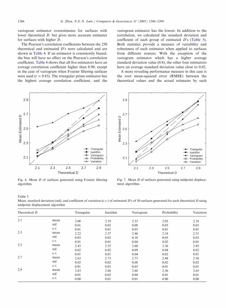
Table 2 shows the same statistics for the Fourier

filtering algorithm. The means are also plotted in Fig. 6.

Both table and figure show that the isarithm estimator

performs the best, as the mean estimated D’s fall closely

around the diagonal line. The triangular estimator

behaves similarly to the isarithm estimator but generally

gives lower estimates of D. The probability and

variation estimators also behave in a similar manner

(i.e., almost parallel with each other), with the former

consistently yielding lower estimates than the latter. The

variogram estimator overestimates and yields much

higher D’s than the theoretical values. As in the shear

displacement method, the varigoram estimator also has

the highest variability (i.e. high standard deviations and

coefficients of variation).

For the midpoint displacement method, similar

performance patterns with the Fourier filtering surfaces

were observed (Table 3 and Fig. 7). Again, the isarithm

and the triangular estimators almost parallel with each

other, with the former being slightly above (over-

estimates) and the latter slightly below (underestimates)

the diagonal line. The probability and the variation

estimators also parallel with each other, with the former

consistently yielding lower estimates than the latter. The



2.53 2.12 2.20

0.10 0.03 0.03

0.04 0.01 0.02

2.58 2.22 2.30

0.11 0.04 0.04

0.04 0.02 0.02

2.71 2.35 2.42

0.10 0.03 0.03

0.04 0.01 0.01

2.79 2.46 2.53

0.08 0.02 0.02

0.03 0.01 0.01

2.89 2.54 2.62

0.04 0.01 0.01

0.02 0.00 0.00


variogram estimator overestimates for surfaces with

lower theoretical D, but gives more accurate estimates

for surfaces with higher D.

The Pearson’s correlation coefficients between the 250

theoretical and estimated D’s were calculated and are

shown in Table 4. If an estimator is consistently biased,

the bias will have no effect on the Pearson’s correlation

coefficient. Table 4 shows that all five estimators have an

average correlation coefficient higher than 0.90, except

in the case of variogram when Fourier filtering surfaces

were used (r ¼ 0:83). The triangular prism estimator has

the highest average correlation coefficient, and the

Table 3


midpoint displacement algorithm


2.1 mean 2.08 2.19std 0.01 0.02c.v. 0.01 0.01

2.3 mean 2.22 2.37std 0.03 0.02c.v. 0.01 0.01

2.5 mean 2.43 2.55std 0.02 0.02c.v. 0.01 0.01

2.7 mean 2.63 2.73std 0.02 0.02c.v. 0.01 0.01

2.9 mean 2.83 2.88std 0.01 0.02c.v. 0.00 0.01

2.1 2.3 2.5 2.7 2.9

2.1

2.3

2.5

2.7

2.9

Theoretical D

Mea

n E

stim

ated

D


Fig. 6. Mean D of surfaces generated using Fourier filtering

algorithm.

variogram estimator has the lowest. In addition to the

correlation, we calculated the standard deviation and

coefficient of each group of estimated D’s (Table 5).

Both statistics provide a measure of variability and

robustness of each estimator when applied to surfaces

from different sources. With the exception of the

variogram estimator which has a higher average

standard deviation value (0.8), the other four estimators

have an average standard deviation value close to 0.02.

A more revealing performance measure in this case is

the root mean-squared error (RMSE) between the

theoretical values and the actual estimates by each



2.33 2.05 2.18

0.08 0.03 0.03

0.03 0.01 0.01

2.46 2.18 2.31

0.10 0.05 0.03

0.04 0.02 0.01

2.60 2.36 2.45

0.09 0.04 0.02

0.04 0.02 0.01

2.73 2.48 2.56

0.08 0.02 0.02

0.03 0.01 0.01

2.88 2.56 2.65

0.04 0.01 0.01

0.01 0.00 0.00

2.1 2.3 2.5 2.7 2.9

2.1

2.3

2.5

2.7

2.9

Theoretical D

Mea

n E

stim

ated

D


Fig. 7. Mean D of surfaces generated using midpoint displace-

ment algorithm.

ARTICLE IN PRESS

Table 5

Mean standard deviations for set of D’s

Triangular Isarithm Variogram Probability Variation

Shear displacement 0.02 0.04 0.07 0.02 0.02Fourier filtering 0.02 0.02 0.09 0.03 0.03Midpoint displacement 0.02 0.02 0.08 0.03 0.02Average 0.02 0.03 0.08 0.02 0.02

Table 4

Pearson’s correlation coefficient between 250 theoretical D’s and measured D’s for each surface generation algorithm


Shear displacement 0.96 0.96 0.96 0.96 0.98Fourier filtering 0.99 0.99 0.83 0.98 0.98Midpoint displacement 1.00 1.00 0.93 0.98 0.99

Average 0.99 0.98 0.90 0.97 0.98

Table 6

RMSE of D’s


Shear displacement 0.06 0.14 0.12 0.10 0.08

0.25 0.21 0.12 0.28 0.21

0.20 0.11 0.11 0.25 0.13

0.02 0.08 0.19 0.16 0.08Average 0.02 0.06 0.10 0.29 0.18

Fourier filtering 0.11 0.12 0.13 0.22 0.14

0.03 0.07 0.44 0.04 0.11

0.07 0.03 0.30 0.09 0.04

0.11 0.03 0.23 0.15 0.08

0.14 0.06 0.12 0.24 0.17Average 0.20 0.12 0.05 0.36 0.28

Midpoint displacement 0.11 0.06 0.23 0.18 0.13

0.02 0.09 0.24 0.06 0.08

0.08 0.07 0.19 0.13 0.03

0.08 0.06 0.13 0.15 0.05

0.07 0.03 0.08 0.22 0.14

0.07 0.03 0.04 0.34 0.25Average 0.06 0.06 0.14 0.18 0.11

Grand average 0.09 0.08 0.16 0.19 0.13


estimator for each theoretical D, which is shown in

Table 6. Both the triangular prism and isarithm

estimators have lower RMSE than the other, meaning

that their estimated D’s are closer to the theoretical

values. Although the probability and variation

estimators are generally stable and correspond linearly

with the theoretical values (as indicated by their

correlation coefficients), their large RMSE values

indicate their inability to yield estimated D’s that

resemble the theoretical D’s. This could indicate a

redefinition of the algorithms such that their estimates

can be shifted up consistently to give better estimates.

The variogram estimator behaves quite erratically and

has the highest RMSE when Fourier filtering surfaces


were used. Finally, we observe that RMSE’s are the

lowest when surfaces generated from the midpoint

displacement method were used, which is an interesting

and unexpected result, as previous research seems to

focus more on the shear displacement algorithm. The

findings from this study regarding the first three

estimators (triangular prism, isarithm, and variogram)

agree with previous studies in which the variogram

estimator was found not suitable for deriving reliable D

values.

5. Conclusions

A number of methods have been proposed to

calculate the fractal dimension of an image. Unfortu-

nately, previous studies show that different methods

often produce different results. In this paper, we studied

and compared five methods for the estimation of fractal

dimensions of two-dimensional surfaces using 750

artificial surfaces generated from three different surface

generation algorithms. Our findings reveal several

important points. First, our results clearly show that

the triangular prism and isarithm estimators perform the

best, as both their RMSE’s and standard deviations are

among the lowest. The variogram estimator is the most

unstable and inaccurate. Second, the probability and

variation estimators behave in a very similar manner

(parallel with each other), with the probability

estimator consistently yielding a lower D estimate

and thus a higher RMSE. Since their correlation

coefficients between estimated and theoretical D’s are

as high as those of the triangular prism and isarithm

estimator, it is possible for future studies that a

redefinition of these two algorithms will lead to

significant improvement in their performance. Third,

our findings show that surfaces generated from the

midpoint displacement algorithm are most agreeable

with the estimated D’s derived from the estimators, as

evidenced from the low RMSE’s and high correlation

coefficients. This is an unexpected but interesting result,

as previous research has been focusing more on

the shear displacement method. Perhaps more use of

the midpoint displacement method is warranted in the

future. Last but not the least, statistics from this

study (the mean standard deviation) can possibly be

used to test the significance of difference between two

measured D’s.

References

Al-Hamdan, M., 2004. Flow resistance characterization of

forested flood plains using spatial analysis of remotely

sensed data and GIS. Ph.D. Dissertation, University of

Alabama-Hunstville, Huntsville, AL, 259pp.

Clarke, K.C., 1986. Computaton of the fractal dimension of

topographic surfaces using the triangular prism surface area

method. Computers & Geosciences 12 (5), 713–722.

Fournier, A., Fussell, D., Carpenter, L., 1982. Computer

rendering of stochastic models. Communications of the

ACM 25 (6), 371–384.

Goodchild, M.F., 1980. Fractals and the accuracy of geogra-

phical measures. Mathematical Geology 12, 85–98.

Jaggi, S., Quattrochi, D.A., Lam, N.S.-N., 1993. Implementa-

tion and operation of three fractal measurement algorithms

for analysis of remote-sensing data. Computers & Geos-

ciences 19 (6), 745–767.

Klinkenberg, B., Goodchild, M.F., 1992. The fractal properties

of topography: a comparison of methods. Earth Surface

Processes and Landforms 17, 217–234.

Lam, N.S.-N., 2004. Fractals and scale in environmental

assessment and monitoring. In: Sheppard, E., McMaster, R.

(Eds.), Scale and Geographic Inquiry: Nature, Society, and

Method. Blackwell Publishing, Oxford, UK, pp. 23–40.

Lam, N.S.-N., De Cola, L., 1993. Fractals in Geography.

Prentice Hall, Englewood Cliffs, NJ 308pp.

Lam, N.S.-N., De Cola, L., 2002. Fractals in Geography. The

Blackburn Press, Caldwell, NJ 308pp.

Lam, N.S.-N., Quattrochi, D.A., Qiu, H.-L., Zhao, W., 1998.

Environmental assessment and monitoring with image

characterization and modeling system using multiscale

remote sensing data. Applied Geographic Studies 2 (2),

77–93.

Lam, N.S.-N., Qiu, H.-L., Quattrochi, D.A., Emerson, C.W.,

2002. An evaluation of fractal methods for characterizing

image complexity. Cartography and Geographic Informa-

tion Science 29 (1), 25–35.

Mandelbrot, B.B., 1967. How long is the coast of Britain?

Statistical self-similarity and fractional dimension. Science

155, 636–638.

Mandelbrot, B.B., 1975a. Stochastic models for the earth’s

relief, the shape and fractal dimension of coastlines, and the

number area rule for islands. Proceedings of the National

Academy of Sciences of the United States of America 72

(10), 2825–2828.

Mandelbrot, B.B., 1975b. On the geometry of homogeneous

turbulence, with stress on the fractal dimension of iso-

surfaces of scalars. Journal of Fluid Mechanics 72 (2),

401–416.

Mandelbrot, B.B., 1983. The Fractal Geometry of Nature. W.

H. Freeman and Co., New York, NY 480pp.

Mark, D.M., Aronson, P.B., 1984. Scale-dependent fractal

dimensions of topographic surfaces: an empirical investiga-

tion, with applications in geomorphology and computer

mapping. Mathematical Geology 11, 671–684.

Parker, J.R., 1997. Algorithms for Image Processing and

Computer Vision. Wiley, New York 432pp.

Quattrochi, D.A., Emerson, C.W., Lam, N.S.-N., Qiu, H.L.,

2001. Fractal characterization of multitemporal remote

sensing data. In: Tate, N.J., Atkinson, P.M. (Eds.),

Modelling Scale in Geographical Information Science.

Wiley, New York, pp. 13–34.

Read, J.M., Lam, N.S.-N., 2002. Spatial methods for char-

acterising land cover and detecting land-cover changes for

the tropics. International Journal of Remote Sensing 23

(12), 2457–2474.

ARTICLE IN PRESSG. Zhou, N.S.-N. Lam / Computers & Geosciences 31 (2005) 1260–1269 1269

Saupe, D., 1988. Algorithms for random fractals. In: Barnsley,

M.F., Devaney, R.L., Mandelbrot, B.B., Peitgen, H.-O.,

Saupe, D., Voss, R.F. (Eds.), The Science of Fractal Images.

Springer, New York, pp. 71–113.

Tate, N.J., 1998. Estimating the fractal dimension of synthetic

topographic surfaces. Computers & Geosciences 24 (4),

325–334.

Tolle, C.R., McJunkin, T.R., Gorsich, D.J., 2003. Suboptimal

minimum cluster volume cover-based method for measuring

fractal dimension. IEEE Transactions on Pattern Analysis

and Machine Intelligence 25 (1), 32–41.

Voss, R.F., 1985. Random fractal forgeries. In: Earnshaw, R.A.

(Ed.), Fundamental Algorithms in Computer Graphics.

Springer, New York, pp. 805–883.

Voss, R.F., 1988. Fractals in nature: from characterization to

simulation. In: Barnsley, M.F., Devaney, R.L., Mandelbrot,

B.B., Peitgen, H.-O., Saupe, D., Voss, R.F. (Eds.),

The Science of Fractal Images. Springer, New York,

pp. 21–70.

Zhao, W., 2001. Multiscale analysis for characterization of

remotely sensed images. Ph.D. Dissertation, Louisiana State

University, Baton Rouge, Louisiana, USA, 238pp.

Documents

A comparison of fractal dimension estimators based on multiple surface generation algorithms