Embed Size (px)
Citation preview
A CLASSIFICATION OF TWO-DIMENSIONAL
CELLULAR AUTOMATA USING INFINITE
COMPUTATIONS
Louis D’Alotto
Department of Mathematics and Computer ScienceYork College/City University of New York
Jamaica, New York 11451and
The Doctoral Program in Computer ScienceCUNY Graduate Center
E-mail: [email protected]
Abstract
This paper proposes an application of the Infinite Unit
Axiom and grossone, introduced by Yaroslav Sergeyev
(see [17] - [21]), to the development and classification
of two-dimensional cellular automata. This application
establishes, by the application of grossone, a new and
more precise nonarchimedean metric on the space of def-
inition for two-dimensional cellular automata, whereby
the accuracy of computations is increased. Using this
new metric, open disks are defined and the number of
points in each disk computed. The forward dynamics
of a cellular automaton map are also studied by defined
sets. It is also shown that using the Infinite Unit Axiom
of Sergeyev, the number of configurations that follow a
given configuration, under the forward iterations of the
cellular automaton map, can now be computed and hence
a classification scheme developed based on this compu-
tation.
1. Introduction
Cellular automata, originally developed by von Neuman and Ulam
in the 1940’s to model biological systems, are discrete dynamical systems
Key words and phrases: Cellular automata, Infinite Unit Axiom, grossone, nonar-chimedean metric, dynamical systems.
2 Louis D’Alotto
that are known for their strong modeling and self-organizational prop-
erties (for examples of some modeling properties see [2], [3], [6], [24],
[25], [26], and [28]). Cellular automata are defined on an infinite lattice
and can be defined for all dimensions. In the one-dimensional case the
integer lattice Z is used. In the two-dimensional case, Z × Z. An ex-
ample of a two-dimensional cellular automaton is John Conway’s ever
popular “Game of Life”∗. Probably the most interesting aspect about
cellular automata is that which seems to conflict our physical systems.
While physical systems tend to maximal entropy, even starting with
complete disorder, forward evolution of cellular automata can generate
highly organized structure.
As with all dynamical systems, it is important and interesting to
understand their long term behavior under forward time evolution and
achieve an understanding or hopefully a classification of the system.
The concept of classifying cellular automata was initiated by Stephen
Wolfram in the early 1980’s, see [27] and [28]. Wolfram classified one-
dimensional cellular automata through numerous computer simulations.
He actually noticed that if an initial configuration (sequence) was cho-
sen at random then the probability is high that the cellular automaton
rule will fall within one of four classes. Later R. Gilman produced his
measure theoretic/probabilistic classification of one-dimensional cellular
automata and partitioned them into three classes. This was a more rig-
orous classification of cellular automata and based on the probability of
choosing a configuration that will stay arbitrarily close to a given initial
configuration under forward iteration of the map. To accomplish this
Gilman used a metric that considers the central window where two con-
figurations agree and continue to agree upon forward iterations. How-
ever, this paper is concerned with the classification of two-dimensional
cellular automata. Gilman and Wolfram’s results have not been formally
extended to the two-dimensional case, however, presented herein, is a
new approach to a classification of two-dimensional cellular automata.
2. The Infinite Unit Axiom
The new methodology of computation, initiated by Sergeyev (see
[17] - [20]), provides a new way of computing with infinities and infinites-
imals. Indeed, Sergeyev uses concepts and observations from physics
(and other sciences) to set the basis for this new methodology. This
basis is philosophically founded on three postulates:
∗For a complete description (including some of the more interesting structures thatemerge) of “The Game of Life” see [1] Chapter 25.
A CLASSIFICATION OF TWO-DIMENSIONAL CELLULAR ... 3
Postulate 1. “We postulate the existence of infinite and infinitesimalobjects but accept that human beings and machines are able to executeonly a finite number of operations.”
Postulate 2. “We shall not tell what are the mathematical objects wedeal with. Instead, we shall construct more powerful tools that will allowus to improve our capacities to observe and to describe properties ofmathematical objects.”
Postulate 3. “We adopt the principle: ‘The part is less than the whole’,and apply it to all numbers, be they finite, infinite, or infinitesimal, andto all sets and processes, finite or infinite.”†
These postulates set the basis for a new way of looking at and
measuring mathematical objects. The postulates are actually important
philosophical realizations that we live in a finite world (i.e. that we, and
machines, are incapable of infinite or infinitesimal computations). All
the postulates are important in the application presented herein, how-
ever Postulate 1 has a ready illustration. In this paper we will deal with
counting and hence representing infinite quantities and measuring (by
way of a metric) extremely small or infinitesimal quantities. Postulate
2 also has a ready consequence herein. In the classification presented in
this paper, more powerful numeral representations will be constructed
that actually improve our capacity to observe, and describe, mathemat-
ical objects and quantities. Postulate 3 culminates in the actual classi-
fication scheme presented in this paper. Indeed, the cellular automata
classification presented here is developed by partitioning the entire space
into three classes. It is interesting to note that the order of Postulates
1 - 3 seem to dictate the exposition and order of results of this paper.
It is important to note that the Postulates should not be conceived as
axioms in this new axiomatic system but rather set the methodological
basis for the new system‡
The Infinite Unit Axiom is formally stated in three parts below
and are assumed throughout this paper. This axiom involves the idea
of an infinite unit from finite to infinite. The infinite unit of measure is
expressed by the numeral ①, called grossone, and represents the number
of elements in the set N of natural numbers.
(1) Infinity: For any finite natural number n, it follows that n < ①.
(2) Identity: The following involve the identity elements 0 and 1.
†See [20], section 2, for a complete discussion.‡In [12], G. Lolli gives a clear distinction and discussion of the Postulates and
Axioms.
4 Louis D’Alotto
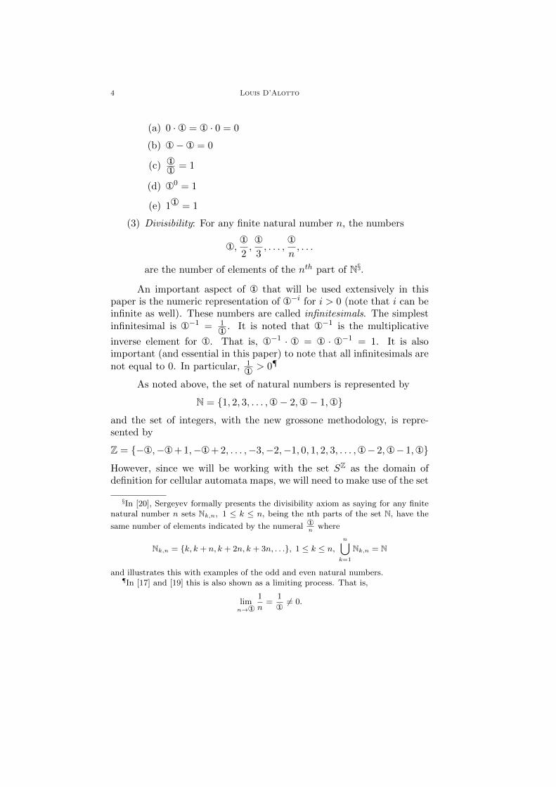
(a) 0 · ① = ① · 0 = 0
(b) ① − ① = 0
(c)①①
= 1
(d) ①0= 1
(e) 1①
= 1
(3) Divisibility: For any finite natural number n, the numbers
①,①
2,①
3, . . . ,
①
n, . . .
are the number of elements of the nthpart of N§
.
An important aspect of ① that will be used extensively in this
paper is the numeric representation of ①−ifor i > 0 (note that i can be
infinite as well). These numbers are called infinitesimals. The simplest
infinitesimal is ①−1=
1
①. It is noted that ①−1
is the multiplicative
inverse element for ①. That is, ①−1 · ① = ① · ①−1= 1. It is also
important (and essential in this paper) to note that all infinitesimals are
not equal to 0. In particular,1
①> 0
¶
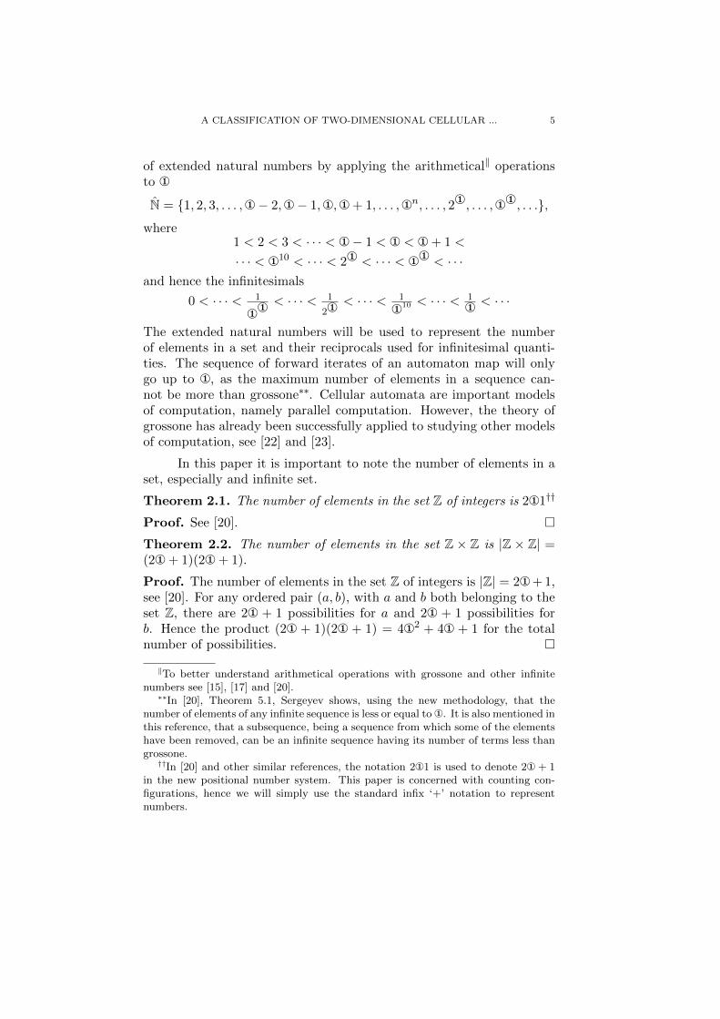
As noted above, the set of natural numbers is represented by
N = {1, 2, 3, . . . ,① − 2,① − 1,①}
and the set of integers, with the new grossone methodology, is repre-
sented by
Z = {−①,−①+1,−①+2, . . . ,−3,−2,−1, 0, 1, 2, 3, . . . ,①− 2,①− 1,①}
However, since we will be working with the set SZas the domain of
definition for cellular automata maps, we will need to make use of the set
§In [20], Sergeyev formally presents the divisibility axiom as saying for any finitenatural number n sets Nk,n, 1 ≤ k ≤ n, being the nth parts of the set N, have the
same number of elements indicated by the numeral ①n where
Nk,n = {k, k + n, k + 2n, k + 3n, . . .}, 1 ≤ k ≤ n,n�
k=1
Nk,n = N
and illustrates this with examples of the odd and even natural numbers.¶In [17] and [19] this is also shown as a limiting process. That is,
limn→①
1n
=1①
�= 0.
A CLASSIFICATION OF TWO-DIMENSIONAL CELLULAR ... 5
of extended natural numbers by applying the arithmetical�operations
to ①
N = {1, 2, 3, . . . ,① − 2,① − 1,①,① + 1, . . . ,①n, . . . , 2①, . . . ,①①, . . .},
where
1 < 2 < 3 < · · · < ① − 1 < ① < ① + 1 <
· · · < ①10 < · · · < 2① < · · · < ①① < · · ·
and hence the infinitesimals
0 < · · · < 1
①①< · · · < 1
2①< · · · < 1
①10 < · · · < 1
①< · · ·
The extended natural numbers will be used to represent the number
of elements in a set and their reciprocals used for infinitesimal quanti-
ties. The sequence of forward iterates of an automaton map will only
go up to ①, as the maximum number of elements in a sequence can-
not be more than grossone∗∗. Cellular automata are important models
of computation, namely parallel computation. However, the theory of
grossone has already been successfully applied to studying other models
of computation, see [22] and [23].
In this paper it is important to note the number of elements in a
set, especially and infinite set.
Theorem 2.1. The number of elements in the set Z of integers is 2①1††
Proof. See [20]. �Theorem 2.2. The number of elements in the set Z × Z is |Z × Z| =(2① + 1)(2① + 1).
Proof. The number of elements in the set Z of integers is |Z| = 2①+1,
see [20]. For any ordered pair (a, b), with a and b both belonging to the
set Z, there are 2① + 1 possibilities for a and 2① + 1 possibilities for
b. Hence the product (2① + 1)(2① + 1) = 4①2+ 4① + 1 for the total
number of possibilities. ��To better understand arithmetical operations with grossone and other infinite
numbers see [15], [17] and [20].∗∗In [20], Theorem 5.1, Sergeyev shows, using the new methodology, that the
number of elements of any infinite sequence is less or equal to ①. It is also mentioned inthis reference, that a subsequence, being a sequence from which some of the elementshave been removed, can be an infinite sequence having its number of terms less thangrossone.
††In [20] and other similar references, the notation 2①1 is used to denote 2① + 1in the new positional number system. This paper is concerned with counting con-figurations, hence we will simply use the standard infix ‘+’ notation to representnumbers.
6 Louis D’Alotto
Theorem 2.3. The number of elements in the set N × Z is |N × Z| =①(2① + 1) = 2①2
+ ①.
Proof. The proof is similar to Theorem 2.2 and hence omitted. �
3. Two-Dimensional Cellular Automata
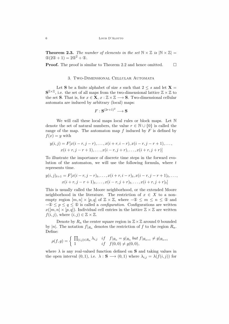
Let S be a finite alphabet of size s such that 2 ≤ s and let X =
SZ×Z, i.e. the set of all maps from the two-dimensional lattice Z× Z to
the set S. That is, for x ∈ X, x : Z×Z −→ S. Two-dimensional cellular
automata are induced by arbitrary (local) maps:
F : S(2r+1)2 −→ S
We will call these local maps local rules or block maps. Let Ndenote the set of natural numbers, the value r ∈ N ∪ {0} is called the
range of the map. The automaton map f induced by F is defined by
f(x) = y with
y(i, j) = F [x(i− r, j − r), . . . , x(i+ r, i− r), x(i− r, j − r + 1), . . . ,
x(i+ r, j − r + 1), . . . , x(i− r, j + r), . . . , x(i+ r, j + r)]
To illustrate the importance of discrete time steps in the forward evo-
lution of the automaton, we will use the following formula, where trepresents time.
y(i, j)t+1 = F [x(i− r, j − r)t, . . . , x(i+ r, i− r)t, x(i− r, j − r + 1)t, . . . ,
x(i+ r, j − r + 1)t, . . . , x(i− r, j + r)t, . . . , x(i+ r, j + r)t]
This is usually called the Moore neighborhood, or the extended Moore
neighborhood in the literature. The restriction of x ∈ X to a non-
empty region [m,n] × [p, q] of Z × Z, where −① ≤ m ≤ n ≤ ① and
−① ≤ p ≤ q ≤ ① is called a configuration. Configurations are written
x([m,n]× [p, q]). Individual cell entries in the lattice Z× Z are written
f(i, j), where (i, j) ∈ Z× Z.Denote by Rn the center square region in Z×Z around 0 bounded
by |n|. The notation f |Rn denotes the restriction of f to the region Rn.
Define:
ρ(f, g) =
� �(i,j)∈Rn
λi,j if f |Rn = g|Rn but f |Rn+1 �= g|Rn+1
1 if f(0, 0) �= g(0, 0),
where λ is any real-valued function defined on S and taking values in
the open interval (0, 1), i.e. λ : S −→ (0, 1) where λi,j = λ(f(i, j)) for
A CLASSIFICATION OF TWO-DIMENSIONAL CELLULAR ... 7
each f(i, j) ∈ S and not infinitesimal, hence each 0 < λi,j < 1. The
metric is defined for f , g ∈ X as follows:
d(f, g) =
�0 if f = gρ(f, g) otherwise
The metric just defined will be called the two-dimensional Kol-mogorov metric and satisfies the nonarchimedean (ultra metric) prop-
erty,
d(x, y) ≤ max{d(x, z), d(z, y)}.
An example of the use of this metric is given in the following example.
Example 3.1. Given the alphabet S = {0, 1}, the following configura-
tion x consisting of all 1’s, and λ(1) = λ(0) = 1/2
(−①,①)����...
.
.
....
.
.
....
.
.
....
.
.
.
(①,①)����...
1 . . . 1 1 1 1 1 . . . 1
1 . . . 1 1 1 1 1 . . . 1
(−①, 0) −→ 1 . . . 1 1 �1� 1 1 . . . 1 ←− (①, 0)1 . . . 1 1 1 1 1 . . . 1
1 . . . 1 1 1 1 1 . . . 1
.
.
.����(−①,−①)
.
.
....
.
.
....
.
.
....
.
.
....����
(①,−①)
The brackets � and � represent the (0, 0) position. Then the con-
figuration below, call it y, is identical to the one above, except for the 0
in the (2, 1) position.
(−①,①)����...
.
.
....
.
.
....
.
.
....
.
.
.
(①,①)����...
1 . . . 1 1 1 1 1 . . . 1
1 . . . 1 1 1 1 0 . . . 1
(−①, 0) −→ 1 . . . 1 1 �1� 1 1 . . . 1 ←− (①, 0)1 . . . 1 1 1 1 1 . . . 1
1 . . . 1 1 1 1 1 . . . 1
.
.
.����(−①,−①)
.
.
....
.
.
....
.
.
....
.
.
....����
(①,−①)
8 Louis D’Alotto
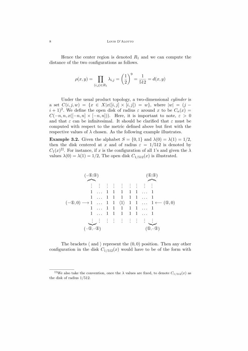
Hence the center region is denoted R1 and we can compute the
distance of the two configurations as follows.
ρ(x, y) =�
(i,j)∈R1
λi,j =
�1
2
�9
=1
512= d(x, y)
Under the usual product topology, a two-dimensional cylinder is
a set C(i, j, w) = {x ∈ X|x([i, j] × [i, j]) = w}, where |w| = (j −i + 1)
2. We define the open disk of radius ε around x to be Cn(x) =
C(−n, n, x([−n, n] × [−n, n])). Here, it is important to note, ε > 0
and that ε can be infinitesimal. It should be clarified that ε must be
computed with respect to the metric defined above but first with the
respective values of λ chosen. As the following example illustrates.
Example 3.2. Given the alphabet S = {0, 1} and λ(0) = λ(1) = 1/2,then the disk centered at x and of radius ε = 1/512 is denoted by
C1(x)‡‡. For instance, if x is the configuration of all 1’s and given the λ
values λ(0) = λ(1) = 1/2, The open disk C1/512(x) is illustrated.
(−①,①)����...
.
.
....
.
.
....
.
.
....
.
.
.
(①,①)����...
1 . . . 1 1 1 1 1 . . . 1
1 . . . 1 1 1 1 1 . . . 1
(−①, 0) −→ 1 . . . 1 1 �1� 1 1 . . . 1 ←− (①, 0)1 . . . 1 1 1 1 1 . . . 1
1 . . . 1 1 1 1 1 . . . 1
.
.
.����(−①,−①)
.
.
....
.
.
....
.
.
....
.
.
....����
(①,−①)
The brackets � and � represent the (0, 0) position. Then any other
configuration in the disk C1/512(x) would have to be of the form with
‡‡We also take the convention, once the λ values are fixed, to denote C1/512(x) asthe disk of radius 1/512.
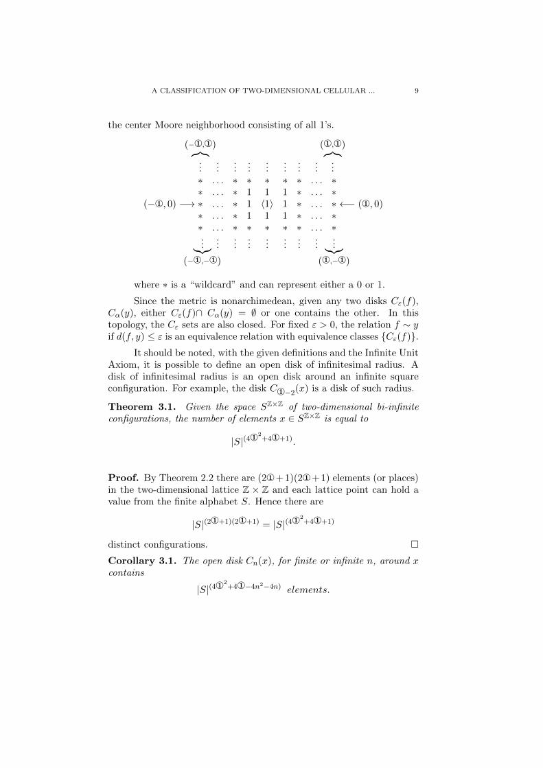
A CLASSIFICATION OF TWO-DIMENSIONAL CELLULAR ... 9
the center Moore neighborhood consisting of all 1’s.
(−①,①)����...
.
.
....
.
.
....
.
.
....
.
.
.
(①,①)����...
∗ . . . ∗ ∗ ∗ ∗ ∗ . . . ∗∗ . . . ∗ 1 1 1 ∗ . . . ∗
(−①, 0) −→ ∗ . . . ∗ 1 �1� 1 ∗ . . . ∗ ←− (①, 0)∗ . . . ∗ 1 1 1 ∗ . . . ∗∗ . . . ∗ ∗ ∗ ∗ ∗ . . . ∗...����
(−①,−①)
.
.
....
.
.
....
.
.
....
.
.
....����
(①,−①)
where ∗ is a “wildcard” and can represent either a 0 or 1.
Since the metric is nonarchimedean, given any two disks Cε(f),Cα(y), either Cε(f)∩ Cα(y) = ∅ or one contains the other. In this
topology, the Cε sets are also closed. For fixed ε > 0, the relation f ∼ yif d(f, y) ≤ ε is an equivalence relation with equivalence classes {Cε(f)}.
It should be noted, with the given definitions and the Infinite Unit
Axiom, it is possible to define an open disk of infinitesimal radius. A
disk of infinitesimal radius is an open disk around an infinite square
configuration. For example, the disk C①−2(x) is a disk of such radius.
Theorem 3.1. Given the space SZ×Z of two-dimensional bi-infiniteconfigurations, the number of elements x ∈ SZ×Z is equal to
|S|(4①2+4①+1).
Proof. By Theorem 2.2 there are (2①+1)(2①+1) elements (or places)
in the two-dimensional lattice Z × Z and each lattice point can hold a
value from the finite alphabet S. Hence there are
|S|(2①+1)(2①+1)= |S|(4①
2+4①+1)
distinct configurations. �Corollary 3.1. The open disk Cn(x), for finite or infinite n, around xcontains
|S|(4①2+4①−4n2−4n) elements.
10 Louis D’Alotto
Proof. An open disk Cn(x) around x must have a fixed square center
where a side equals 2n+ 1. The number of possible configurations out-
side this square center must be computed. Above the square there are
|S|(2①+1)(①−n)possible configurations. Below the square, the same. To
the right of the square, there are |S|(2n+1)(①−n)possible configurations
and the same to the left of the center square. Hence the total number of
possible configurations (elements in the open disk Cn(x)) are given by
the following computation.
|S|(2①+1)(①−n) · |S|(2①+1)(①−n) · |S|(2n+1)(①−n) · |S|(2n+1)(①−n)
= |S|2(2①+1)(①−n) · |S|2(2n+1)(①−n)
= |S|(4①2+4①−4n2−4n)
�Example 3.3. For n = ①− 1, C①−1
(x) is a disk of infinitesimal radius
and contains
|S|(4①2+4①−4(①−1)2−4(①−1)
= |S|8①
points.
As is seen, disks of infinitesimal radius contain, although still in-
finite, many fewer points than disks of finite radius. This is in contrast
to the one-dimensional case§§
where there can be finitely many elements
in a disk of infinitesimal radius.
To understand the dynamics of cellular automata it is necessary
to study the forward iterates of configurations that equal or match those
of a given configuration, call it “x”, on a given interval of Z. Here the
relation x ∼ y iff ∀i ∈ N0, (f i(y))([m,n] × [p, q]) = (f i
(x))([m,n] ×[p, q]) forms an equivalence relation with equivalence classes denoted by
Bm,n,p,q(x). That is,
Bm,n,p,q(x) = {y | (f i(y))([m,n]× [p, q]) = (f i
(x))([m,n]× [p, q]) ∀i ∈ N0}.
Bm,n,p,q(x) is the set of y for which (f i(y))([m,n]×[p, q]) = (f i
(x))([m,n]× [p, q]), for m ≤ 0 ≤ n and p ≤ 0 ≤ q, under forward iterations of the
cellular automaton function. That is, ∀i ∈ N0. Recall, (f i(y))([m,n] ×
[p, q]) represents configurations and that the cellular automaton func-
tion, f is first applied to the entire configuration x (or y), and then
restricted to the region [m,n] × [p, q]. Note that m and/or p can equal
−① + k and n and/or q can equal ① − k, for some finite integer k ≥0. In those cases the configurations are left-sided, right-sided or both
§§ See [5] for the one-dimensional analysis and classification of cellular automatausing grossone.
A CLASSIFICATION OF TWO-DIMENSIONAL CELLULAR ... 11
sided infinite. Hence elements in the Bm,n,p,q(x) classes will agree with
x([m,n]× [p, q]) and all forward iterations of x([m,n]× [p, q]) under theautomaton map f . This will form the effect of an infinite vertical rect-
angular prism, not necessarily symmetric, around the central window.
The dynamical analysis of cellular automata presented herein is
based on counting the number of elements in the entire domain space,
X. Hence, in this section we will use ① to count the number of ele-
ments in the class Bm,n,p,q(x) whose forward iterates match those of xin some window containing the center and develop a simple classification
of two-dimensional cellular automata based on this count. Similar to the
one-dimensional case, two-dimensional cellular automata rules are thus
partitioned into three classes.
Definition 3.1. Define the classes of two-dimensional cellular au-
tomata, f , as follows:
(1) f ∈ A if there is a Bm,n,p,q(x) that contains at least |S|4(①2+①)−k
elements, for some finite integer k ≥ 0.
(2) f ∈ B if there is a Bm,n,p,q(x) that contains at least |S|α①2+β①−k
elements, for some finite integer k ≥ 0, 0 < α < 4 and not
infinitesimal, and β a finite non-infinitesimal real number, but fdoes not belong to class A.
(3) f ∈ C otherwise.
Class C is the most chaotic class of automata. Indeed, in this class
there may only be finitely many elements or simple infinitely many
elements in any Bm,n(x) class. Hence, beginning with an initial con-
figuration, most other configurations will diverge away from the ini-
tial configuration. Automata in class A are the least chaotic and most
elements will equal an initial configuration upon repeated applications
(iterations) of the automata rule on the infinite strip. The following
theorem shows the relationship between an open disk and the number
of configurations in a Bm,n,p,q(x) class.
Theorem 3.2. If there exists a Bm,n,p,q(x), for cellular automaton f ,that contains an open disk of non-infinitesimal radius, then f ∈ A.
Proof. If there is a Bm,n,p,q(x), for cellular automaton f that contains
an open disk Cn(x) of non-infinitesimal radius, then Cn(x) contains
|S|(4①2+4①−4n2−4n)
elements. Therefore Bm,n,p,q(x) contains at least
|S|(4①2+4①−4n2−4n)
elements. Since n is finite, take finite k = 4n2 − 4nand by Definition 3.1 the theorem is proved. �
12 Louis D’Alotto
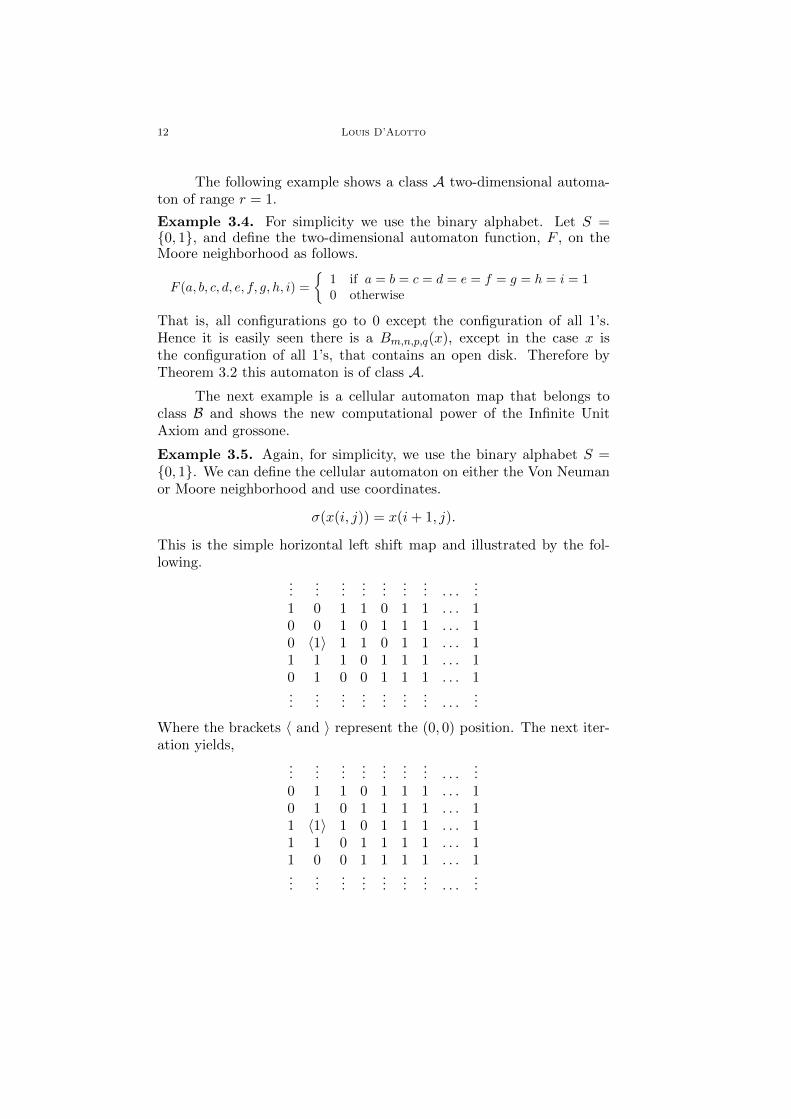
The following example shows a class A two-dimensional automa-
ton of range r = 1.
Example 3.4. For simplicity we use the binary alphabet. Let S =
{0, 1}, and define the two-dimensional automaton function, F , on the
Moore neighborhood as follows.
F (a, b, c, d, e, f, g, h, i) =
�1 if a = b = c = d = e = f = g = h = i = 1
0 otherwise
That is, all configurations go to 0 except the configuration of all 1’s.
Hence it is easily seen there is a Bm,n,p,q(x), except in the case x is
the configuration of all 1’s, that contains an open disk. Therefore by
Theorem 3.2 this automaton is of class A.
The next example is a cellular automaton map that belongs to
class B and shows the new computational power of the Infinite Unit
Axiom and grossone.
Example 3.5. Again, for simplicity, we use the binary alphabet S =
{0, 1}. We can define the cellular automaton on either the Von Neuman
or Moore neighborhood and use coordinates.
σ(x(i, j)) = x(i+ 1, j).
This is the simple horizontal left shift map and illustrated by the fol-
lowing.
.
.
....
.
.
....
.
.
....
.
.
. . . ....
1 0 1 1 0 1 1 . . . 1
0 0 1 0 1 1 1 . . . 1
0 �1� 1 1 0 1 1 . . . 1
1 1 1 0 1 1 1 . . . 1
0 1 0 0 1 1 1 . . . 1
.
.
....
.
.
....
.
.
....
.
.
. . . ....
Where the brackets � and � represent the (0, 0) position. The next iter-
ation yields,
.
.
....
.
.
....
.
.
....
.
.
. . . ....
0 1 1 0 1 1 1 . . . 1
0 1 0 1 1 1 1 . . . 1
1 �1� 1 0 1 1 1 . . . 1
1 1 0 1 1 1 1 . . . 1
1 0 0 1 1 1 1 . . . 1
.
.
....
.
.
....
.
.
....
.
.
. . . ....
A CLASSIFICATION OF TWO-DIMENSIONAL CELLULAR ... 13
Therefore any other configuration, y, in Bm,n,p,q(x) would have to
agree at least on the right of the center square, the (0, 0) position, out
to ①. Hence there are at most
|S|①(2①+1) · |S|①(2①+1) · |S|① = |S|4①2+3①
configurations and clearly by Definition 3.1 the left shift, σ(x(i, j)) =
x(i+ 1, j), belongs in B.
4. Discussion and Conclusion
In this paper a classification scheme for two-dimensional cellular
automata, based on the Infinite unit axion and grossone, has been pre-
sented. The entire domain space of two-dimensional automata, X =
SZ×Z, contains |S|(2①+1)(2①+1)
configurations. This puts an upper
bound representation on the number of elements in the entire space,
hence we sub-divided the space into three components and used this to
build a classification on the number of configurations whose forward evo-
lution, under a cellular automaton, equal those (on a central window)
of a given initial configuration.
This classification is based on a numeric representation of count-
ing elements in a set. Automata in class A are the least chaotic, having
a very large number of configurations equaling those of a given con-
figuration, on some central window¶¶, upon forward iterations of the
automaton map. Automata in class B, such as the left shift automaton,
are more chaotic than those in class A. However, it seems that they can
still be described without too much complexity. Automata in class Care more difficult to find and are the most chaotic in the respect that
there are relatively very few other configurations that will follow and
stay close to a given. Indeed, the number of configurations that equal
a given initial configuration, upon forward iterations, is much less than
the other classes and may be simple infinite (either ①, or ①2, . . . , or ①n,
or some part thereof), finite or a single configuration. Conway’s Game
of Life has been shown to be capable of universal computation. Due to
the nature of universal computation, some of these automata can fall
into class C. It is left as an open problem to prove or disprove this. It
is noted that the presented classification would be stronger if there was
an algorithm to determine membership in the different classes and it is
also posed as an open problem.
¶¶Given the definition of the metric, it is allowable to say “staying close together”upon forward iterations.
14 Louis D’Alotto
References
[1] E. R. Berlekamp, J. H. Conway and R. K. Guy, Winning Ways for YourMathematical Plays, Volume 4, 2nd Edition, A. K. Peters, Wellesley, Mas-sachusettes, 2004.
[2] C. R. Calidonna, A. Naddeo, G. A. Trunfio and S. Di Gregorio, Fromclassical infinite space-time CA to a hybrid CA model for natural sciences mod-eling, Applied Mathematics and Computation, 218(16)(2012), 8137-8150.
[3] B. Chopard and M. Droz, Cellular Automata Modeling of Physical Systems,Cambridge University Press, 1998.
[4] L. D’Alotto, Cellular automata using infinite computations, Applied Mathe-matics and Computation, 218(16)(2012), 8077-8082.
[5] L. D’Alotto, A classification of one-dimensional cellular automata us-ing infinite computations, Applied Mathematics and Computation (2014),http://dx.doi.org/10.1016/j.amc.2014.06.087
[6] D. D’Ambrosio, G. Filippone, D. Marocco, R. Rongo and W. Spataro,Efficient application of GPGPU for lava flow hazard mapping, The Journal ofSupercomputing, 65(2)(2013), 630-644.
[7] S. De Cosmis and R. De Leone, The use of grossone in mathematical pro-gramming and operations research, Applied Mathematics and Computation,218(16)(2012), 8029-8038.
[8] R. Gilman, Classes of linear automata, Ergodic Theory and Dynamical Systems,7(1987), 105-118.
[9] G. A. Hedlund, Edomorphisms and automorphisms of the shift dynamical sys-tem, Math. Sys. Theory 3(1969), 51-59.
[10] D. I. Iudin, Ya. D. Sergeyev and M. Hayakawa, Interpretation of percola-tion in terms of infinity computations, Applied Mathematics and Computation,218(16)(2012), 8099-8111.
[11] G. Lolli, Infinitesimals and infinities in the history of mathematics: A briefsurvey, Applied Mathematics and Computation, 218(16)(2012), 7979-7988.
[12] G. Lolli, Metamathematical investigations on the theory of grossone, Preprint,submitted and accepted for publication in Applied Mathematics and Computa-tion, Elsevier.
[13] M. Margenstern, Using grossone to count the number of elements of infinitesets and the connection with bijections, p-adic numbers, Ultrametric Analysisand Applications, 3(3)(2011), 196-204.
[14] M. Margenstern, An application of grossone to the study of a family of tilingsof the hyperbolic plane, Applied Mathematics and Computation, 218(16)(2012),8005-8018.
[15] F. Montagna, G. Simi and A. Sorbi, Taking the Piraha seriously, CommunNonlinear Science and Numerical Simulation, 21(2015), 52-69.
[16] L. Narici, E. Beckenstein and G. Bachman, Functional Analysis and Valu-ation Theory, Marcel Dekker, Inc., NY, 1971.
[17] Ya. D. Sergeyev, Arithmetic of Infinity, Edizioni Orizzonti Meridionali, Italy,2003.
[18] Ya. D. Sergeyev, Numerical point of view on calculus for functions assum-ing finite, Infinite, and Infinitesimal Values Over Finite, Infinite, and Infinites-imal Domains, Nonlinear Analysis Series A: Theory, Methods & Applications,71(12)(2009), e1688-e1707.
A CLASSIFICATION OF TWO-DIMENSIONAL CELLULAR ... 15
[19] Ya. D. Sergeyev, Numerical Computations with Infinite and InfinitesimalNumbers: Theory and Applications, Dynamics of Information Systems: Algo-rithmic Approaches edited by Sorokin, A., Pardalos, P. M., Springer, New York,1 - 66, 2013.
[20] Ya. D. Sergeyev, A new applied approach for executing computations withinfinite and infinitesimal quantities, Informatica, 19(4)(2008), 567-596.
[21] Ya. D. Sergeyev, Measuring fractals by infinite and infinitesimal numbers,Mathematical Methods, Physical Methods & Simulation Science and Technology,1(1)(2008), 217-237.
[22] Ya. D. Sergeyev and A. Garro, Observability of turing machines: A refine-ment of the theory of computation, Informatica, 21(3)(2010), 425-454.
[23] Ya. D. Sergeyev and A. Garro, Single-tape and multi-tape turing machinesthrough the lens of grossone methodology, The Journal of Supercomputing,65(2)(2013), 645-663.
[24] G. Ch. Sirakoulis, I. Krafyllidis and W. Spataro, A computational in-telligent oxidation process model and its VLSI implementation, InternationalConference on Scientific Computing Proceedings, (2009), 329-335.
[25] G. A. Trunfio, Predicting wildfire spreading through a hexagonal cellular au-tomata model, In: P.M.A. Sloot, B. Chopard, and A.G. Hoekstra, Editors, ACRI2004, LNCS 3305, Spring, Berlin, (2004), 725-734.
[26] G. A. Trunfio, D. D’Ambrosio, R. Rongo, W. Spataro and S. Di Grego-
rio, A new algorithm for simulating wilfire spread through cellular automata,ACM Transactions on Modeling and Computer Simulation, 22(2011), 1-26.
[27] S. Wolfram, Statistical mechanics of cellular automata, Reviews of ModernPhysics, 55(3)(1983), 601-644.
[28] S. Wolfram, A New Kind of Science, Wolfram Media, Inc., IL, 2002.[29] S. Wolfram, Universality and complexity in cellular automata, Physica D,
10(1984), 1-35.[30] A. Zhigljavsky, Computing sums of conditionally convergent and divergent
series using the concept of grossone, Applied Mathematics and Computation,218(16)(2012), 8064-8076.