Embed Size (px)
Citation preview
'
&
$
%
Large-MIMO: A Technology Whose Time Has Come
A. Chockalingam and B. Sundar Rajan
(achockal,[email protected])
April 2010
Department of Electrical Communication Engineering
(http://www.ece.iisc.ernet.in/)
Indian Institute of Science
Bangalore – 560 012. INDIA
A. Chockalingam and B. Sundar Rajan: Large-MIMO: A Technology Whose Time Has Come Dept. of ECE, IISc, Bangalore, April 2010 1'
&
$
%
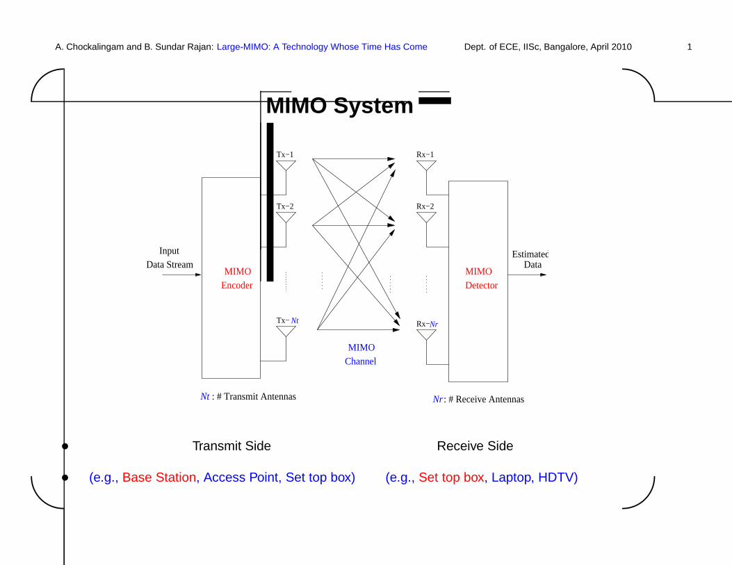
MIMO System
Detector
EstimatedData
MIMO Channel
Input Data Stream
Encoder
Tx−1
Tx−2
Tx− Rx−
Rx−2
Rx−1
MIMOMIMO
NrNt
Nt Nr : # Transmit Antennas : # Receive Antennas
• Transmit Side Receive Side
• (e.g., Base Station, Access Point, Set top box) (e.g., Set top box, Laptop, HDTV)
A. Chockalingam and B. Sundar Rajan: Large-MIMO: A Technology Whose Time Has Come Dept. of ECE, IISc, Bangalore, April 2010 2'
&
$
%
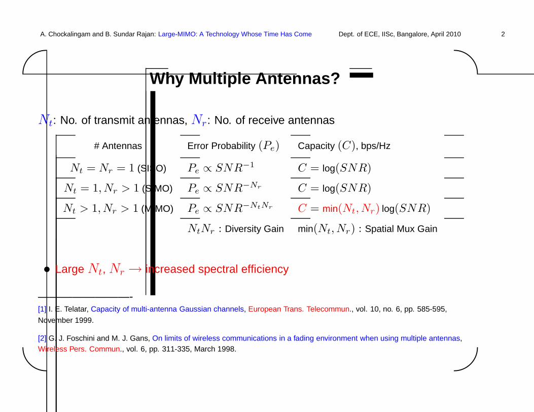
Why Multiple Antennas?
Nt: No. of transmit antennas, Nr: No. of receive antennas
# Antennas Error Probability (Pe) Capacity (C), bps/Hz
Nt = Nr = 1 (SISO) Pe ∝ SNR−1 C = log(SNR)
Nt = 1, Nr > 1 (SIMO) Pe ∝ SNR−Nr C = log(SNR)
Nt > 1, Nr > 1 (MIMO) Pe ∝ SNR−NtNr C = min(Nt, Nr) log(SNR)
NtNr : Diversity Gain min(Nt, Nr) : Spatial Mux Gain
• Large Nt, Nr → increased spectral efficiency
————————-[1] I. E. Telatar, Capacity of multi-antenna Gaussian channels, European Trans. Telecommun., vol. 10, no. 6, pp. 585-595,
November 1999.
[2] G. J. Foschini and M. J. Gans, On limits of wireless communications in a fading environment when using multiple antennas,Wireless Pers. Commun., vol. 6, pp. 311-335, March 1998.
A. Chockalingam and B. Sundar Rajan: Large-MIMO: A Technology Whose Time Has Come Dept. of ECE, IISc, Bangalore, April 2010 3'
&
$
%
Large-MIMO Approach
• Employ large number (several tens) of antennas at the Tx and Rx
• Achieve high spectral efficiencies (tens to hundreds of bps/Hz)
– Data rate (bps) = Spectral efficiency (bps/Hz) × Bandwidth (Hz)
– e.g., 100 bps/Hz =⇒ 1 Gbps rate in just 10 MHz bandwidth
• Limitation in current MIMO standards
– spectral efficiency: ∼ 10 bps/Hz only
– 2 to 4 transmit antennas
– e.g., 750 Mbps in 80 MHz in 802.11n using 4 Tx antennas
– do not exploit the potential of large spatial dimensions
A. Chockalingam and B. Sundar Rajan: Large-MIMO: A Technology Whose Time Has Come Dept. of ECE, IISc, Bangalore, April 2010 4'
&
$
%
Technological Challenges in Realizing Large-MIMO
• Placement of large number of antennas in communicationterminals
– Feasible in moderately sized communication terminals (e.g., Set top boxes,
Laptops, BS towers)
– use high carrier frequencies for small carrier wavelengths (e.g., 5 GHz, 60 GHz)
• RF technologies
– Multiple IF/RF transmit and receive chains
• Large-MIMO detection
– Need low-complexity detectors
• Channel estimation
– Estimation of large number of channel coefficients
A. Chockalingam and B. Sundar Rajan: Large-MIMO: A Technology Whose Time Has Come Dept. of ECE, IISc, Bangalore, April 2010 5'
&
$
%
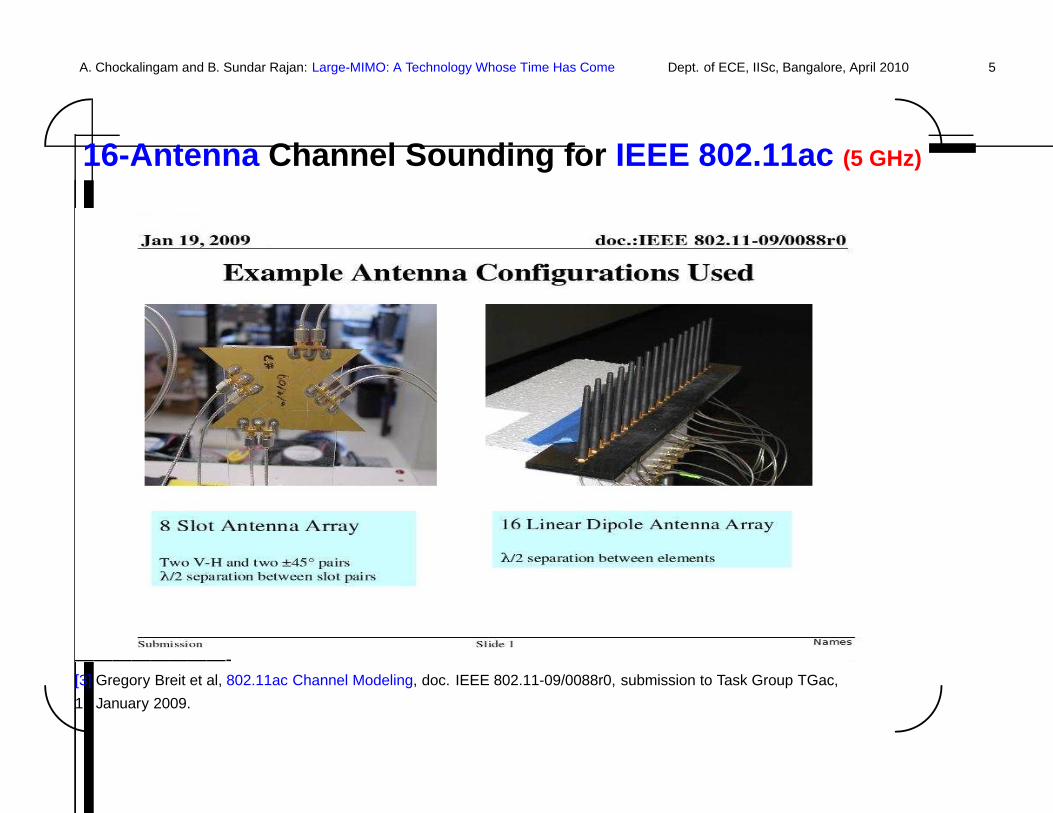
16-Antenna Channel Sounding for IEEE 802.11ac (5 GHz)
————————-[3] Gregory Breit et al, 802.11ac Channel Modeling, doc. IEEE 802.11-09/0088r0, submission to Task Group TGac,
19 January 2009.
A. Chockalingam and B. Sundar Rajan: Large-MIMO: A Technology Whose Time Has Come Dept. of ECE, IISc, Bangalore, April 2010 6'
&
$
%
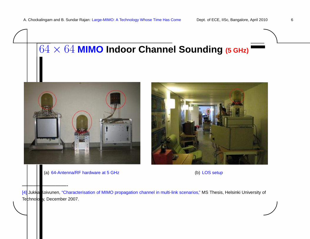
64 × 64 MIMO Indoor Channel Sounding (5 GHz)
(a) 64-Antenna/RF hardware at 5 GHz (b) LOS setup
————————-[4] Jukka Koivunen, “Characterisation of MIMO propagation channel in multi-link scenarios,” MS Thesis, Helsinki University of
Technology, December 2007.
A. Chockalingam and B. Sundar Rajan: Large-MIMO: A Technology Whose Time Has Come Dept. of ECE, IISc, Bangalore, April 2010 7'
&
$
%
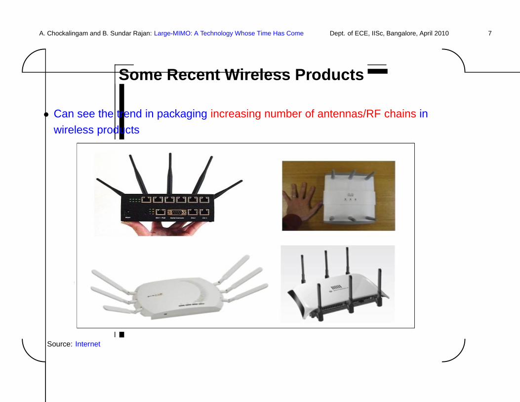
Some Recent Wireless Products
• Can see the trend in packaging increasing number of antennas/RF chains in
wireless products
Source: Internet
A. Chockalingam and B. Sundar Rajan: Large-MIMO: A Technology Whose Time Has Come Dept. of ECE, IISc, Bangalore, April 2010 8'
&
$
%
Detection Complexity: A Key Challenge in Large-MIMO
• Optimal detection has exponential complexity in # transmit
antennas
• Need low-complexity algorithms that are near-optimal
• A possible approach to low-complexity solutions
– Seek algorithms from machine learning (ML)
– Large-dimension problems are routinely addressed in other
areas (e.g., computer vision, web search) using ML algorithms
– Communications area too has benefited from ML algorithms
∗ MUD in CDMA (large # users), Turbo/LDPC decoding (large frame sizes)
A. Chockalingam and B. Sundar Rajan: Large-MIMO: A Technology Whose Time Has Come Dept. of ECE, IISc, Bangalore, April 2010 9'
&
$
%
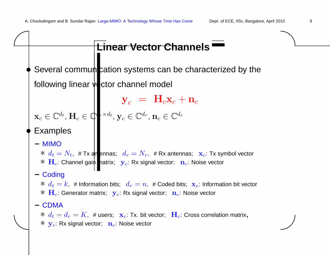
Linear Vector Channels
• Several communication systems can be characterized by the
following linear vector channel model
yc = Hcxc + nc
xc ∈ Cdt , Hc ∈ Cdr×dt , yc ∈ Cdr , nc ∈ Cdr
• Examples
– MIMO∗ dt = Nt, # Tx antennas; dr = Nr , # Rx antennas; xc: Tx symbol vector
∗ Hc: Channel gain matrix; yc: Rx signal vector; nc: Noise vector
– Coding∗ dt = k, # Information bits; dr = n, # Coded bits; xc: Information bit vector
∗ Hc: Generator matrix; yc: Rx signal vector; nc: Noise vector
– CDMA∗ dt = dr = K , # users; xc: Tx. bit vector; Hc: Cross correlation matrix,∗ yc: Rx signal vector; nc: Noise vector
A. Chockalingam and B. Sundar Rajan: Large-MIMO: A Technology Whose Time Has Come Dept. of ECE, IISc, Bangalore, April 2010 10'
&
$
%
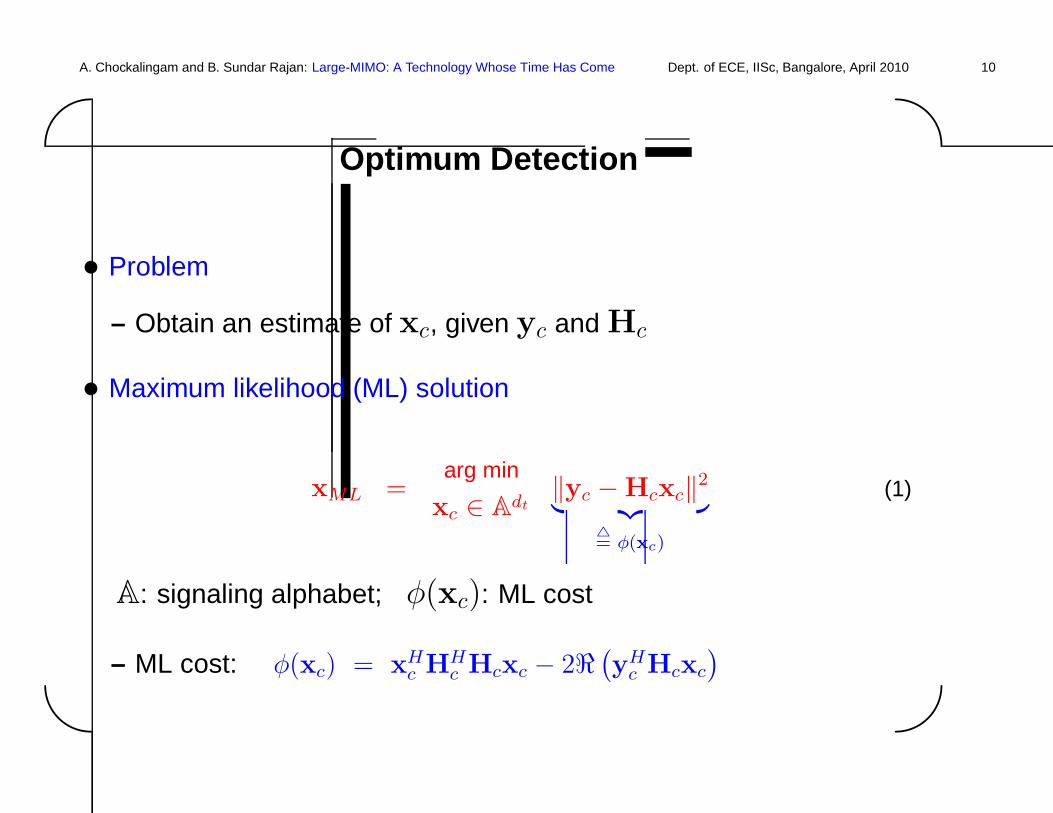
Optimum Detection
• Problem
– Obtain an estimate of xc, given yc and Hc
• Maximum likelihood (ML) solution
xML =arg min
xc ∈ Adt‖yc − Hcxc‖2
︸ ︷︷ ︸△= φ(xc)
(1)
A: signaling alphabet; φ(xc): ML cost
– ML cost: φ(xc) = xHc HH
c Hcxc − 2ℜ(yH
c Hcxc
)
A. Chockalingam and B. Sundar Rajan: Large-MIMO: A Technology Whose Time Has Come Dept. of ECE, IISc, Bangalore, April 2010 11'
&
$
%
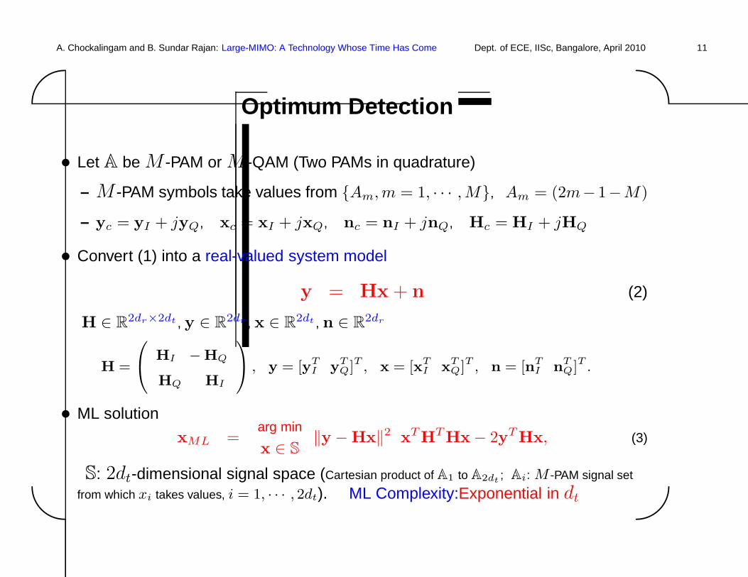
Optimum Detection
• Let A be M -PAM or M -QAM (Two PAMs in quadrature)
– M -PAM symbols take values from {Am, m = 1, · · · , M}, Am = (2m− 1−M)
– yc = yI + jyQ, xc = xI + jxQ, nc = nI + jnQ, Hc = HI + jHQ
• Convert (1) into a real-valued system model
y = Hx + n (2)
H ∈ R2dr×2dt , y ∈ R
2dr , x ∈ R2dt , n ∈ R
2dr
H =
0
@
HI −HQ
HQ HI
1
A , y = [yTI y
TQ]T , x = [xT
I xTQ]T , n = [nT
I nTQ]T .
• ML solution
xML =arg min
x ∈ S‖y − Hx‖2 xT HT Hx − 2yT Hx, (3)
S: 2dt-dimensional signal space (Cartesian product of A1 to A2dt ; Ai: M -PAM signal set
from which xi takes values, i = 1, · · · , 2dt). ML Complexity:Exponential in dt
A. Chockalingam and B. Sundar Rajan: Large-MIMO: A Technology Whose Time Has Come Dept. of ECE, IISc, Bangalore, April 2010 12'
&
$
%
Optimum Detection
• Maximum a posteriori (MAP) solution
– Consider square M -QAM
– Each entry of x belongs to a√
M -PAM constellation
– Let b(0)i , b
(1)i , · · · , b
(q−1)i denote the q = log2(
√M) constituent bits of xi
– xi can be written as
xi =
q−1∑
j=0
2j b(j)i , i = 0, 1, · · · , 2dt − 1
– Let the bit vector b ∈ {±1}2qdt be written as
b△=
[b(0)0 · · · b(q−1)
0 b(0)1 · · · b(q−1)
1 · · · b(0)2dt−1 · · · b
(q−1)2dt−1
]T
– Defining c△= [20 21 · · · 2q−1], x can be written as
x = (I2dt⊗ c)b
A. Chockalingam and B. Sundar Rajan: Large-MIMO: A Technology Whose Time Has Come Dept. of ECE, IISc, Bangalore, April 2010 13'
&
$
%
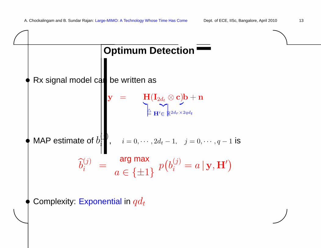
Optimum Detection
• Rx signal model can be written as
y = H(I2dt⊗ c)︸ ︷︷ ︸
△= H′∈ R2dr×2qdt
b + n
• MAP estimate of b(j)i , i = 0, · · · , 2dt − 1, j = 0, · · · , q − 1 is
b(j)i =
arg max
a ∈ {±1} p(b(j)i = a |y,H′)
• Complexity: Exponential in qdt
A. Chockalingam and B. Sundar Rajan: Large-MIMO: A Technology Whose Time Has Come Dept. of ECE, IISc, Bangalore, April 2010 14'
&
$
%
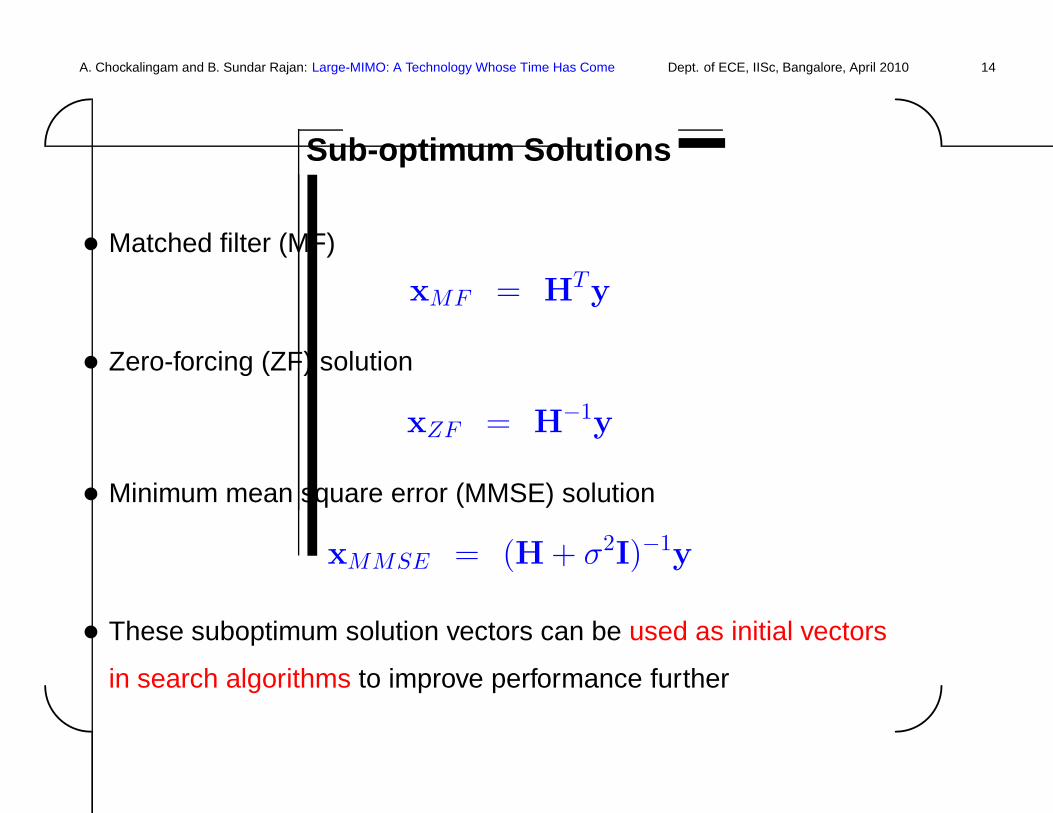
Sub-optimum Solutions
• Matched filter (MF)
xMF = HTy
• Zero-forcing (ZF) solution
xZF = H−1y
• Minimum mean square error (MMSE) solution
xMMSE = (H + σ2I)−1y
• These suboptimum solution vectors can be used as initial vectors
in search algorithms to improve performance further
A. Chockalingam and B. Sundar Rajan: Large-MIMO: A Technology Whose Time Has Come Dept. of ECE, IISc, Bangalore, April 2010 15'
&
$
%
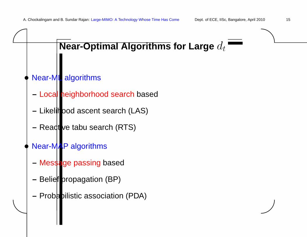
Near-Optimal Algorithms for Large dt
• Near-ML algorithms
– Local neighborhood search based
– Likelihood ascent search (LAS)
– Reactive tabu search (RTS)
• Near-MAP algorithms
– Message passing based
– Belief propagation (BP)
– Probabilistic association (PDA)
A. Chockalingam and B. Sundar Rajan: Large-MIMO: A Technology Whose Time Has Come Dept. of ECE, IISc, Bangalore, April 2010 16'
&
$
%
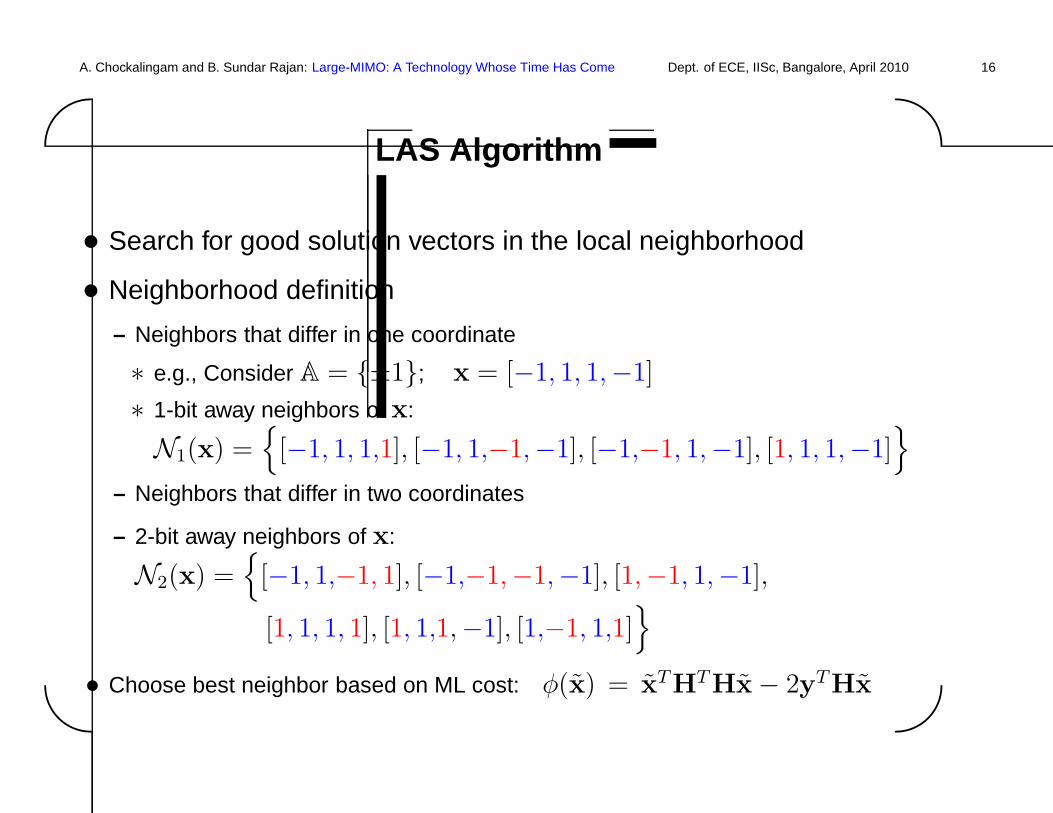
LAS Algorithm
• Search for good solution vectors in the local neighborhood
• Neighborhood definition
– Neighbors that differ in one coordinate
∗ e.g., Consider A = {±1}; x = [−1, 1, 1,−1]
∗ 1-bit away neighbors of x:
N1(x) ={
[−1, 1, 1,1], [−1, 1,−1,−1], [−1,−1, 1,−1], [1, 1, 1,−1]}
– Neighbors that differ in two coordinates
– 2-bit away neighbors of x:
N2(x) ={
[−1, 1,−1, 1], [−1,−1,−1,−1], [1,−1, 1,−1],
[1, 1, 1, 1], [1, 1,1,−1], [1,−1, 1,1]}
• Choose best neighbor based on ML cost: φ(x) = xTHTHx − 2yTHx
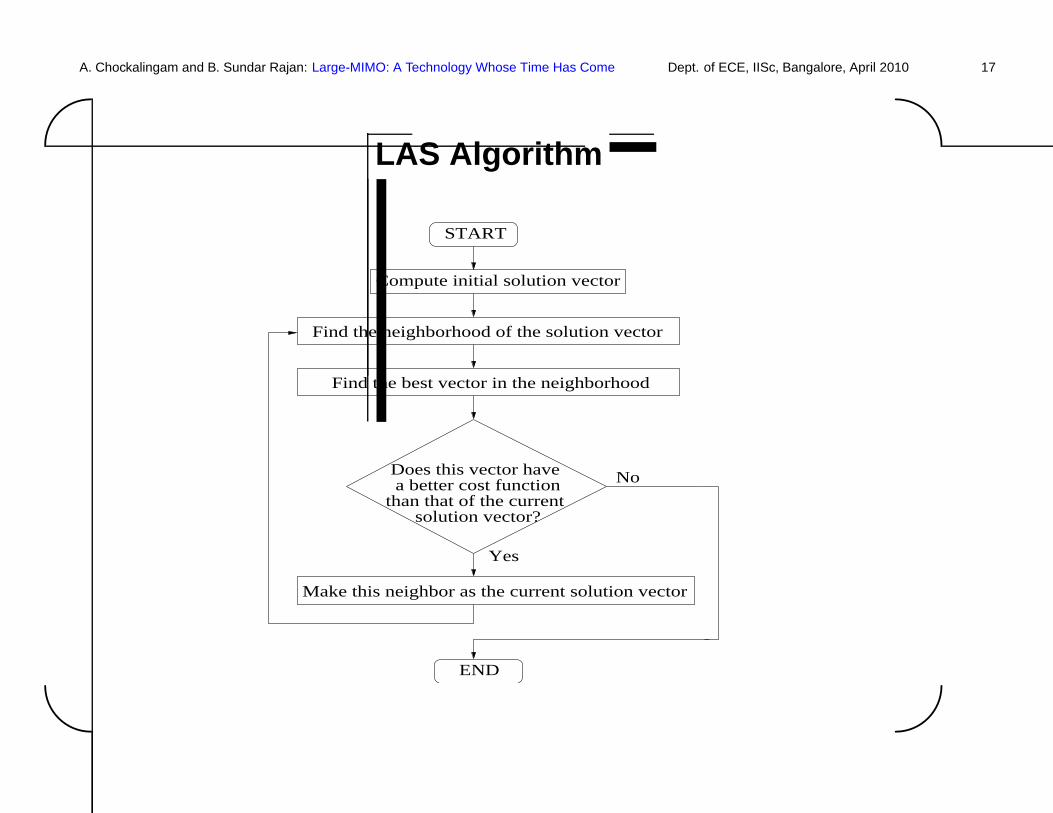
A. Chockalingam and B. Sundar Rajan: Large-MIMO: A Technology Whose Time Has Come Dept. of ECE, IISc, Bangalore, April 2010 17'
&
$
%
LAS Algorithm
END
START
Yes
No
than that of the currenta better cost functionDoes this vector have
solution vector?
Compute initial solution vector
Find the neighborhood of the solution vector
Find the best vector in the neighborhood
Make this neighbor as the current solution vector
A. Chockalingam and B. Sundar Rajan: Large-MIMO: A Technology Whose Time Has Come Dept. of ECE, IISc, Bangalore, April 2010 18'
&
$
%
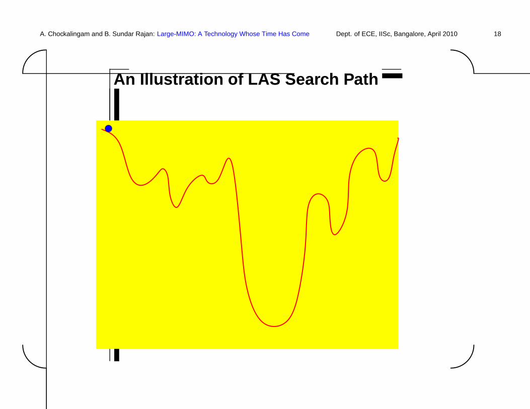
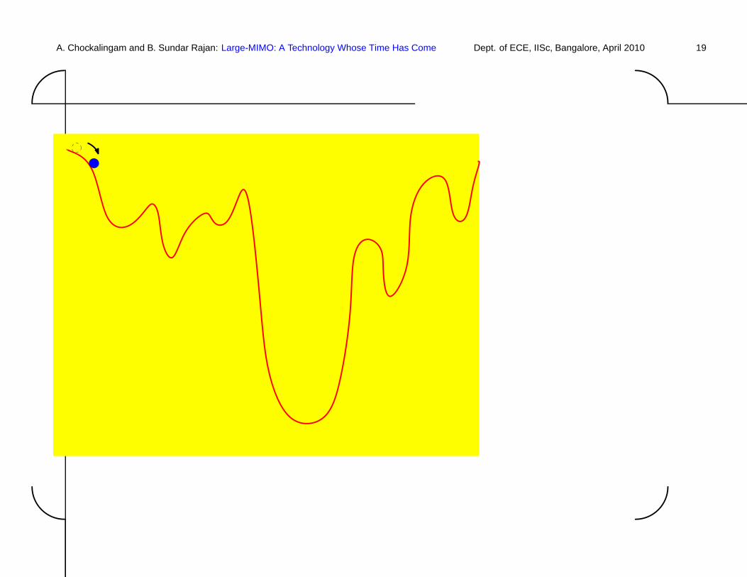
An Illustration of LAS Search Path
A. Chockalingam and B. Sundar Rajan: Large-MIMO: A Technology Whose Time Has Come Dept. of ECE, IISc, Bangalore, April 2010 19'
&
$
%

A. Chockalingam and B. Sundar Rajan: Large-MIMO: A Technology Whose Time Has Come Dept. of ECE, IISc, Bangalore, April 2010 20'
&
$
%

A. Chockalingam and B. Sundar Rajan: Large-MIMO: A Technology Whose Time Has Come Dept. of ECE, IISc, Bangalore, April 2010 21'
&
$
%

A. Chockalingam and B. Sundar Rajan: Large-MIMO: A Technology Whose Time Has Come Dept. of ECE, IISc, Bangalore, April 2010 22'
&
$
%
Local minima trap
A. Chockalingam and B. Sundar Rajan: Large-MIMO: A Technology Whose Time Has Come Dept. of ECE, IISc, Bangalore, April 2010 23'
&
$
%
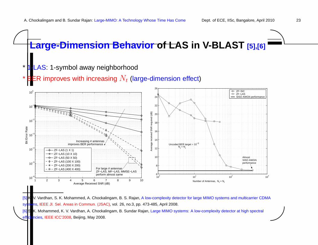
Large-Dimension Behavior of LAS in V-BLAST [5],[6]
* 1-LAS: 1-symbol away neighborhood
* BER improves with increasing Nt (large-dimension effect)
1 2 3 4 5 6 7 8 9 1010
−6
10−5
10−4
10−3
10−2
10−1
100
Average Received SNR (dB)
Bit
Err
or R
ate
ZF−LAS (1 X 1)ZF−LAS (10 X 10)ZF−LAS (50 X 50)ZF−LAS (100 X 100)ZF−LAS (200 X 200)ZF−LAS (400 X 400)
Increasing # antennasimproves BER performance
For large # antennasZF−LAS, MF−LAS, MMSE−LASperform almost same
100
101
102
103
6
8
10
12
14
16
18
20
22
24
26
= NNumber of Antennas, t N r
Ave
rage
rec
eive
d S
NR
req
uire
d (d
B)
ZF−SICZF−LASSISO AWGN performance
Uncoded BER target = 10−3
Nt = N
r
Almost SISO AWGN performance
——————[5] K. V. Vardhan, S. K. Mohammed, A. Chockalingam, B. S. Rajan, A low-complexity detector for large MIMO systems and multicarrier CDMA
systems, IEEE Jl. Sel. Areas in Commun. (JSAC), vol. 26, no.3, pp. 473-485, April 2008.
[6] S. K. Mohammed, K. V. Vardhan, A. Chockalingam, B. Sundar Rajan, Large MIMO systems: A low-complexity detector at high spectral
efficiencies, IEEE ICC’2008, Beijing, May 2008.
A. Chockalingam and B. Sundar Rajan: Large-MIMO: A Technology Whose Time Has Come Dept. of ECE, IISc, Bangalore, April 2010 24'
&
$
%
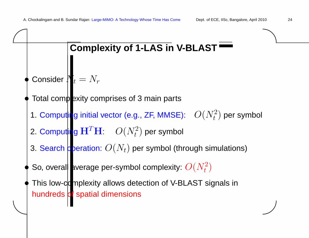
Complexity of 1-LAS in V-BLAST
• Consider Nt = Nr
• Total complexity comprises of 3 main parts
1. Computing initial vector (e.g., ZF, MMSE): O(N 2t ) per symbol
2. Computing HTH: O(N 2t ) per symbol
3. Search operation: O(Nt) per symbol (through simulations)
• So, overall average per-symbol complexity: O(N 2t )
• This low-complexity allows detection of V-BLAST signals inhundreds of spatial dimensions
A. Chockalingam and B. Sundar Rajan: Large-MIMO: A Technology Whose Time Has Come Dept. of ECE, IISc, Bangalore, April 2010 25'
&
$
%
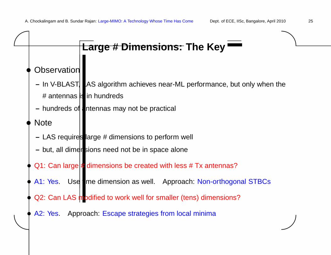
Large # Dimensions: The Key
• Observation
– In V-BLAST, LAS algorithm achieves near-ML performance, but only when the
# antennas is in hundreds
– hundreds of antennas may not be practical
• Note
– LAS requires large # dimensions to perform well
– but, all dimensions need not be in space alone
• Q1: Can large # dimensions be created with less # Tx antennas?
• A1: Yes. Use time dimension as well. Approach: Non-orthogonal STBCs
• Q2: Can LAS modified to work well for smaller (tens) dimensions?
• A2: Yes. Approach: Escape strategies from local minima
A. Chockalingam and B. Sundar Rajan: Large-MIMO: A Technology Whose Time Has Come Dept. of ECE, IISc, Bangalore, April 2010 26'
&
$
%
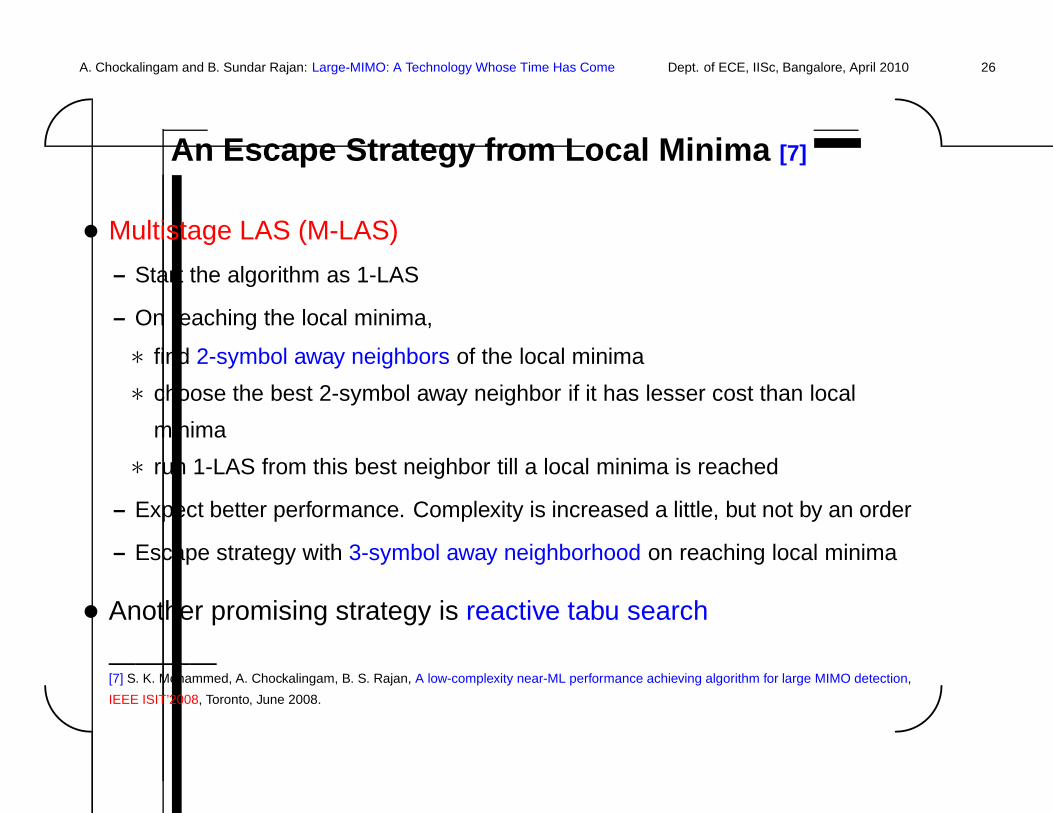
An Escape Strategy from Local Minima [7]
• Multistage LAS (M-LAS)
– Start the algorithm as 1-LAS
– On reaching the local minima,
∗ find 2-symbol away neighbors of the local minima
∗ choose the best 2-symbol away neighbor if it has lesser cost than local
minima
∗ run 1-LAS from this best neighbor till a local minima is reached
– Expect better performance. Complexity is increased a little, but not by an order
– Escape strategy with 3-symbol away neighborhood on reaching local minima
• Another promising strategy is reactive tabu search
————[7] S. K. Mohammed, A. Chockalingam, B. S. Rajan, A low-complexity near-ML performance achieving algorithm for large MIMO detection,
IEEE ISIT’2008, Toronto, June 2008.
A. Chockalingam and B. Sundar Rajan: Large-MIMO: A Technology Whose Time Has Come Dept. of ECE, IISc, Bangalore, April 2010 27'
&
$
%
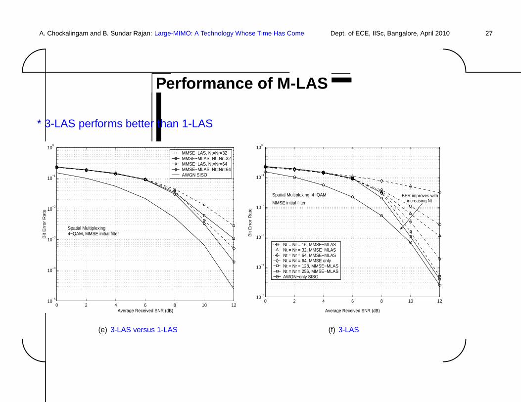
Performance of M-LAS
* 3-LAS performs better than 1-LAS
0 2 4 6 8 10 1210
−5
10−4
10−3
10−2
10−1
100
Average Received SNR (dB)
Bit
Err
or
Ra
te
MMSE−LAS, Nt=Nr=32MMSE−MLAS, Nt=Nr=32MMSE−LAS, Nt=Nr=64MMSE−MLAS, Nt=Nr=64AWGN SISO
Spatial Multiplexing4−QAM, MMSE initial filter
(e) 3-LAS versus 1-LAS
0 2 4 6 8 10 1210
−5
10−4
10−3
10−2
10−1
100
Average Received SNR (dB)
Bit
Err
or
Ra
te
Nt = Nr = 16, MMSE−MLASNt = Nr = 32, MMSE−MLASNt = Nr = 64, MMSE−MLASNt = Nr = 64, MMSE onlyNt = Nr = 128, MMSE−MLASNt = Nr = 256, MMSE−MLASAWGN−only SISO
Spatial Multiplexing, 4−QAM
MMSE initial filter
BER improves withincreasing Nt
(f) 3-LAS
A. Chockalingam and B. Sundar Rajan: Large-MIMO: A Technology Whose Time Has Come Dept. of ECE, IISc, Bangalore, April 2010 28'
&
$
%
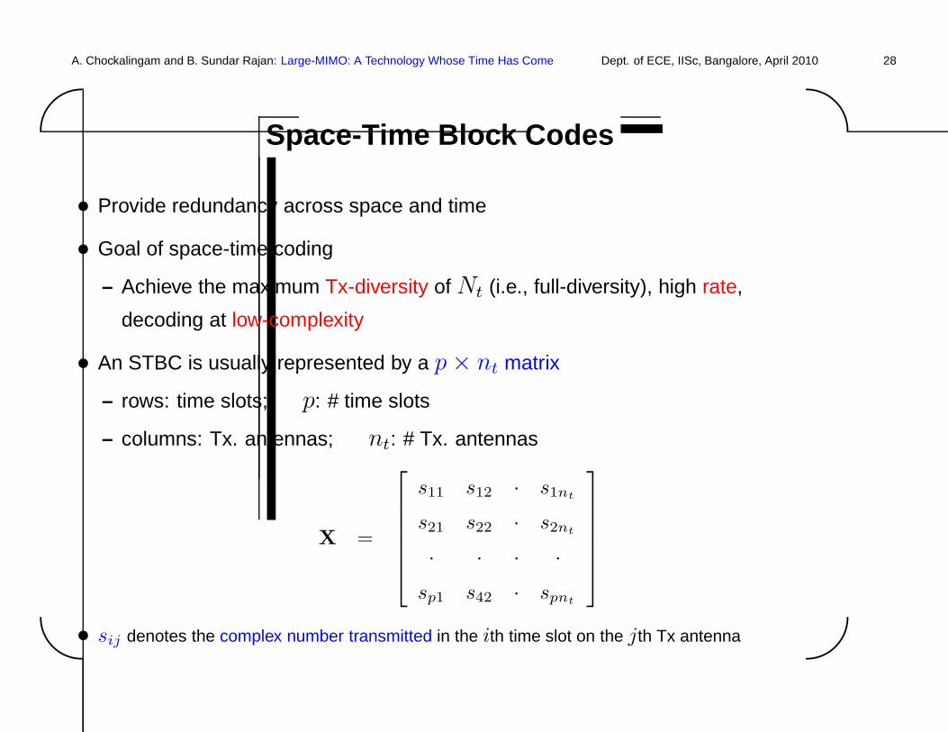
Space-Time Block Codes
• Provide redundancy across space and time
• Goal of space-time coding
– Achieve the maximum Tx-diversity of Nt (i.e., full-diversity), high rate,
decoding at low-complexity
• An STBC is usually represented by a p × nt matrix
– rows: time slots; p: # time slots
– columns: Tx. antennas; nt: # Tx. antennas
X =
s11 s12 · s1nt
s21 s22 · s2nt
· · · ·sp1 s42 · spnt
• sij denotes the complex number transmitted in the ith time slot on the jth Tx antenna
A. Chockalingam and B. Sundar Rajan: Large-MIMO: A Technology Whose Time Has Come Dept. of ECE, IISc, Bangalore, April 2010 29'
&
$
%
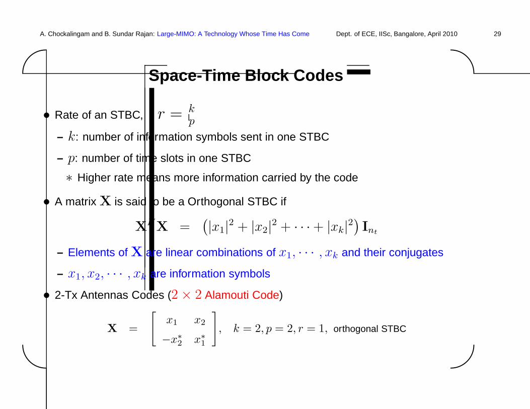
Space-Time Block Codes
• Rate of an STBC, r = kp
– k: number of information symbols sent in one STBC
– p: number of time slots in one STBC
∗ Higher rate means more information carried by the code
• A matrix X is said to be a Orthogonal STBC if
XHX =(|x1|2 + |x2|2 + · · · + |xk|2
)Int
– Elements of X are linear combinations of x1, · · · , xk and their conjugates
– x1, x2, · · · , xk are information symbols
• 2-Tx Antennas Codes (2 × 2 Alamouti Code)
X =
[x1 x2
−x∗2 x∗
1
], k = 2, p = 2, r = 1, orthogonal STBC

A. Chockalingam and B. Sundar Rajan: Large-MIMO: A Technology Whose Time Has Come Dept. of ECE, IISc, Bangalore, April 2010 30'
&
$
%
Linear-Complexity Decoding of OSTBCs
• Consider Alamouti code with nt = 2, nr = 1
• Received signal in ith slot, yi, i = 1, 2, is
y1 = h1x1 + h2x2 + n1
y2 = −h1x∗2 + h2x
∗1 + n2
• ML decoding amounts to
– computing
x1 = y1h∗1 + y∗
2h2
x2 = y1h∗2 − y∗
2h1
– decoding x1 by finding the symbol in the constellation that is closest to x1
– and decoding x2 by finding the symbol that is closest to x2
• This decoding feature is called Single-Symbol Decodability (SSD)
A. Chockalingam and B. Sundar Rajan: Large-MIMO: A Technology Whose Time Has Come Dept. of ECE, IISc, Bangalore, April 2010 31'
&
$
%
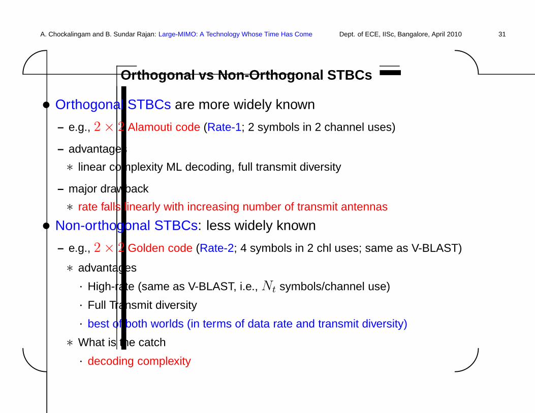
Orthogonal vs Non-Orthogonal STBCs
• Orthogonal STBCs are more widely known
– e.g., 2 × 2 Alamouti code (Rate-1; 2 symbols in 2 channel uses)
– advantages
∗ linear complexity ML decoding, full transmit diversity
– major drawback
∗ rate falls linearly with increasing number of transmit antennas
• Non-orthogonal STBCs: less widely known
– e.g., 2 × 2 Golden code (Rate-2; 4 symbols in 2 chl uses; same as V-BLAST)
∗ advantages
· High-rate (same as V-BLAST, i.e., Nt symbols/channel use)
· Full Transmit diversity
· best of both worlds (in terms of data rate and transmit diversity)
∗ What is the catch
· decoding complexity
A. Chockalingam and B. Sundar Rajan: Large-MIMO: A Technology Whose Time Has Come Dept. of ECE, IISc, Bangalore, April 2010 32'
&
$
%
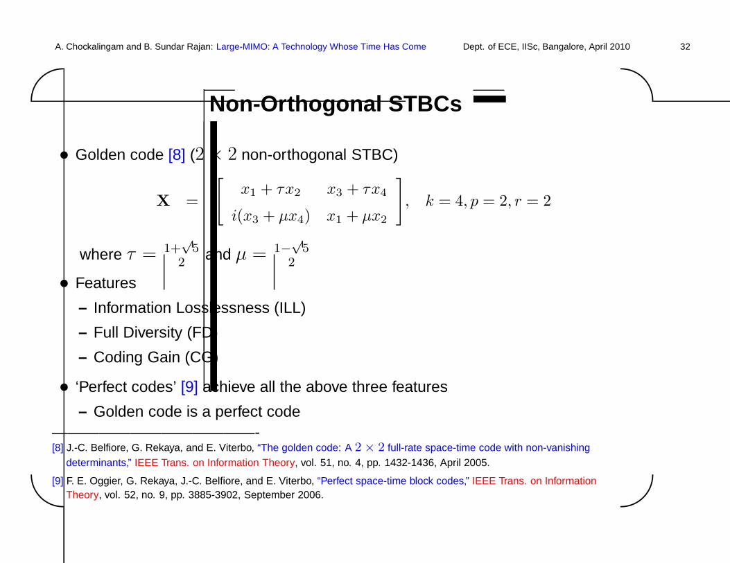
Non-Orthogonal STBCs
• Golden code [8] (2 × 2 non-orthogonal STBC)
X =
[x1 + τx2 x3 + τx4
i(x3 + µx4) x1 + µx2
], k = 4, p = 2, r = 2
where τ = 1+√
52
and µ = 1−√
52
• Features
– Information Losslessness (ILL)
– Full Diversity (FD)
– Coding Gain (CG)
• ‘Perfect codes’ [9] achieve all the above three features
– Golden code is a perfect code—————————————-[8] J.-C. Belfiore, G. Rekaya, and E. Viterbo, “The golden code: A 2 × 2 full-rate space-time code with non-vanishing
determinants,” IEEE Trans. on Information Theory, vol. 51, no. 4, pp. 1432-1436, April 2005.
[9] F. E. Oggier, G. Rekaya, J.-C. Belfiore, and E. Viterbo, “Perfect space-time block codes,” IEEE Trans. on InformationTheory, vol. 52, no. 9, pp. 3885-3902, September 2006.
A. Chockalingam and B. Sundar Rajan: Large-MIMO: A Technology Whose Time Has Come Dept. of ECE, IISc, Bangalore, April 2010 33'
&
$
%
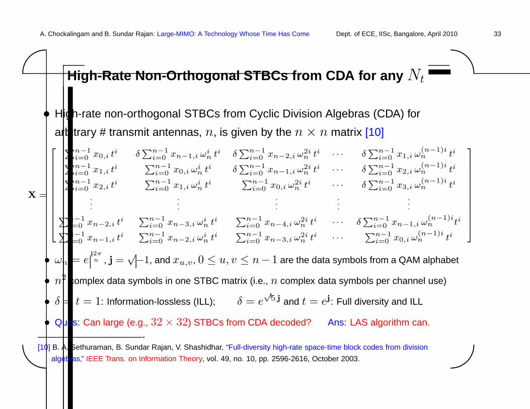
High-Rate Non-Orthogonal STBCs from CDA for any Nt
• High-rate non-orthogonal STBCs from Cyclic Division Algebras (CDA) for
arbitrary # transmit antennas, n, is given by the n × n matrix [10]
X =
2
6
6
6
6
6
6
6
6
6
6
6
4
Pn−1i=0 x0,i ti δ
Pn−1i=0 xn−1,i ωi
n ti δPn−1
i=0 xn−2,i ω2in ti · · · δ
Pn−1i=0 x1,i ω
(n−1)in ti
Pn−1i=0 x1,i ti
Pn−1i=0 x0,i ωi
n ti δPn−1
i=0 xn−1,i ω2in ti · · · δ
Pn−1i=0 x2,i ω
(n−1)in ti
Pn−1i=0 x2,i ti
Pn−1i=0 x1,i ωi
n tiPn−1
i=0 x0,i ω2in ti · · · δ
Pn−1i=0 x3,i ω
(n−1)in ti
.
.
....
.
.
....
.
.
.Pn−1
i=0 xn−2,i tiPn−1
i=0 xn−3,i ωin ti
Pn−1i=0 xn−4,i ω2i
n ti · · · δPn−1
i=0 xn−1,i ω(n−1)in ti
Pn−1i=0 xn−1,i ti
Pn−1i=0 xn−2,i ωi
n tiPn−1
i=0 xn−3,i ω2in ti · · ·
Pn−1i=0 x0,i ω
(n−1)in ti
3
7
7
7
7
7
7
7
7
7
7
7
5
• ωn = ej2π
n , j =√−1, and xu,v , 0 ≤ u, v ≤ n− 1 are the data symbols from a QAM alphabet
• n2 complex data symbols in one STBC matrix (i.e., n complex data symbols per channel use)
• δ = t = 1: Information-lossless (ILL); δ = e√
5 j and t = ej: Full diversity and ILL
• Ques: Can large (e.g., 32 × 32) STBCs from CDA decoded? Ans: LAS algorithm can.
———————————-[10] B. A. Sethuraman, B. Sundar Rajan, V. Shashidhar, “Full-diversity high-rate space-time block codes from division
algebras,” IEEE Trans. on Information Theory, vol. 49, no. 10, pp. 2596-2616, October 2003.
A. Chockalingam and B. Sundar Rajan: Large-MIMO: A Technology Whose Time Has Come Dept. of ECE, IISc, Bangalore, April 2010 34'
&
$
%
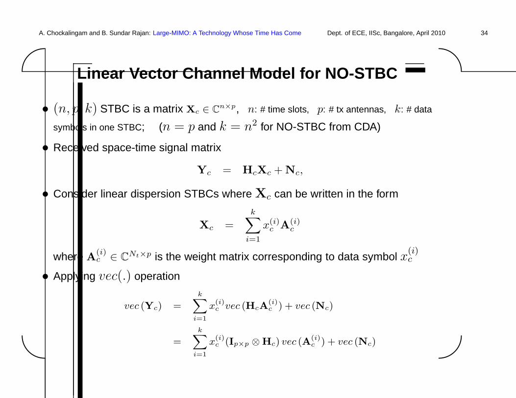
Linear Vector Channel Model for NO-STBC
• (n, p, k) STBC is a matrix Xc ∈ Cn×p, n: # time slots, p: # tx antennas, k: # data
symbols in one STBC; (n = p and k = n2 for NO-STBC from CDA)
• Received space-time signal matrix
Yc = HcXc + Nc,
• Consider linear dispersion STBCs where Xc can be written in the form
Xc =k∑
i=1
x(i)c A(i)
c
where A(i)c ∈ C
Nt×p is the weight matrix corresponding to data symbol x(i)c
• Applying vec(.) operation
vec (Yc) =
kX
i=1
x(i)c vec (HcA
(i)c ) + vec (Nc)
=k
X
i=1
x(i)c (Ip×p ⊗ Hc) vec (A(i)
c ) + vec (Nc)
A. Chockalingam and B. Sundar Rajan: Large-MIMO: A Technology Whose Time Has Come Dept. of ECE, IISc, Bangalore, April 2010 35'
&
$
%
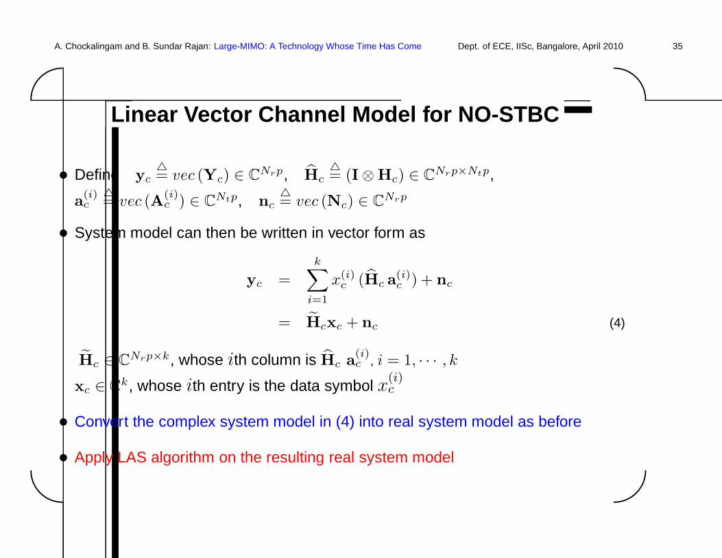
Linear Vector Channel Model for NO-STBC
• Define yc△= vec (Yc) ∈ C
Nrp, Hc△= (I⊗Hc) ∈ C
Nrp×Ntp,
a(i)c
△= vec (A
(i)c ) ∈ C
Ntp, nc△= vec (Nc) ∈ C
Nrp
• System model can then be written in vector form as
yc =k∑
i=1
x(i)c (Hc a(i)
c ) + nc
= Hcxc + nc (4)
Hc ∈ CNrp×k, whose ith column is Hc a
(i)c , i = 1, · · · , k
xc ∈ Ck, whose ith entry is the data symbol x
(i)c
• Convert the complex system model in (4) into real system model as before
• Apply LAS algorithm on the resulting real system model
A. Chockalingam and B. Sundar Rajan: Large-MIMO: A Technology Whose Time Has Come Dept. of ECE, IISc, Bangalore, April 2010 36'
&
$
%
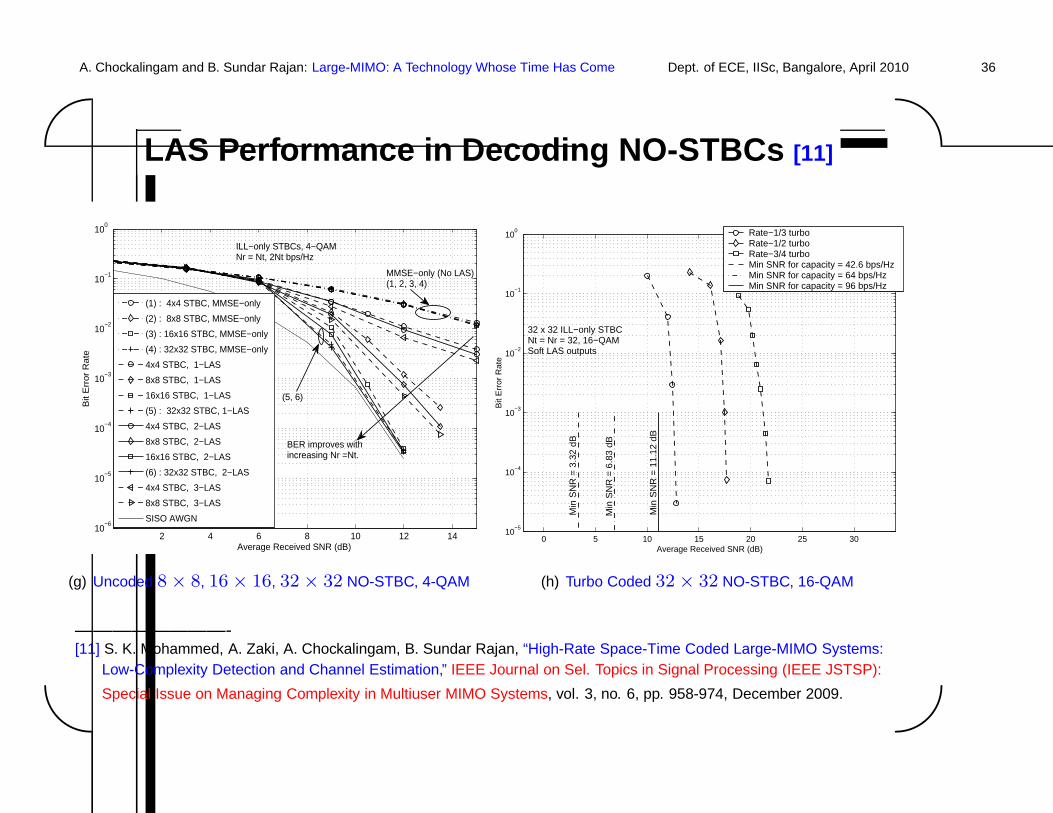
LAS Performance in Decoding NO-STBCs [11]
2 4 6 8 10 12 1410
−6
10−5
10−4
10−3
10−2
10−1
100
Average Received SNR (dB)
Bit
Err
or
Ra
te
ILL−only STBCs, 4−QAM Nr = Nt, 2Nt bps/Hz
(1) : 4x4 STBC, MMSE−only
(2) : 8x8 STBC, MMSE−only
(3) : 16x16 STBC, MMSE−only
(4) : 32x32 STBC, MMSE−only
4x4 STBC, 1−LAS
8x8 STBC, 1−LAS
16x16 STBC, 1−LAS
(5) : 32x32 STBC, 1−LAS
4x4 STBC, 2−LAS
8x8 STBC, 2−LAS
16x16 STBC, 2−LAS
(6) : 32x32 STBC, 2−LAS
4x4 STBC, 3−LAS
8x8 STBC, 3−LAS
SISO AWGN
(5, 6)
BER improves withincreasing Nr =Nt.
MMSE−only (No LAS)(1, 2, 3, 4)
(g) Uncoded 8 × 8, 16 × 16, 32 × 32 NO-STBC, 4-QAM
0 5 10 15 20 25 3010
−5
10−4
10−3
10−2
10−1
100
Average Received SNR (dB)
Bit
Err
or R
ate
Rate−1/3 turboRate−1/2 turbo Rate−3/4 turboMin SNR for capacity = 42.6 bps/HzMin SNR for capacity = 64 bps/HzMin SNR for capacity = 96 bps/Hz
Min
SN
R =
6.8
3 dB
Min
SN
R =
11.
12 d
B
32 x 32 ILL−only STBCNt = Nr = 32, 16−QAMSoft LAS outputs
Min
SN
R =
3.3
2 dB
(h) Turbo Coded 32 × 32 NO-STBC, 16-QAM
————————-[11] S. K. Mohammed, A. Zaki, A. Chockalingam, B. Sundar Rajan, “High-Rate Space-Time Coded Large-MIMO Systems:
Low-Complexity Detection and Channel Estimation,” IEEE Journal on Sel. Topics in Signal Processing (IEEE JSTSP):
Special Issue on Managing Complexity in Multiuser MIMO Systems, vol. 3, no. 6, pp. 958-974, December 2009.
A. Chockalingam and B. Sundar Rajan: Large-MIMO: A Technology Whose Time Has Come Dept. of ECE, IISc, Bangalore, April 2010 37'
&
$
%
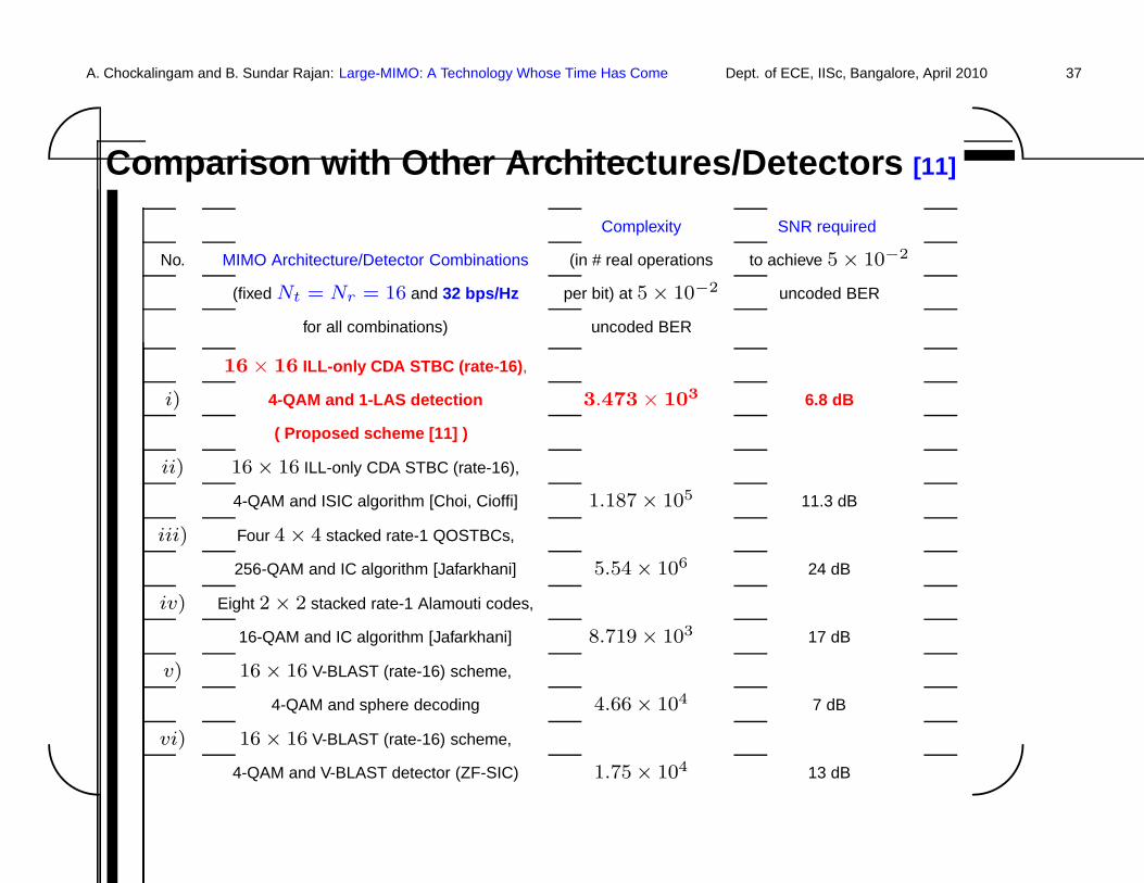
Comparison with Other Architectures/Detectors [11]
Complexity SNR required
No. MIMO Architecture/Detector Combinations (in # real operations to achieve 5 × 10⁻²
(fixed Nt = Nr = 16 and 32 bps/Hz per bit) at 5 × 10⁻² uncoded BER
for all combinations) uncoded BER
16 × 16 ILL-only CDA STBC (rate-16) ,
i) 4-QAM and 1-LAS detection 3.473 × 10³ 6.8 dB
( Proposed scheme [11] )
ii) 16 × 16 ILL-only CDA STBC (rate-16),
4-QAM and ISIC algorithm [Choi, Cioffi] 1.187 × 10⁵ 11.3 dB
iii) Four 4 × 4 stacked rate-1 QOSTBCs,
256-QAM and IC algorithm [Jafarkhani] 5.54 × 10⁶ 24 dB
iv) Eight 2 × 2 stacked rate-1 Alamouti codes,
16-QAM and IC algorithm [Jafarkhani] 8.719 × 10³ 17 dB
v) 16 × 16 V-BLAST (rate-16) scheme,
4-QAM and sphere decoding 4.66 × 10⁴ 7 dB
vi) 16 × 16 V-BLAST (rate-16) scheme,
4-QAM and V-BLAST detector (ZF-SIC) 1.75 × 10⁴ 13 dB
A. Chockalingam and B. Sundar Rajan: Large-MIMO: A Technology Whose Time Has Come Dept. of ECE, IISc, Bangalore, April 2010 38'
&
$
%
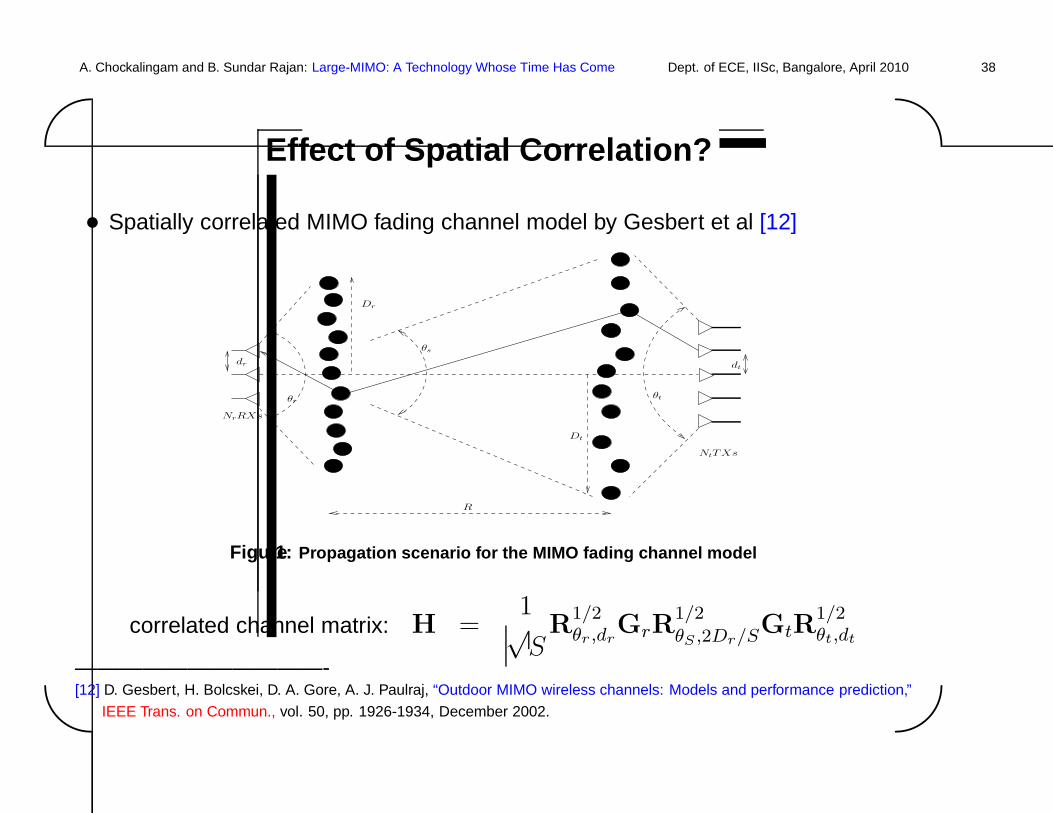
Effect of Spatial Correlation?
• Spatially correlated MIMO fading channel model by Gesbert et al [12]
NtTXs
dt
θt
Dt
R
θs
Dr
θr
NrRXs
dr
Figure1: Propagation scenario for the MIMO fading channel model
correlated channel matrix: H =1√S
R1/2θr ,dr
GrR1/2θS ,2Dr/SGtR
1/2θt,dt
———————————-[12] D. Gesbert, H. Bolcskei, D. A. Gore, A. J. Paulraj, “Outdoor MIMO wireless channels: Models and performance prediction,”
IEEE Trans. on Commun., vol. 50, pp. 1926-1934, December 2002.
A. Chockalingam and B. Sundar Rajan: Large-MIMO: A Technology Whose Time Has Come Dept. of ECE, IISc, Bangalore, April 2010 39'
&
$
%
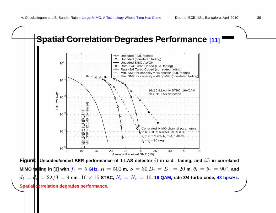
Spatial Correlation Degrades Performance [11]
5 10 15 20 25 30 35 40 45 5010
−5
10−4
10−3
10−2
10−1
100
Average Received SNR (dB)
Bit
Err
or R
ate Uncoded (i.i.d. fading)Uncoded (correlated fading)Uncoded SISO AWGNRate−3/4 Turbo Coded (i.i.d. fading)Rate−3/4 Turbo Coded (correlated fading)Min. SNR for capacity = 48 bps/Hz (i.i.d. fading)Min. SNR for capacity = 48 bps/Hz (correlated fading)
16x16 ILL−only STBC, 16−QAMNt = Nr, LAS detection
Correlated MIMO channel parameters:
dt = d
r = 4 cm. D
r = D
t = 20 m.
fc = 5 GHz, R = 500 m, S = 30
θt = θ
r = 90 deg.
Min
. SN
R =
11.
1 dB
(i.i.
d.)
Min
. SN
R =
12.
6 dB
(cor
rela
ted)
Figure2: Uncoded/coded BER performance of 1-LAS detector i) in i.i.d. fading, and ii) in correlated
MIMO fading in [3] with fc = 5 GHz, R = 500 m, S = 30,Dt = Dr = 20 m, θt = θr = 90◦, and
dt = dr = 2λ/3 = 4 cm. 16 × 16 STBC, Nt = Nr = 16, 16-QAM, rate-3/4 turbo code, 48 bps/Hz .
Spatial correlation degrades performance .
A. Chockalingam and B. Sundar Rajan: Large-MIMO: A Technology Whose Time Has Come Dept. of ECE, IISc, Bangalore, April 2010 40'
&
$
%
Increasing # Receive Dimensions Helps! [11]
5 10 15 20 25 30 35 40 45 5010
−5
10−4
10−3
10−2
10−1
100
Average Received SNR (dB)
Bit
Err
or R
ate
Nt = Nr = 12, uncodedNt = 12, Nr = 18, uncodedUncoded SISO AWGNNt = Nr = 12, rate−3/4 turbo codedNt = 12, Nr = 18, rate−3/4 turbo codedMin. SNR for Capacity = 36 bps/Hz (Nt = Nr = 12)Min. SNR for capacity = 36 bps/Hz (Nt = 12, Nr = 18)
12x12 ILL−only STBC, 16−QAMNt = 12, Nr = 12,18, 1−LAS detection
Correlated MIMO chl parameters:
Nrd
r = 72 cm, d
t = d
r
Dr = D
t = 20 m
fc = 5 GHz, R = 500 m, S = 30
θt = θ
r = 90 deg.
Min
. SN
R =
12.
6 dB
(Nr =
12)
Min
. SN
R =
9.4
dB
(Nr =
18)
Figure3: Effect of Nr > Nt in correlated MIMO fading in [3] keeping Nrdr constant and dt = dr .
Nrdr = 72 cm, fc = 5 GHz, R = 500 m, S = 30, Dt = Dr = 20 m, θt = θr = 90◦, 12 × 12
ILL-only STBC, Nt = 12, Nr = 12, 18, 16-QAM, rate-3/4 turbo code, 36 bps/Hz . Increasing # receive
dimensions alleviates the loss due to spatial correlation .
A. Chockalingam and B. Sundar Rajan: Large-MIMO: A Technology Whose Time Has Come Dept. of ECE, IISc, Bangalore, April 2010 41'
&
$
%
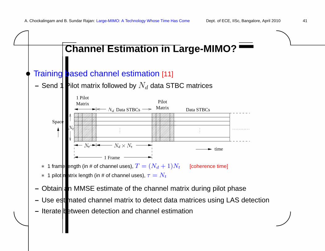
Channel Estimation in Large-MIMO?
• Training based channel estimation [11]
– Send 1 Pilot matrix followed by Nd data STBC matrices
��������
��������������������
������������������������������
����������������������������������������
����������
������������������������������
������������������������������������������������������������
����������
���
���
���
���
�������
���
����
��������������
����������
time
Data STBCs
Space
MatrixMatrixPilot
1 Pilot
Data STBCs
1 Frame
Nt Nt Nd �NtNd
∗ 1 frame length (in # of channel uses), T = (Nd + 1)Nt [coherence time]
∗ 1 pilot matrix length (in # of channel uses), τ = Nt
– Obtain an MMSE estimate of the channel matrix during pilot phase
– Use estimated channel matrix to detect data matrices using LAS detection
– Iterate between detection and channel estimation
A. Chockalingam and B. Sundar Rajan: Large-MIMO: A Technology Whose Time Has Come Dept. of ECE, IISc, Bangalore, April 2010 42'
&
$
%
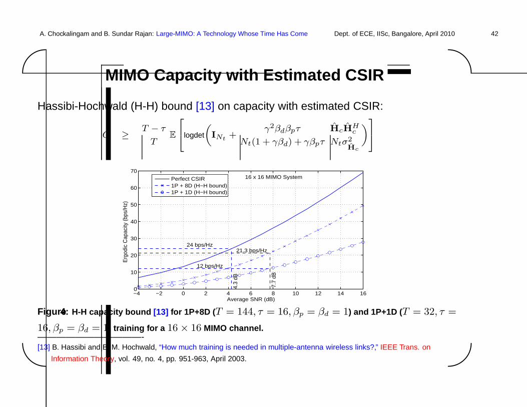
MIMO Capacity with Estimated CSIR
Hassibi-Hochwald (H-H) bound [13] on capacity with estimated CSIR:
C ≥ T − τ
TE
2
4logdet
„
INt+
γ2βdβpτ
Nt(1 + γβd) + γβpτ
HcHHc
Ntσ2Hc
«
3
5
−4 −2 0 2 4 6 8 10 12 14 160
10
20
30
40
50
60
70
Average SNR (dB)
Erg
odic
Cap
acity
(bps
/Hz)
Perfect CSIR1P + 8D (H−H bound)1P + 1D (H−H bound)
16 x 16 MIMO System
24 bps/Hz21.3 bps/Hz
12 bps/Hz7.
7 dB
4.3
dB
Figure4: H-H capacity bound [13] for 1P+8D (T = 144, τ = 16, βp = βd = 1) and 1P+1D (T = 32, τ =
16, βp = βd = 1) training for a 16 × 16 MIMO channel.———————————-[13] B. Hassibi and B. M. Hochwald, “How much training is needed in multiple-antenna wireless links?,” IEEE Trans. on
Information Theory, vol. 49, no. 4, pp. 951-963, April 2003.
A. Chockalingam and B. Sundar Rajan: Large-MIMO: A Technology Whose Time Has Come Dept. of ECE, IISc, Bangalore, April 2010 43'
&
$
%
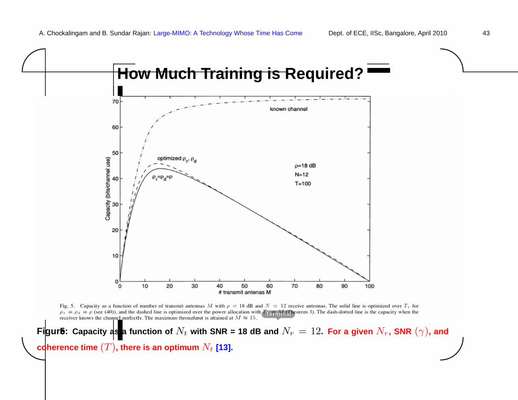
How Much Training is Required?
Figure5: Capacity as a function of Nt with SNR = 18 dB and Nr = 12. For a given Nr , SNR (γ), and
coherence time (T ), there is an optimum Nt [13] .
A. Chockalingam and B. Sundar Rajan: Large-MIMO: A Technology Whose Time Has Come Dept. of ECE, IISc, Bangalore, April 2010 44'
&
$
%
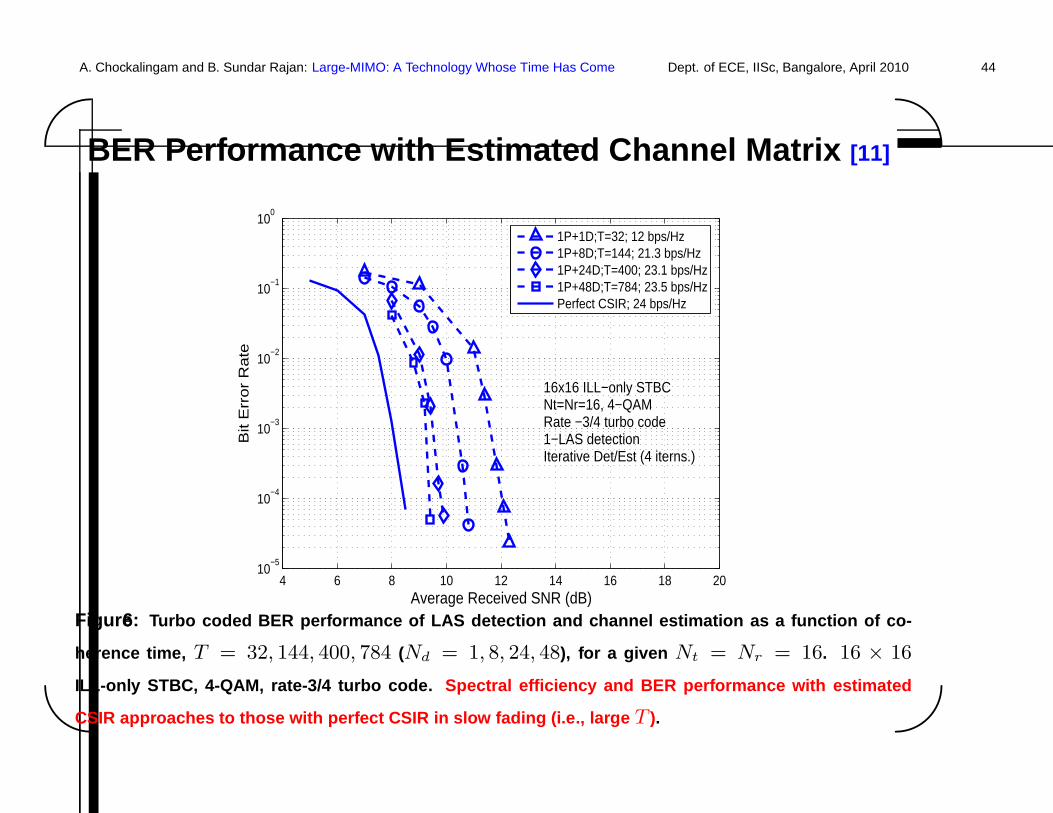
BER Performance with Estimated Channel Matrix [11]
4 6 8 10 12 14 16 18 2010
−5
10−4
10−3
10−2
10−1
100
Average Received SNR (dB)
Bit
Err
or
Ra
te
1P+1D;T=32; 12 bps/Hz1P+8D;T=144; 21.3 bps/Hz1P+24D;T=400; 23.1 bps/Hz1P+48D;T=784; 23.5 bps/HzPerfect CSIR; 24 bps/Hz
16x16 ILL−only STBCNt=Nr=16, 4−QAMRate −3/4 turbo code1−LAS detectionIterative Det/Est (4 iterns.)
Figure6: Turbo coded BER performance of LAS detection and channel est imation as a function of co-
herence time, T = 32, 144, 400, 784 (Nd = 1, 8, 24, 48), for a given Nt = Nr = 16. 16 × 16
ILL-only STBC, 4-QAM, rate-3/4 turbo code. Spectral efficiency and BER performance with estimated
CSIR approaches to those with perfect CSIR in slow fading (i. e., large T ).
A. Chockalingam and B. Sundar Rajan: Large-MIMO: A Technology Whose Time Has Come Dept. of ECE, IISc, Bangalore, April 2010 45'
&
$
%
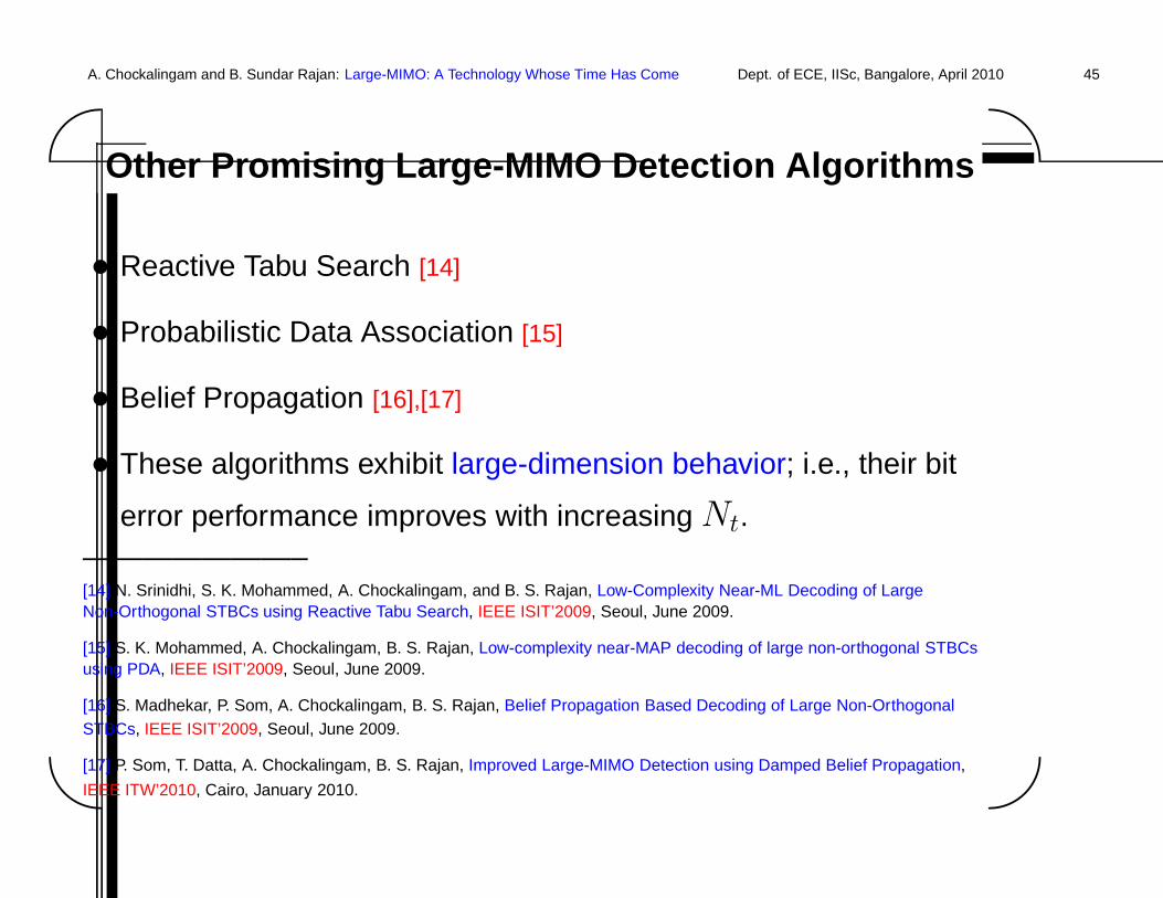
Other Promising Large-MIMO Detection Algorithms
• Reactive Tabu Search [14]
• Probabilistic Data Association [15]
• Belief Propagation [16],[17]
• These algorithms exhibit large-dimension behavior; i.e., their bit
error performance improves with increasing Nt.———————–[14] N. Srinidhi, S. K. Mohammed, A. Chockalingam, and B. S. Rajan, Low-Complexity Near-ML Decoding of LargeNon-Orthogonal STBCs using Reactive Tabu Search, IEEE ISIT’2009, Seoul, June 2009.
[15] S. K. Mohammed, A. Chockalingam, B. S. Rajan, Low-complexity near-MAP decoding of large non-orthogonal STBCsusing PDA, IEEE ISIT’2009, Seoul, June 2009.
[16] S. Madhekar, P. Som, A. Chockalingam, B. S. Rajan, Belief Propagation Based Decoding of Large Non-OrthogonalSTBCs, IEEE ISIT’2009, Seoul, June 2009.
[17] P. Som, T. Datta, A. Chockalingam, B. S. Rajan, Improved Large-MIMO Detection using Damped Belief Propagation,
IEEE ITW’2010, Cairo, January 2010.
A. Chockalingam and B. Sundar Rajan: Large-MIMO: A Technology Whose Time Has Come Dept. of ECE, IISc, Bangalore, April 2010 46'
&
$
%
Reactive Tabu Search
• Another iterative local search algorithm
– A metaheuristics algorithm
– cannot guarantee optimal solution, but generally gives near optimal solution
• Uses ‘tabu’ mechanism to escape from local minima or cycles
– Certain vectors are prohibited (made tabu) from becoming solution vectors for
certain number of iterations (called tabu period) depending on the search path
– This is meant to ensure efficient exploration of the search space
• The reactive part adapts the tabu period
A. Chockalingam and B. Sundar Rajan: Large-MIMO: A Technology Whose Time Has Come Dept. of ECE, IISc, Bangalore, April 2010 47'
&
$
%
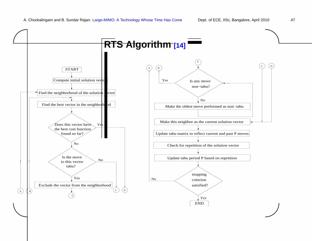
RTS Algorithm [14]
A B
C DA B
DC
Yes
START
Is the move to this vector
tabu?
found so far?the best cost function Does this vector have Yes
No
Yes
No
Is any move
non−tabu?
Make this neighbor as the current solution vector
Update tabu period P based on repetition
satisfied?
criterion
stopping
Yes
END
No
Make the oldest move performed as non−tabu
Find the neighborhood of the solution vector
NoFind the best vector in the neighborhood
Update tabu matrix to reflect current and past P moves
Check for repetition of the solution vector
Exclude the vector from the neighborhood
Compute initial solution vector
E
E
A. Chockalingam and B. Sundar Rajan: Large-MIMO: A Technology Whose Time Has Come Dept. of ECE, IISc, Bangalore, April 2010 48'
&
$
%
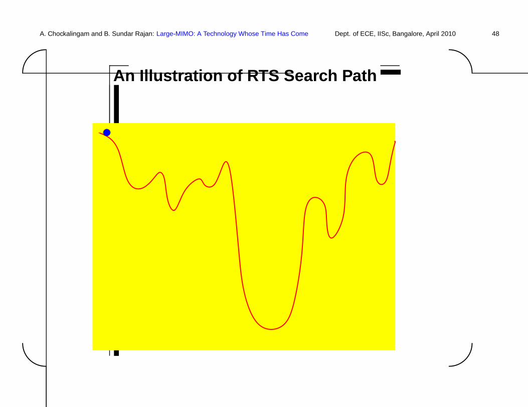
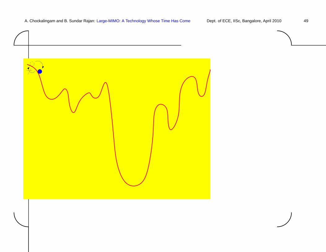
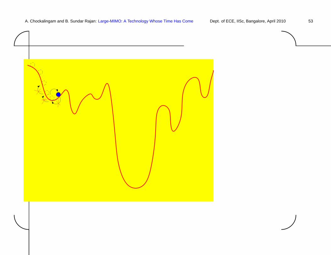
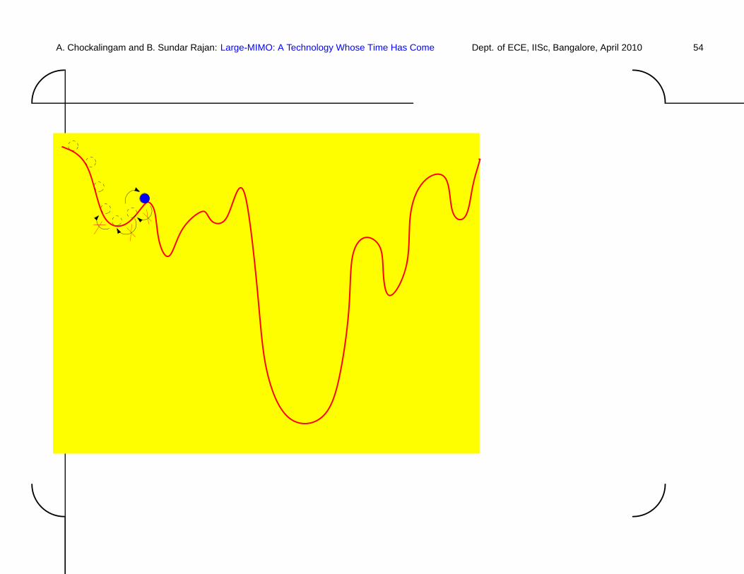
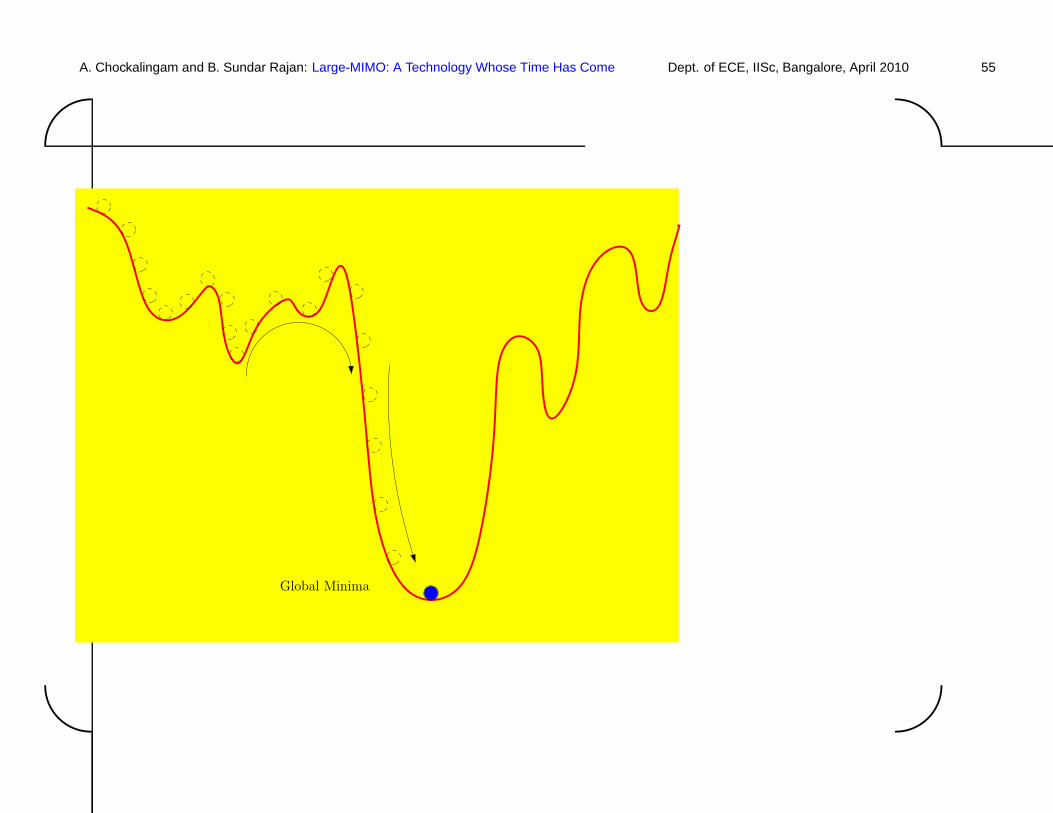
An Illustration of RTS Search Path
A. Chockalingam and B. Sundar Rajan: Large-MIMO: A Technology Whose Time Has Come Dept. of ECE, IISc, Bangalore, April 2010 49'
&
$
%

A. Chockalingam and B. Sundar Rajan: Large-MIMO: A Technology Whose Time Has Come Dept. of ECE, IISc, Bangalore, April 2010 50'
&
$
%

A. Chockalingam and B. Sundar Rajan: Large-MIMO: A Technology Whose Time Has Come Dept. of ECE, IISc, Bangalore, April 2010 51'
&
$
%

A. Chockalingam and B. Sundar Rajan: Large-MIMO: A Technology Whose Time Has Come Dept. of ECE, IISc, Bangalore, April 2010 52'
&
$
%
A. Chockalingam and B. Sundar Rajan: Large-MIMO: A Technology Whose Time Has Come Dept. of ECE, IISc, Bangalore, April 2010 53'
&
$
%
A. Chockalingam and B. Sundar Rajan: Large-MIMO: A Technology Whose Time Has Come Dept. of ECE, IISc, Bangalore, April 2010 54'
&
$
%
A. Chockalingam and B. Sundar Rajan: Large-MIMO: A Technology Whose Time Has Come Dept. of ECE, IISc, Bangalore, April 2010 55'
&
$
%
Global Minima
A. Chockalingam and B. Sundar Rajan: Large-MIMO: A Technology Whose Time Has Come Dept. of ECE, IISc, Bangalore, April 2010 56'
&
$
%
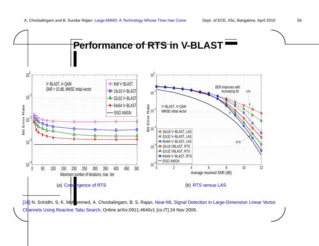
Performance of RTS in V-BLAST
0 50 100 150 200 250 300 350 400 450 50010
−4
10−3
10−2
10−1
100
Maximum number of iterations, max_iter
Bit E
rro
r R
ate
V−BLAST, 4−QAM SNR = 10 dB, MMSE initial vector
8x8 V−BLAST16x16 V−BLAST32x32 V−BLAST64x64 V−BLASTSISO AWGN
(a) Convergence of RTS
0 2 4 6 8 10 1210
−5
10−4
10−3
10−2
10−1
100
Average received SNR (dB)
Bit E
rro
r R
ate
16x16 V−BLAST, LAS32x32 V−BLAST, LAS64x64 V−BLAST, LAS16x16 VBLAST, RTS32x32 VBLAST, RTS64x64 V−BLAST, RTSSISO AWGN
V−BLAST, 4−QAMMMSE initial vector
BER improves withincreasing Nt LAS
RTS
(b) RTS versus LAS
——————–[18] N. Srinidhi, S. K. Mohammed, A. Chockalingam, B. S. Rajan, Near-ML Signal Detection in Large-Dimension Linear Vector
Channels Using Reactive Tabu Search, Online arXiv:0911.4640v1 [cs.IT] 24 Nov 2009.
A. Chockalingam and B. Sundar Rajan: Large-MIMO: A Technology Whose Time Has Come Dept. of ECE, IISc, Bangalore, April 2010 57'
&
$
%
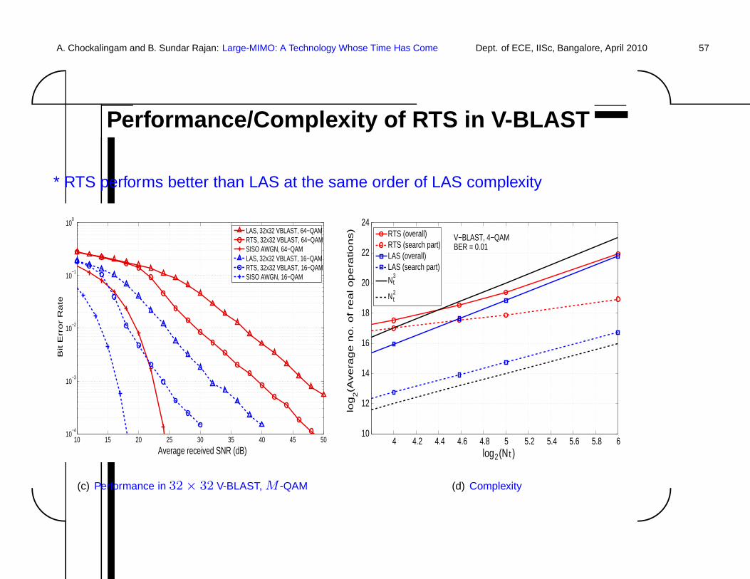
Performance/Complexity of RTS in V-BLAST
* RTS performs better than LAS at the same order of LAS complexity
10 15 20 25 30 35 40 45 5010
−4
10−3
10−2
10−1
100
Average received SNR (dB)
Bit E
rro
r R
ate
LAS, 32x32 VBLAST, 64−QAMRTS, 32x32 VBLAST, 64−QAMSISO AWGN, 64−QAMLAS, 32x32 VBLAST, 16−QAMRTS, 32x32 VBLAST, 16−QAMSISO AWGN, 16−QAM
(c) Performance in 32 × 32 V-BLAST, M -QAM
4 4.2 4.4 4.6 4.8 5 5.2 5.4 5.6 5.8 610
12
14
16
18
20
22
24
log2(N t )
log
2(A
ve
rag
e n
o.
of
rea
l o
pe
ratio
ns)
V−BLAST, 4−QAMBER = 0.01
RTS (overall)RTS (search part)LAS (overall)LAS (search part)
Nt3
N t2
(d) Complexity
A. Chockalingam and B. Sundar Rajan: Large-MIMO: A Technology Whose Time Has Come Dept. of ECE, IISc, Bangalore, April 2010 58'
&
$
%
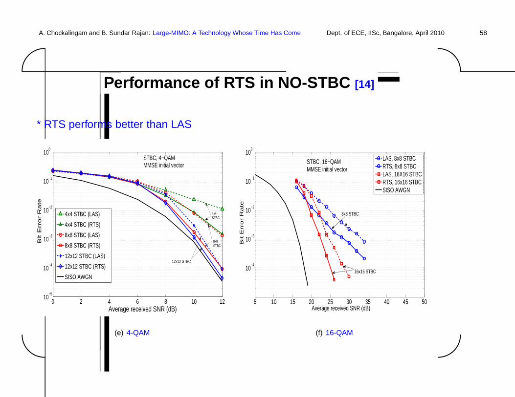
Performance of RTS in NO-STBC [14]
* RTS performs better than LAS
0 2 4 6 8 10 1210
−5
10−4
10−3
10−2
10−1
100
Average received SNR (dB)
Bit E
rro
r R
ate
4x4 STBC (LAS)
4x4 STBC (RTS)
8x8 STBC (LAS)
8x8 STBC (RTS)
12x12 STBC (LAS)
12x12 STBC (RTS)
SISO AWGN
8x8 STBC
STBC, 4−QAMMMSE initial vector
12x12 STBC
4x4 STBC
(e) 4-QAM
5 10 15 20 25 30 35 40 45 50
10−4
10−3
10−2
10−1
100
Average received SNR (dB)
Bit E
rro
r R
ate
LAS, 8x8 STBCRTS, 8x8 STBCLAS, 16X16 STBCRTS, 16x16 STBCSISO AWGN
16x16 STBC
8x8 STBC
STBC, 16−QAMMMSE initial vector
(f) 16-QAM
A. Chockalingam and B. Sundar Rajan: Large-MIMO: A Technology Whose Time Has Come Dept. of ECE, IISc, Bangalore, April 2010 59'
&
$
%
Probabilistic Data Association
• Originally developed for target tracking
• Used in digital communications recently
• PDA
– A reduced complexity alternative to a posteriori probability (APP)
detector/decoder/equalizer.
– Has been applied in
∗ Multiuser detection in CDMA (Luo et al 2001, Huang and
Zhang 2004, Tan and Rasmussen 2006)
∗ Turbo equalization (Yin et al 2004)
A. Chockalingam and B. Sundar Rajan: Large-MIMO: A Technology Whose Time Has Come Dept. of ECE, IISc, Bangalore, April 2010 60'
&
$
%
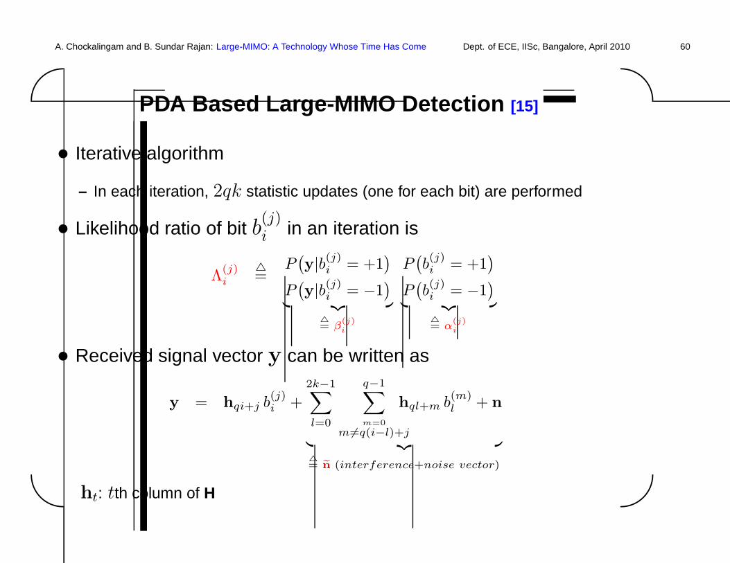
PDA Based Large-MIMO Detection [15]
• Iterative algorithm
– In each iteration, 2qk statistic updates (one for each bit) are performed
• Likelihood ratio of bit b(j)i in an iteration is
Λ(j)i
△=
P(y|b(j)
i = +1)
P(y|b(j)
i = −1)
︸ ︷︷ ︸△= β
(j)i
P(b(j)i = +1
)
P(b(j)i = −1
)︸ ︷︷ ︸
△= α
(j)i
• Received signal vector y can be written as
y = hqi+j b(j)i +
2k−1∑
l=0
q−1∑
m=0
m 6=q(i−l)+j
hql+m b(m)l + n
︸ ︷︷ ︸△= en (interference+noise vector)
ht: tth column of H
A. Chockalingam and B. Sundar Rajan: Large-MIMO: A Technology Whose Time Has Come Dept. of ECE, IISc, Bangalore, April 2010 61'
&
$
%
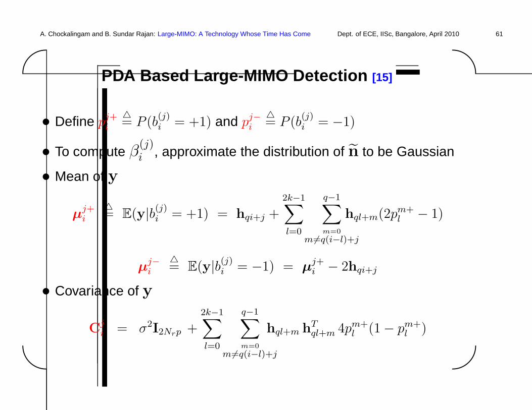
PDA Based Large-MIMO Detection [15]
• Define pj+i
△= P (b
(j)i = +1) and p
j−i
△= P (b
(j)i = −1)
• To compute β(j)i , approximate the distribution of n to be Gaussian
• Mean of y
µj+i
△= E(y|b(j)
i = +1) = hqi+j +2k−1∑
l=0
q−1∑
m=0
m 6=q(i−l)+j
hql+m(2pm+l − 1)
µj−i
△= E(y|b(j)
i = −1) = µj+i − 2hqi+j
• Covariance of y
Cji = σ2I2Nrp +
2k−1∑
l=0
q−1∑
m=0
m 6=q(i−l)+j
hql+m hTql+m 4pm+
l (1 − pm+l )
A. Chockalingam and B. Sundar Rajan: Large-MIMO: A Technology Whose Time Has Come Dept. of ECE, IISc, Bangalore, April 2010 62'
&
$
%
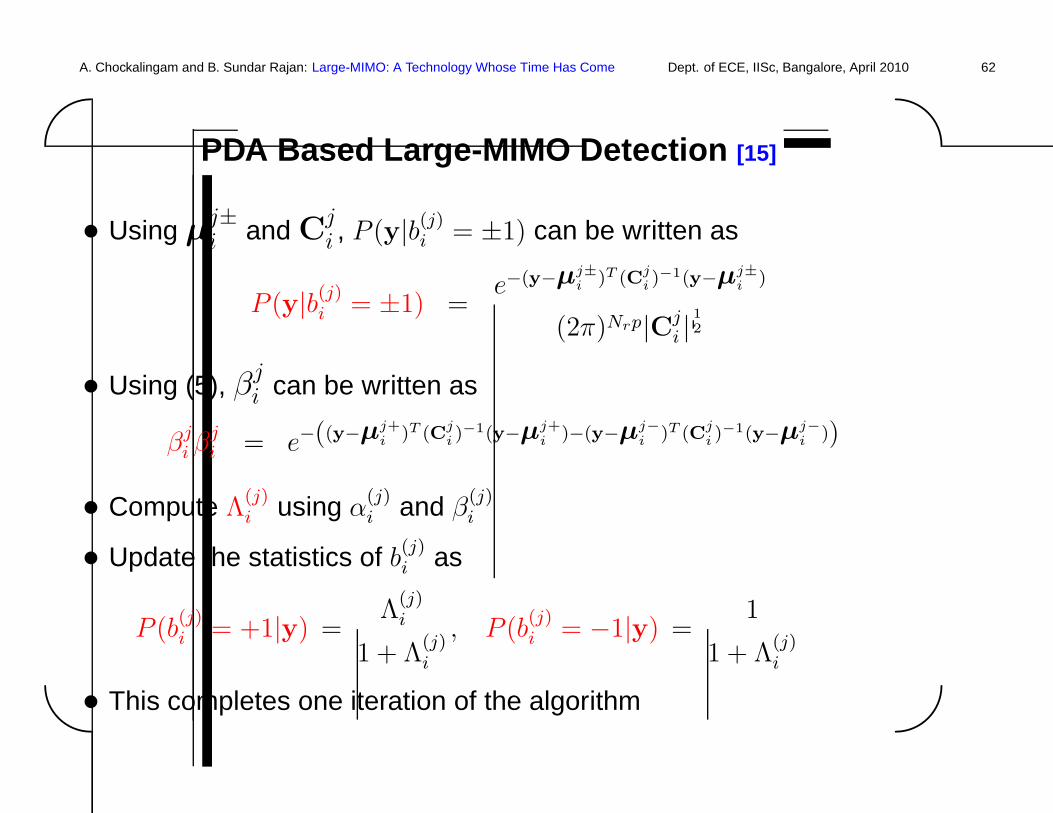
PDA Based Large-MIMO Detection [15]
• Using µj±i and C
ji , P (y|b(j)
i = ±1) can be written as
P (y|b(j)i = ±1) =
e−(y−µj±i )T (Cj
i )−1(y−µj±
i )
(2π)Nrp|Cji |
12
• Using (5), βji can be written as
βji β
ji = e−((y−µj+
i )T (Cji )
−1(y−µj+i )−(y−µj−
i )T (Cji )
−1(y−µj−i ))
• Compute Λ(j)i using α
(j)i and β
(j)i
• Update the statistics of b(j)i as
P (b(j)i = +1|y) =
Λ(j)i
1 + Λ(j)i
, P (b(j)i = −1|y) =
1
1 + Λ(j)i
• This completes one iteration of the algorithm
A. Chockalingam and B. Sundar Rajan: Large-MIMO: A Technology Whose Time Has Come Dept. of ECE, IISc, Bangalore, April 2010 63'
&
$
%
PDA Based Large-MIMO Detection [15]
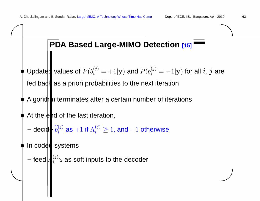
• Updated values of P (b(j)i = +1|y) and P (b
(j)i = −1|y) for all i, j are
fed back as a priori probabilities to the next iteration
• Algorithm terminates after a certain number of iterations
• At the end of the last iteration,
– decide b(j)i as +1 if Λ
(j)i ≥ 1, and −1 otherwise
• In coded systems
– feed Λ(j)i ’s as soft inputs to the decoder
A. Chockalingam and B. Sundar Rajan: Large-MIMO: A Technology Whose Time Has Come Dept. of ECE, IISc, Bangalore, April 2010 64'
&
$
%
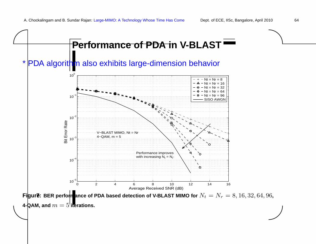
Performance of PDA in V-BLAST
* PDA algorithm also exhibits large-dimension behavior
0 2 4 6 8 10 12 14 1610
−5
10−4
10−3
10−2
10−1
100
Average Received SNR (dB)
Bit
Err
or R
ate
Nt = Nr = 8Nt = Nr = 16Nt = Nr = 32Nt = Nr = 64Nt = Nr = 96SISO AWGN
V−BLAST MIMO, Nt = Nr4−QAM, m = 5
Performance improveswith increasing Nt = Nr
.
Figure7: BER performance of PDA based detection of V-BLAST MIMO for Nt = Nr = 8, 16, 32, 64, 96,
4-QAM, and m = 5 iterations.
A. Chockalingam and B. Sundar Rajan: Large-MIMO: A Technology Whose Time Has Come Dept. of ECE, IISc, Bangalore, April 2010 65'
&
$
%
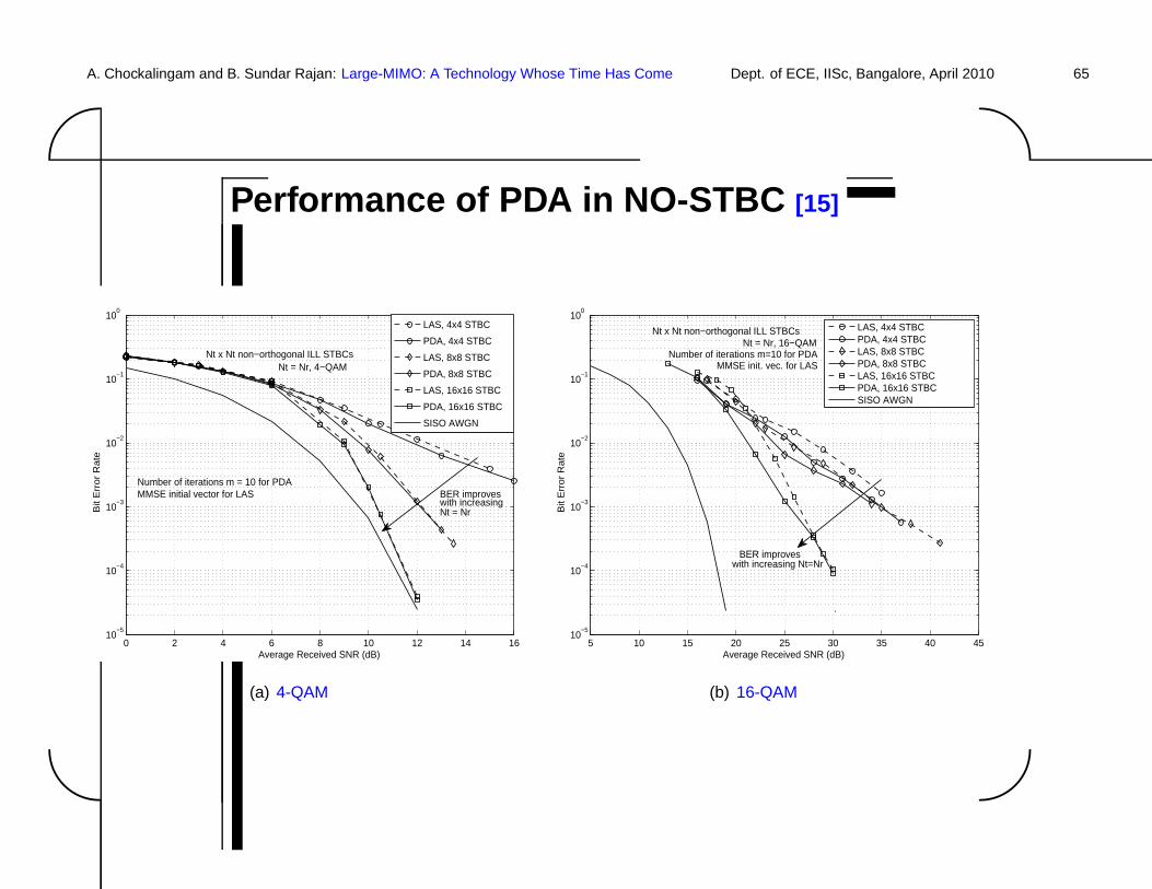
Performance of PDA in NO-STBC [15]
0 2 4 6 8 10 12 14 1610
−5
10−4
10−3
10−2
10−1
100
Average Received SNR (dB)
Bit
Err
or
Ra
te
LAS, 4x4 STBC
PDA, 4x4 STBC
LAS, 8x8 STBC
PDA, 8x8 STBC
LAS, 16x16 STBC
PDA, 16x16 STBC
SISO AWGN
BER improveswith increasingNt = Nr
Nt x Nt non−orthogonal ILL STBCsNt = Nr, 4−QAM
Number of iterations m = 10 for PDAMMSE initial vector for LAS
(a) 4-QAM
5 10 15 20 25 30 35 40 4510
−5
10−4
10−3
10−2
10−1
100
Average Received SNR (dB)
Bit
Err
or
Ra
te
LAS, 4x4 STBCPDA, 4x4 STBCLAS, 8x8 STBCPDA, 8x8 STBCLAS, 16x16 STBCPDA, 16x16 STBCSISO AWGN
Nt x Nt non−orthogonal ILL STBCsNt = Nr, 16−QAM
Number of iterations m=10 for PDAMMSE init. vec. for LAS
BER improves with increasing Nt=Nr
.
(b) 16-QAM
A. Chockalingam and B. Sundar Rajan: Large-MIMO: A Technology Whose Time Has Come Dept. of ECE, IISc, Bangalore, April 2010 66'
&
$
%
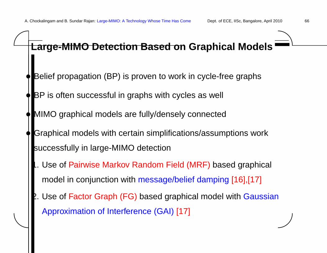
Large-MIMO Detection Based on Graphical Models
• Belief propagation (BP) is proven to work in cycle-free graphs
• BP is often successful in graphs with cycles as well
• MIMO graphical models are fully/densely connected
• Graphical models with certain simplifications/assumptions work
successfully in large-MIMO detection
1. Use of Pairwise Markov Random Field (MRF) based graphical
model in conjunction with message/belief damping [16],[17]
2. Use of Factor Graph (FG) based graphical model with Gaussian
Approximation of Interference (GAI) [17]
A. Chockalingam and B. Sundar Rajan: Large-MIMO: A Technology Whose Time Has Come Dept. of ECE, IISc, Bangalore, April 2010 67'
&
$
%
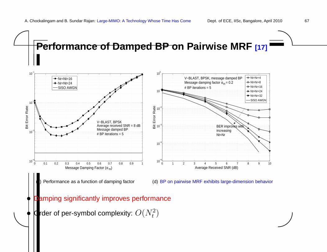
Performance of Damped BP on Pairwise MRF [17]
0 0.1 0.2 0.3 0.4 0.5 0.6 0.7 0.8 0.9 110
−4
10−3
10−2
10−1
Message Damping Factor (α m)
Bit
Err
or
Ra
te
Nr=Nt=16Nr=Nt=24SISO AWGN
V−BLAST, BPSK
# BP iterations = 5Message damped BP Average received SNR = 8 dB
(c) Performance as a function of damping factor
0 1 2 3 4 5 6 7 8 9 1010
−5
10−4
10−3
10−2
10−1
100
Average Received SNR (dB)
Bit
Err
or
Ra
te
Nt=Nr=4
Nt=Nr=8
Nt=Nr=16
Nt=Nr=24
Nt=Nr=32
SISO AWGN
V−BLAST, BPSK, message damped BPMessage damping factor α
m = 0.2# BP iterations = 5
BER improves withincreasingNt=Nr
(d) BP on pairwise MRF exhibits large-dimension behavior
• Damping significantly improves performance
• Order of per-symbol complexity: O(N2t )
A. Chockalingam and B. Sundar Rajan: Large-MIMO: A Technology Whose Time Has Come Dept. of ECE, IISc, Bangalore, April 2010 68'
&
$
%
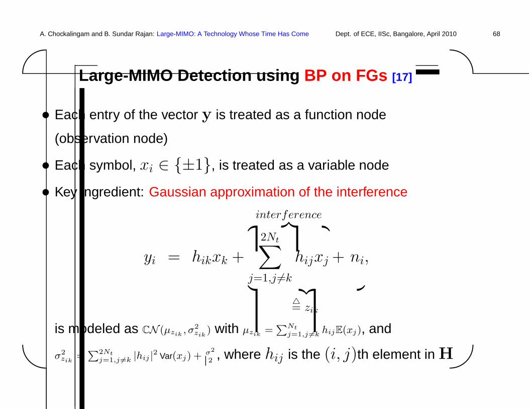
Large-MIMO Detection using BP on FGs [17]
• Each entry of the vector y is treated as a function node
(observation node)
• Each symbol, xi ∈ {±1}, is treated as a variable node
• Key ingredient: Gaussian approximation of the interference
yi = hikxk +
interference︷ ︸︸ ︷2Nt∑
j=1,j 6=k
hijxj + ni
︸ ︷︷ ︸△= zik
,
is modeled as CN (µzik, σ2
zik) with µzik
=PNt
j=1,j 6=khijE(xj), and
σ2zik
=P2Nt
j=1,j 6=k |hij |2 Var(xj) + σ2
2, where hij is the (i, j)th element in H
A. Chockalingam and B. Sundar Rajan: Large-MIMO: A Technology Whose Time Has Come Dept. of ECE, IISc, Bangalore, April 2010 69'
&
$
%
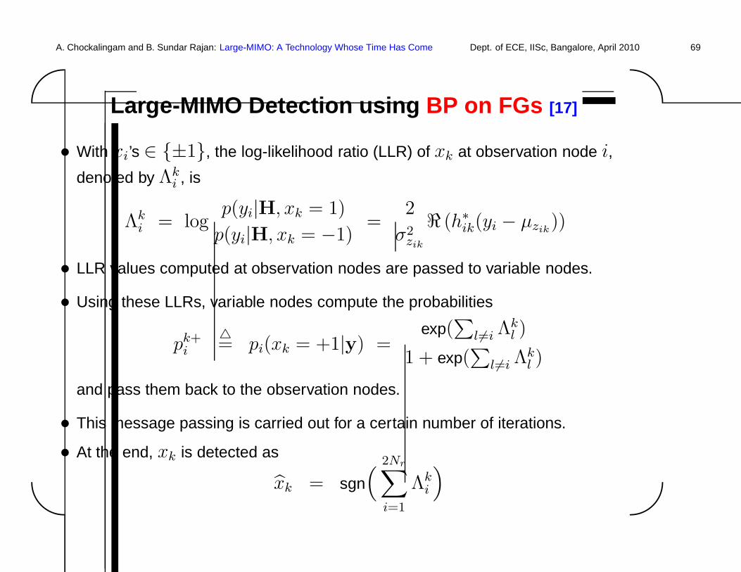
Large-MIMO Detection using BP on FGs [17]
• With xi’s ∈ {±1}, the log-likelihood ratio (LLR) of xk at observation node i,
denoted by Λki , is
Λki = log
p(yi|H, xk = 1)
p(yi|H, xk = −1)=
2
σ2zik
ℜ (h∗ik(yi − µzik
))
• LLR values computed at observation nodes are passed to variable nodes.
• Using these LLRs, variable nodes compute the probabilities
pk+i
△= pi(xk = +1|y) =
exp(∑
l 6=i Λkl )
1 + exp(∑
l 6=i Λkl )
and pass them back to the observation nodes.
• This message passing is carried out for a certain number of iterations.
• At the end, xk is detected as
xk = sgn( 2Nr∑
i=1
Λki
)
A. Chockalingam and B. Sundar Rajan: Large-MIMO: A Technology Whose Time Has Come Dept. of ECE, IISc, Bangalore, April 2010 70'
&
$
%
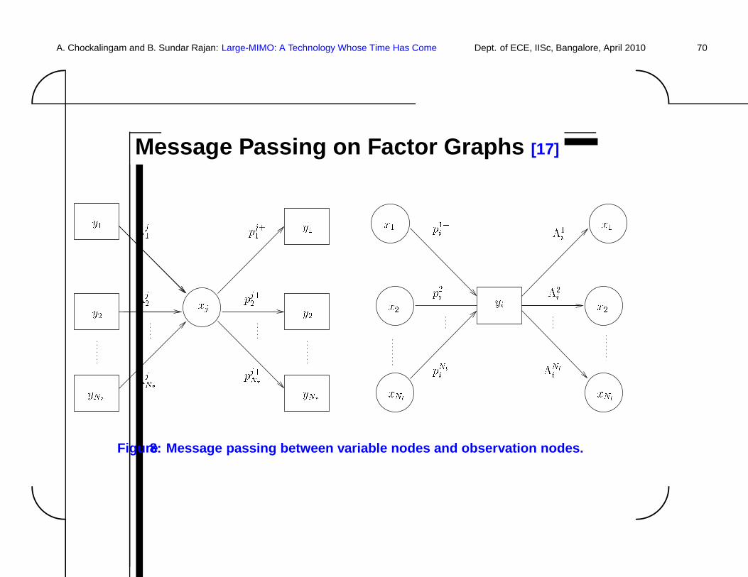
Message Passing on Factor Graphs [17]
y2yNr
y1y2
yNrxj
y1 �j1�j2
�jNrpj+1
pj+2pj+Nr
x1xNt
x1
x2 x2xNt
yip2+ip1+i
pNt+i �Nti�1i�2i
Figure8: Message passing between variable nodes and observ ation nodes.
A. Chockalingam and B. Sundar Rajan: Large-MIMO: A Technology Whose Time Has Come Dept. of ECE, IISc, Bangalore, April 2010 71'
&
$
%
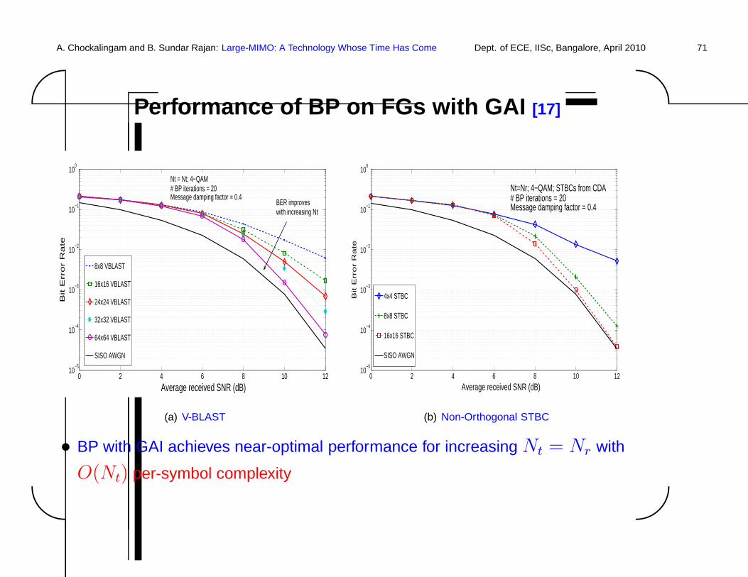
Performance of BP on FGs with GAI [17]
0 2 4 6 8 10 1210
−5
10−4
10−3
10−2
10−1
100
Average received SNR (dB)
Bit E
rro
r R
ate
8x8 VBLAST
16x16 VBLAST
24x24 VBLAST
32x32 VBLAST
64x64 VBLAST
SISO AWGN
BER improves with increasing Nt
Nt = Nt; 4−QAM# BP iterations = 20Message damping factor = 0.4
(a) V-BLAST
0 2 4 6 8 10 1210
−5
10−4
10−3
10−2
10−1
100
Average received SNR (dB)
Bit E
rro
r R
ate
4x4 STBC
8x8 STBC
16x16 STBC
SISO AWGN
Nt=Nr; 4−QAM; STBCs from CDA# BP iterations = 20Message damping factor = 0.4
(b) Non-Orthogonal STBC
• BP with GAI achieves near-optimal performance for increasing Nt = Nr with
O(Nt) per-symbol complexity
A. Chockalingam and B. Sundar Rajan: Large-MIMO: A Technology Whose Time Has Come Dept. of ECE, IISc, Bangalore, April 2010 72'
&
$
%
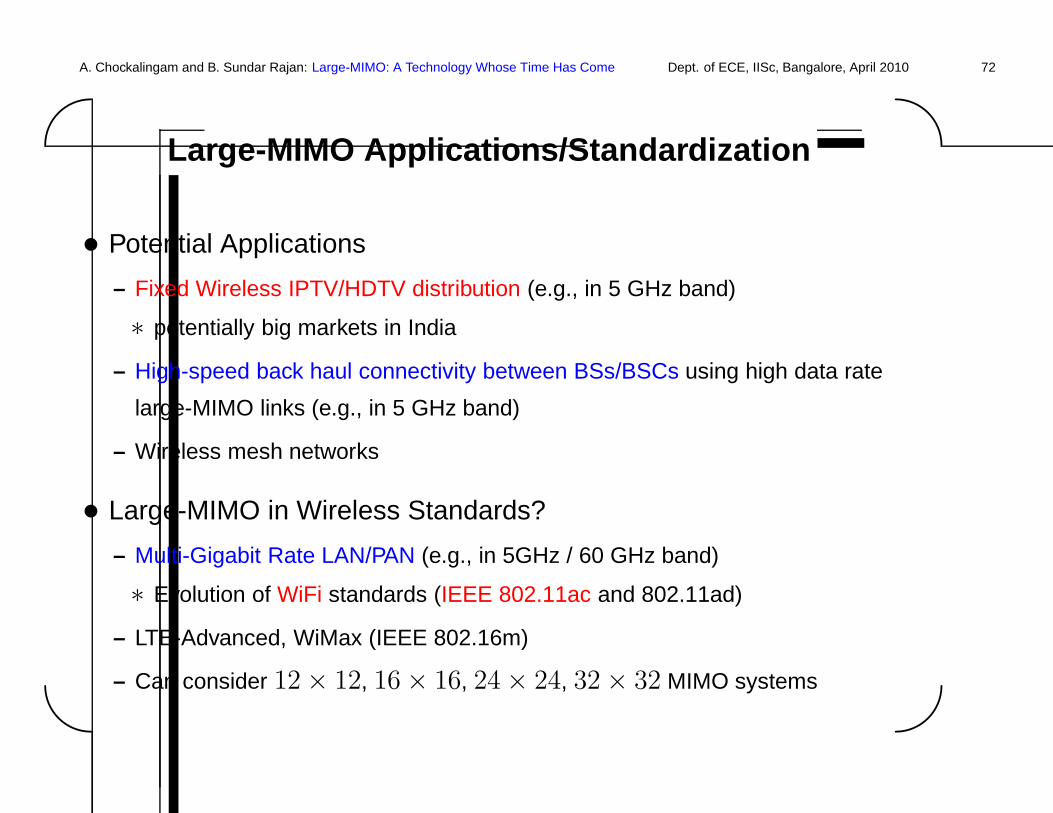
Large-MIMO Applications/Standardization
• Potential Applications
– Fixed Wireless IPTV/HDTV distribution (e.g., in 5 GHz band)
∗ potentially big markets in India
– High-speed back haul connectivity between BSs/BSCs using high data rate
large-MIMO links (e.g., in 5 GHz band)
– Wireless mesh networks
• Large-MIMO in Wireless Standards?
– Multi-Gigabit Rate LAN/PAN (e.g., in 5GHz / 60 GHz band)
∗ Evolution of WiFi standards (IEEE 802.11ac and 802.11ad)
– LTE-Advanced, WiMax (IEEE 802.16m)
– Can consider 12 × 12, 16 × 16, 24 × 24, 32 × 32 MIMO systems
A. Chockalingam and B. Sundar Rajan: Large-MIMO: A Technology Whose Time Has Come Dept. of ECE, IISc, Bangalore, April 2010 73'
&
$
%
Concluding Remarks
• Low-complexity detection
– critical enabling technology for large-MIMO
– no more a bottleneck
• Large-MIMO systems can be implemented
• Large-MIMO approach scores high on spectral efficiency and
operating SNR compared to other approaches (e.g., increasing
QAM size)
• Standardization efforts can consider reaping the benefits of
large-MIMO in their evolution
A. Chockalingam and B. Sundar Rajan: Large-MIMO: A Technology Whose Time Has Come Dept. of ECE, IISc, Bangalore, April 2010 74'
&
$
%
Thank You