A Bayesian approach to auto-calibration for parametric array signal processing

IEEE TRANSACTIONS ON SIGNAL PROCESSING, VOL. 42, NO. 12, DECEMBER 1YY4 3495

A Bayesian Approach to Auto-Calibration for Parametric Array Signal Processing

Mats Viberg, Member, IEEE, and A. Lee Swindlehurst, Member, IEEE

Abstract- A number of techniques for parametric (high- resolution) array signal processing have been proposed in the last few decades. With few exceptions, these algorithms require an exact characterization of the array, including knowledge of the sensor positions, sensor gaidphase response, mutual coupling, and receiver equipment effects. Unless all sensors are identical, this information must typically be obtained by experimental measurements (calibration). In practice, of course, all such information is inevitably subject to errors. Recently, several different methods have been proposed for alleviating the inherent sensitivity of parametric methods to such modeling errors. The technique proposed herein is related to the class of so-called auto-calibration procedures, but it is assumed that certain prior knowledge of the array response errors is available. This is a reasonable assumption in most applications, and it allows for more general perturbation models than does pure auto-calibration. The optimal maximum a posteriori (MAP) estimator for the problem at hand is formulated, and a computationally more attractive large-sample approximation is derived. The proposed technique is shown to be statistically efficient, and the achievable performance is illustrated by numerical evaluation and computer simulation.

I. INTRODUCTION

HE field of array signal processing is concerned with T the problem of extracting information from measurements taken by an array of spatially distributed sensors. This research area has received much attention over the last few decades, and many relevant parameter estimation methods have been proposed. These techniques find application in such diverse disciplines as radar detection, radio and satellite mmmunica- tion, underwater source localization, and seismic exploration. As the terminology implies, parametric techniques require access to a parametrized model of the array measurements.

The assumed data model includes the response of the array to emitters as a function of their spatial and temporal parameters, such as bearing, range, polarization, frequency, etc. Hence, the array geometry and the gaidphase characteristics of the sensors and the associated receiver equipment must be

Manuscript received June 12, 1993; revised May 25, 1994. This work was supported by the Advanced Research Projects Agency of the Department of Defense, monitored by the Air Force Office of Scientific Research under Grant No. F49620-91-C-0086; by the SDIO/IST Program, managed by the Army Research Office under Grant DAAH04-93-G-0029; and by the Na- tional Science Foundation under Grant MIP-9110112. The associate editor coordinating the review of this paper and approving it for publication was Prof. Daniel Fuhrmann.

M. Viberg is with the Department of Applied Electronics, Chalmers University of Technology, S-412 96 Gothenburg, Sweden.

A. Swindlehurst is with the Department of Electrical and Computer Engi- neering, Brigham Young University, Provo, UT 84602 USA.

IEEE Log Number 9406019.

known to the user. If this is not the case, or if, for exarrple, the sensors are subject to mutual coupling, the array must be calibrated. This is normally done by experimentally measuring the array response to sources at different locations. In either case, the assumed model is bound to differ from the actual response at the time of data collection. This may be due to time-varying environmental conditions, or simply to errors in the chosen model structure. The effects of such model errors have been studied by several authors, e.g., [1]-[6]. These effects can be contrasted with estimation errors induced by the necessity of collecting only a finite amount of data from the array, e.g., as studied in [7]-[13]. In many cases of practical interest, the effects of modeling errors have at least as great an influence on the total estimation error as do the finite sample effects of noise.

While most estimation algorithms have been developed with only finite sample effects in mind, alternative techniques that only take model errors into account have been proposed in [6] and [14]. An optimal approach to the problem must account for both sources of errors simultaneously. One idea would be to estimate the unknown parameters of the array response simultaneously with the signal parameters. Such techniques are referred to as auto-calibration methods, and have been proposed in, for example, [15]-[17]. An alternative is to view the modeling errors as random with known second-order statistics. Optimally weighted subspace fitting methods based on this model are derived in [6] and [ 141 (model errors only) and [ 181 and [ 191 (both model errors and finite sample effects).

One drawback associated with auto-calibration techniques is that, in many situations, the array response and signal location parameters are not independently identifiable. For instance, it is not possible to estimate both sensor phase characteristics and signal bearing angles. On the other hand, the techniques pursued in [6], [14], and [18] can only give optimal performance in special cases (as will be demonstrated in Section IV-C). Herein, we consider a combination of the two approaches. That is, the array perturbation parameters are assumed to be random with known a priori distribution, and are estimated in a Bayesian framework along with the signal parameters. Similar ideas have appeared, e.g., in [20]-[24], and the results of the latter reference are taken as a starting point for the present work.

One of the main contributions of this paper is the development of an algorithm that is computationally much simpler than the optimal maximum a posteriori (MAP) estimator, but is asymptotically equivalent in performance. The proposed

1053-587>094$04.00 0 1994 IEEE

Authorized licensed use limited to: IEEE Editors in Chief. Downloaded on August 17, 2009 at 19:23 from IEEE Xplore. Restrictions apply.

3496 IEEE TRANSACTIONS ON SIGNAL PROCESSING, VOL. 42. NO. 12. DECEMBER 1991

method combines the ideas of [24] and the noise subspace fitting (NSF) approach of [25], and hence is referred to as the MAP-NSF algorithm. Use of the NSF problem formulation decouples the estimation of the directions of arrival (DOA’s) of the signals and the array perturbation parameters, and yields a criterion function that depends only on the DOA’s. The array calibration parameters can then be solved for directly, if desired. In addition to developing the MAP-NSF algorithm and verifying its asymptotic efficiency, we also present a compact expression for the CramCr-Rao bound (CRB) for the case where both finite sample effects and model errors are present.

The remainder of the paper is organized as follows. In the next section, the data model is formulated along with some fundamental assumptions and results. Secti0.n I11 presents both the MAP and MAP-NSF estimators, and Section IV explores some connections between MAP-NSF and other existing approaches. The compact expression for the CRB is presented in Section V, and the statistical efficiency of MAP- NSF is established. The resulting expression for the asymptotic estimation error covariance is examined using some illustrative examples in Section VI, along with computer simulations to investigate the usefulness of the asymptotic expressions for performance prediction.

11. PROBLEM FORMULATION

This section introduces notation and briefly presents some preliminary results that are necessary for the analysis that follows.

A. Data Model

Consider an array of 7n sensors having arbitrary positions and characteristics. Impinging on the array are the waveforms of d narrowband point sources, where d < m. The vector of sensor outputs is denoted x ( t ) , and is modeled by the following familiar equation:

x(t) = [ 4 H 1 3 P ) I . . . l 4 H d , PI1 [;;?;;] + n(t)

= A ( B , p ) s ( t ) + n(t). (1)

The columns of the m x d matrix A are the so-called array propagation vectors, denoted U( H L , p ) . i = 1, . . . , d. These vectors describe the array response to a unit waveform with signal parameter(s) OL. The above model also allows for unknown “perturbation parameters,” collected in the real 71-

vector p = [ P I , . . . p1,IT. This includes structured parameters, such as sensor gain, phase, position, and/or mutual coupling, as well as unstructured parameters (see Section IV-C). The nominal array response is assumed to be unambiguous; i.e., the matrix [.(e,, po). . . . , a(H,,po)] has full rank for any collection of distinct parameters 01, . . . , Or, .

Though not necessary, it is assumed in our discussion that H , is a real scalar, referred to as the zth DOA. The components of the d-vector 0 are the DOA’s of the model, whereas the vector 00 represents their true values. It is further assumed that the array response parameters in p represent small de- viations from their known nominal values, collected in the

vector po. The a priori covariance matrix of the perturbation, denoted by C l , is also assumed known. This matrix could be determined, for example, using sample statistics from a number of independent, identical calibration experiments, or using tolerance data specified by the manufacturer of the sensors. The complex d-vector s ( t ) is composed of the emitter waveforms received at time t , and the m-vector n(t) accounts for additive measurement noise. The array output is assumed to be sampled at N distinct time instants. Based on these measurements, x(l) , . . . ~ x ( N ) , the problem of interest is to determine the DOA’s of all emitters. The number of signals, d, is assumed to be known.

Although the signal waveforms will be assumed to be Gaussian random processes when deriving the exact MAP estimator and the CRB, the properties of the proposed method will be analyzed under a less restrictive assumption. The signal waveforms are then regarded as arbitrary deterministic (i.e., fixed) sequences such that the following limit exists and is positive definite:

where { .}* denotes the complex conjugate transpose. Simi- larly, we assume that the perturbation parameters are drawn from a Gaussian distribution when deriving the MAP estimator and the CRB, although the Gaussian assumption is relaxed when analyzing the resulting estimator.

On the contrary, the noise term n(t) is modeled as a stationary, complex Gaussian random process, uncorrelated with the signals. The noise has zero mean and is assumed to be circularly symmetric as well as spatially and temporally white:

~ [ n ( t ) n * ( s ) ] = (T’I&,,~ ( 3 ) ~ [ n ( t ) n ~ ( s ) ] = o (4)

where dt., is the Kronecker delta. Since we are interested in studying the combined effects

of finite sample errors and modeling errors, the size of the perturbations relative to the number of available snapshots plays a crucial role. The variances of the estimated DOA’s are known to be proportional to 1/N in the finite-sample-only case, whereas they are proportional to Cl in the model-error- only case. In this analysis, the relative contribution of the two error sources will be assumed to be of comparable magnitude, and the covariance matrix of the perturbation parameters will be expressed as

where fi is independent of N . In Section V, a performance analysis is carried out assuming N to be “large enough.” An argument for the somewhat artificial assumption ( 5 ) is that if Cl = o(l/N), then the effect of the modeling errors can be neglected and the methods designed for finite sample errors only are optimal. On the other hand, if W1 = o ( N ) , the effect of the modeling errors dominates, thus rendering the methods designed solely for such errors optimal. Since the MAP approach presented herein is inherently more complicated than


VlBERG AND SWINDLEHLRST. A BAYESIAN APPROACH TO AUTO-CALIBRKTION 3497

either of the methods that take only finite samples or modeling errors into account, the former should be avoided when one type of error dominate\ the other.

B. Preliminary Results

In the next section, the exact MAP estimator is presented along with a less computationally demanding approximation. The proposed approximate technique is a subspace-based method, in that it relies heavily on the properties of the eigendecomposition of the array covariance. Under the above assumptions, the covariance matrix of the array output takes the form

1 N-x, N R = lim - E[x(t)x*(t)]

t=l

Since the matrix APA* has rank d by assumption (the arguments of A will frequently be suppressed for notational convenience), c? is an eigenvalue of R with multiplicity m-d, and the corresponding eigenvectors are all orthogonal to A. The eigendecomposition of R thus takes the form

IT1

R = X,,eie: = E,A,E: + a 2 ~ , , ~ , * , (7) /=1

where A, is a diagonal matrix containing the d largest eigen- values, and the columns of the 'rr1 x d matrix E, are the corresponding unit-norm eigenvectors. Similarly, the columns of E,, are the T u - d eigenvectors corresponding to 0'. Since E,, is orthogonal to A, it follows that the range space of E, coincides with that of A. This observation forms the basis for all subspace-based estimation techniques, starting with the development of the popular MUSIC algorithm [26], [27]. Assuming orthonormal eigenvectors, the orthogonal projection onto the range space of A is denoted

n = A(A*A)-IA* = E,sEZ (8)

and its orthogonal complement is

nL = I - A ( A * A ) - ~ A * = E,,E;. (9)

We now derive some expressions for the signal covariance matrix that will be useful in the subsequent analysis. Combining (6) and (7) we get

APA* = E,AE: (10)

where

Denoting the pseudo-inverse of A by

(10) implies

P = A+E,JE,*A+*. (13)

Noting that (AtE,)-' = EZA, the inverse of the above equation can be written as

p - l = A*E,A-~E;A. (14)

Under the stated assumptions, the eigendecomposition of R can be consistently estimated by performing an eigendecomposition of the sample covariance matrix

N R='C x(t)x*(t) = EsAsE: + EnAnEz (15) t=l

N

where the partitioning of the eigen-elements is similar to (7).

111. ROBUST ESTIMATION

In this section, the exact MAP formulation of the problem is presented, along with a simplified but asymptotically equivalent approximation.

A. Exact MAP Estimation

When deriving the MAP estimator, it will be assumed that the a priori distribution of p is Gaussian with known mean po and covariance matrix SI. Likewise, the emitter signals, s ( t ) are modeled as zero-mean Gaussian with second-order moments

E [ S ( t ) S * (s)] = Pbt,, (16)

E[s(t)sT(s)] = 0. (17)

The signal parameters, 8, the emitter covariance, P, and the noise variance, U', are all regarded as unknown deterministic parameters (i.e., parameters with a non-informative a priori distribution). Following [24], the joint MAP estimate of 8, P, o2 and p is then obtained as

{e, b, P, 2 1 = arg niin vnIAP(e. p, P, 2) (18) ~ , P F P '

when SI is full rank. Here, VhfL(8.p%P,a2) is the negative log-likelihood function, which is given by [28]

k ( e , p , P , n2) = N ( h g IR(8. p, P, g2)1

+ Tr{R-l(8. p3 P , 02)R}) + const.

(20)

where I . I denotes the determinant. The ML criterion function is known to be separable in P and 0'. For fixed A = A(8. p ) , the minimizing signal covariance matrix and noise power are [281

p = At(& - eZI)Af*

Tr{ nL R} . 1 6 2 = -

m - d

Substituting (21)-(22) into (20) leads to [29]

vhlL(o,p) = mog IAPA* + 6211 t


1498

Clearly, Vbr.kp(B.p,P,c2) is also separable in P and a’, and ignoring constant terms the concentrated MAP criterion function is

1 V , , , ~ ( ~ , P ) = vklL(e,p) + ,(P - P , , ) ~ s ~ - ’ ( P -pa). (24)

This can be interpreted as a regularized ML criterion. That is, the effect of the prior distribution is to force i, to be close to the nominal value, po. If the perturbation parameters are identifiable, this effect is diminished as the number of snapshots N increases. Thus, the MAP estimate has the same asymptotic properties as the ML estimate (i.e., the pure auto-calibration technique). However, in many applications of interest, p cannot be consistently estimated along with the signal parameters. In such cases the prior distribution has a crucial influence on the asymptotic properties of the estimates of both B and p.

IEEE TRANSACTIONS ON SIGNAL PROCESSING, VOL. 42, NO. 12. DECEMBER 1994

B. The MAP-NSF Method

It has been assumed that the signal covariance matrix has full rank; i.e., the signals are noncoherent. Then it is known [29] that in the absence of model errors, the ML criterion is asymptotically equivalent to the following noise subspace fitting (NSF) criterion

V&F = NTr{A*E:,EiAU} (25)

where U denotes a consistent estimate of the matrix

U = a - 2 ~ + ~ , h 2 ~ ; 1 ~ ; ~ + * = o - 2 ~ ~ * ~ - 1 ~ ~ . (26)

In the present case, the term “asymptotic equivalence” is to be interpreted as

Here q refers to any component of B or p, and the symbol o , ( l / f i ) represents a term that tends to zero faster than l/Jl?i in probability. The extension of this result to the case where model errors are also present is immediate since the proof only depends on the fact that R = R + O,( l / f l ) . By standard first-order arguments, this implies that the MAP estimate is asymptotically (for large N ) equivalent to the minimizing arguments of the criterion function

(28) 1

h S F ( B . p ) + 5 ( p - p o ) T f i 2 - 1 ( P - Po) .

This criterion depends on its parameters in a simpler way than the exact MAP criterion (24). However, it still requires a nonlinear minimization over both B and p.

Making use of the assumption that S1 decreases as 1/N, a further simplification of the criterion is possible that enables separation with respect to p. Recall the following formulas for the vet(.) operator (vectorization of a matrix by stacking its columns) and the Kronecker product @ (see [30], [311)

Tr{ABCD} = vec(D7)‘(CT @ A)vec(B) (29) (30) (31) (32)

vec(ABC) = (C’ @ A)vec(B)

(A 8 B ) ( C @ D) = ( (AC) @ (BD)) (A B B)’ = A~ R B ~ .

Using (29), the NSF criterion can be rewritten as

NTr{A*EnE:AU} = Na*Ma (33)

where

a = vec(A) (34) M = UT @ (Er,EZ). ( 3 5 )

Next, the vectorized steering matrix is approximated locally around po as

a = a(B, p ) = a0 + Dp+ (36)

where

P = P - Po. (39)

Note that, when evaluated at po, the derivative of a with respect to B or p is identical to that of a0 + Dp+. It follows that the minimizing arguments of (33) are asymptotically identical to the estimates obtained by minimizing the following approximate MAP-NSF criterion with respect to B and p :

1-7 - -1- (a0 + D,+)*M(ao + D,j) + 2~ P (40)

Since the criterion function in (40) is quadratic in p , we

(41)

where we have normalized by N and used (5).

easily obtain the minimum with respect to fi (for fixed 0) as

bMAP-NSF = PO - r-lf

where

(42) 2

f = Re{D;Mao}. (43)

Substituting (41) into (40) leads to the following separated criterion function

a;Mao - Pr-9. (44)

Note that I’ and f depend on 8 through D,, and in principle M also depends on 8 through U. However, it will be assumed that a consistent estimate of B is available to form the estimates M, f and r. Under the stated assumptions, such an, estimate can be obtained, for instance, by letting p = po and U = I in (25), which leads to the well known MUSIC algorithm (see [25]&fof details). As will be seen later, the approximations made in r, f and M do not change the asymptotic properties of the final estimate. The definitions of the quantities in the MAP-NSF cost function are repeated below for easy reference, followed by a summary of the proposed algorithm:

a0 = vec(A(B. Po) ) (45) M = 6-2(A+Es(As - 2 1 ) 2 A ; l E ; A + * ) T @ (EnE;J

(46)

Tr{ (I - AAt)R} 1

8 2 = - 111 - d (47)


VIBEKG AND SWINDLEHURST A BAYESIAN APPROACH TO AUTO-CALIBRATION 3499

(48) an arbitrary value. This results in the concentrated approximate criterion function

The MAP-NSF Algorithm: Given the sample covariance R x [ a p p v W S F f fl-’]-’apV\VSF (54) and an initial estimate e of the DOA’s:

a) Compute the eigendecomposition R = EsAsE; + b) Compute the quantities (46)-(48) c) Using 8 as an initial guess, use a numerical method to

EnAnE;t

solve the following optimization problem

Iv . RELATIONSHIP TO OTHER TECHNIQUES

This section presents some connections between the proposed MAP-NSF method and existing techniques for DOA estimation under model uncertainties.

A. Autocalibration

Autocalibration usually refers to techniques that simultaneously estimate the DOA’s and sensor positions. For most geometries, this is possible if the location of one sensor and the direction to another is known [20]. Herein, we consider a more general model where the array response depends on both the DOA’s as well as an arbitrary set of perturbation parameters. By assuming an a priari distribution for the perturbation parameters, these need not be identifiable from the data only, hence allowing for more flexible models. If the perturbation parameters are indeed identifiable, one may delete the influence of the prior by letting a-’ = 0 in (48). Thus, maximum likelihood autocalibration is a special case of the MAP approach considered herein. However, it should be noted that [17] uses a deterministic signal model as opposed to the stochastic Gaussian signal model assumed here. It is known that the stochastic signal model leads to superior performance regardless of the actual signal distribution, at least in the absence of model errors [111, I 131.

B. The MAPprox Approach

The MAPprox (MAP approximation) method is proposed in [24] as an alternative approximation of the exact MAP estimator. The method is derived in two steps. First, V&,(8, p) in (24) is replaced by the asymptotically equivalent signal subspace fitting criterion,

N (52) I/\\~SF = FTr{n’E,W\vs,B:}

W\\‘SF = (A7 - (T21)2AL1.

where

(53)

Second, an implicit Newton-step over p is performed, starting at the nominal value, po. The DOA parameter is kept fixed at

where dpVLtTSF denotes the gradient of V ~ S F with respect to p , evaluated at po and 8. Similarly, d p P V ~ ~ s ~ denotes the ‘‘p comer” of the Hessian matrix. In practice, the Gauss-Newton Hessian (see [32]) is used to avoid taking second derivatives. The MAP-NSF technique can also be derived by essentially following the above steps, but using the NSF criterion (25) in lieu of (52). It is conceivable that the two approaches are asymptotically equivalent when P > 0 (although this remains to be formally proved). The asymptotic equivalence of the methods is also indicated by the simulation examples in Section VI, where it is also observed that the MAPprox method appears to have better finite sample properties. The following important differences between the approaches should be noted:

The MAP-NSF method is only applicable if the signal covariance matrix is nonsingular. The MAP-NSF method allows “more approximations” of the criterion function without losing asymptotic efficiency. In particular, d, ,v~\~s~ in (54) cannot be replaced by a consistent estimate (see Section V-B).

This latter fact is the reason why MAP-NSF is preferred herein. It implies that the MAP-NSF criterion depends on 8 in a simpler way than does the MAPprox criterion, which considerably simplifies both the analysis and the implementation.

C. Signal Subspace Fitting

model for the perturbed array response: For the moment, consider the following simple unstructured

(55) A(8: p ) = A(8) + A where we define

Re { vec( A)} p = [Imivecc A)]]

and where the columns of A, denoted a,, are modeled as random variables with moments

E[a,]=O i = l , . . . , d (57) E[(LY6;] = V , k I Z. k = 1.. . . , d ( 5 8 ) E[6,iiT] = 0 (59) i , k = 1,. . . , d.

This model corresponds to an additive, circularly symmetric complex array perturbation that is uncorrelated from sensor to sensor, but possibly &dependent. It is easy to verify that under these assumptions, the covariance of p is given by

-Im{Y}@I

where the ‘1, kth element of the matrix r is U&. In [18] and [19], an “optimal” signal subspace fitting

algorithm is derived that takes into account both finite sample effects and the above array perturbation model. The algorithm


3500 IEEE TRANSACTIONS ON SIGNAL PROCESSING, VOL. 42, NO. 12. DECEMBER 1994

involves minimizing a criterion function identical to (52), but using the weighting matrix

-1

WosF = (E;A'.r'A'E, + -(As 8 2 - CP1)-2As) N

(61) in place of WWSF. Note that WOSF is just a weighted combination of WWSF, the optimal weighting when finite sample effects alone are considered, and the optimal weighting derived in [6] for the unstructured error model above when N -+ CO. The use of the term "optimal" here means that asymptotically, no other weighting matrix in (52) will yield DOA estimates with lower variance. We will now show that using WOSF in (52) yields an algorithm that is in fact asymptotically equivalent to MAP-NSF for the array perturbation model described above. Since the MAP-NSF method is asymptotically efficient (see Section V-C), no algorithm, whether or not it is in the form of (52), will yield asymptotically unbiased estimates with lower variance than the minimizing arguments of

Finally, we have

where

Using arguments similar to those in [29], it can be shown that the two cost functions

T~ begin with, note that in this case, = [I j ~ l . some simple algebra then yields (63), at the bottom of this page,

are asymptotically equivalent for any weighting matrix W , as long as the emitter covariance has rank. Thus,

we can conclude that MAP-NSF and OSF are asymptotically equivalent as well. When both algorithms are applicable, it is

since OSF is computationally less demanding and can handle

where we have used the fact that, for any invertible matrix X , for the simp1e perturbation described by (55)-(59),

Im{X-l} Re{X-l} '

(64) coherent emitters. 1 Re{X} -Imixr] - - [Reix-" -lm{x-l} preferable to use the OSF rather than the MAP-NSF criterion,

Multiplying out all terms in (63) and collecting real and imaginary parts leads to the simpler expression

Using the definition of M and an obvious notation, write M = UT c3 (E,Ei), and note that

l ) (M + ;Y-l @I) = ( ( U T + FY-l @ (EnE:)

-1

) -l 1 N

+ -Y-I c3 (EsE;)

-1

= (U' + ..Y-') 1 (EnE;)

V. ASYMPTOTIC PERFORMANCE ANALYSIS

In this section, the asymptotic properties of the proposed approximate MAP-NSF method are investigated. However, let us start the discussion by presenting an approximate bound on the achievable performance.

A. Crame'r-Rao Bound

The Cram&-Rao bound (CRB) gives a lower bound on the (asymptotic) covariance matrix of any (asymptotically) unbiased estimator. In the present case, the full parameter set contains both the deterministic parameters B , P, o', and the stochastic parameter p. We will collectively denote the deterministic parameters by the vector q. The CRB on q and p is the inverse of the Fisher information matrix (FIM) J. Assuming Gaussian signals and perturbation parameters, we have from [33] that J = J1 + Jz, where the i j th element of

f T t - l f = [Re{Mao}T Im{Mao}T1


VIBERG AND SWINDLEHURST A BAYESIAN APPROACH TO AUTO-CALIBRATION 3501

each term is given by

where Oi denotes the ,ith element of the compound parameter vector [$p”] T . Unfortunately, J1 is not easily evaluated. The p-parameter generally enters in a nonlinear fashion, rendering the expectation with respect to p difficult to compute. The exact expression has been computed in [20] for some special cases involving only a single emitter. However, a more com- mon approach is to ignore the expectation with respect to p, and evaluate J1 at po [22]. Following [24] and using (3, it can be shown that this approximation is of order O(1). Since J1 = O ( N ) , we will thus obtain an asymptotically valid CRB. The following “compact CRB” formula involving B and p only is given in [24] and*is restated herein for completeness:

Theorem I : Let 8 and 3, be asymptotically unbiased estimates of Bo and po, and assume that s ( t ) and p are Gaussian distributed. Then for large N we have

P - Po [“-“Ii P - Po 2 CRB (73)

where the i j th element of CRB-l is given by

2N CRB-l %.I = -RRe[Tr{AfIILAJ $

x PA* R- AP }I + fl G 1 U [ i , j ) . (74)

Here, A; denotes the derivative of A with respect to the ith

component of BTpT , and , U ( . , .) is an indicator function such that u ( l , j ) = 0 if either i 5 d or j 5 d j and u ( i , j ) = 1 otherwise. All expressions are evaluated at the true parameter values Bo and po.

To obtain a compact expression for the CRB on 0 only, introduce the notation

[ I T

(75)

FB = Re{DiMDo} (76) C = Re{DzMD8} (77)

where the matrices are evaluated at the “true” values, &,,Po. Then we have the following result:

Let 8 be an asymptotically unbiased estimate of Bo, and assume that s ( t ) and p are Gaussian distributed. Then, for large N the following inequality holds:

Corollary I :

1 2N

E[(8 - B , ) ( 8 - e,)”] 2 CRBg = - [C - Fir-’FO]-’

(78)

Proo) Straightforward from (74). 0 Note that, as derived in [ l l ] and [13], the asymptotic CRB

on B in the absence of modeling errors is given by Cp1/(2lv). We thus confirm the intuitively clear result that modeling errors can only deteriorate the attainable estimation accuracy. As will be seen later in this section, the proposed MAP-NSF

method attains the bound given in (78) regardless of the actual distribution of s ( t ) and p (although the right hand side of (78) is a lower bound on the attainable estimation error variance only for Gaussian signals and perturbations).

B. Consistency

Let us first verify that the MAP-NSF estimates converge with probability 1 (w.p.1) to the true values as ,N -+ CO. This holds true for any choice of weighting matrix U > 0, and for any value of 8 used in forming A and D,. To see this, note that the criterion function (5 1) is the Schur complement of the following matrix

(79)

Clearly, this matrix is positive definite if acMao > 0, and singular otherwise. lhus, we have V(B) 2 0, with equality iff Ma, = 0. Let M denote the limiting (as N i E) value of M. Then

Mao = (U’ @ (E,,E*,))vec(A(B, Po))

= vec(IILA(B, p,)U) (80)

where we have used (30) and the fact that E,EZ = I I l . Since the array is assumed to be unambiguous, Mao = 0 iff B = Bo. The convergence of the criterion function is uniform in B if the derivative of a0 is bounded, and it follows that the minimizing argument of (51) converges to Bo w.p.1 as N

It is interesting to note !hat any consistent estimate of 8 can be used in forming M in (79), without affecting the consistency of the final MAP-NSF estimate. As we will see later, this replacement does not even affect the asymptotic distribution of the estimate. One might be tempted to guess that it would similarly be possible to insert a consistent estimate of B into the Hessian matrix ~,,V&F, appearing in the MAPprox criterion function (54). However, the resulting criterion function then generally becomes unbounded from below, and consistency of the estimates cannot be guaranteed. Since dppVm~:s~ is usually a complicated function of 0, so is (54); therefore (5 1) results in a computationally simpler method.

oc.

C. Asymptotic Distribution

Although the estimates were shown to be consistent for arbitrary weighting matrices, their asymptotic properties are certainly affected by the weighting used. In the following, it is assumed that the optimal weightings (46)-(48) are used, and that the estimates of, these quantities are consistent, i.e., M -+ M, f’ + I’ and f --+ f (in probability) as N .+ ocj.

Since 8n;rApP.hrsF is consistent, a standard Taylor series expansion of the gradient of the criterion function around the estimate can be performed. This yields

(81)

where e = &,,~AP-NSF - 8 0 denotes the estimation error, V’ is the gradient of V(8) , and H is the asymptotic Hessian. Both V’ and H are evaluated at the true value Bo.

e = -H-’V’ + o p ( l / J N )


3502 IEEE TRANSACTIONS ON SIGNAL PROCESSING, VOL. 42. NO. 12. DECEMBER 1994

Consider first the derivative of (51) with respect to B i ,

denoted V,:

V , = 2Re{aiMai} - 2fTe-’ti

= 2Re{aZ;Myi} (82)

where y is defined by

j r = a. - D,,r-’f (83)

and its derivative with respect to Bi is n n A

(84) y . - a. - D r-lfi where denotes the derivative of 1 with respect to B i . Observe that EnE: = IIL + O,( l / f l ) , so that a{M = O , ( l / f l ) for any value of U (see (80)). Therefore, U, f and f can be replaced by their limiting values, denoted U , I’, and f respectively, without affecting the asymptotic (second-order) properties of Vi. The corresponding limiting yi is denoted yi . Thus,

( 8 5 )

Note that the only stochastic term in (85) is the EnE: term of M. To approximate this term we write

2 - 2 p

V, = 2Re{a;Myi} + o,(l/v%).

Ma0 ‘v vec(8,E;AU) (86)

where the arguments of a = a(O0,po) have been suppressed for notational convenience. The calculations in Appendix A show that

E T L E ; ~ 21 -II~RE,A-’E;A. (87)

By the central limit theorem (see e.g., Lemma 9.A.2 of [34]), R = R + O,(l/m) is asymptotically (for large N ) Gauss- ian distributed, and it follows from (81) and (85)-(87) that also the normalized estimation error has a limiting Gaussian distribution

f i e E ASJV(O,H-~QH-~) (88)

where Q is the asymptotic covariance matrix of the normalized gradient

Q = lirn N E [ v ’ v ’ ~ ] . (89)

Let e be the minimizing argument of the MAP- NSF cost function (51). Then e + 8, as N + 00. and the limiting distribution of the normalized estimation error is

(90)

where CRBo is the asymptotic CRB given by (78). ProoJ We need to verify that H = Q = ( N C R B @ ) - l .

However, these calculations are deferred to Appendix B. U As expected from the fact that the MAP-NSF method is

derived by first-order approximations to the optimal MAP estimator, the former (and hence also the latter) yields asymptotically efficient estimates. Recall that the interpretation of this result is that 8 is a minimum variance estimate when both N is “large enough” and 0 is “small enough”. The requirements on N and 0 for the estimates to be “practically efficient” may be quite demanding in difficult scenarios, as will be seen in the next section.

‘V-m

We thus have the following result: Theorem 2:

JN(e - e,) E A ~ N ( O , N C R B ~ )

D. Performance Without Auto- Calibration

It is of course of interest to assess the relative improvement offered by the auto-calibration technique as compared to techniques that do not exploit the perturbation model. We choose to compare with the WSF estimates [12], obtained by minimizing ( 5 2 ) with respect to 8. This method is known to be asymptotically equivalent with the stochastic maximum likelihood technique [28] and also with the NSF method (25)-(26) for the case P > 0. Thus, the following result applies to these other techniques as well.

Theorem 3: Let Bwsr be the minimizer of (52). Then

JN(eLl;sr - e,) E A ~ ( o : cwsF)

+ C - ~ F , ” ~ ~ F ~ C - ~ )

(91)

where

(92) c , ~ ’ ~ ~ = z(c-l 1

and where FB and C are defined in (76) and (77). Prooj? This result is a straightforward extension of The-

n Since the WSF method gives asymptotically unbiased es-

timates under the model considered herein, the Cramer-Rao inequality implies that CWSF 2 NCRBo. The difference between the two depends, of course, on the scenario. How- ever, note that for identifiable perturbation models (i.e., when D;MD, > 0), the “efficiency ratio” C \ \ ~ ~ F , ; ; / ( N C R B ~ , ~ ~ ) may be arbitrarily large for large N , since we then have CRBo + 0 as N + cc for a fixed value of 0, but C l v s ~ / N does not tend to zero unless C! -+ 0 as N + sm. In the more interesting case of unidentifiable perturbation parameters (D;MD, singular), the performance improvement offered by the MAP approach over WSF and other “conventional” DOA estimators may be less dramatic. An example is provided in the next section.

orem 1 in [19], and the proof is therefore omitted.

VI. SIMULATION EXAMPLES

In this section we study the performance of the MAP- NSF method in finite samples and under “moderately sized” perturbations. A comparison with the MAPprox and WSF methods is also included. As an application of the general perturbation model considered herein, we study a model suitable for arrays mounted on a flexible structure. The array is assumed to be planar, although an extension to the 3-D case is straightforward. It is assumed that the distances between the sensors is known and fixed. For simplicity, we approximate the flexible structure using a piecewise linear model, as illustrated in Fig. 1. This approximation is reasonable for small perturbations, which is the case of interest herein. The nominal array is assumed to be a uniform linear array (ULA) of m = 10 sensors, oriented along the x-axis of a coordinate system with its origin at the first sensor. The interelement spacing (T in the figure) is fixed at a half wavelength. In many cases of practical interest, there may be physical constraints that relate the incremental angles, thus leading to a perturbation model with fewer parameters (for example a polynomial model). However, here we assume that pz. i = 1, . . . . rri - 1. are independent zero-mean Gaussian random variables with variance U*, so


VlBEKG AND SWINDLEHURST: A BAYESlAN APPKOACH 'TO AUTO-CALLBKATION 3503

- 0 0 . . . 0- 1 0 . . . 0

x 2 1 (97) . . . . . .

- ' r r~ - 1 'rri - 2 . . . 1 -

fY I ,e

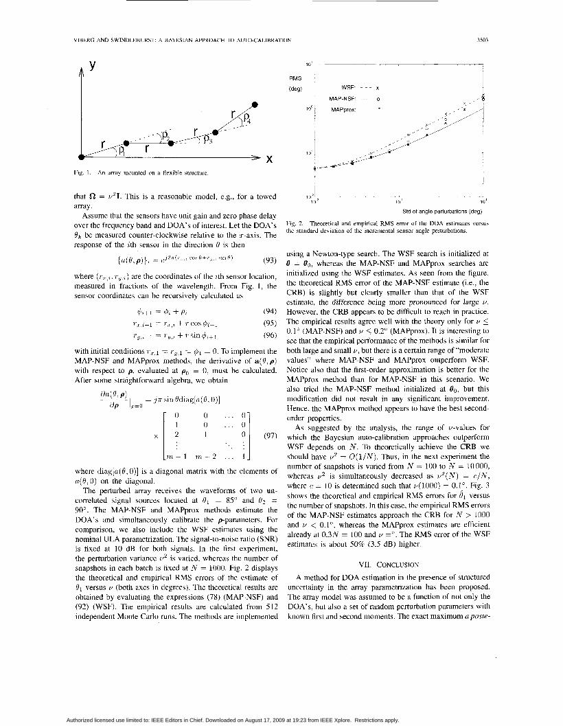
Fig. I . An array mounted on a flexible structure

that 51 = v21. This is a reasonable model, e.g., for a towed array.

Assume that the sensors have unit gain and zero phase delay over the frequency band and DOA's of interest. Let the DOA's el; be measured counter-clockwise relative to the x-axis. The response of the ith sensor in the direction 6' is then

(93)

where ( ~ , , i . r y . i ) are the coordinates of the ,ith sensor location, measured in fractions of the wavelength. From Fig. 1, the sensor coordinates can be recursively calculated as

{ u ( ~ , p ) \ - c:j2r(rL , (-oh O t r , >in 0) 1 -

4 r + l = 4 L + P i (94) (95) (96)

with initial conditions rZ.1 = ru:l = q+ = 0. To implement the MAP-NSF and MAPprox methods, the derivative of a(H, p) with respect to p, evaluated at po = 0, must be calculated. After some straightforward algebra, we obtain

7' , , j+l = Tx,z + T c:os @l+l

1 ' ,~ ,~+1 = r g , i + Tsin+i+l

l o ' , i

WSF: - - - x

MAP-NSF: - o 1 oo

l o ' :

MAPprox:

1 0 2 1 I l o 2 10 ' 1 on

Std of angle perturbations (deg)

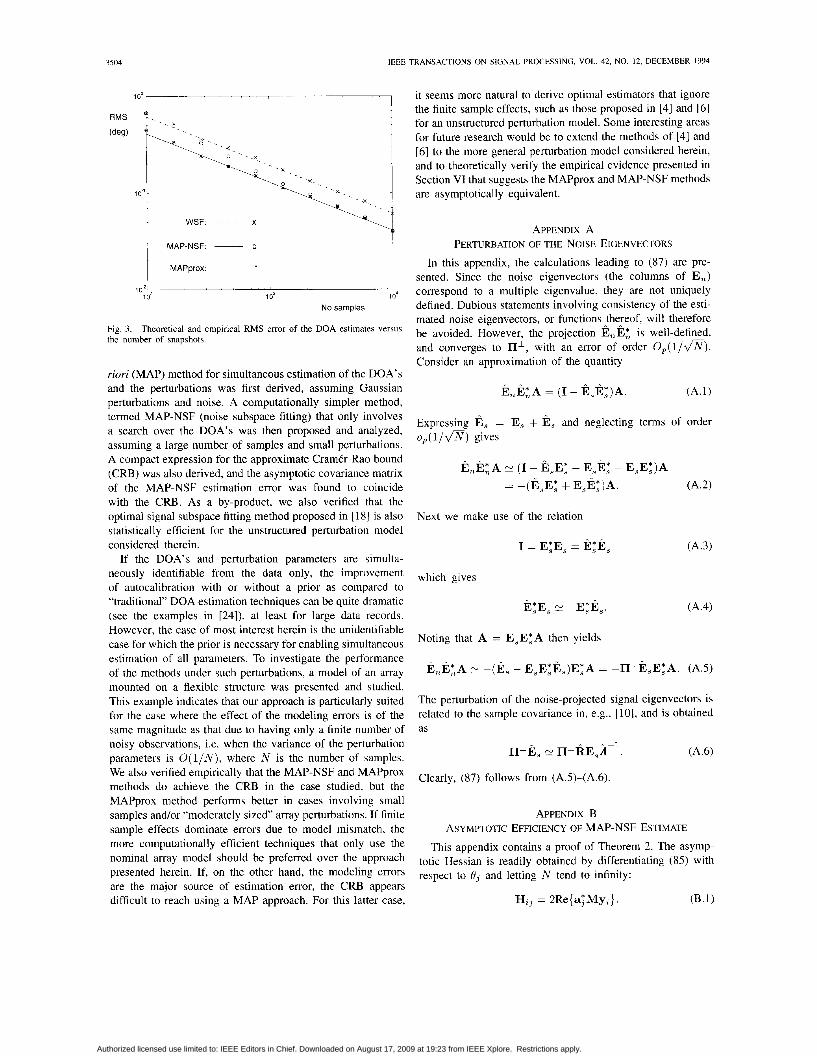
Fig. 2. the standard deviation of the incremental sensor angle perturbations.

Theoretical and empirical RMS error of the DOA estimates versus

using a Newton-type search. The WSF search is initialized at B = Bo, whereas the MAP-NSF and MAPprox searches are initialized using the WSF estimates. As seen from the figure, the theoretical RMS error of the MAP-NSF estimate (i.e., the CRB) is slightly but clearly smaller than that of the WSF estimate, the difference being more pronounced for large U .

However, the CRB appears to be difficult to reach in practice. The empirical results agree well with the theory only for v 5 0.1 " (MAP-NSF) and v 5 0.2" (MAPprox). It is interesting to see that the empirical performance of the methods is similar for both large and small v, but there is a certain range of "moderate values" where MAP-NSF and MAPprox outperform WSF. Notice also that the first-order approximation is better for the MAPprox method than for MAP-NSF in this scenario. We also tried the MAP-NSF method initialized at Bo, but this modification did not result in any significant improvement. Hence, the MAPprox method appears to have the best second- order properties.

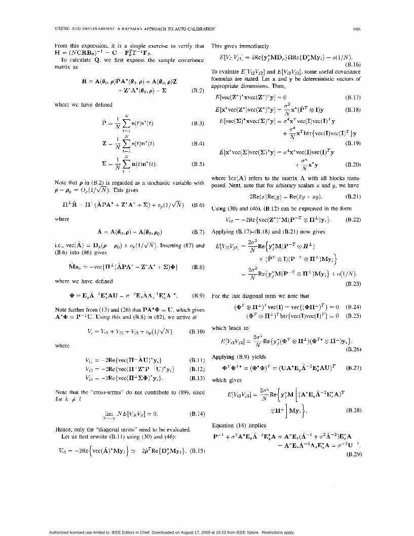
As suggested by the analysis, the range of v-values for which the Bayesian auto-calibration approaches outperform WSF depends on N . To theoretically achieve the CRB we should have v 2 = 0(1/N). Thus, in the next experiment the number of snapshots is vaned from N = 100 to N = 10000, whereas v 2 is simultaneously decreased as v 2 ( N ) = c / N , where c = 10 is determined such that ~ ( 1 0 0 0 ) = 0.1". Fig. 3 shows the theoretical and empirical RMS errors for 8, versus the number of snapshots. In this case, the empirical RMS errors of the MAP-NSF estimates approach the CRB for N > 1000 and v < 0.1", whereas the MAPprox estimates are efficient already at 0.3N = 100 and v =". The RMS error of the WSF estimates is about 50% (3.5 dB) higher.

VII. CONCLUStON

A method for DOA estimation in the presence of structured uncertainty in the array parametrization has been proposed. The array model was assumed to be a function of not only the DOA's, but also a set of random perturbation parameters with known first and second moments. The exact maximum aposfe-


3504 IEEE TRANSACTIONS ON SIGNAL PROCESSING, VOL. 42. NO. 12, DECEMBER 1994

RMS

(deg)

I O 0 ; I 1 1

x ’----; , , , , , I . MAP-NSF: ~ O

MAPprox:

1 o-2 1 o2 1 o3 i o 4

No samples

Fig. 3. the number of snapshots.

Theoretical and empirical RMS error of the DOA estimates versus

riori (MAP) method for simultaneous estimation of the DOA’s and the perturbations was first derived, assuming Gaussian perturbations and noise. A computationally simpler method, termed MAP-NSF (noise subspace fitting) that only involves a search over the DOA’s was then proposed and analyzed, assuming a large number of samples and small perturbations. A compact expression for the approximate CramCr-Rao bound (CRB) was also derived, and the asymptotic covariance matrix of the MAP-NSF estimation error was found to coincide with the CRB. As a by-product, we also verified that the optimal signal subspace fitting method proposed in [ 181 is also statistically efficient for the unstructured perturbation model considered therein.

If the DOA’s and perturbation parameters are simultaneously identifiable from the data only, the improvement of autocalibration with or without a prior as compared to “traditional” DOA estimation techniques can be quite dramatic (see the examples in [24]), at least for large data records. However, the case of most interest herein is the unidentifiable case for which the prior is necessary for enabling simultaneous estimation of all parameters. To investigate the performance of the methods under such perturbations, a model of an array mounted on a flexible structure was presented and studied. This example indicates that our approach is particularly suited for the case where the effect of the modeling errors is of the same magnitude as that due to having only a finite number of noisy observations, i.e. when the variance of the perturbation parameters is O( l /N) , where N is the number of samples. We also verified empirically that the MAP-NSF and MAPprox methods do achieve the CRB in the case studied, but the MAPprox method performs better in cases involving small samples and/or “moderately sized‘’ array perturbations. If finite sample effects dominate errors due to model mismatch, the more computationally efficient techniques that only use the nominal array model should be preferred over the approach presented herein. If, on the other hand, the modeling errors are the major source of estimation error, the CRB appears difficult to reach using a MAP approach. For this latter case,

it seems more natural to derive optimal estimators that ignore the finite sample effects, such as those proposed in [4] and [6] for an unstructured perturbation model. Some interesting areas for future research would be to extend the methods of [4] and [6] to the more general perturbation model considered herein, and to theoretically verify the empirical evidence presented in Section VI that suggests the MAPprox and MAP-NSF methods are asymptotically equivalent.

APPENDIX A PERTURBATION OF THE NOISE EIGENVECTORS

In this appendix, the calculations leading to (87) are presented. Since the noise eigenvectors (the columns of E,) correspond to a multiple eigenvalue, they are not uniquely defined. Dubious statements involving consistency of the estimated noise eigenvectors, or functions ,thereof, will therefore be avoided. However, the projection E,EL is well-defined, and converges to IIL, with an error of order O, ( l / f l ) . Consider an approximation of the quantity

EnE:A = (I - E,E;)A. (A.1)

Expressing E, = E, + E, and neglecting terms of order oP(1/v‘X) gives

E,EtA E (I - E,E; - E,E; - E,E:)A = -(E,E; + E,E;)A. (A.2)

Next we make use of the relation

which gives

Noting that A = E,E:A then yields

The perturbation of the noise-projected signal eigenvectors is related to the sample covariance in, e.g., [lo], and is obtained as

Clearly, (87) follows from (AS)-(A.6).

APPENDIX B ASYMPTOTIC EFFICIENCY OF MAP-NSF ESTIMATE

This appendix contains a proof of Theorem 2. The asymptotic Hessian is readily obtained by differentiating (85) with respect to 8, and letting N tend to infinity:

H,, = 2Re{a,*My;}. (B. 1 )


VIBERG AND SWINDLEHURST: A BAYESIAN APPROACH TO AUTO-CALIBRATION 3505

From this expression, it is a simple exercise to verify that

To calculate Q , we first express the sample covariance H = ( N C R B o ) - l = C - FFr-lFo.

matrix as

where we have defined

- N

. A' E='E n(t)n* ( t ) . t=l N

Note that p in (B.2) is regarded as a stochastic variable with p - po = O p ( l / f l ) . This gives

IIlR = IIl(APA* + Z*A* + E) + op(1/\/7iJ) (B.6)

where

A = A(flo,p) - A(&hpo) 03.7)

i.e., vec(A) = D,(p - po) + o p ( l / f i ) . Inserting (87) and (B.6) into (86) gives

Mao rv - v e c { n l ( A P A * + Z*A* + E)+} (B.8)

where we have defined

Q = E , k l E ; A U = 0-2E,AA,1EzAt*. (B.9)

Note further from (1 3) and (26) that PA*@ = U , which gives A * Q = P - l U . Using this and (B.8) in (82), we arrive at

V , Vzl + K2 + V,, + o p ( l / f l ) (B.lO)

where

V,, = -2Re{vec(IILAU)*yz} (B.11) K2 = - ~ R ~ { V ~ C ( I I ' Z " P - ~ U ) * ~ , ) (B.12) V,3 = -2Re{vec(IIlEQ)*y,}. (B.13)

Note that the "cross-terms'' do not contribute to (89), since for k # 1

lim NE[KbV,)] = 0. (B.14) '9 -m

Hence, only the "diagonal terms" need to be evaluated. Let us first rewrite (B. l l ) using (30) and (46):

V;1 = -2Re{vec(A)*My,} rv -2p*Re{D;My,}. (B.15)

This gives immediately

E[V;1V,1] = 4Re{y;MD,}fiRe(D;Myi} + o( l /N) . (B.16)

To evaluate E[K2&2] and E[K3y3], some useful covariance formulas are stated. Let x and y be deterministic vectors of appropriate dimensions. Then,

E[vec(Z*)*xvec(Z*)*y] = 0 (B.17) 0'

N ~ [ x * v e c ( ~ * ) v e c ( ~ * ) * y ] = -x*(PT 8 I)Y (B.18)

~ [ v e c ( ~ ) * x v e c ( ~ ) * y ] = 0 4 x T v e c ( ~ ) v e c ( ~ ) T y 0 4 + -xT N btr { vec( I)vec( I)T}y

(B.19) E [x* vec( E )vec( E) * y] = c4x* vec( I)vec( ~ ) ~ y

0 4

N + -x*y (B.20)

where btr(A) refers to the matrix A with all blocks trans- posed. Next, note that for arbitrary scalars 5 and y, we have

2Re(z)Re(y) = Re(.Ecy + xy). (B.21)

Using (30) and (46), (B.12) can be expressed in the form

I 4 2 = - 2 R e { ~ e c ( z * ) * M ( P - ~ 8 IIL)yz}. (B.22)

Applying (B.17)-(B.18) and (B.21) now gives

202 N

E[V,2V,2] = -Re{ y,*M(P-T @ nl) x (PT 8 I)(P-T @ I IL)My,}

= -Re{y,*M(P-* @ I I l ) M y z } + o ( l / N ) . 202 N

(B.23)

For the last diagonal term we note that

(@T 8 I I l )Tvec ( I ) = vec{(QIIl)T} = 0 (Q* 8 IIL)Tbtr(vec(I)vec(I)T) = 0

(B.24) (B.25)

which leads to

204 E[K3y3] = --Re{y,*(QT 8 II*)(@T* 8 IIL)yz}.

(B.26) N

Applying (B.9) yields

aTV* = = (uA*E,A-~E:Au)~ ( ~ m )

which gives

811L] Myi}. (B.28)

Equation (14) implies

p-l+ ~ A * E , A - ~ E ; A = A*E,(A-~ + 0 2 A - 2 ) ~ ; ~ = A*E,A-~A,E;A = K ~ u - ?

(B.29)


3506 IEEE TRANSACTIONS ON SIGNAL PROCESSING, VOL 42. NO. 12, DECEMBER 1994

Combining (B.23) and (B.28)-(B.29) now yields

2 N

and thus from (B.16) and (B.30) the asymptotic covariance of the gradient is obtained as

E[K2%2] + E[K3&3] = -{y;My;} + o ( l / N ) (B.30)

Qij = lFm N E [ K V , ] = 2Re{y;Myi}

+ 4Re{ y5 MD,} aRe{ DiMy;}. (B.3 1)

Next, we go through some calculations to verify that Qij = Hij. Using (83) we have

Re{D;Myj} = Re{D;M(ai - D,r-lfj)} = f j - Re{D;MD,}I’-’fj = (I’ - Re{DzMD,))lT1fj

1 - 2

- - -n-Ir-lf. (B.32)

where in the last step equation (48) is used. The above algebra implies

4Re{y;MD,)aRe{ DzMyi} = 2fFlT1Re(D;Myi}. (B.33)

Next, note from (B.l) that

2Re{y,’My;} = Hij - 2Re{fFI’-1D;Myi) = Hij - 2f?lT1Re{D;Myi). (B.34)

Inserting (B.33)-(B.34) into (B.31) shows that

Q . . - - H . . 23 (B.35)

which was the original goal of the proof.

REFERENCES

B. Friedlander, “A sensitivity analysis of the MUSIC algorithm,” IEEE Trans. Acoust., Speech, Signal Processing, vol. 38, no. 10, pp. 1740-1751, Oct. 1990. -, “Sensitivity analysis of the maximum likelihood direction- finding algorithm,” IEEE Trans. Aerosp. Electron. Syst., vol. 26, no. 6, pp. 953-968, Nov. 1990 F. Li and R. Vaccaro, “Unified analysis for DOA estimation algorithms in array signal processing,” Signal Processing, vol. 25, pp. 147-169, 1991. A. Swindlehurst and T. Kailath, “A performance analysis of subspace-

based methods in the presence of model errors-Part I: The MU- SIC algorithm,” IEEE Trans. Signal Processing, vol. 40, no. 7, pp. 1758-1774, July 1992. F. Li and R. J. Vaccaro, “Sensitivity analysis of DOA estimation algorithms to sensor errors,” IEEE Trans. Aerosp. Electron. Syst., vol. 28, no. 3, pp. 708-717, July 1992. A. Swindlehurst and T. Kailath, “A performance analysis of subspace- based methods in the presence of model errors-Part 11: Multidimen- sional algorithms,” IEEE Trans. Signal Processing, vol. 41, no. 9, pp. 1277-1308, Sept. 1993. M. Kaveh and A. J. Barabell, “The statistical performance of the MUSIC and the minimum-norm algorithms in resolving plane waves in noise,” IEEE Trans. Acoust., Speech, Signal Processing, vol. ASSP-34, pp. 331-341, Apr. 1986. B. Porat and B. Friedlander, “Analysis of the asymptotic relative efficiency of the MUSIC algorithm,’’ IEEE Trans. Acoust., Speech, Signal Processing, vol. 36, p. 532-544, Apr. 1988.

P. Stoica and A. Nehorai, “MUSIC, maximum likelihood and Cram&- Rao bound,” IEEE Trans. Acoust., Speech, Signal Processing, vol. 37, pp. 720-741, May 1989. H. Clergeot, S . Tressens, and A. Ouamri, “Performance of high resolution frequencies estimation methods compared to the Cramer-Rao bounds,” IEEE Trans. Acoust., Speech, Signal Processing, vol. 37, no. 11, pp. 1703-1720, Nov. 1989. P. Stoica and A. Nehorai, “Performance study of conditional and uncon-

ditional direction-of-arrival estimation,” IEEE Trans. Acousf., Speech, Signal Processing, vol. 38, no. 10, pp. 1783-1795, Oct. 1990. M. Viberg and B. Ottersten, “Sensor array processing based on sub-

space fitting,” IEEE Trans. Signal Processing, vol. 39, no. 5, pp. 111&1121, May 1991. B. Ottersten, M. Viberg, and T. Kailath, “Analysis of subspace fitting and ML techniques for parameter estimation from sensor array data,” IEEE Trans. Signal Processing, vol. 40, no. 3, pp. 590-600, Mar. 1992. A. Swindlehurst, “Robust algorithms for direction-finding in the presence of model errors,” in Proc. 5th ASSP Wkshp. Spectral Estimation, Modeling (Rochester, NY), Oct. 1990, pp. 362-366. A. Paulraj and T. Kailath, “Direction-of-arrival estimation by eigenstructure methods with unknown sensor gain and phase,” in Proc. IEEE ICASSP (Tampa, FL), Mar. 1985, pp. 17.7.1-17.7.4. B. Friedlander and A. J. Weiss, “Eigenstructure methods for direction finding with sensor gain and phase uncertainties,” in Proc. IEEE

A. J. Weiss and B. Friedlander, “Array shape calibration using sources in unknown locations-A maximum likelihood approach,” IEEE Trans. Acoust., Speech, Signal Processing, vol. 37, no. 12, pp. 1958-1966, Dec. 1989. M. Viberg and A. Swindlehurst, “Analysis of the combined effects of finite samples and model errors on array processing performance,” in Proc. IEEE ICASSP (Minneapolis, MN), Apr. 1993. -, “Analysis of the combined effects of finite samples and model errors on array processing performance,” IEEE Trans. Signal Processing, vol. 42, no. 11, pp. 3073-3083, Nov. 1994. Y. Rockah and P. M. Schultheiss, “Array shape calibration using sources in unknown locations-Part I: Far-field sources,” IEEE Trans. Acoust., Speech, Signal Processing, vol. ASSP-35, pp. 286-299, Mar. 1987. -, “Array shape calibration using sources in unknown locations-Part 11: Near-field sources and estimator implementation,” IEEE Trans. Acoust., Speech, Signal Processing, vol. ASSP-35, no. 6, pp. 724-735, June 1987. J . X. Zhu and H. Wang, “Effects of sensor position and pattern perturbations on CRLB for direction finding of multiple narrowband sources,” in Proc. 4th ASSP Wkshp. Spectral Estimation, Modeling (Minneapolis, MN), Aug. 1988, pp. 98-102. J. T.-H. Lo and S . L. Marple, “Observability conditions for multiple signal direction finding and array sensor location,” IEEE Trans. Signal Processing, vol. 40, no. 11, pp. 2641-2650, Nov. 1992. B. Wahlberg, B. Ottersten, and M. Viberg, “Robust signal parameter estimation in the presence of array perturbations,” in Proc. IEEE ICASSP (Toronto), May 1991. P. Stoica and K. Sharman, “Maximum likelihood methods for

direction-of-arrival estimation,” IEEE Trans. Acoust., Speech, Signal Processing, vol. 38, no. 7, pp. 1132-1 143, July 1990. R. 0. Schmidt, “Multiple emitter location and signal parameter estimation,” in Proc. RADC Spectrum Estimation Wkshp. (Rome, NY), 1979, pp. 243-258. G . Bienvenu and L. Kopp, “Principle de la goniometrie passive adap- tive,” in Proc. 7’eme Colloque GRESIT (Nice, France), 1979, pp. 106/1-106/10. J. F. Bohme, “Estimation of spectral parameters of correlated signals in wavefields,” Signal Processing, vol. 10, pp. 329-337, 1986. B. Ottersten, M. Viberg, P. Stoica, and A. Nehorai, “Exact and large sample ML techniques for parameter estimation and detection in array processing,” in Radar Array Processing, Haykin, Litva, and Shepherd, Eds. A. Graham, Kronecker Products and Matrix Calculus with Applications. Chichester, UK: Ellis Horwood, 1981. J. R. Magnus and H. Neudecker, Matrix Differential Calculus with Applications in Statistics and Econometrics. Chichester, UK: Wiley, 1988. P. E. Gill, W. Murray, and M. H. Wright, Practical Optimization. London: Academic, 1981. H. L. Van Trees, Detection, Estimation and Modulation Theory, Vol. I. New York: Wiley, 1968. L. Ljung, System Identification: Theory for rhe User. Englewood Cliffs, NJ: Prentice-Hall, 1987.

ICASSP, 1988, pp. 2681-2684.

Berlin: Springer-Verlag, 1993, pp. 99-151.


VIBERG AND SWINDLEHURST A BAYESIAN APPROACH TO AUTO-CALIBRATION 3507

Mats Viberg (S’87-M’90) was born in Linkoping, Sweden, on December 21, 1961 He received the M S. degree in applied mathematics in 1985, the Lic Eng degree in 1987, and the Ph.D degree in electncal engineering in 1989, all from Linkoping University, Sweden

He joined the Division of Automatic Control at the Department of Electrical Engineering, Linkop- ing University, in 1984, and from November 1989 until August 1993, he was a Research Associate. From October 1988 to March 1989, he was on leave

at the Information Systems Laboratory, Stanford University, as a Visiting Scholar From August 1992 until August 1993, he held a Fulbright-Hayes grant scholarship as d Visiting Researcher at the Department ot Electrical and Computer Engineering. Brigham Young University, Provo, UT, and at the Information Systems Laboratory, Stanford University Since September 1993, he has been a Professor of Signal Processing at the Department of Applied Electronics, Chalmers University of Technology, Sweden His research interests are in statistical signal processing and its application to qensor array signal processing, system identification, and communication

Dr Viberg received the IEEE Signal Processing Society’s 1993 Paper Award (Statistical Signal and Array Processing Area), for the pdper “Sensor Array Processing Based on Subspace Fitting,” which he coauthored with B Ottersten.

A. Lee Swindlehurst was born in Boulder City, NV, USA, in 1960 He received the B S. degree, summa cum laude, and the M.S. degree in electrical engineering from Brigham Young University, Provo, UT, in 1985 and 1986, respectively, and the Ph D degree in electrical engineenng from Stanford University in 1991.

From 1983 to 1984, he was employed with Eyring Research Institute, Provo, UT, as a scientific pro- grammer, writing software for a Minuteman missile simulation system. During 1984-1986, he was a

Research Assistant in the Department of Electncal Engineering at Brigham Young University. He was awarded an Office of Naval Research Graduate Fellowship for 1985-1988, and during that time, he was affiliated with the Information Systems Laboratory at Stanford University. From 1986-1990, he was also employed at ESL, Inc , of Sunnyvale, CA, where he was involved in the design of algorithms and architectures for a variety of radar and sonar signal processing systems He joined the faculty of the Department of Electrical and Computer Engineering at Brigham Young University in 1990, where he is currently an Assistant Professor. His research interests include sensor array signal processing, detection and estimation theory, system identihcation, dnd control


Documents

A Bayesian approach to auto-calibration for parametric array signal processing