9 Unsupervised Learning Methods for Source Separation · PDF file9 Unsupervised Learning Methods for Source Separation in Monaural Music Signals Tuomas Virtanen Institute of Signal

9

Unsupervised Learning Methods for Source

Separation in Monaural Music Signals

Tuomas Virtanen

Institute of Signal Processing, Tampere University of Technology,Korkeakoulunkatu 1, 33720 Tampere, [email protected]

9.1 Introduction

Computational analysis of polyphonic musical audio is a challenging problem.When several instruments are played simultaneously, their acoustic signalsmix, and estimation of an individual instrument is disturbed by the other co-occurring sounds. The analysis task would become much easier if there wasa way to separate the signals of different instruments from each other. Tech-niques that implement this are said to perform sound source separation. Theseparation would not be needed if a multi-track studio recording was availablewhere the signal of each instrument is on its own channel. Also, recordingsdone with microphone arrays would allow more efficient separation based onthe spatial location of each source. However, multi-channel recordings are usu-ally not available; rather, music is distributed in stereo format. This chapterdiscusses sound source separation in monaural music signals, a term whichrefers to a one-channel signal obtained by recording with a single microphoneor by mixing down several channels.

There are many signal processing tasks where sound source separationcould be utilized, but the performance of the existing algorithms is still quitelimited compared to the human auditory system, for example. Human listenersare able to perceive individual sources in complex mixtures with ease, andseveral separation algorithms have been proposed that are based on modellingthe source segregation ability in humans (see Chapter 10 in this volume).

Recently, the separation problem has been addressed from a completelydifferent point of view. The term unsupervised learning is used here to char-acterize algorithms which try to separate and learn the structure of sourcesin mixed data based on information-theoretical principles, such as statisti-cal independence between sources, instead of sophisticated modelling of thesource characteristics or human auditory perception. Algorithms discussed inthis chapter are independent component analysis (ICA), sparse coding, andnon-negative matrix factorization (NMF), which have been recently used in

268 Tuomas Virtanen

source separation tasks in several application areas. When used for monau-ral audio source separation, these algorithms usually factor the spectrogramor other short-time representation of the input signal into elementary com-ponents, which are then clustered into sound sources and further analysed toobtain musically important information. Although the motivation of unsuper-vised learning algorithms is not in the human auditory perception, there aresimilarities between them. For example, all the unsupervised learning meth-ods discussed here are based on reducing redundancy in data, and it has beenfound that redundancy reduction takes place in the auditory pathway, too [85].

The focus of this chapter is on unsupervised learning algorithms whichhave proven to produce applicable separation results in the case of musicsignals. There are some other machine learning algorithms which aim at sep-arating speech signals based on pattern recognition techniques, for example[554].

All the algorithms mentioned above (ICA, sparse coding, and NMF) canbe formulated using a linear signal model which is explained in Section 9.2.Different data representations are discussed in Section 9.2.2. The estimationcriteria and algorithms are discussed in Sections 9.3, 9.4, and 9.5. Methodsfor obtaining and utilizing prior information are presented in Section 9.6.Once the spectrogram is factored into components, these can be clusteredinto sound sources or further analysed to obtain musical information. Thepost-processing methods are discussed in Section 9.7. Systems extended fromthe linear model are discussed in Section 9.8.

9.2 Signal Model

When several sound sources are present simultaneously, the acoustic wave-forms of the individual sources add linearly. Sound source separation is definedas the task of recovering each source signal from the acoustic mixture. A com-plication is that there is no unique definition for a sound source. One possi-bility is to consider each vibrating physical entity, for example each musicalinstrument, as a sound source. Another option is to define this according towhat humans tend to perceive as a single source. For example, if a violin, sec-tion plays in unison, the violins are perceived as a single source, and usuallythere is no need to separate the signals played by each violin. In Chapter 10,these two alternatives are referred to as physical source and perceptual source,respectively (see p. 302). Here we do not specifically commit ourselves to eitherof these. The type of the separated sources is determined by the propertiesof the algorithm used, and this can be partly affected by the designer accord-ing to the application at hand. In music transcription, for example, all theequal-pitched notes of an instrument can be considered as a single source.

Many unsupervised learning algorithms, for example standard ICA, requirethat the number of sensors be larger or equal to the number of sources. Inmulti-channel sound separation, this means that there should be at least as

9 Unsupervised Learning Methods for Source Separation 269

many microphones as there are sources. However, automatic transcription ofmusic usually aims at finding the notes in monaural (or stereo) signals, forwhich basic ICA methods cannot be used directly. By using a suitable signalrepresentation, the methods become applicable with one-channel data.

The most common representation of monaural signals is based on short-time signal processing, in which the input signal is divided into (possibly over-lapping) frames. Frame sizes between 20 and 100 ms are typical in systemsdesigned to separate musical signals. Some systems operate directly on time-domain signals and some others take a frequency transform, for examplethe discrete Fourier transform (DFT) of each frame. The theory and generaldiscussion of time-frequency representations is presented in Chapter 2.

9.2.1 Basis Functions and Gains

The representation of the input signal within each frame t = 1 . . . T is denotedby an observation vector xt. The methods presented in this chapter model xt

as a weighted sum of basis functions bn, n = 1 . . .N , so that the signal modelcan be written as

xt ≈N∑

n=1

gn,tbn, t = 1, . . . , T, (9.1)

where N ≪ T is the number of basis functions, and gn,t is the amount ofcontribution, or gain, of the nth basis function in the tth frame. Some methodsestimate both the basis functions and the time-varying gains from a mixedinput signal, whereas others use pre-trained basis functions or some priorinformation about the gains.

The term component refers to one basis function together with its time-varying gain. Each sound source is modelled as a sum of one or more compo-nents, so that the model for source m in frame t is written as

ym,t =∑

n∈Sm

gn,tbn, (9.2)

where Sm is the set of components within source m. The sets are disjoint, i.e.,each component belongs to only one source.

In (9.1) approximation is used, since the model is not necessarily noise-free.The model can also be written with a residual term rt as

xt =N∑

n=1

gn,tbn + rt, t = 1, . . . , T. (9.3)

By assuming some probability distribution for the residual and a prior distri-bution for other parameters, a probabilistic framework for the estimation ofbn and gn,t can be formulated (see e.g. Section 9.4). Here (9.1) without the

270 Tuomas Virtanen

residual term is preferred for its simplicity. For T frames, the model (9.1) canbe written in matrix form as

X ≈ BG, (9.4)

where X =[

x1,x2, . . . ,xT

]

is the observation matrix, B =[

b1,b2, . . . ,bN

]

is the mixing matrix, and [G]n,t = gn,t is the gain matrix. The notation [G]n,t

is used to denote the (n, t)th entry of matrix G. The term mixing matrix istypically used in ICA, and here we follow this convention.

The estimation algorithms can be used with several data representations.Often the absolute values of the DFT are used; this is referred to as the mag-

nitude spectrum in the following. In this case, xt is the magnitude spectrumwithin frame t, and each component n has a fixed magnitude spectrum bn

with a time-varying gain gn,t. The observation matrix consisting of framewisemagnitude spectra is here called a magnitude spectrogram. Other representa-tions are discussed in Section 9.2.2.

The model (9.1) is flexible in the sense that it is suitable for represent-ing both harmonic and percussive sounds. It has been successfully used inthe transcription of drum patterns [188], [505] (see Chapter 5), in the pitchestimation of speech signals [579], and in the analysis of polyphonic musicsignals [73], [600], [403], [650], [634], [648], [43], [5].

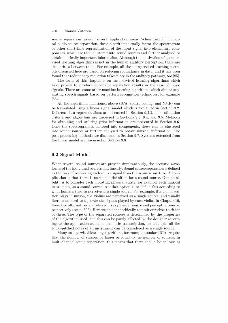
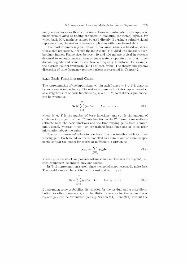
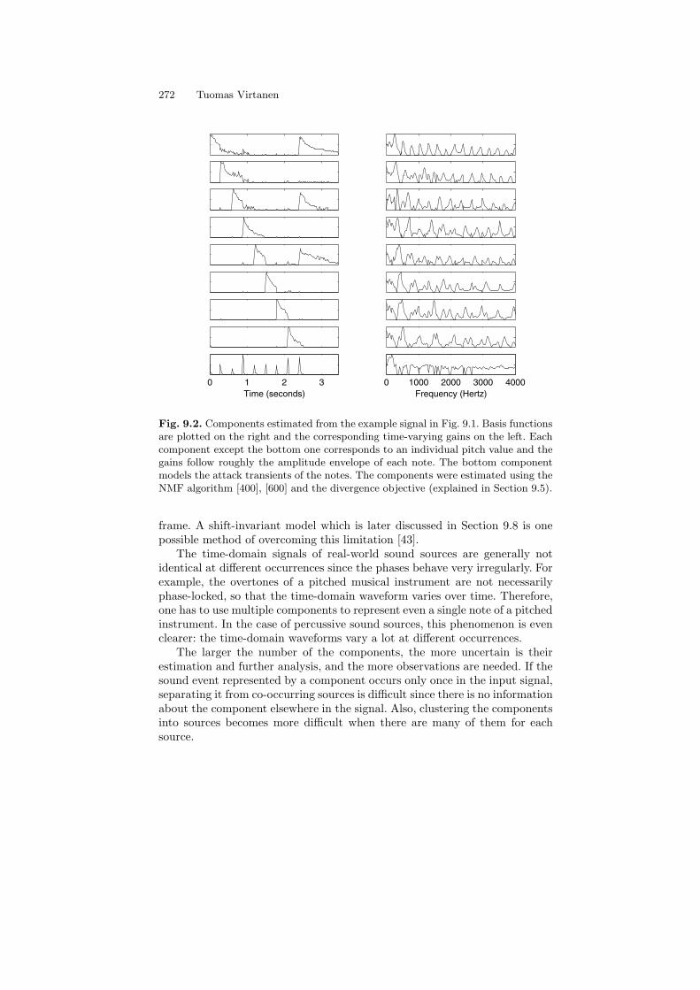
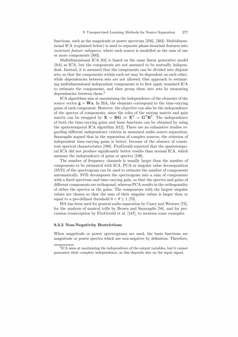
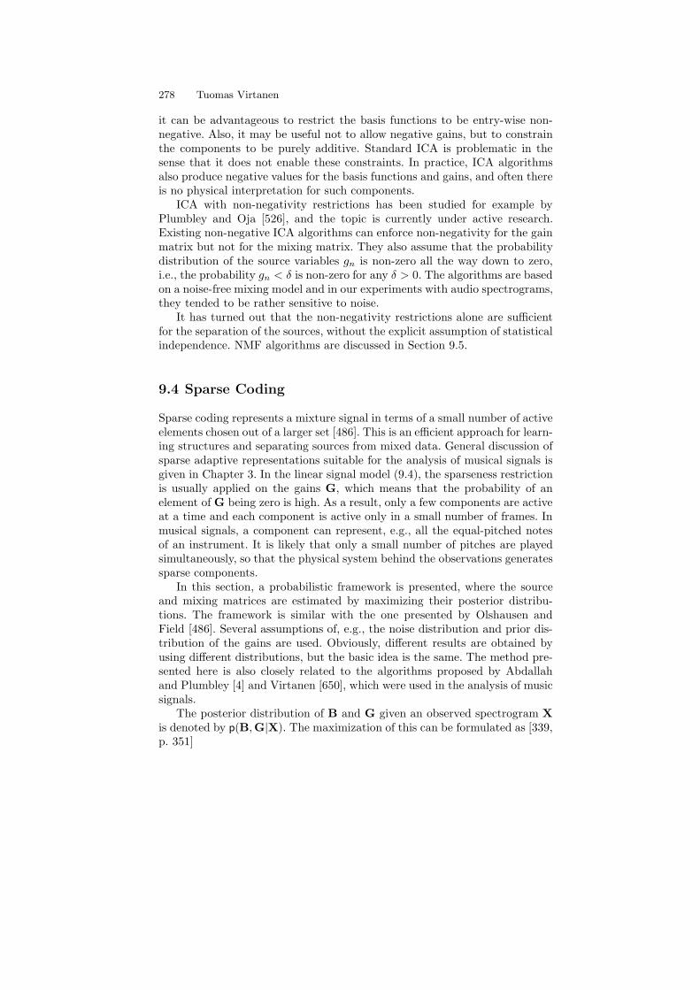
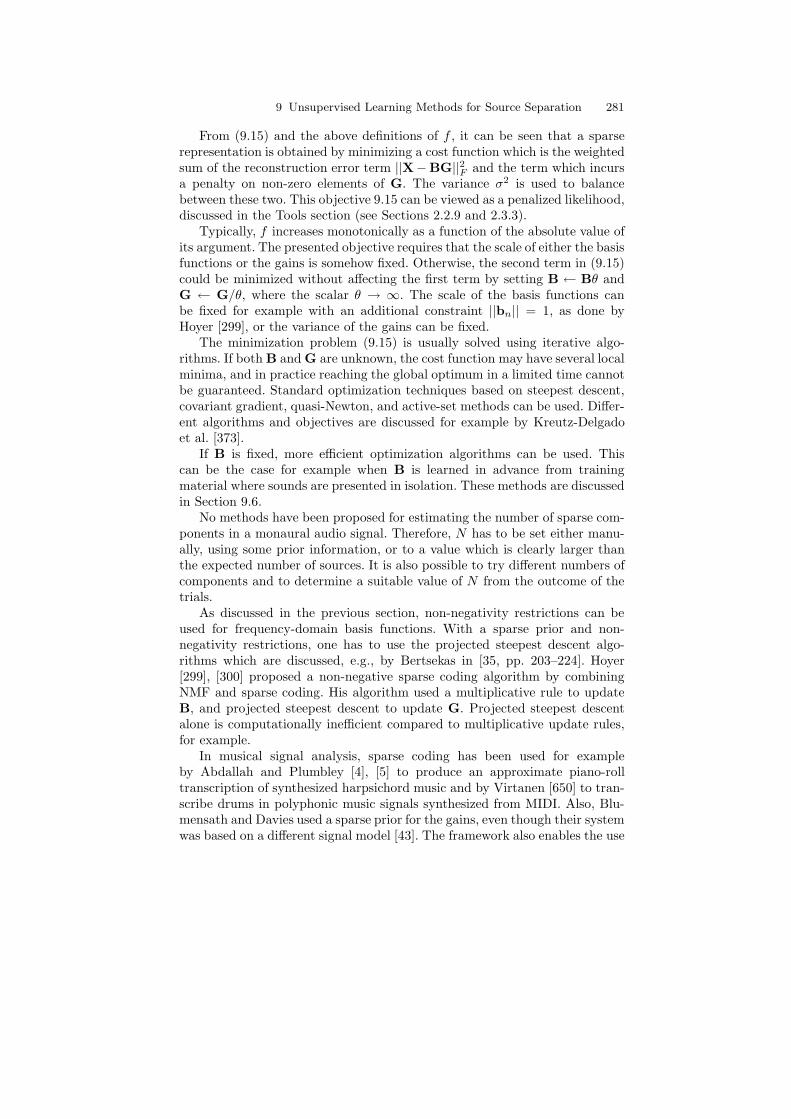
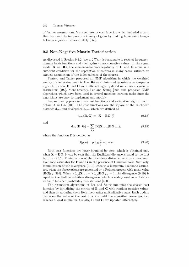
Figure 9.1 shows an example signal which consists of a diatonic scale anda C major chord played by an acoustic guitar. The signal was separated intocomponents using the NMF algorithm described in [600], and the resultingcomponents are depicted in Fig. 9.2. Each component corresponds roughly toone fundamental frequency: the basis functions are approximately harmonicand the time-varying gains follow the amplitude envelopes of the notes. Theseparation is not perfect because of estimation inaccuracies. For example, insome cases the gain of a decaying note drops to zero when a new note begins.

Factorization of the spectrogram into components with a fixed spectrumand a time-varying gain has been adopted as a part of the MPEG-7 patternrecognition framework [72], where the basis functions and the gains are usedas features for classification. Kim et al. [341] compared these to mel-frequencycepstral coefficients which are commonly used features in the classification ofaudio signals. In this study, mel-frequency cepstral coefficients performed bet-ter in the recognition of sound effects and speech than features based on ICAor NMF. However, final conclusions about the applicability of these methodsto sound source recognition have yet to be made. The spectral basis decompo-sition specified in MPEG-7 models the summation of components on a decibelscale, which makes it unlikely that the separated components correspond tophysical sound objects.

9.2.2 Data Representation

The model (9.1) presented in the previous section can be used with time-domain or frequency-domain observations and basis functions. Time-domain


Time (seconds)

Fre

qu

en

cy (

He

rtz)

0 0.5 1 1.5 2 2.5 3 3.50

500

1000

1500

2000

2500

3000

3500

4000

4500

5000

Fig. 9.1. Spectrogram of an example signal which consist of a diatonic scale fromC5 to C6, followed by a C major chord (simultaneous notes C5, E4, and G5), playedby an acoustic guitar. The notes are not damped, meaning that consecutive notesoverlap.

observation vector xt is the signal within frame t directly, whereas a frequency-domain observation vector is obtained by applying a chosen transformation tothis. The representation of the signal and the basis functions have to be thesame. ICA and sparse coding allow the use of any short-time signal represen-tation, whereas for NMF, only a frequency-domain representation is appro-priate. Naturally, the representation has a significant effect on performance.The advantages and disadvantages of different representations are consideredin this section. For a more extensive discussion, see Casey [70] or Smaragdis[598].

Time-Domain Representation

Time-domain representations are straightforward to compute, and all the in-formation is preserved when an input signal is segmented into frames and win-dowed. However, time-domain basis functions are problematic in the sense thata single basis function alone cannot represent a meaningful sound source: thephase of the signal within each frame varies depending on the frame position.In the case of a short-duration percussive source, for example, a separate basisfunction is needed for every possible position of the sound event within the

272 Tuomas Virtanen

0 1 2 3

Time (seconds)

0 1000 2000 3000 4000

Frequency (Hertz)

Fig. 9.2. Components estimated from the example signal in Fig. 9.1. Basis functionsare plotted on the right and the corresponding time-varying gains on the left. Eachcomponent except the bottom one corresponds to an individual pitch value and thegains follow roughly the amplitude envelope of each note. The bottom componentmodels the attack transients of the notes. The components were estimated using theNMF algorithm [400], [600] and the divergence objective (explained in Section 9.5).

frame. A shift-invariant model which is later discussed in Section 9.8 is onepossible method of overcoming this limitation [43].

The time-domain signals of real-world sound sources are generally notidentical at different occurrences since the phases behave very irregularly. Forexample, the overtones of a pitched musical instrument are not necessarilyphase-locked, so that the time-domain waveform varies over time. Therefore,one has to use multiple components to represent even a single note of a pitchedinstrument. In the case of percussive sound sources, this phenomenon is evenclearer: the time-domain waveforms vary a lot at different occurrences.

The larger the number of the components, the more uncertain is theirestimation and further analysis, and the more observations are needed. If thesound event represented by a component occurs only once in the input signal,separating it from co-occurring sources is difficult since there is no informationabout the component elsewhere in the signal. Also, clustering the componentsinto sources becomes more difficult when there are many of them for eachsource.


Separation algorithms which operate on time-domain signals have beenproposed for example by Dubnov [157], Jang and Lee [314], and Blumensathand Davies [43]. Abdallah and Plumbley [3], [2] found that the independentcomponents analysed from time-domain music and speech signals were similarto a wavelet or short-time DFT basis. They trained the basis functions usingseveral days of radio output from BBC Radio 3 and 4 stations.

Frequency-Domain Representation

When using a frequency transform such as the DFT, the phases of thecomplex-valued transform can be discarded by considering only the mag-nitude or power spectrum. Even though some information is lost, this alsoeliminates the phase-related problems of time-domain representations. Unliketime-domain basis functions, many real-world sounds can be rather well ap-proximated with a fixed magnitude spectrum and a time-varying gain, as seenin Figs. 9.1 and 9.2, for example. Sustained instruments in particular tend tohave a stationary spectrum after the attack transient.

In most systems aimed at the separation of sound sources, DFT and afixed window size is applied, but the estimation algorithms allow the useof any time-frequency representation. For example, a logarithmic spacing offrequency bins has been used [58], which is perceptually and musically moreplausible than a constant spectral resolution.

The linear summation of time-domain signals does not imply the linearsummation of their magnitude or power spectra, since phases of the sourcesignals affect the result. When two signals sum in the time domain, theircomplex-valued DFTs sum linearly, X(k) = Y1(k) + Y2(k), but this equalitydoes not apply for the magnitude or power spectra. However, provided thatthe phases of Y1(k) and Y2(k) are uniformly distributed and independent ofeach other, we can write

E{|X(k)|2} = |Y1(k)|2 + |Y2(k)|2, (9.5)

where E{·} denotes expectation. This means that in the expectation sense,we can approximate time-domain summation in the power spectral domain, aresult which holds for more than two sources as well. Even though magnitudespectrogram representation has been widely used and it often produces goodresults, it does not have similar theoretical justification. Since the summationis not exact, use of phaseless basis functions causes an additional source oferror. Also, a phase generation method has to be implemented if the sourcesare to be synthesized separately. These are discussed in Section 9.7.3.

The human auditory system has a large dynamic range: the differencebetween the threshold of hearing and the threshold of pain is approximately100 dB [550]. Unsupervised learning algorithms tend to be more sensitive tohigh-energy observations. If sources are estimated from the power spectrum,some methods fail to separate low-energy sources even though they would be

274 Tuomas Virtanen

perceptually and musically meaningful. This problem has been noticed, e.g.,by FitzGerald in the case of percussive source separation [186, pp. 93–100].To overcome the problem, he used an algorithm which processed separatelyhigh-frequency bands which contain low-energy sources, such as hi-hats andcymbals [187]. Vincent and Rodet [648] addressed the same problem. Theyproposed a model in which the noise was additive in the log-spectral domain.The numerical range of a logarithmic spectrum is compressed, which increasesthe sensitivity to low-energy sources. Additive noise in the log-spectral domaincorresponds to multiplicative noise in power spectral domain, which was alsoassumed in the system proposed by Abdallah and Plumbley [5]. Virtanenproposed the use of perceptually motivated weights [651]. He used a weightedcost function in which the observations were weighted so that the quantitativesignificance of the signal within each critical band was equal to its contributionto the total loudness.

9.3 Independent Component Analysis

ICA has been successfully used in several ‘blind’ source separation tasks, wherevery little or no prior information is available about the source signals. Oneof its original target applications was multi-channel sound source separation,but it has also had several other uses. ICA attempts to separate sources byidentifying latent signals that are maximally independent. In practice, thisusually leads to the separation of meaningful sound sources.

Mathematically, statistical independence is defined in terms of probabil-ity densities: random variables x and y are said to be independent if theirjoint probability distribution function1

p(x, y) is a product of the marginaldistribution functions, p(x, y) = p(x)p(y).

The dependence between two variables can be measured in several ways.Mutual information is a measure of the information that given random vari-ables have on some other random variables [304]. The dependence is alsoclosely related to the Gaussianity of the distribution of the variables. Accord-ing to the central limit theorem, the distribution of the sum of independentvariables is more Gaussian than their original distributions, under certain con-ditions. Therefore, some ICA algorithms aim at separating output variableswhose distributions are as far from Gaussian as possible.

The signal model in ICA is linear: K observed variables x1, . . . , xK aremodelled as linear combinations of N source variables g1, . . . , gN . In a vector-matrix form, this can be written as

x = Bg, (9.6)

where x =[

x1, . . . xK

]T

is an observation vector, [B]k,n = bk,n is a mixing

matrix, and g =[

g1, . . . , gN

]T

is a source vector. Both B and g are unknown.

1The concept of probability distribution function is described in Chapter 2.


The standard ICA requires that the number of observed variables K (thenumber of sensors) be equal to the number of sources N . In practice, the num-ber of sensors can also be larger than the number of sources, because the vari-ables are typically decorrelated using principal component analysis (PCA; seeChapter 2), and if the desired number of sources is less than the number ofvariables, only the principal components corresponding to the largest eigen-values are selected.

As another pre-processing step, the observed variables are usually centredby subtracting the mean and their variance is normalized to the unity. Thecentred and whitened data observation vector x is obtained from the originalobservation vector x by

x = V(x − µ), (9.7)

where µ is the empirical mean of the observation vector, and V is a whiteningmatrix, which is often obtained from the eigenvalue decomposition of theempirical covariance matrix of the observations [304]. The empirical meanand covariance matrix are explained in Chapter 2.

To simplify the notation, it is assumed that the data x in (9.6) is alreadycentred and decorrelated, so that K = N . The core ICA algorithm carriesout the estimation of an unmixing matrix W ≈ B−1, assuming that B isinvertible. Independent components are obtained by multiplying the whitenedobservations by the estimate of the unmixing matrix, to result in the sourcevector estimate g:

g = Wx. (9.8)

The matrix W is estimated so that the output variables, i.e., the elementsof g, become maximally independent. There are several criteria and algo-rithms for achieving this. The criteria, such as non-Gaussianity and mutualinformation, are usually measured using high-order cumulants such as kurto-sis, or expectations of other non-quadratic functions [304]. ICA can be alsoviewed as an extension of PCA. The basic PCA decorrelates variables so thatthey are independent up to second-order statistics. It can be shown that ifthe variables are uncorrelated after taking a suitable non-linear function, thehigher-order statistics of the original variables are independent, too. Thus,ICA can be viewed as a non-linear decorrelation method.

Compared with the previously presented linear model (9.3), the standardICA model (9.6) is exact, i.e., it does not contain the residual term. Somespecial techniques can be used in the case of the noisy signal model (9.3),but often noise is just considered as an additional source variable. Because ofthe dimension reduction with PCA, Bg gives an exact model for the PCA-transformed observations but not necessarily for the original ones.

There are several ICA algorithms, and some implementations are freelyavailable, such as FastICA [302], [182] and JADE [65]. Computationally quiteefficient separation algorithms can be implemented based on FastICA, forexample.

276 Tuomas Virtanen

9.3.1 Independent Subspace Analysis

The idea of independent subspace analysis (ISA) was originally proposed byHyvarinen and Hoyer [303]. It combines the multidimensional ICA with in-variant feature extraction, which are shortly explained later in this section.After the work of Casey and Westner [73], the term ISA has been commonlyused to denote techniques which apply ICA to factor the spectrogram of amonaural audio signal to separate sound sources. ISA provides a theoreticalframework for the whole separation procedure described in this chapter, in-cluding spectrogram representation, decomposition by ICA, and clustering.Some authors use the term ISA also to refer to methods where some otheralgorithm than ICA is used for the factorization [648].

The general ISA procedure consists of the following steps:

1. Calculate the magnitude spectrogram X (or some other representation)of the input signal.

2. Apply PCA2 on the matrix X of size (K × T ) to estimate the numberof components N and to obtain whitening and dewhitening matrices V

and V+, respectively. A centred, decorrelated, and dimensionally reducedobservation matrix X of size (N × T ) is obtained as X = V(X − µ1T),where 1 is a all-ones vector of length T .

3. Apply ICA to estimate an unmixing matrix W. B and G are obtained asB = W−1 and G = WX.

4. Invert the decorrelation operation in Step 2 in order to get the mixingmatrix B = V+B and source matrix G = G + WVµ1T for the originalobservations X.

5. Cluster the projected components to sources (see Section 9.7.1).

The above steps are explained in more detail below. Depending on the appli-cation, not all of them may be necessary. For example, prior information canbe used to set the number of components in Step 2.

The basic ICA is not directly suitable for the separation of one-channelsignals, since the number of sensors has to be larger than or equal to thenumber of sources. Short-time signal processing can be used in an attemptto overcome this limitation. Taking a frequency transform such as DFT, eachfrequency bin can be considered as a sensor which produces an observation ineach frame. With the standard linear ICA model (9.6), the signal is modelledas a sum of components, each of which has a static spectrum (or some otherbasis function) and a time-varying gain.

The spectrogram factorization has its motivation in invariant feature ex-traction, which is a technique proposed by Kohonen [356]. The short-timespectrum can be viewed as a set of features calculated from the input signal.As discussed in Section 9.2.2, it is often desirable to have shift-invariant basis

2Singular value decomposition can also be used to estimate the number of com-ponents [73].


functions, such as the magnitude or power spectrum [356], [303]. Multidimen-sional ICA (explained below) is used to separate phase-invariant features intoinvariant feature subspaces, where each source is modelled as the sum of oneor more components [303].

Multidimensional ICA [64] is based on the same linear generative model(9.6) as ICA, but the components are not assumed to be mutually indepen-dent. Instead, it is assumed that the components can be divided into disjointsets, so that the components within each set may be dependent on each other,while dependencies between sets are not allowed. One approach to estimat-ing multidimensional independent components is to first apply standard ICAto estimate the components, and then group them into sets by measuringdependencies between them.3

ICA algorithms aim at maximizing the independence of the elements of thesource vector g = Wx. In ISA, the elements correspond to the time-varyinggains of each component. However, the objective can also be the independenceof the spectra of components, since the roles of the mixing matrix and gainmatrix can be swapped by X = BG ⇔ XT = GTBT. The independenceof both the time-varying gains and basis functions can be obtained by usingthe spatiotemporal ICA algorithm [612]. There are no exhaustive studies re-garding different independence criteria in monaural audio source separation.Smaragdis argued that in the separation of complex sources, the criterion ofindependent time-varying gains is better, because of the absence of consis-tent spectral characteristics [598]. FitzGerald reported that the spatiotempo-ral ICA did not produce significantly better results than normal ICA, whichassumes the independence of gains or spectra [186].

The number of frequency channels is usually larger than the number ofcomponents to be estimated with ICA. PCA or singular value decomposition(SVD) of the spectrogram can be used to estimate the number of componentsautomatically. SVD decomposes the spectrogram into a sum of componentswith a fixed spectrum and time-varying gain, so that the spectra and gains ofdifferent components are orthogonal, whereas PCA results in the orthogonalityof either the spectra or the gains. The components with the largest singularvalues are chosen so that the sum of their singular values is larger than orequal to a pre-defined threshold 0 < θ ≤ 1 [73].

ISA has been used for general audio separation by Casey and Westner [73],for the analysis of musical trills by Brown and Smaragdis [58], and for per-cussion transcription by FitzGerald et al. [187], to mention some examples.

9.3.2 Non-Negativity Restrictions

When magnitude or power spectrograms are used, the basis functions aremagnitude or power spectra which are non-negative by definition. Therefore,

3ICA aims at maximizing the independence of the output variables, but it cannotguarantee their complete independence, as this depends also on the input signal.

278 Tuomas Virtanen

it can be advantageous to restrict the basis functions to be entry-wise non-negative. Also, it may be useful not to allow negative gains, but to constrainthe components to be purely additive. Standard ICA is problematic in thesense that it does not enable these constraints. In practice, ICA algorithmsalso produce negative values for the basis functions and gains, and often thereis no physical interpretation for such components.

ICA with non-negativity restrictions has been studied for example byPlumbley and Oja [526], and the topic is currently under active research.Existing non-negative ICA algorithms can enforce non-negativity for the gainmatrix but not for the mixing matrix. They also assume that the probabilitydistribution of the source variables gn is non-zero all the way down to zero,i.e., the probability gn < δ is non-zero for any δ > 0. The algorithms are basedon a noise-free mixing model and in our experiments with audio spectrograms,they tended to be rather sensitive to noise.

It has turned out that the non-negativity restrictions alone are sufficientfor the separation of the sources, without the explicit assumption of statisticalindependence. NMF algorithms are discussed in Section 9.5.

9.4 Sparse Coding

Sparse coding represents a mixture signal in terms of a small number of activeelements chosen out of a larger set [486]. This is an efficient approach for learn-ing structures and separating sources from mixed data. General discussion ofsparse adaptive representations suitable for the analysis of musical signals isgiven in Chapter 3. In the linear signal model (9.4), the sparseness restrictionis usually applied on the gains G, which means that the probability of anelement of G being zero is high. As a result, only a few components are activeat a time and each component is active only in a small number of frames. Inmusical signals, a component can represent, e.g., all the equal-pitched notesof an instrument. It is likely that only a small number of pitches are playedsimultaneously, so that the physical system behind the observations generatessparse components.

In this section, a probabilistic framework is presented, where the sourceand mixing matrices are estimated by maximizing their posterior distribu-tions. The framework is similar with the one presented by Olshausen andField [486]. Several assumptions of, e.g., the noise distribution and prior dis-tribution of the gains are used. Obviously, different results are obtained byusing different distributions, but the basic idea is the same. The method pre-sented here is also closely related to the algorithms proposed by Abdallahand Plumbley [4] and Virtanen [650], which were used in the analysis of musicsignals.

The posterior distribution of B and G given an observed spectrogram X

is denoted by p(B,G|X). The maximization of this can be formulated as [339,p. 351]


maxB,G

p(B,G|X) ∝ maxB,G

p(X|B,G)p(B,G), (9.9)

where p(X|B,G) is the probability of observing X given B and G, andp(B,G) is the joint prior distribution of B and G. The concepts of proba-bility distribution function, conditional probability distribution function, andmaximum a posteriori estimation are described in Chapter 2.

For mathematical tractability, it is typically assumed that the noise (theresidual term in (9.3)) is i.i.d.; independent from the model BG, and normallydistributed with variance σ2 and zero mean. The likelihood of B and G (seeSection 2.2.5 for the eplanation of likelihood functions) can be written as

p(X|B,G) =∏

t,k

1

σ√

2πexp

(

− ([X]k,t − [BG]k,t)2

2σ2

)

. (9.10)

It is further assumed here that B has a uniform prior, so that p(B,G) ∝p(G). Each time-varying gain [G]n,t is assumed to have a sparse probabilitydistribution function of the exponential form

p([G]n,t) =1

Zexp (−f([G]n,t)) . (9.11)

A normalization factor Z has to be used so that the density function sums tounity. The function f is used to control the shape of the distribution and ischosen so that the distribution is uni-modal and peaked at zero with heavytails. Some examples are given later.

For simplicity, all the entries of G are assumed to be independent fromeach other, so that the probability distribution function of G can be writtenas a product of the marginal densities:

p(G) =∏

n,t

1

Zexp (−f([G]n,t)) . (9.12)

It is obvious that in practice the gains are not independent of each other,but this approximation is done to simplify the calculations. From the abovedefinitions we get

maxB,G

p(B,G|X) ∝ maxB,G

∏

t,k

1

σ√

2πexp

(

− ([X]k,t − [BG]k,t)2

2σ2

)

×∏

n,t

1

Zexp (−f([G]n,t)) .

(9.13)

By taking a logarithm, the products become summations, and the exp-operators and scaling terms can be discarded. This can be done since logarithmis order preserving and therefore does not affect the maximization. The signis changed to obtain a minimization problem

280 Tuomas Virtanen

minB,G

∑

t,k

([X]k,t − [BG]k,t)2

2σ2+∑

n,t

f([G]n,t), (9.14)

which can be written as

minB,G

1

2σ2||X− BG||2F +

∑

n,t

f([G]n,t), (9.15)

where the Frobenius norm of a matrix is defined as

||Y||F =

√

∑

i,j

[Y]2i,j . (9.16)

In (9.15), the function f is used to penalize ‘active’ (non-zero) entries ofG. For example, Olshausen and Field [486] suggested the functions f(x) =log(1 + x2), f(x) = |x|, and f(x) = x2. In audio source separation, Benaroyaet al. [32] and Virtanen [650] have used f(x) = |x|. The prior distributionused by Abdallah and Plumbley [2], [4] corresponds to the function

f(x) =

{

|x|, |x| ≥ µ,

µ(1 − α) + α|x|, |x| < µ,(9.17)

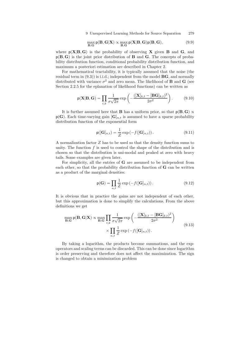
where the parameters µ and α control the relative mass of the central peak inthe prior, and the term µ(1−α) is used to make the function continuous at x =±µ. All these functions give a smaller cost and a higher prior probability forgains near zero. The cost function f(x) = |x| and the corresponding Laplacianprior p(x) = 1

2exp(−|x|) are illustrated in Fig. 9.3. Systematic large-scale

evaluations of different sparse priors in audio signals have not been carriedout. Naturally, the distributions depend on source signals, and also on thedata representation.

−2 0 20

0.2

0.4

[G]n,t

p([

G] n

,t)

−2 0 20

1

2

3

[G]n,t

f ([

G] n

,t)

Fig. 9.3. The cost function f(x) = |x| (left) and the corresponding Laplacian priordistribution p(x) = 1

2exp(−|x|) (right). Values of G near zero are given a smaller

cost and a higher probability.


From (9.15) and the above definitions of f , it can be seen that a sparserepresentation is obtained by minimizing a cost function which is the weightedsum of the reconstruction error term ||X−BG||2F and the term which incursa penalty on non-zero elements of G. The variance σ2 is used to balancebetween these two. This objective 9.15 can be viewed as a penalized likelihood,discussed in the Tools section (see Sections 2.2.9 and 2.3.3).

Typically, f increases monotonically as a function of the absolute value ofits argument. The presented objective requires that the scale of either the basisfunctions or the gains is somehow fixed. Otherwise, the second term in (9.15)could be minimized without affecting the first term by setting B ← Bθ andG ← G/θ, where the scalar θ → ∞. The scale of the basis functions canbe fixed for example with an additional constraint ||bn|| = 1, as done byHoyer [299], or the variance of the gains can be fixed.

The minimization problem (9.15) is usually solved using iterative algo-rithms. If both B and G are unknown, the cost function may have several localminima, and in practice reaching the global optimum in a limited time cannotbe guaranteed. Standard optimization techniques based on steepest descent,covariant gradient, quasi-Newton, and active-set methods can be used. Differ-ent algorithms and objectives are discussed for example by Kreutz-Delgadoet al. [373].

If B is fixed, more efficient optimization algorithms can be used. Thiscan be the case for example when B is learned in advance from trainingmaterial where sounds are presented in isolation. These methods are discussedin Section 9.6.

No methods have been proposed for estimating the number of sparse com-ponents in a monaural audio signal. Therefore, N has to be set either manu-ally, using some prior information, or to a value which is clearly larger thanthe expected number of sources. It is also possible to try different numbers ofcomponents and to determine a suitable value of N from the outcome of thetrials.

As discussed in the previous section, non-negativity restrictions can beused for frequency-domain basis functions. With a sparse prior and non-negativity restrictions, one has to use the projected steepest descent algo-rithms which are discussed, e.g., by Bertsekas in [35, pp. 203–224]. Hoyer[299], [300] proposed a non-negative sparse coding algorithm by combiningNMF and sparse coding. His algorithm used a multiplicative rule to updateB, and projected steepest descent to update G. Projected steepest descentalone is computationally inefficient compared to multiplicative update rules,for example.

In musical signal analysis, sparse coding has been used for exampleby Abdallah and Plumbley [4], [5] to produce an approximate piano-rolltranscription of synthesized harpsichord music and by Virtanen [650] to tran-scribe drums in polyphonic music signals synthesized from MIDI. Also, Blu-mensath and Davies used a sparse prior for the gains, even though their systemwas based on a different signal model [43]. The framework also enables the use

282 Tuomas Virtanen

of further assumptions. Virtanen used a cost function which included a termthat favoured the temporal continuity of gains by making large gain changesbetween adjacent frames unlikely [650].

9.5 Non-Negative Matrix Factorization

As discussed in Section 9.3.2 (see p. 277), it is reasonable to restrict frequency-domain basis functions and their gains to non-negative values. In the signalmodel X ≈ BG, the element-wise non-negativity of B and G alone is asufficient condition for the separation of sources in many cases, without anexplicit assumption of the independence of the sources.

Paatero and Tatter proposed an NMF algorithm in which the weightedenergy of the residual matrix X−BG was minimized by using a least-squaresalgorithm where B and G were alternatingly updated under non-negativityrestrictions [492]. More recently, Lee and Seung [399, 400] proposed NMFalgorithms which have been used in several machine learning tasks since thealgorithms are easy to implement and modify.

Lee and Seung proposed two cost functions and estimation algorithms toobtain X ≈ BG [400]. The cost functions are the square of the Euclideandistance deuc and divergence ddiv, which are defined as

deuc(B,G) = ||X − BG||2F (9.18)

andddiv(B,G) =

∑

k,t

D([X]k,t, [BG]k,t), (9.19)

where the function D is defined as

D(p, q) = p logp

q− p + q. (9.20)

Both cost functions are lower-bounded by zero, which is obtained onlywhen X = BG. It can be seen that the Euclidean distance is equal to the firstterm in (9.15). Minimization of the Euclidean distance leads to a maximumlikelihood estimator for B and G in the presence of Gaussian noise. Similarly,minimization of the divergence (9.19) leads to a maximum likelihood estima-tor, when the observations are generated by a Poisson process with mean value[BG]k,t [399]. When

∑

k,t[X]k,t =∑

k,t[BG]k,t = 1, the divergence (9.19) isequal to the Kullback–Leibler divergence, which is widely used as a distancemeasure between probability distributions [400].

The estimation algorithms of Lee and Seung minimize the chosen costfunction by initializing the entries of B and G with random positive values,and then by updating them iteratively using multiplicative rules. Each updatedecreases the value of the cost function until the algorithm converges, i.e.,reaches a local minimum. Usually, B and G are updated alternately.


The update rules for the Euclidean distance are given as

B ← B.×(XGT)./(BGGT) (9.21)

andG ← G.×(BTX)./(BTBG), (9.22)

where .× and ./ denote the element-wise multiplication and division, respec-tively. The update rules for the divergence are given as

B ← B.×(X./BG)GT

1GT(9.23)

and

G ← G.×BT(X./BG)

BT1, (9.24)

where 1 is an all-ones K-by-T matrix, and X

Ydenotes the element-wise division

of matrices X and Y.To summarize, the algorithm for NMF is as follows:

Algorithm 9.1: Non-Negative Matrix Factorization

1. Initialize each entry of B and G with the absolute values of Gaussian noise.2. Update G using either (9.22) or (9.24) depending on the chosen cost function.3. Update B using either (9.21) or (9.23) depending on the chosen cost function.4. Repeat Steps (2)–(3) until the values converge.

Methods for the estimation of the number of components have not beenproposed, but all the methods suggested in Section 9.4 are applicable in NMF,too. The multiplicative update rules have proven to be more efficient than forexample the projected steepest-descent algorithms [400], [299], [5].

NMF can be used only for a non-negative observation matrix and thereforeit is not suitable for the separation of time-domain signals. However, whenused with the magnitude or power spectrogram, the basic NMF can be usedto separate components without prior information other than the element-wise non-negativity. In particular, factorization of the magnitude spectrogramusing the divergence often produces relatively good results. The divergencecost of an individual observation [X]k,t is linear as a function of the scale ofthe input, since D(αp, αq) = αD(p, q) for any positive scalar α, whereas forthe Euclidean cost the dependence is quadratic. Therefore, the divergence ismore sensitive to small-energy observations.

NMF does not explicitly aim at components which are statistically in-dependent from each other. However, it has been proved that under certainconditions, the non-negativity restrictions are theoretically sufficient for sep-arating statistically independent sources [525]. It has not been investigatedwhether musical signals fulfill these conditions, and whether NMF implement

284 Tuomas Virtanen

a suitable estimation algorithm. Currently, there is no comprehensive theo-retical explanation of why NMF works so well in sound source separation.If a mixture spectrogram is a sum of sources which have a static spectrumwith a time-varying gain, and each of them is active in at least one frameand frequency line in which the other components are inactive, the objec-tive function of NMF is minimized by a decomposition in which the sourcesare separated perfectly. However, real-world music signals rarely fulfill theseconditions. When two or more more sources are present simultaneously at alltimes, the algorithm is likely to represent them with a single component.

In the analysis of music signals, the basic NMF has been used by Smaragdisand Brown [600], and extended versions of the algorithm have been pro-posed for example by Virtanen [650] and Smaragdis [599]. The problem ofthe large dynamic range of musical signals has been addressed e.g. by Abdal-lah and Plumbley [5]. By assuming multiplicative gamma-distributed noise inthe power spectral domain, they derived the cost function

D(p, q) =p

q− 1 + log

q

p, (9.25)

to be used instead of (9.20). Compared to the Euclidean distance (9.18) anddivergence (9.20), this distance measure is more sensitive to low-energy ob-servations. In our simulations, however, it did not produce results as good asthe Euclidean distance or the divergence did.

9.6 Prior Information about Sources

Manual transcription of music requires a lot of prior knowledge and training.The described separation algorithms used some general assumptions aboutthe sources in the core algorithms, such as independence or non-negativity,but also other prior information on the sources is often available. For examplein the analysis of pitched musical instruments, it is known in advance thatthe spectra of instruments are approximately harmonic. Unfortunately, it isdifficult to implement harmonicity restrictions in the models discussed earlier.

Prior knowledge can also be source-specific. The most common approach toincorporate prior information about sources in the analysis is to train source-specific basis functions in advance. Several approaches have been proposed.The estimation is usually done in two stages, which are

1. Learn source-specific basis functions from training material, such as mono-timbral and monophonic music. Also the characteristics of time-varyinggains can be stored, for example by modelling their distribution.

2. Represent a polyphonic signal as a weighted sum of the basis functions ofall the instruments. Estimate the gains and keep the basis functions fixed.

It is not yet known whether automatic music transcription is possible withoutany source-specific prior knowledge, but obviously this has the potential tomake the task much easier.


Several methods have been proposed for training the basis functions inadvance. The most straightforward choice is to also separate the trainingsignal using some of the described methods. For example, Jang and Lee [314]used ISA to train basis functions for two sources separately. Benaroya et al.[32] suggested the use of non-negative sparse coding, but they also tested usingthe spectra of random frames of the training signal as the basis functions orgrouping similar frames to obtain the basis functions. They reported thatnon-negative sparse coding and the grouping algorithm produced the bestresults [32]. Gautama and Van Halle compared three different self-organizingmethods in the training of basis functions [204].

The training can be done in a more supervised manner by using a sepa-rate set of training samples for each basis function. For example in the drumtranscription systems proposed by FitzGerald et al. [188] and Paulus andVirtanen [505], the basis function for each drum instrument was calculatedfrom isolated samples of each drum. It is also possible to generate the basisfunctions manually, for example so that each of them corresponds to a singlepitch. Lepain used frequency-domain harmonic combs as the basis functions,and parameterized the rough shape of the spectrum using a slope parameter[403]. Sha and Saul trained the basis function for each discrete fundamentalfrequency using a speech database with annotated pitch [579].

In practice, it is difficult to train basis functions for all the possible sourcesbeforehand. An alternative is to use trained or generated basis functions whichare then adapted to the observed data. For example, Abdallah and Plumbleyinitialized their non-negative sparse coding algorithm with basis functions thatconsisted of harmonic spectra with a quarter-tone pitch spacing [5]. After theinitialization, the algorithm was allowed to adapt these.

Once the basis functions have been trained, the observed input signal isrepresented using them. Sparse coding and non-negative matrix factorizationtechniques are feasible also in this task. Usually the reconstruction error be-tween the input signal and the model is minimized while using a small numberof active basis functions (sparseness constraint). For example, Benaroya et al.proposed an algorithm which minimizes the energy of the reconstruction errorwhile restricting the gains to be non-negative and sparse [32].

If the sparseness criterion is not used, a matrix G reaching the globalminimum of the reconstruction error can be usually found rather easily. If thegains are allowed to have negative values and the estimation criterion is theenergy of the residual, the standard least-squares solution

G = (BTB)−1BTX (9.26)

produces the optimal gains (assuming that the previously trained basis func-tions are linearly independent) [339, pp. 220–226]. If the gains are restrictedto non-negative values, the least-squares solution is obtained using the non-negative least-squares algorithm [397, p. 161]. When the basis functions,observations, and gains are restricted to non-negative values, the global min-imum of the divergence (9.19) between the observations and the model can

286 Tuomas Virtanen

be computed by applying the multiplicative update (9.24) iteratively [563],[505]. Lepain minimized the sum of the absolute value of the error betweenthe observations and the model by using linear programming and the Simplexalgorithm [403].

The estimation of the gains can also be done in a framework which in-creases the probability of basis functions being non-zero in consecutive frames.For example, Vincent and Rodet used hidden Markov models (HMMs) tomodel the durations of the notes [648].

It is also possible to train prior distributions for the gains. Jang and Leeused standard ICA techniques to train time-domain basis functions for eachsource separately, and modelled the probability distribution function of thecomponent gains with a generalized Gaussian distribution which is a familyof density functions of the form p(x) ∝ exp(−|x|q) [314]. For an observedmixture signal, the gains were estimated by maximizing their posterior prob-ability.

9.7 Further Processing of the Components

The main motivation for separating an input signal into components is thateach component usually represents a musically meaningful entity, such as apercussive instrument or all the equal-pitched notes of an instrument. Separa-tion alone does not solve the transcription problem, but has the potential tomake it much easier. For example, estimation of the fundamental frequencyof an isolated sound is easier than multiple fundamental frequency estimationin a mixture signal.

9.7.1 Associating Components with Sources

If the basis functions are estimated from a mixture signal, we do not knowwhich component is produced by which source. Since each source is modelledas a sum of one or more components, we need to associate the componentsto sources. There are roughly two ways to do this. In the unsupervised classi-fication framework, component clusters are formed based on some similaritymeasure, and these are interpreted as sources. Alternately, if prior informa-tion about the sources is available, the components can be classified to sourcesbased on their distance to source models. Naturally, if pre-trained basis func-tions are used for each source, the source of each basis function is known andclassification is not needed.

Pairwise dependence between the components can be used as a similaritymeasure for clustering. Even in the case of ICA, which aims at maximizing theindependence of the components, some dependencies may remain because itis possible that the input signal contains fewer independent components thanare to be separated.


Casey and Westner used the symmetric Kullback–Leibler divergence be-tween the probability distribution functions of basis functions as a distancemeasure, resulting in an independent component cross-entropy matrix (an ‘ix-egram’) [73]. Dubnov proposed a distance measure derived from the higher-order statistics of the basis functions or the gains [157]. Casey and Westner[73] and Dubnov [157] also suggested clustering algorithms for grouping thecomponents into sources. These try to minimize the inter-cluster dependenceand maximize the intra-cluster dependence.

For predefined sound sources, the association can be done using patternrecognition methods. Uhle et al. extracted acoustic features from each com-ponent to classify them either to a drum track or to a harmonic track [634].The features in their system included, for example, the percussiveness of thetime-varying gain, and the noise-likeness and dissonance of the spectrum. An-other system for separating drums from polyphonic music was proposed byHelen and Virtanen. They trained a support vector machine (SVM) using thecomponents extracted from a set of drum tracks and polyphonic music sig-nals without drums. Different acoustic features were evaluated, including theabove-mentioned ones, mel-frequency cepstral coefficients, and others [282].

9.7.2 Extraction of Musical Information

The separated components are usually analysed to obtain musically importantinformation, such as the onset and offset times and fundamental frequency ofeach component (assuming that they represent individual notes of a pitchedinstrument). Naturally, the analysis can be done by synthesizing the com-ponents and by using analysis techniques discussed elsewhere in this book.However, the synthesis stage is usually not needed, but analysis using the ba-sis functions and gains directly is likely to be more reliable, since the synthesisstage may cause some artifacts.

The onset and offset times of each component n are measured from thetime-varying gains gn,t, t = 1 . . . T . Ideally, a component is active when itsgain is non-zero. In practice, however, the gain may contain interference fromother sources and the activity detection has to be done with a more robustmethod.

Paulus and Virtanen [505] proposed an onset detection procedure that wasderived from the psychoacoustically motivated method of Klapuri [347]. Thegains of a component were compressed, differentiated, and lowpass filtered.In the resulting ‘accent curve’, all local maxima above a fixed threshold wereconsidered as sound onsets. For percussive sources or other instruments witha strong attack transient, the detection can be done simply by locating localmaxima in the gain functions, as done by FitzGerald et al. [188].

The detection of sound offsets is a more difficult problem, since the am-plitude envelope of a note can be exponentially decaying. Methods to be usedin the presented framework have not been proposed.

288 Tuomas Virtanen

There are several different possibilities for the estimation of the funda-mental frequency of a pitched component. For example, prominent peaks canbe located from the spectrum and the two-way mismatch procedure of Maherand Beauchamp [428] can be used, or the fundamental period can be esti-mated from the autocorrelation function which is obtained by inverse Fouriertransforming the power spectrum. In our experiments, the enhanced auto-correlation function proposed by Tolonen and Karjalainen [627] was found toproduce good results (see p. 253 in this volume). In practice, a component mayrepresent more than one pitch. This happens especially when the pitches arealways present simultaneously, as is the case in a chord, for example. No meth-ods have been proposed to detect this situation. Whether or not a componentis pitched can be estimated, e.g., from features based on the component [634],[282].

Some systems use fixed basis functions which correspond to certain funda-mental frequency values [403], [579]. In this case, the fundamental frequencyof each basis function is of course known.

9.7.3 Synthesis

Synthesis of the separated components is needed at least when one wants tolisten to them, which is a convenient way to roughly evaluate the quality of theseparation. Synthesis from time-domain basis functions is straightforward: thesignal of component n in frame t is generated by multiplying the basis functionbn by the corresponding gain gn,t, and adjacent frames are combined usingthe overlap-add method where frames are multiplied by a suitable windowfunction, delayed, and summed.

Synthesis from frequency-domain basis functions is not as trivial. The syn-thesis procedure includes calculation of the magnitude spectrum of a compo-nent in each frame, estimation of the phases to obtain the complex spectrum,and an inverse discrete Fourier transform (IDFT) to obtain the time-domainsignal. Adjacent frames are then combined using overlap-add. When magni-tude spectra are used as the basis functions, framewise spectra are obtainedas the product of the basis function with its gain. If power spectra are used, asquare root has to be taken, and if the frequency resolution is not linear,additional processing has to be done to enable synthesis using the IDFT.

A few alternative methods have been proposed for the phase generation.Using the phases of the original mixture spectrogram produces good syn-thesis quality when the components do not overlap significantly in time andfrequency [651]. However, applying the original phases and the IDFT may pro-duce signals which have unrealistic large values at frame boundaries, resultingin perceptually unpleasant discontinuities when the frames are combined us-ing overlap-add. The phase generation method proposed by Griffin and Lim[259] has also been used in synthesis (see for example Casey [70]). The methodfinds phases so that the error between the separated magnitude spectrogramand the magnitude spectrogram of the resynthesized time-domain signal is


minimized in the least-squares sense. The method can produce good synthesisquality especially for slowly varying sources with deterministic phase behav-iour. The least-squares criterion, however, gives less importance to low-energypartials and often leads to a degraded high-frequency content. The phase gen-eration problem has been recently addressed by Achan et al., who proposeda phase generation method based on a pre-trained autoregressive model [9].

9.8 Time-Varying Components

As mentioned above, the linear model (9.1) is efficient in the analysis of musicsignals since many musically meaningful entities can be rather well approxi-mated with a fixed spectrum and a time-varying gain. However, representationof sources with strongly time-varying spectrum requires several components,and each fundamental frequency value produced by a pitched instrument hasto be represented with a different component. Instead of using multiple com-ponents per source, more complex models can be constructed which alloweither a time-varying spectrum or a time-varying fundamental frequency foreach component. These are discussed in the following two subsections.

9.8.1 Time-Varying Spectra

Time-varying spectra of components can be obtained by replacing each basisfunction bn by a sequence of basis functions bn,τ , where τ = 0 . . . L− 1 is theframe index. If a frequency-domain representation is used, this means that astatic short-time spectrum of a component is replaced by a spectrogram oflength L frames.

The signal model for one component can be formulated as a convolutionbetween its spectrogram and time-varying gain. The model for a mixturespectrum of N components is given by

xt ≈N∑

n=1

L−1∑

τ=0

bn,τgn,t−τ . (9.27)

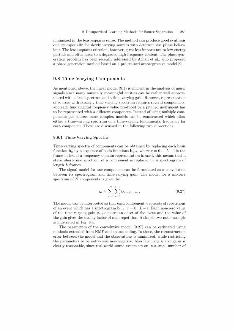
The model can be interpreted so that each component n consists of repetitionsof an event which has a spectrogram bn,τ , τ = 0...L− 1. Each non-zero valueof the time-varying gain gn,t denotes an onset of the event and the value ofthe gain gives the scaling factor of each repetition. A simple two-note exampleis illustrated in Fig. 9.4.

The parameters of the convolutive model (9.27) can be estimated usingmethods extended from NMF and sparse coding. In these, the reconstructionerror between the model and the observations is minimized, while restrictingthe parameters to be entry-wise non-negative. Also favouring sparse gains isclearly reasonable, since real-world sound events set on in a small number of

290 Tuomas Virtanen

Time (seconds)

Fre

quency (

Hert

z)

0 0.5 1 1.5 2 2.5 30

1000

2000

3000

4000

5000

Fig. 9.4. An example of the convolutive model (9.27) which allows time-varyingcomponents. The mixture spectrogram (upper left panel) contains the notes C#6and F#6 of the acoustic guitar, first played separately and then together. The upperright panels illustrate the learned note spectrograms and the lower panel shows theirtime-varying gains. In the gains, an impulse corresponds to the onset of a note. Thecomponents were estimated using a modified version of the algorithm proposed bySmaragdis in [599]. In the case of more complex signals, it is difficult to obtain suchclear impulses.

frames only. Virtanen [651] proposed an algorithm which is based on non-negative sparse coding, whereas that of Smaragdis [599] aims at minimizingthe divergence between the observation and the model while constraining non-negativity.

Arbitrarily long durations L may not be used if the basis functions areestimated from a mixture signal. When NL ≥ T , the input spectrogram canbe represented perfectly as a sum of concatenated event spectrograms (withoutseparation). Meaningful sources are likely to be separated only when NL ≪ T .In other words, estimation of several components with large L requires longinput signals.

In addition, the method proposed by Blumensath and Davies [43] can beformulated using (9.27). Their objective was to find sparse and shift-invariantdecompositions of a signal in the time domain. Their model allows an eventto begin at any time with one sample accuracy which makes the numberof free parameters in the model large. To reduce the dimensionality of theproblem, Blumensath and Davies proposed an algorithm which carried out


the optimization in a subspace of the parameters. They also included a sparseprior for the gains.

9.8.2 Time-Varying Fundamental Frequencies

In some cases, it is desirable to use a model which can represent differentpitch values of an instrument with a single component. For example, in thecase where a note with a certain pitch is present only during a short time,separating it from co-occurring sources is difficult. However, if other notes ofthe source with adjacent pitch values can be utilized, the estimation becomesmore reliable.

Varying fundamental frequencies are difficult to model using time-domainbasis functions or frequency-domain basis functions with linear frequency reso-lution. This is because changing the fundamental frequency of a basis functionis a non-linear operation which is difficult to implement in practice: if the fun-damental frequency is multiplied by a factor γ, the frequencies of the harmoniccomponents are also multiplied by γ; this can be viewed as a stretching of thespectrum. For an arbitrary value of γ, the stretching is difficult to perform ona discrete linear frequency resolution, at least using a simple operator whichcould be used in the unsupervised learning framework. The same holds as wellfor time-domain basis functions.

A logarithmic spacing of frequency bins makes it easier to represent varyingfundamental frequencies. A logarithmic scale consists of discrete frequenciesfrefβ

k−1, where k = 1 . . .K is the discrete frequency index, β > 1 is the ratiobetween adjacent frequency bins, and fref is a reference frequency in Hertzwhich can be selected arbitrarily. For example, β = 12

√2 produces a frequency

scale where the spacing between the frequencies is one semitone.On the logarithmic scale, the spacing of the partials of a harmonic sound

is independent of its fundamental frequency. For fundamental frequency f0,the overtone frequencies of a perfectly harmonic sound are mf0, where m > 0is an integer. On the logarithmic scale, the corresponding frequency indicesare k = logβ(m) + logβ(f0/fref), and thus the fundamental frequency affectsonly the offset logβ(f0/fref), not the intervals between the harmonics.

Given the spectrum X(k) of a harmonic sound with fundamental frequencyf0, a fundamental frequency multiplication γf0 can be implemented simplyas a translation X(k) = X(k − δ), where δ is given by δ = logβ γ. Comparedwith the stretching of the spectrum, this is usually easier to implement.

The estimation of harmonic spectra and their translations can be doneadaptively by fitting a model onto the observations.4 However, this is diffi-cult for an unknown number of sounds and fundamental frequencies, since thereconstruction error as a function of translation δ has several local minima

4This approach is related to the fundamental frequency estimation method ofBrown, who calculated the cross-correlation between an input spectrum and a singleharmonic template on the logarithmic frequency scale [54].

292 Tuomas Virtanen

at harmonic intervals, which makes the optimization procedure likely to be-come stuck in a local minimum far from the global optimum. A more feasibleparameterization allows each component to have several active fundamentalfrequencies in each frame, the amount of which is to be estimated. This meansthat each time-varying gain gn,t is replaced by gains gn,t,z, where z = 0, . . . , Zis a frequency-shift index and Z is the maximum allowed shift. The gain gn,t,z

describes the amount of the nth component in frame t at a fundamental fre-quency which is obtained by translating the fundamental frequency of basisfunction bn by z indices.

The size of the shift z depends on the frequency resolution. For example, if48 frequency lines within each octave are used (β = 48

√2), z = 4 corresponds to

a shift of one semitone. For simplicity, the model is formulated to allow shiftsonly to higher frequencies, but it can be formulated to allow both negativeand positive shifts, too.

A vector gn,t =[

gn,t,0, . . . , gn,t,Z

]T

is used to denote the gains of compo-nent n in frame t. The model can be formulated as

xt ≈N∑

n=1

bn ∗ gn,t, t = 1 . . . T, (9.28)

where ∗ denotes a convolution operator, defined between vectors as

b = bn ∗ gn,t ⇔ bk =

Z∑

z=0

bn,k−zgn,t,z, k = 1 . . .K. (9.29)

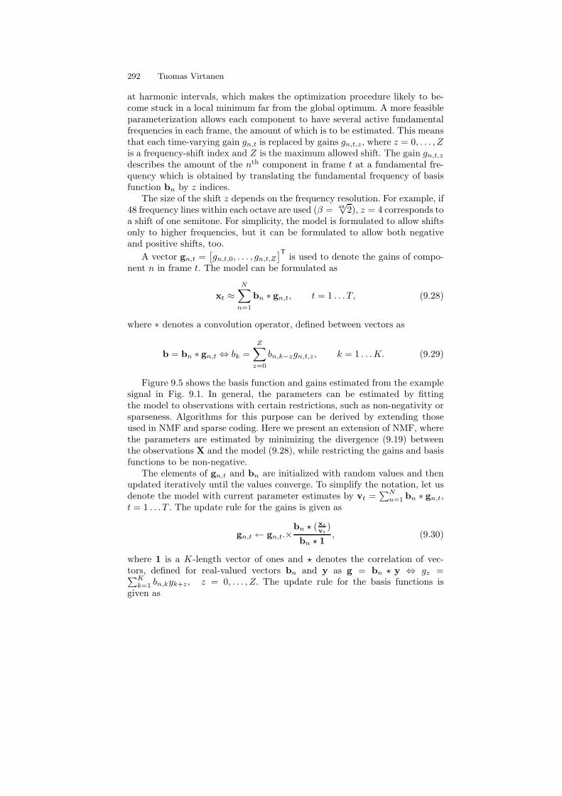
Figure 9.5 shows the basis function and gains estimated from the examplesignal in Fig. 9.1. In general, the parameters can be estimated by fittingthe model to observations with certain restrictions, such as non-negativity orsparseness. Algorithms for this purpose can be derived by extending thoseused in NMF and sparse coding. Here we present an extension of NMF, wherethe parameters are estimated by minimizing the divergence (9.19) betweenthe observations X and the model (9.28), while restricting the gains and basisfunctions to be non-negative.

The elements of gn,t and bn are initialized with random values and thenupdated iteratively until the values converge. To simplify the notation, let usdenote the model with current parameter estimates by vt =

∑N

n=1bn ∗ gn,t,

t = 1 . . . T . The update rule for the gains is given as

gn,t ← gn,t.×bn ⋆ (xt

vt

)

bn ⋆ 1, (9.30)

where 1 is a K-length vector of ones and ⋆ denotes the correlation of vec-tors, defined for real-valued vectors bn and y as g = bn ⋆ y ⇔ gz =∑K

k=1bn,kyk+z, z = 0, . . . , Z. The update rule for the basis functions is

given as


bn ← bn.×∑T

t=1(gn,t ⋆ xt

vt

)

gn,t ⋆ 1. (9.31)

The overall optimization algorithm for non-negative matrix deconvolutionis as follows:

Algorithm 9.2: Non-Negative Matrix Deconvolution

1. Initialize each gn,t and bn with the absolute values of Gaussian noise.2. Calculate vt =

N

n=1bn ∗ gn,t for each t = 1 . . . T .

3. Update each gn,t using (9.30).4. Calculate vt as in Step 2.5. Update each bn using (9.31). Repeat Steps (2)–(5) until the values converge.

The algorithm produces good results if the number of sources is small, butfor multiple sources and more complex signals, it is difficult to get as good

Time (seconds)

Fu

nd

am

en

tal fr

eq

ue

ncy s

hift

(qu

art

er

se

mito

ne

s)

0 1 2 3

0

10

20

30

40

50

102

104

−50

−40

−30

−20

−10

0

10

Frequency (Hertz)

Am

plit

ud

e (

dB

)

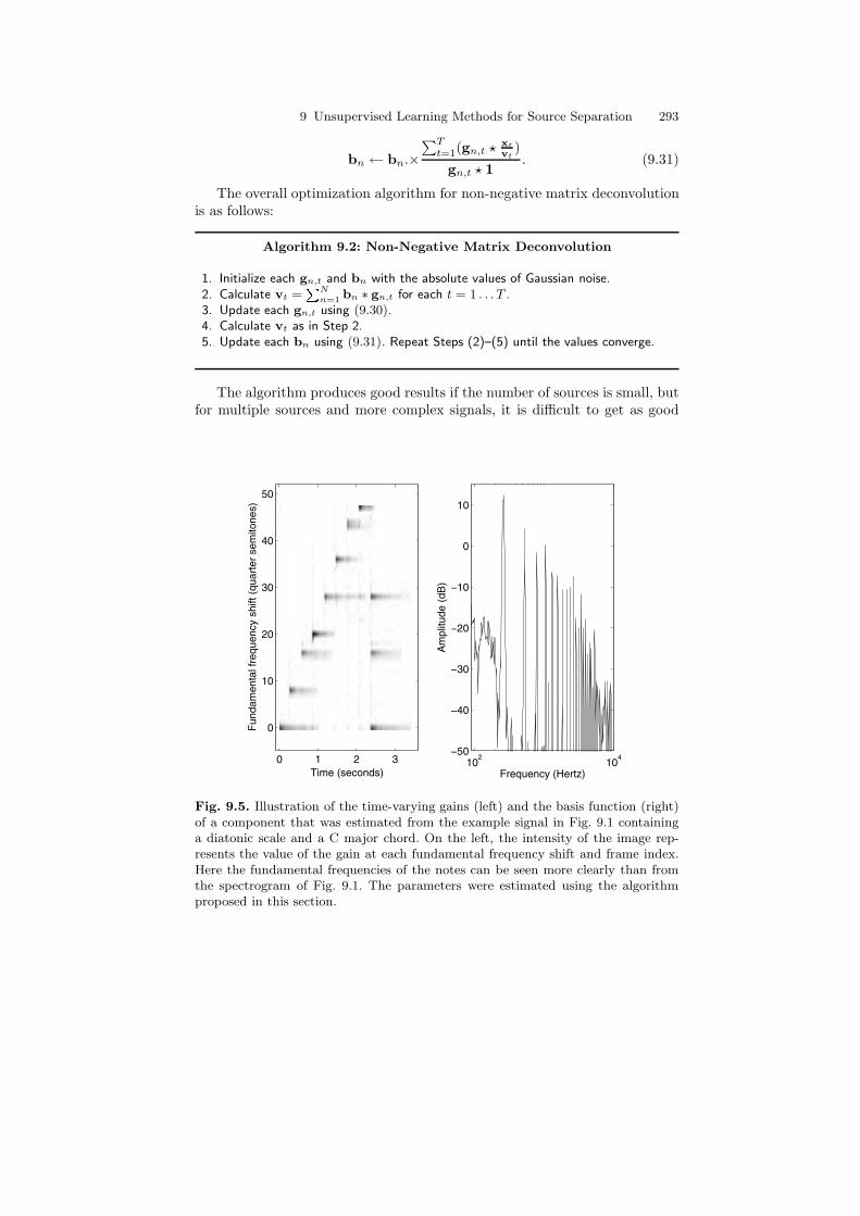
Fig. 9.5. Illustration of the time-varying gains (left) and the basis function (right)of a component that was estimated from the example signal in Fig. 9.1 containinga diatonic scale and a C major chord. On the left, the intensity of the image rep-resents the value of the gain at each fundamental frequency shift and frame index.Here the fundamental frequencies of the notes can be seen more clearly than fromthe spectrogram of Fig. 9.1. The parameters were estimated using the algorithmproposed in this section.

294 Tuomas Virtanen

results as those illustrated in Fig. 9.5. The model allows all the fundamentalfrequencies within the range z = 0 . . . Z to be active simultaneously, thus, it isnot restrictive enough. For example, the algorithm may model a non-harmonicdrum spectrum by using a harmonic basis function shifted to multiple adjacentfundamental frequencies. Ideally, this could be solved by restricting the gainsto be sparse, but the sparseness criterion complicates the optimization.

In principle, it is possible to combine time-varying spectra and time-varying fundamental frequencies into the same model, but this further in-creases the number of free parameters so that it can be difficult to obtaingood separation results.

When shifting the harmonic structure of the spectrum, the formant struc-ture becomes shifted, too. Therefore, representing time-varying pitch by trans-lating the basis function is appropriate only for nearby pitch values. It isunlikely that the whole fundamental frequency range of an instrument couldbe modelled by shifting a single basis function.

9.9 Evaluation of the Separation Quality

A necessary condition for the development of source separation methods isthe ability to measure the quality of their results. In general, the separationquality can be measured by calculating the error between the separated sig-nals and reference sources, or by listening to the separated signals. In the casethat separation is used as a pre-processing step for automatic music tran-scription, the quality should be judged according to the final application, i.e.,the transcription accuracy.

Performance measures for audio source separation tasks have been dis-cussed, e.g., by Gribonval et al. [258]. They proposed measures estimating theamount of interference from other sources and the distortion caused by theseparation algorithm. Many authors have used the signal-to-distortion ratio

(SDR) as a simple measure to summarize the quality. This is defined in deci-bels as

SDR [dB] = 10 log10

∑

t s(t)2∑

t[s(t) − s(t)]2, (9.32)

where s(t) is a reference signal of the source before mixing, and s(t) is the sep-arated signal. In the separation of music signals, Jang and Lee [314] reportedaverage SDR of 9.6 dB for an ISA-based algorithm which trains basis func-tions separately for each source. Helen and Virtanen [282] reported averageSDR of 6.4 dB for NMF in the separation of drums and polyphonic harmonictrack, and a clearly lower performance (SDR below 0 dB) for ISA.

In practice, quantitative evaluation of the separation quality requires thatreference signals, i.e., the original signals s(t) before mixing, be available. Inthe case of real-world music signals, it is difficult to obtain the tracks of eachindividual source instrument and, therefore, synthesized material is often used.


Generating test signals for this purpose is not a trivial task. For example, ma-terial generated using a software synthesizer may produce misleading resultsfor algorithms which learn structures from the data, since many synthesiz-ers produces notes which are identical at each repetition. In the case thatsource separation is a part of a music transcription system, quality evaluationrequires that audio signals with an accurate reference notation are available(see Chapter 11, p. 355). Large-scale comparisons of different separation al-gorithms for music transcription have not been made.

9.10 Summary and Discussion

The algorithms presented in this chapter show that rather simple principlescan be used to learn and separate sources from music signals in an unsuper-vised manner. Individual musical sounds can usually be modelled quite wellusing a fixed spectrum with time-varying gain, which enables the use of ICA,sparse coding, and NMF algorithms for their separation. Actually, all the al-gorithms based on the linear model (9.4) can be viewed as performing matrixfactorization; the factorization criteria are just different.

The simplicity of the additive model makes it relatively easy to extendand modify it, along with the presented algorithms. However, a challengewith the presented methods is that it is difficult to incorporate some types ofrestrictions for the sources. For example, it is difficult to restrict the sourcesto be harmonic if they are learned from the mixture signal.

Compared to other approaches towards monaural sound source separa-tion, the unsupervised methods discussed in this chapter enable a relativelygood separation quality—although it should be noted that the performancein general is still very limited. A strength of the presented methods is theirscalability: the methods can be used for arbitrarily complex material. In thecase of simple monophonic signals, they can be used to separate individualnotes, and in complex polyphonic material, the algorithms can extract largerrepeating entities, such as chords. Some of the algorithms, for example NMFusing the magnitude spectrogram representation, are quite easy to imple-ment. The computational complexity of the presented methods may restricttheir applicability if the number of components is large or the target signal islong.

Large-scale evaluations of the described algorithms on real-world poly-phonic music recordings have not been presented. Most published results usea small set of test material and the results are not comparable with eachother. Although conclusive evaluation data are not available, a preliminaryexperience from our simulations has been that NMF (or sparse coding withnon-negativity restrictions) often produces better results than ISA. It wasalso noticed that prior information about sources can improve the separationquality significantly. Incorporating higher-level models into the optimization

296 Tuomas Virtanen

algorithms is a big challenge, but will presumably lead to better results. Con-trary to the general view held by most researchers less than 10 years ago,unsupervised learning has proven to be applicable for the analysis of real-world music signals, and the area is still developing rapidly.

Documents

9 Unsupervised Learning Methods for Source Separation · PDF file9 Unsupervised Learning Methods for Source Separation in Monaural Music Signals Tuomas Virtanen Institute of Signal