8-hr Ozone National Ambient Air Quality Standard (NAAQS

8-hr Ozone National Ambient Air Quality Standard (NAAQS)

Implementation

EPAJuly 2, 2002

Pilat Edited

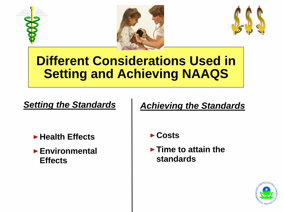
Different Considerations Used in Setting and Achieving NAAQS

Achieving the StandardsSetting the Standards

CostsTime to attain the standards

Health EffectsEnvironmental Effects

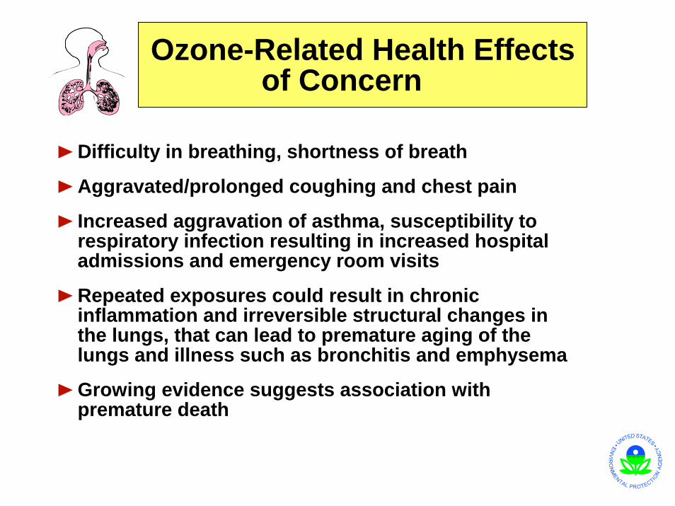
Difficulty in breathing, shortness of breath

Aggravated/prolonged coughing and chest pain

Increased aggravation of asthma, susceptibility to respiratory infection resulting in increased hospital admissions and emergency room visits

Repeated exposures could result in chronic inflammation and irreversible structural changes in the lungs, that can lead to premature aging of the lungs and illness such as bronchitis and emphysema

Growing evidence suggests association with premature death

Ozone-Related Health Effects of Concern

What is the New 8-Hour Ozone NAAQS?

The New Ozone NAAQS is an 8-hour standard at the level of 0.08 ppm (parts per million by gaseous volume) with a form based on the 3-year average of the annual 4th highest daily maximum 8-hour average Ozone concentrations measured at each ozone monitor within a geographical area.Pilat Comment: Note that if there are no ozone monitoring instruments, Ozone NAAQS will not be exceeded. Hence some regions avoid installing ozone monitors.

O3 NAAQS

Averaging Time 1-hr NAAQS 8-hr NAAQSAvg time 1-hour 8-hourLevel 0.12 ppm 0.08 ppmForm exceedance-based concentration-basedAir Quality Indicator daily max 1-hr conc within

daydaily max 8-hr conc starting within day

NAAQS Statistic annual estimated exceedances

annual 4th high 8-hr daily max conc

Rounding 0.125 ppm--smallest number greater than the 0.12 ppm NAAQS level

0.085 ppm--smallest number greater than 0.08 ppm NAAQS level

Compliance period three consecutive years three consecutive yearsAttainment Test avg expected exceed'c rate

<= 1.0 avg annual 4th high daily max 8-hour conc <= 0.08 ppm

12 1 12

8

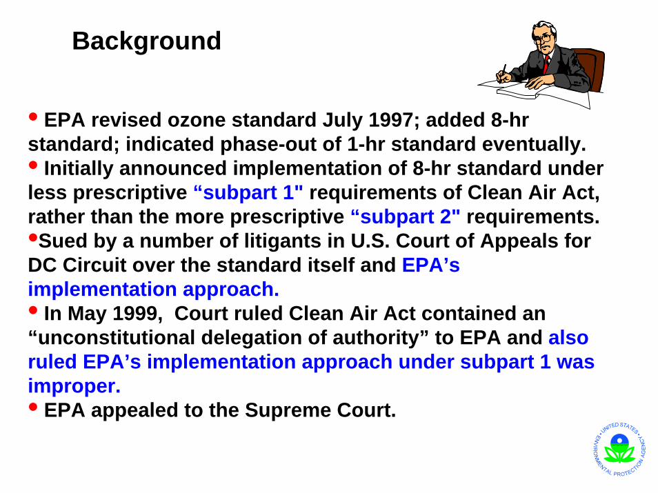
• EPA revised ozone standard July 1997; added 8-hr standard; indicated phase-out of 1-hr standard eventually.• Initially announced implementation of 8-hr standard under less prescriptive “subpart 1" requirements of Clean Air Act, rather than the more prescriptive “subpart 2" requirements.•Sued by a number of litigants in U.S. Court of Appeals for DC Circuit over the standard itself and EPA’s implementation approach.• In May 1999, Court ruled Clean Air Act contained an “unconstitutional delegation of authority” to EPA and also ruled EPA’s implementation approach under subpart 1 was improper.• EPA appealed to the Supreme Court.

Background

• In February 2001, Supreme Court upheld constitutionality of the standard-setting process in the Clean Air Act, but ruled that EPA’s implementation approach was unlawful and that EPA could not ignore subpart 2 when implementing the 8-hr standard.

• Supreme Court recognized gaps in the subpart 2 scheme, however, and left it to EPA to develop a reasonable resolution of the roles of subparts 1 and 2 in implementing a revised ozone standard.

• Court said …“It may well be ... that some provisions of Subpart 2 are ill fitted to implementation of the revised standard.”

More from the Supreme Court decision …

Background (continued)

Currently revising options for addressing Supreme Court rulingand for other implementation issues.

Taking input from stakeholders and the public at large from public meetings & written comments.

(Note these slides presented in July 2002)

Background (continued)

what areas of the country exceed the 8-hr standards?

Provide incentives for expeditious attainment of O3 8-hour standard … avoid incentives for delay to protect public health.• Provide reasonable attainment deadlines.• Have a basic, straightforward structure that can be communicated easily.• Consistent with Clean Air Act and US Supreme Court decision, provide flexibility to states and EPA on implementation approaches and control measures• Emphasize national and regional measures to help areas come into attainment and, where possible, reduce the need for more expensive local controls.• Provide a smooth transition from 1-hr O3 NAAQS to 8-hr O3NAAQS implementation

Principles Guiding EPA When Developing Approach to Meet O3 NAAQS

• Propose rulemaking on the implementation approach in summer of 2002 … finalize the rule in mid-2003.

•During 2003 …. ask State/Tribes to update recommended designations … promulgate air quality designations in mid-2004.

• State implementation plans (SIPs) …. likely be due in the 2007 and 2008 time frame, with attainment dates ranging from 2007 to 2019 or longer.

• No plans for EPA to issue final designations of nonattainment areas until EPA issues a final implementation strategy for the O3 standard.

Schedule

UnderSubpart 1

UnderSubpart 2 Action

2003

2004

2005

2007

2007-2008

2007

2009*

Same

Same

Same

Same

Same

2007*

2010*

2013*

2019-2021*

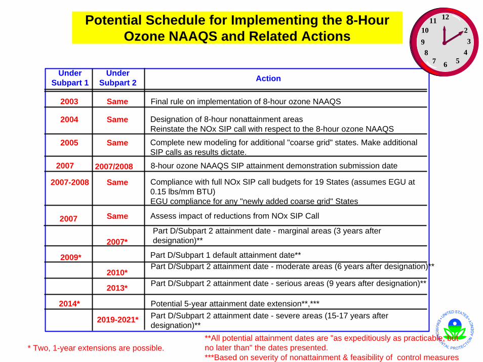
Final rule on implementation of 8-hour ozone NAAQS

Designation of 8-hour nonattainment areasReinstate the NOx SIP call with respect to the 8-hour ozone NAAQS

Complete new modeling for additional "coarse grid" states. Make additional SIP calls as results dictate.

8-hour ozone NAAQS SIP attainment demonstration submission date

Compliance with full NOx SIP call budgets for 19 States (assumes EGU at 0.15 lbs/mm BTU)EGU compliance for any "newly added coarse grid" States

Assess impact of reductions from NOx SIP Call

Part D/Subpart 2 attainment date - marginal areas (3 years after designation)**

Part D/Subpart 1 default attainment date**Part D/Subpart 2 attainment date - moderate areas (6 years after designation)**

Part D/Subpart 2 attainment date - serious areas (9 years after designation)**

Potential 5-year attainment date extension**,***Part D/Subpart 2 attainment date - severe areas (15-17 years after designation)**

2007/2008

2014*

Potential Schedule for Implementing the 8-Hour Ozone NAAQS and Related Actions

* Two, 1-year extensions are possible.**All potential attainment dates are "as expeditiously as practicable, but no later than" the dates presented. ***Based on severity of nonattainment & feasibility of control measures

12

23

4567

8910

11

Where EPA Is (July 2002)

• Assessing comments from the public meetings & written comments

• Revising some options, considering new ones

• Starting to develop Federal Register proposed rule notice—planning to propose several alternative approaches

http://www.epa.gov/ttn/rto/ozonetech/o3imp8hr/o3imp8hr.htm

Information on the Web including comments received ….

• Photochemical smog– How it forms, key ingredients

• Photolysis– Photolytic cycle

• Role of reactive organics RO2• Control of smog• EKMA or Empirical Kinetic

Modeling Approach (note an EKMA graph enables the estimation of the NOxand VOC emission reduction needed to meet O3 air quality standard)

• What are the essential ingredients for creating

photochemical smog?Nitrogen oxides NOx , sun,

reactive organics RO2

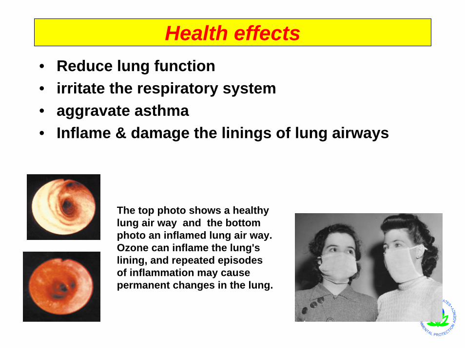
Health effects• Reduce lung function• irritate the respiratory system• aggravate asthma• Inflame & damage the linings of lung airways

The top photo shows a healthy lung air way and the bottom photo an inflamed lung air way. Ozone can inflame the lung's lining, and repeated episodes of inflammation may cause permanent changes in the lung.

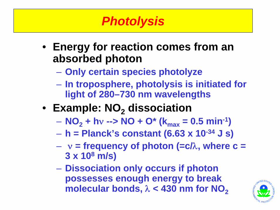
Photolysis

• Energy for reaction comes from an absorbed photon– Only certain species photolyze– In troposphere, photolysis is initiated for

light of 280–730 nm wavelengths• Example: NO2 dissociation

– NO2 + hν --> NO + O* (kmax = 0.5 min-1)– h = Planck’s constant (6.63 x 10-34 J s) – ν = frequency of photon (=c/λ, where c =

3 x 108 m/s)– Dissociation only occurs if photon

possesses enough energy to break molecular bonds, λ < 430 nm for NO2

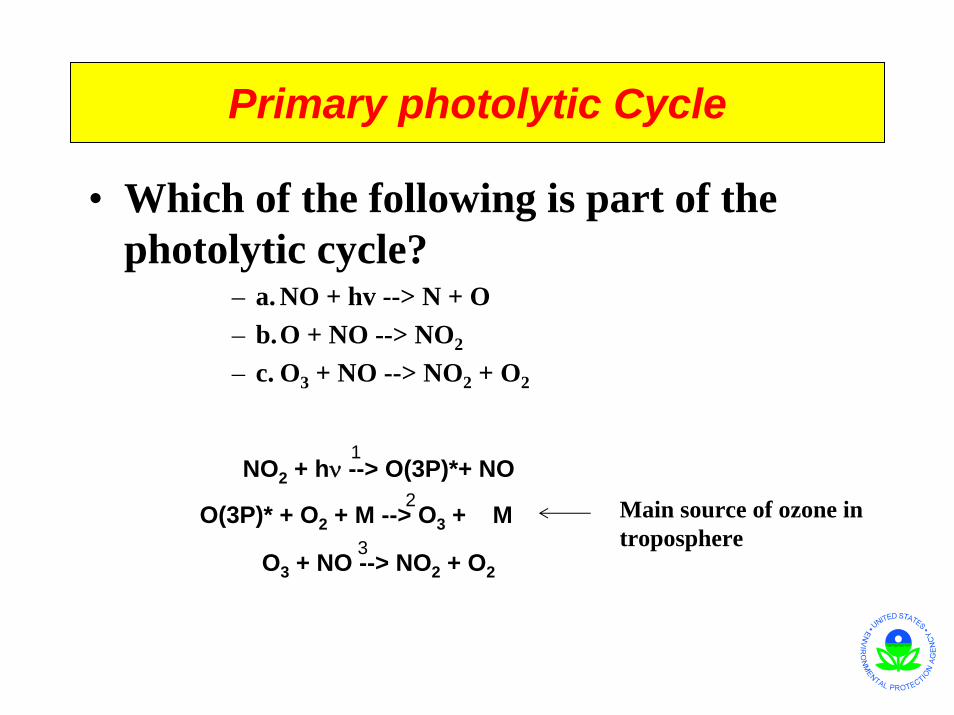
Primary photolytic Cycle

• Which of the following is part of the photolytic cycle?

– a. NO + hv --> N + O– b.O + NO --> NO2

– c. O3 + NO --> NO2 + O2

NO2 + hν --> O(3P)*+ NO

O(3P)* + O2 + M --> O3 + M

O3 + NO --> NO2 + O2

1

2

3

Main source of ozone in troposphere

Ozone is higher than photolytic reactions predict!

• Assuming photostationary state for O and O3, then we can derive equation for O3

formation:

• When NO2 ~ NO, ozone is predicted by above to be around 20 ppb

• But in reality ozone concentration is much higher by as much as an order of magnitude -

O3[ ]=k1 NO2[ ]k3 NO[ ]

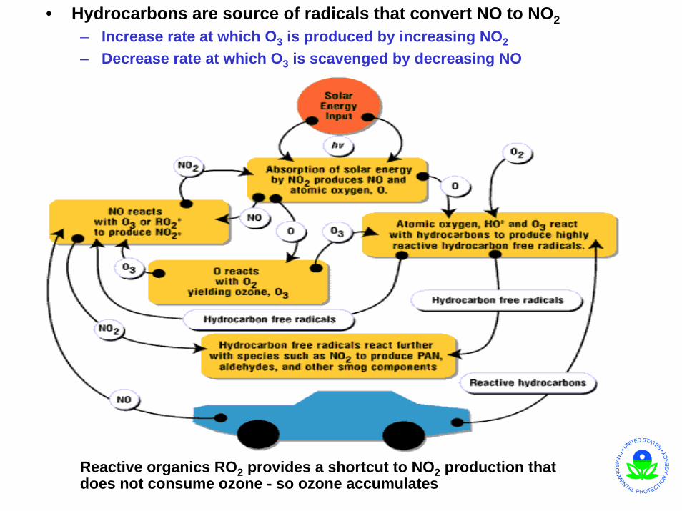
• Hydrocarbons are source of radicals that convert NO to NO2– Increase rate at which O3 is produced by increasing NO2

– Decrease rate at which O3 is scavenged by decreasing NO

O3

NO2

O

NO

O2 & M

hν

RO2

Reactive organics RO2 provides a shortcut to NO2 production that does not consume ozone - so ozone accumulates

Control of Ozone Smog• Ozone smog is a Secondary air pollutant • Must control primary emissions of O3precursors to control smog: HCs, NOx

– source of HCs: solvents, cars, trucks, industrial sources

– source of NOx: cars, trucks, all combustion, power plants,

– Analyze system using EPA’s EKMA or Empirical Kinetic Modeling Approach

– Relates changes in HCs and NOx emissions to changes in maximum ozone concentration

– EKMA diagram can be used to estimate reductions in HCs and NOx concentrations in air needed to reduce ozone air concentrations to NAAQS.

Weekend/Weekday Ozone Observationsin the South Coast Air Basin

Sponsored by

National Renewable Energy Laboratory and Coordinating Research Council

Eric Fujita, Robert Keislar, and William StockwellDesert Research Institute

University and Community College System of NevadaReno, Nevada

Paul Roberts, Hilary Main, and Lyle ChinkinSonoma Technology, Inc.

Petaluma, CA

Weekend/Weekday Ozone Effect WorkshopSacramento, CA

November 16, 1999

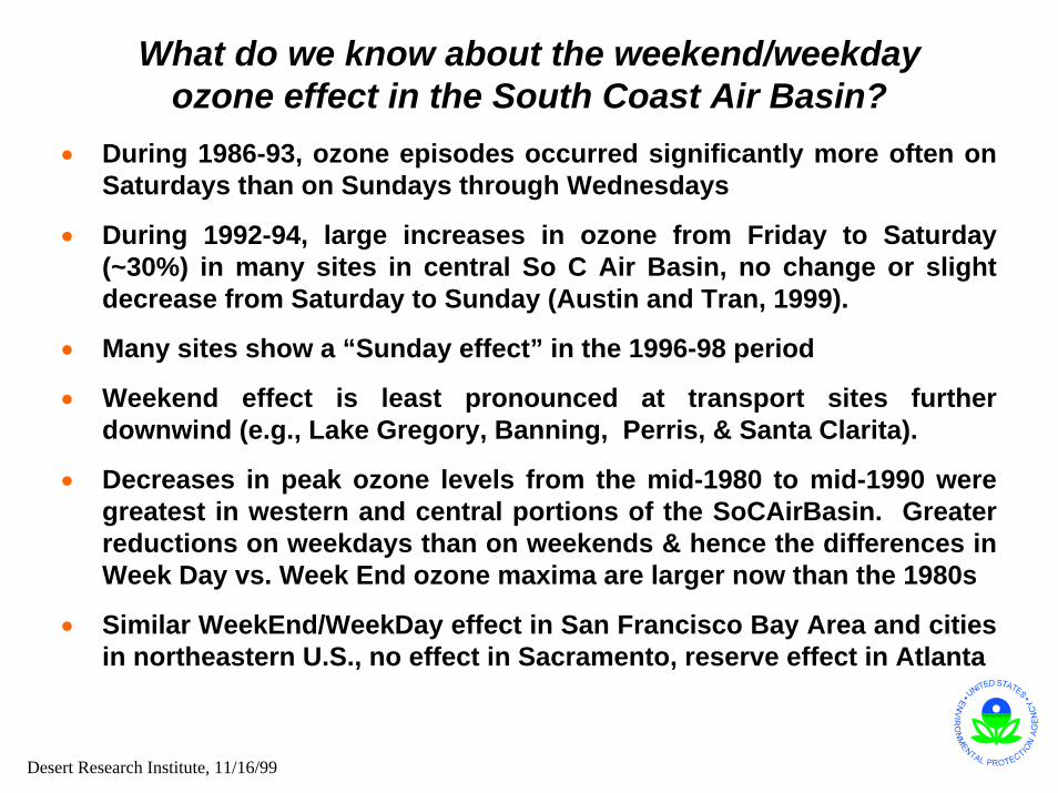
What do we know about the weekend/weekday ozone effect in the South Coast Air Basin?

• During 1986-93, ozone episodes occurred significantly more often on Saturdays than on Sundays through Wednesdays

• During 1992-94, large increases in ozone from Friday to Saturday (~30%) in many sites in central So C Air Basin, no change or slight decrease from Saturday to Sunday (Austin and Tran, 1999).

• Many sites show a “Sunday effect” in the 1996-98 period

• Weekend effect is least pronounced at transport sites further downwind (e.g., Lake Gregory, Banning, Perris, & Santa Clarita).

• Decreases in peak ozone levels from the mid-1980 to mid-1990 were greatest in western and central portions of the SoCAirBasin. Greater reductions on weekdays than on weekends & hence the differences in Week Day vs. Week End ozone maxima are larger now than the 1980s

• Similar WeekEnd/WeekDay effect in San Francisco Bay Area and cities in northeastern U.S., no effect in Sacramento, reserve effect in Atlanta

Desert Research Institute, 11/16/99

What do we know about the weekend/weekday differences in VOC, NOx and PM in the South Coast Air Basin?

• VOC, NOx and PM are all higher during weekdays.

• During 1986-93, average early morning NO2 and NOx were lower by 20-25% and 30-50%, respectively on weekend days in the Coastal/Metropolitan region of the SoCAB. (Blier and Winer, 1996)

• Morning NOx is highest on weekdays, followed by Sat and lowest on Sunday.

• Sat afternoon levels are comparable to or slightly lower than weekday levels.

• Saturday evening levels tend to be lower than on Friday and roughly equal to or higher than the mean weekday evening levels.

• NOx mixing ratios are lower on Sunday than other days for all hours except at midnight to 4 a.m. when they are comparable to weekdays.

• The reactivity of the ambient hydrocarbon mixture has dropped between 1995 and 1996. Reactivity appears slightly lower on weekends (Franzwaand Pasek, 1999).

• 6 to 9 a.m.VOC/NOx ratios have decreased from 8 to 10 in 1987 (SCAQS) to 4 to 7 in 1997.


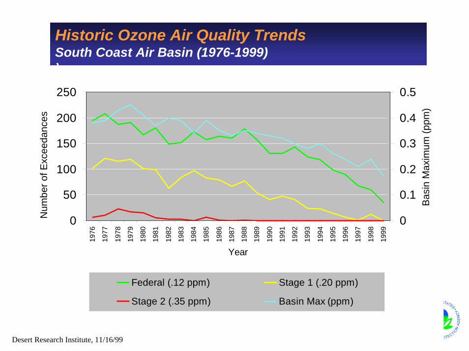
Historic Ozone Air Quality TrendsSouth Coast Air Basin (1976-1999))

0

50

100

150

200

25019

76

1977

1978

1979

1980

1981

1982

1983

1984

1985

1986

1987

1988

1989

1990

1991

1992

1993

1994

1995

1996

1997

1998

1999

Year

Num

ber o

f Exc

eeda

nces

0

0.1

0.2

0.3

0.4

0.5

Bas

in M

axim

um (p

pm)

Federal (.12 ppm) Stage 1 (.20 ppm)

Stage 2 (.35 ppm) Basin Max (ppm)


Historic Ozone Air Quality TrendsSouth Coast Air Basin (1980-1997) - CENTRAL

0

0.1

0.2

0.3

0.4

0.5

0.619

80

1981

1982

1983

1984

1985

1986

1987

1988

1989

1990

1991

1992

1993

1994

1995

1996

1997

Year

Ave

rage

max

1-h

r Ozo

ne (p

pm)

Azusa Glendora Pomona Upland


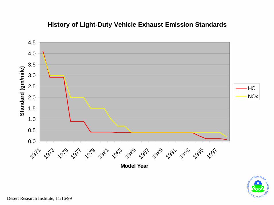
History of Light-Duty Vehicle Exhaust Emission Standards

0.0

0.5

1.0

1.5

2.0

2.5

3.0

3.5

4.0

4.5

1971

1973

1975

1977

1979

1981

1983

1985

1987

1989

1991

1993

1995

1997

Model Year

Stan

dard

(gm

/mile

)

HCNOx


Ozone (ppb)

400360

120

160

200

28080

2.0 2.2 2.4 2.6 2.8 3.0 3.2 3.4

2.8

2.6

2.4

2.2

2.0

1.8

1.6

1.4

1.2

1.0

0.8

1997

19871992

log

NO

x (p

pb)

log VOC (ppbC)

Ozone EKMA Plot (ppb)RADM2 Mechanism

Average VOC and NOx at Azusa

Ozone (ppb)

2.0 2.2 2.4 2.6 2.8 3.0 3.2 3.4

2.8

2.6

2.4

2.2

2.0

1.8

1.6

1.4

1.2

1.0

0.8

1997

19871992

log

NO

x (p

pb)

log VOC (ppbC)

St k ll d F jit P t b S b itt d

Average VOC and NOx at Azusa

10.012.5

7.5

5.0

2.5

15.0

VOC/NOx Contour and O3 EKMA Plot (Color) RADM2 Mechanism

0

200

400

600800

1000

0

20

40

60

80

100

0

40

80

120

160

200

240

MaximumOzone (ppb)

InitialVOC (ppbC)

InitialNOx (ppb)

3D EKMA

Factors Affecting the Magnitude and Spatial Extent of the Week End/Week Day Ozone Effect

• Ozone formation depends on VOC, NOx and VOC/NOx ratios .– For VOC/NOx < 5.5, OH reacts more with NO2, removing radicals and NOx to retard O3 formation. Under

these conditions, a decrease in NOx favors O3 formation. – At low NOx mixing ratios, or sufficiently high VOC/NOx, decrease in NOx favors peroxy-peroxy

reactions, which retard O3 formation by removing free radicals from the system. – At a given level of VOC, there exists an optimum VOC/NOx ratio at which a maximum amount of ozone is

produced. For ratios less than this optimum ratio, increasing NOx decreases ozone. This situation occurs more commonly in urban centers and is the case for most of the central SoCAB.

• Week End/Week Day differences in VOC and NOx emissions patterns (Diurnal and Spatial Distribution).

• Transport and– Increasing mixing height due to surface heating reduces [VOC] and [NOx]. – Horizontal transport increases VOC/NOx ratios due to more rapid removal of NOx than

VOC.

The observed "weekend effect" in the South Coast Air Basin arises from differences in ozone forming potential due to day-of-the-week changes in ROG and NOx emissions. Variations in meteorology affect the magnitude

and spatial extent of the WE/WD ozone effect within the basin.


Preliminary Hypotheses1. Ozone formation in SoCalif Air Basin, particularly the western & central portions

of the basin, is VOC-sensitive with respect to O3 formation. VOC/NOx ratios are higher on weekends due to Week End/Week Day changes in emissions resulting in greater O3 forming potential despite lower [VOC] and [NOx] on weekends.

– The weekend effect is greater where Δ [O3]max/Δ[VOC] is greater during weekdays than during weekend days.

– Week End/Week Day effect is most pronounced in area of the basin with the greatest NOx disbenefit (i.e., most VOC-limited on weekdays).

2. The magnitude of the weekend effect is a function of the O3 forming potential and the time available for O3 formation before dilution offsets O3 formation.

3. The "weekend effect" is less pronounced in the eastern portion of the SoCAirBwhere Week End/Week Day differences in VOC and NOx emissions are masked by emission transport. Transport causes higher VOC/NOx ratios due to more rapid removal of NOx versus VOC as the emissions are transported toward the eastern side of the Basin.

4. Overnight carry-over of O3, VOC and NOx from Friday and Saturday nights are greater than during other days of the week. Increased carryover is greater for VOC than for NOx. This affects the O3 forming potential of the ambient air.


Global Models Of Atmospheric Composition

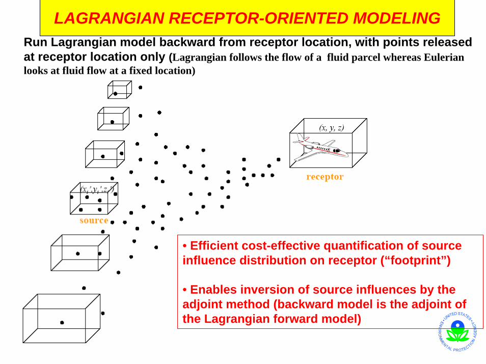
LAGRANGIAN RECEPTOR-ORIENTED MODELINGRun Lagrangian model backward from receptor location, with points released at receptor location only (Lagrangian follows the flow of a fluid parcel whereas Eulerianlooks at fluid flow at a fixed location)

• Efficient cost-effective quantification of source influence distribution on receptor (“footprint”)

• Enables inversion of source influences by the adjoint method (backward model is the adjoint of the Lagrangian forward model)

Embedding Lagrangian Plumes in Eulerian Models

Release puffs from point sources and transport them along trajectories, allowing them to gradually dilute by turbulent mixing (“Gaussian plume”) until they reach the Eulerian grid size at which point they mix into the gridbox

• Advantages: resolve subgrid ‘hot spots’ and associated nonlinear processes (chemistry, aerosol growth) within plume• Difference with Lagrangian approach is that (1) puff has volume as well as mass, (2) turbulence is deterministic (Gaussian spread) rather than stochastic

S. California fire plumes,Oct. 25 2004

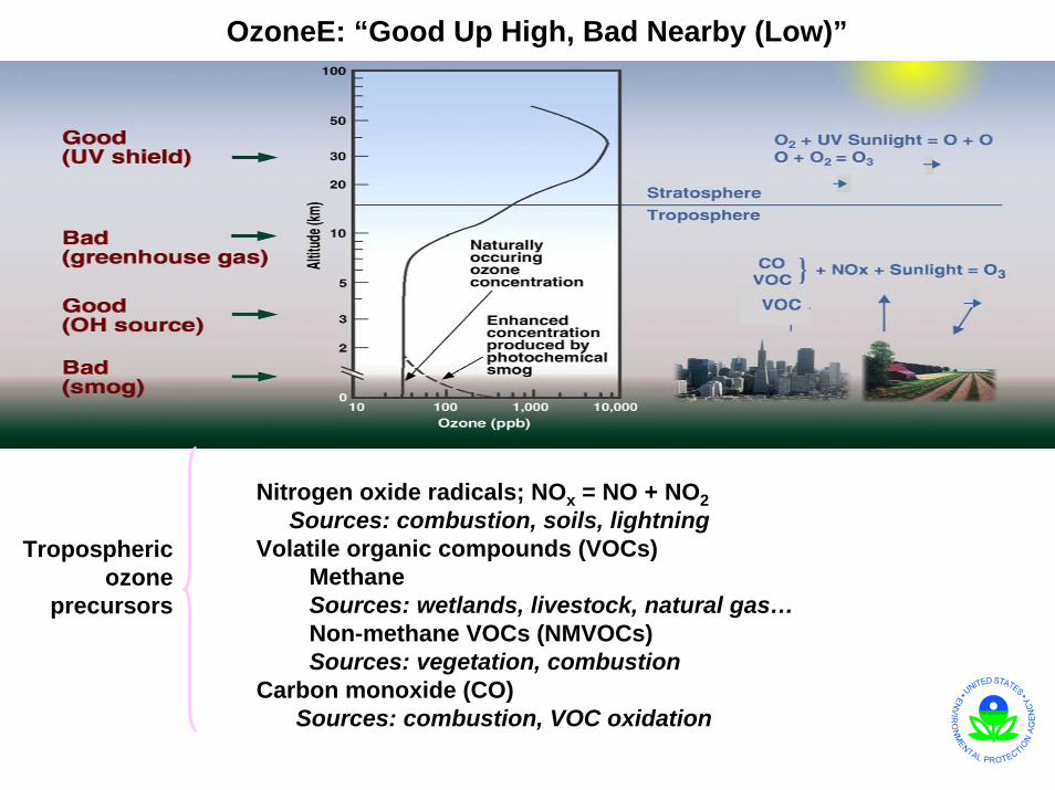
OzoneE: “Good Up High, Bad Nearby (Low)”

Nitrogen oxide radicals; NOx = NO + NO2Sources: combustion, soils, lightning

Volatile organic compounds (VOCs)MethaneSources: wetlands, livestock, natural gas…Non-methane VOCs (NMVOCs)Sources: vegetation, combustion

Carbon monoxide (CO)Sources: combustion, VOC oxidation

Troposphericozone

precursors

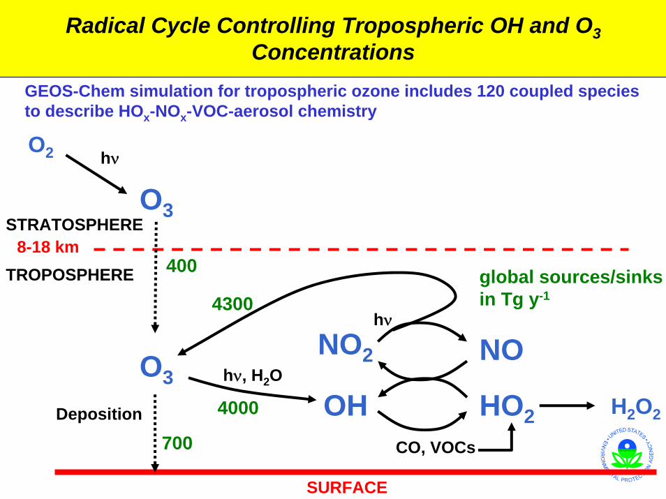
Radical Cycle Controlling Tropospheric OH and O3Concentrations

O3

O2 hν

O3OH HO2

hν, H2O

Deposition

NO

H2O2

CO, VOCs

NO2

hν

STRATOSPHERE

TROPOSPHERE8-18 km

SURFACE

GEOS-Chem simulation for tropospheric ozone includes 120 coupled speciesto describe HOx-NOx-VOC-aerosol chemistry

global sources/sinksin Tg y-14300

4000

400

700

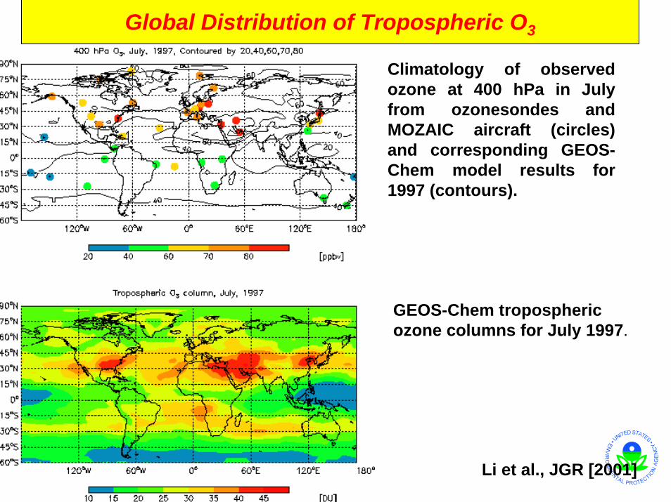
Climatology of observed ozone at 400 hPa in July from ozonesondes and MOZAIC aircraft (circles) and corresponding GEOS-Chem model results for 1997 (contours).

GEOS-Chem tropospheric ozone columns for July 1997.

Global Distribution of Tropospheric O3

Li et al., JGR [2001]

Global Distribution of Tropospheric O3

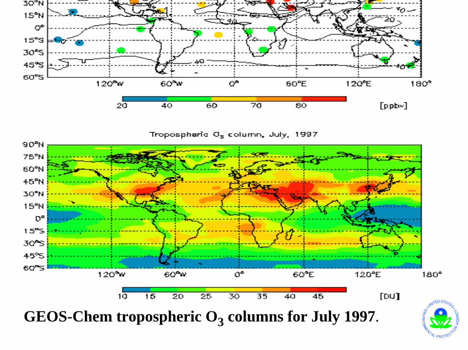
GEOS-Chem tropospheric O3 columns for July 1997.

COMPARISON TO TES SATELLITE OBSERVATIONS IN MIDDLE TROPOSPHERE

Zhang et al. [2006]

averagingkernels

(July 2005)

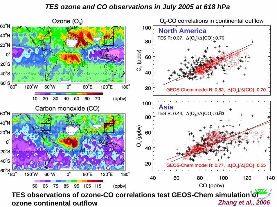
TES ozone and CO observations in July 2005 at 618 hPa

TES observations of ozone-CO correlations test GEOS-Chem simulation of ozone continental outflow

North America

Asia

Zhang et al., 2006

IPCC Radiative Forcing Estimate For Tropospheric Ozone (0.35 W m-2)Relies on Global Models

Preindustrialozone models

}Observations at mountain sites in Europe [Marenco et al., 1994]

…but these underestimate the observed rise in ozone over the 20th century

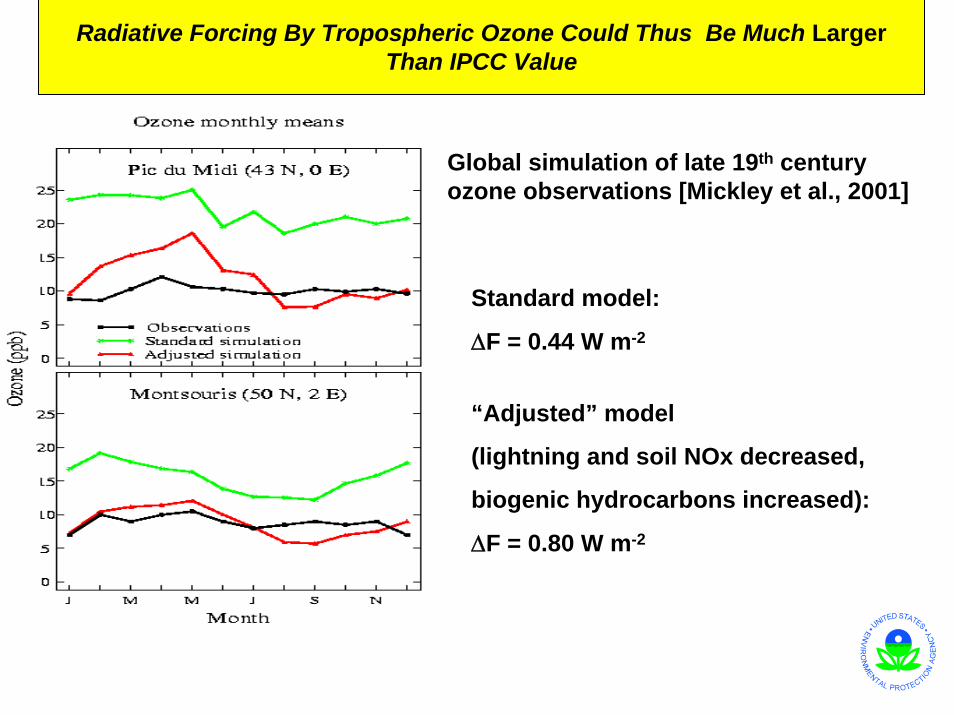
Radiative Forcing By Tropospheric Ozone Could Thus Be Much Larger Than IPCC Value

Standard model:

ΔF = 0.44 W m-2

“Adjusted” model

(lightning and soil NOx decreased,

biogenic hydrocarbons increased):

ΔF = 0.80 W m-2

Global simulation of late 19th century ozone observations [Mickley et al., 2001]

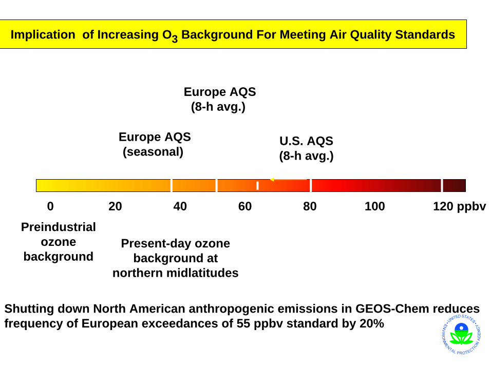
Implication of Increasing O3 Background For Meeting Air Quality Standards

0 20 40 60 80 100 120 ppbv

Europe AQS(seasonal)

U.S. AQS(8-h avg.)

U.S. AQS(1-h avg.)

Preindustrialozone

backgroundPresent-day ozone

background at northern midlatitudes

Europe AQS(8-h avg.)

Shutting down North American anthropogenic emissions in GEOS-Chem reduces frequency of European exceedances of 55 ppbv standard by 20%

U.S. EPA defines a “policy-relevant background” (PRB) as the O3 concentration that would be present in U.S. surface air in the

absence of North American anthropogenic emissions

(1) Standard simulation; include all sources

(2) Set U.S. or N. American anthropogenic emissions to zero infer policy-relevant background

(3) Set global anthropogenic emissions to zero estimate natural background

Difference between (1) and (2) regional pollution

Difference between (2) and (3) background enhancement from hemispheric pollution

• This O3 background cannot be directly observed, must be estimated from models• Because chemistry is strongly nonlinear, sensitivity simulations are necessary

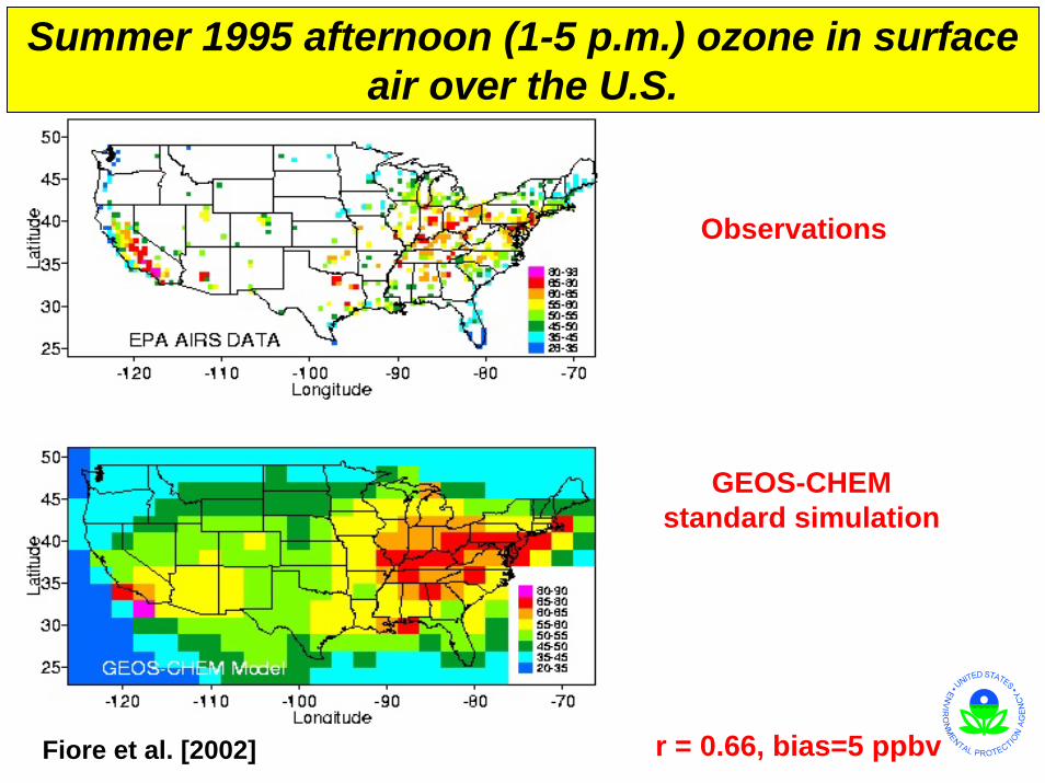
Summer 1995 afternoon (1-5 p.m.) ozone in surface air over the U.S.

Observations

r = 0.66, bias=5 ppbv

GEOS-CHEMstandard simulation

Fiore et al. [2002]

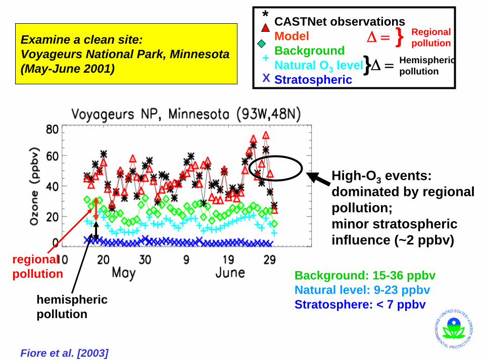
Examine a clean site: Voyageurs National Park, Minnesota(May-June 2001)

CASTNet observationsModelBackgroundNatural O3 levelStratospheric

+

*

Hemisphericpollution

Regionalpollution}Δ =

}Δ =

Background: 15-36 ppbvNatural level: 9-23 ppbvStratosphere: < 7 ppbv

High-O3 events: dominated by regional pollution; minor stratospheric influence (~2 ppbv)

regional pollution

hemispheric pollution

X

Fiore et al. [2003]

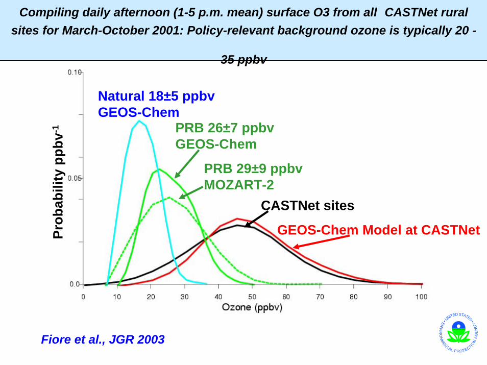
Compiling daily afternoon (1-5 p.m. mean) surface O3 from all CASTNet rural sites for March-October 2001: Policy-relevant background ozone is typically 20 -

35 ppbvPr

obab

ility

ppb

v-1

CASTNet sites

GEOS-Chem Model at CASTNet

Natural 18±5 ppbvGEOS-Chem

PRB 26±7 ppbvGEOS-Chem

PRB 29±9 ppbvMOZART-2

Fiore et al., JGR 2003

EFFECT OF 2000-2050 Climate Change on U.S. Ozone Pollution

2000 2050 climate - 2000

Wu et al. [2007]

Run GEOS-Chem driven by GISS GCM for present vs. 2050 climate

Climate change decreases the background ozone because higher water vapor increases ozone loss;

but water vapor aggravates ozone pollution episodes due to less ventilation (fewer mid-latitudes cyclones), faster chemistry, higher biogenic VOC emissions

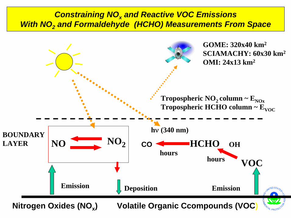
Constraining NOx and Reactive VOC EmissionsWith NO2 and Formaldehyde (HCHO) Measurements From Space

Emission

NOhν (420 nm)

O3, RO2

NO2

HNO3

1 day

Nitrogen Oxides (NOx) Volatile Organic Ccompounds (VOC)

Emission

VOC

OHHCHOhν (340 nm)

hourshours

COBOUNDARYLAYER

~ 2 km

Tropospheric NO2 column ~ ENOxTropospheric HCHO column ~ EVOC

Deposition

GOME: 320x40 km2

SCIAMACHY: 60x30 km2

OMI: 24x13 km2

http://www-as.harvard.edu/chemistry/trop/satellite/index.html

TOP-DOWN CONSTRAINTS ON NOx EMISSION INVENTORIESFROM OMI NO2 DATA INTERPRETED WITH GEOS-Chem

Tropospheric NO2 (March 2006)

OMIobservations

GEOS-Chemwith EPA 1999 emissions

OMI – GEOS-Chem differenceBoersma et al. [2007]

Fitting OMI NO2 with GEOS-Chem requires• 25% decrease in power plant emissions• 30% increase in vehicle emissionsrelative to EPA 1999 official inventory

Formaldehyde Columns From OMI (Jun-Aug 2006):high values are due to biogenic isoprene (main reactive VOC)

OMI GEOS-Chem model w/best prior (MEGAN) biogenic VOC emissions

MEGAN emission hot spots not substantiated by the OMI data

Millet et al. [2007]

Documents

8-hr Ozone National Ambient Air Quality Standard (NAAQS