Embed Size (px)
Citation preview

Network Analysis, Inc. 4151 W. Lindbergh Way, Chandler, AZ 85226
Phone 480-756-0512 Fax 480-820-1991 [email protected] www.sinda.com
SINDA/G for Patran MLI and Honeycomb Panel
Workshop 8
• Level: Intermediate • Software Requirement: SINDA/G for Patran • Objectives:
− MLI Simulation − Honeycomb Panel Simulation − Contact and Gap Radiation − Contact Visualizer − MLI in orbit

SINDA/G for Patran Workshop 8 September 2006
Copyright © 2006 by Network Analysis Inc. All rights reserved. No part of this publication may be reproduced, stored in a retrieval system, or transmitted, in any form or by any means, electronic, mechanical, photocopying, recording, or otherwise, without the prior written permission of the author and publisher.

SINDA/G for Patran Workshop 8 3
MLI and Honeycomb Panel
1. Brief Introduction of MLI Multi-Layer Insulation (MLI) is an insulation made of successive layers of separated low emissivity surfaces that is effective in high vacuum environments. Heat transfer through multilayer insulation is a combination of radiation, solid conduction and under atmospheric conditions, gaseous conduction. Because these heat-transfer mechanisms operate simultaneously and interact with each other, the thermal conductivity of an insulation is not strictly defined in terms of variables such as temperature, density, or physical properties of the component materials. It is therefore useful to refer to either an effective conductivity, K eff , or an effective emissivity, ε* (referred to as E-Star for the MLI blanket). Both of these values can be derived or adjusted experimentally from the data of thermal vacuum tests, or real missions in orbit. These definitions are from “Spacecraft Thermal Control Handbook” edited by David G. Gilmore , AIAA. 2. MLI Simulation methods (1) E-star (ε*) and Effective emissivity (ε eff ) This method uses the e-star (ε*) or effective emissivity (ε eff ) directly on the spacecraft wall.
The ε* is defined as effective emissivity from spacecraft wall to MLI outer surface. It is actually an experimental parameter which already includes both radiation and conduction factors. The ε* does not include the effect of the thermal property of MLI outer surface. That is to say, the effect of the thermal property of MLI outer surface is actually ignored. This can be a simple way to simulate the heat loss through MLI for an instrument or a part, whose temperature does not mainly depend on the local MLI blanket. Of course, ε eff can be used here instead of ε*.
The ε eff is defined as effective emissivity from the spacecraft wall, all the way through MLI, and to the space environment. That is to say, the effect of the thermal property of MLI outer surface is already taken into account. For the whole spacecraft thermal model, or a system level model, the ε eff should be used instead of ε*, because the thermal property of MLI outer surface has a significant effect on the overall thermal balance and temperature level. In these cases, ε* should not be used any longer.
The emissivity of coating on MLI outer surface ε out depends on the coating on this exposed surface, which provides a desired α/ε ratio.
4
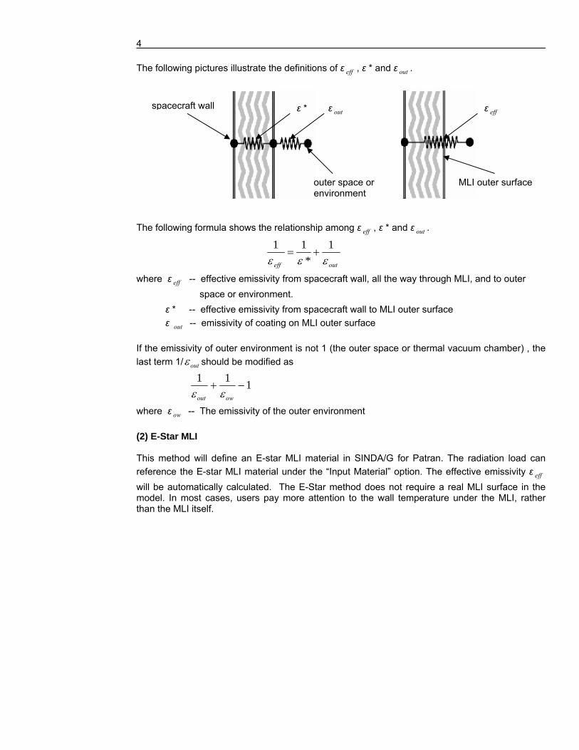
The following pictures illustrate the definitions of ε eff , ε * and ε out . The following formula shows the relationship among ε eff , ε * and ε out .
outeff εεε1
*11+=
where ε eff -- effective emissivity from spacecraft wall, all the way through MLI, and to outer space or environment.
ε * -- effective emissivity from spacecraft wall to MLI outer surface ε out -- emissivity of coating on MLI outer surface If the emissivity of outer environment is not 1 (the outer space or thermal vacuum chamber) , the last term 1/ outε should be modified as
111−+
owout εε
where ε ow -- The emissivity of the outer environment (2) E-Star MLI This method will define an E-star MLI material in SINDA/G for Patran. The radiation load can reference the E-star MLI material under the “Input Material” option. The effective emissivity ε eff will be automatically calculated. The E-Star method does not require a real MLI surface in the model. In most cases, users pay more attention to the wall temperature under the MLI, rather than the MLI itself.
spacecraft wall ε * ε out
outer space or environment
ε eff
MLI outer surface

SINDA/G for Patran Workshop 8 5
The variable definitions in E-star MLI material: External IR Emissivity: the emissivity of coating on MLI outer surface External UV Emissivity: the absorptivity of coating on MLI outer surface External IR Specularity: the specularity ratio of coating on MLI outer surface External UV Specularity: the specularity ratio of coating on MLI outer surface Overall E-Star: the effective emissivity from spacecraft wall to MLI outer surface When external radiation codes are used to calculate the view factors, SINDA/G translator will automatically generate arithmetic MLI nodes in the SINDA/G input file to represent MLI outer surface. You can find these synthetic arithmetic nodes in the .sin file. This happens only when the enclosures or primitive loads are used. The reason we add MLI nodes is that we may need to add orbital flux to these MLI nodes. Please note: these MLI nodes will be generated automatically as long as external radiation codes are involved, no matter if the orbital flux is needed or not. For ambient space or gap radiation loads, no external radiation codes are involved, therefore the translator will not generate MLI nodes. For enclosures and primitives loads, external radiation codes are involved and the translator will generate Arithmetic MLI nodes in SINDA/G input file. (3) Contact or Gap Radiation You can also create a real surface in the model to represent the MLI outer surface. In this case, the MLI nodes are also a part of the FEM model. The temperature result can be post-processed and shown as temperature contours. If you want to distinguish the temperature contours of MLI nodes and the spacecraft wall, the Patran group can store these MLI surfaces or spacecraft wall, so that you can display or hide the temperature contours for either the spacecraft wall or MLI blankets. Contact loads can be used to simulate the effective conductivity (K eff ) of MLI. The following
parameters can be used as references. For lower temperature cases, K eff varies from 3.0E-4 to
7.0E-4 W/m.C°. For higher temperature cases, K eff varies from 4.0E-3 to 9.0E-3 W/m.C°. The
contact coefficient h of the contact load can be calculated by the following formula:
dK
h eff=
where h -- the contact coefficient between spacecraft wall and MLI outer surface. K eff -- the effective conductivity of MLI blanket, an experimental parameter. d -- the overall average thickness of the MLI blanket. Gap radiation loads can be used to simulate ε* of MLI blanket. We need to input two emissivities for the gap radiation load. We can input ε * into either of them, input 1 into another data box. ε * varies from 0.01 to 0.03, Here in workshop 8, we use 0.02 for the ε* value.

6
It is the user’s decision to choose which method to use. In general, the effective conductivity is more accurate in lower temperature cases, the effective emissivity is more accurate in higher temperature cases. Again, these parameters are derived from experiments or real missions. The same concept should be used in thermal design, thermal vacuum tests and orbital remote measurement. For the Contact or Gap Radiation loads, the “projection method” is used to determine the contact area and links. The projection is always from the slave to the master. The meshes on the master and slave do not have to match each other. Although the matching meshes will certainly cause the most accurate result, it is not always convenient to keep the mesh congruent and lined up across the interface. There are two main reasons to determine which surface should be the master or slave: projection efficiency and result accuracy. Usually we will recommend using a similar mesh size on both the master and slave surfaces. We recommend the following guidelines:
1. Use the smaller surface as the slave for better projection efficiency. 2. Use the surface with the finer mesh as the slave for better result accuracy. 3. If the bigger surface has a much finer mesh, use it as the slave for better accuracy, even
though it may be a little bit slower. 4. Avoid using a very rough mesh for the slave, no matter whether the surface is bigger or
smaller. 3. Brief Introduction of Honeycomb Panel Honeycomb composites of various types are commonly used on spacecraft as equipment shelves, solar-array substrates, etc. Because of its construction, a honeycomb has directionally dependent conductivities. Some equations were developed to calculate the effective conductivity through honeycomb core material. These equations can be found in ”Spacecraft Thermal Control Handbook” edited by David G. Gilmore, AIAA. In many engineering projects, the experimental effective conductivity is used to simulate the heat transfer of honeycomb panel. Sometimes heat pipes, frames or small mechanical parts are buried into honeycomb panels. This will greatly increase the thermal conduction of honeycomb panel as a whole. In these cases, you probably need to calculate all the conductors individually and then combine them together. 4. Honeycomb Panel simulation methods (1) Simple Plate If the material of honeycomb core and face sheets is aluminum, and the gradient across the thickness can be ignored based on the accuracy requirements, the honeycomb panel can be
SINDA/G for Patran Workshop 8 7
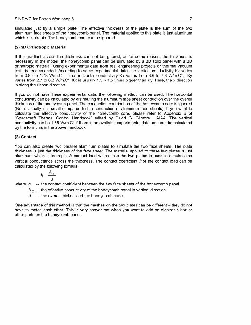
simulated just by a simple plate. The effective thickness of the plate is the sum of the two aluminum face sheets of the honeycomb panel. The material applied to this plate is just aluminum which is isotropic. The honeycomb core can be ignored. (2) 3D Orthotropic Material If the gradient across the thickness can not be ignored, or for some reason, the thickness is necessary in the model, the honeycomb panel can be simulated by a 3D solid panel with a 3D orthotropic material. Using experimental data from real engineering projects or thermal vacuum tests is recommended. According to some experimental data, the vertical conductivity Kz varies from 0.85 to 1.78 W/m.C°, The horizontal conductivity Kx varies from 3.6 to 7.3 W/m.C°, Ky varies from 2.7 to 6.2 W/m.C°, Kx is usually 1.3 ~ 1.5 times bigger than Ky. Here, the x direction is along the ribbon direction. If you do not have these experimental data, the following method can be used. The horizontal conductivity can be calculated by distributing the aluminum face sheet conduction over the overall thickness of the honeycomb panel. The conduction contribution of the honeycomb core is ignored (Note: Usually it is small compared to the conduction of aluminum face sheets). If you want to calculate the effective conductivity of the honeycomb core, please refer to Appendix B of “Spacecraft Thermal Control Handbook” edited by David G. Gilmore , AIAA. The vertical conductivity can be 1.55 W/m.C° if there is no available experimental data, or it can be calculated by the formulas in the above handbook. (3) Contact You can also create two parallel aluminum plates to simulate the two face sheets. The plate thickness is just the thickness of the face sheet. The material applied to these two plates is just aluminum which is isotropic. A contact load which links the two plates is used to simulate the vertical conductance across the thickness. The contact coefficient h of the contact load can be calculated by the following formula:
dKh Z=
where h -- the contact coefficient between the two face sheets of the honeycomb panel. K Z -- the effective conductivity of the honeycomb panel in vertical direction. d -- the overall thickness of the honeycomb panel. One advantage of this method is that the meshes on the two plates can be different – they do not have to match each other. This is very convenient when you want to add an electronic box or other parts on the honeycomb panel.
8
Problem 1
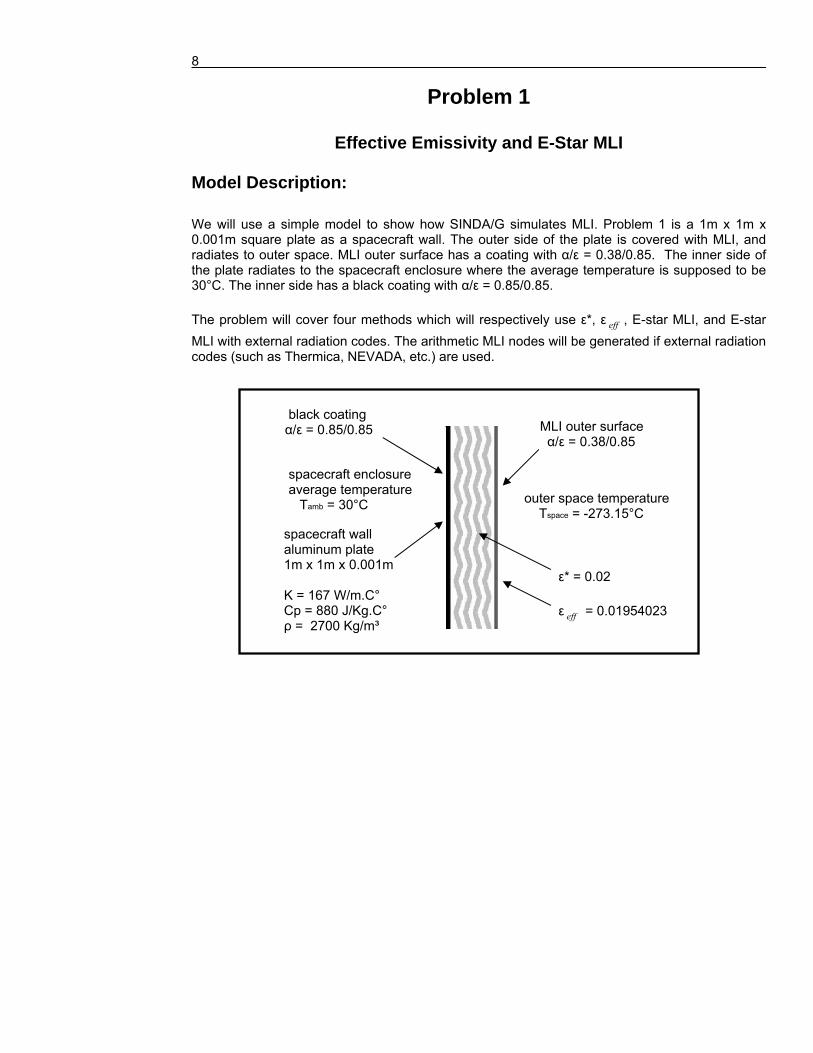
Effective Emissivity and E-Star MLI Model Description: We will use a simple model to show how SINDA/G simulates MLI. Problem 1 is a 1m x 1m x 0.001m square plate as a spacecraft wall. The outer side of the plate is covered with MLI, and radiates to outer space. MLI outer surface has a coating with α/ε = 0.38/0.85. The inner side of the plate radiates to the spacecraft enclosure where the average temperature is supposed to be 30°C. The inner side has a black coating with α/ε = 0.85/0.85. The problem will cover four methods which will respectively use ε*, ε eff , E-star MLI, and E-star MLI with external radiation codes. The arithmetic MLI nodes will be generated if external radiation codes (such as Thermica, NEVADA, etc.) are used.
spacecraft wall aluminum plate 1m x 1m x 0.001m K = 167 W/m.C° Cp = 880 J/Kg.C° ρ = 2700 Kg/m³
black coating α/ε = 0.85/0.85
spacecraft enclosure average temperature Tamb = 30°C
MLI outer surface α/ε = 0.38/0.85
outer space temperature Tspace = -273.15°C
ε* = 0.02 ε eff = 0.01954023

SINDA/G for Patran Workshop 8 9
Suggested Exercise Steps:
• Create a new database and name it mli_plate1.db
• Create a 1 x 1 rectangular surface
• Mesh the surface with one Quad element
• Specify an Isotropic Material and an E-Star MLI material
• Define a 2D Shell Property
• Apply an Ambient Space load on the spacecraft wall
• Apply an Ambient Space load on MLI outer surface
• Perform the Analysis
• Import the .nrf result file back into Patran
• Display the Result
• Examine Input and Result files
• Modify the Ambient Space load on MLI outer surface
• Analysis, Access Result and Display
• Examine Input and Result files
• Modify the Ambient Space load on MLI outer surface
• Analysis, Access Result and Display
• Examine Input and Result files
• Delete the Ambient Space load on the MLI outer surface
• Apply an Enclosures load on the MLI outer surface
• Perform the Analysis
• Access Result , Display and Examine files

10
Exercise Procedure: 1. Create a new database and name it mli_plate1.db File/New…
File name: mli_plate1.db
OK
Tolerance: Based on Model
Analysis Code: SINDA/G
Analysis Type: Thermal OK
2. Create a 1 x 1 rectangular surface
Geometry
Action: Create
Object: Surface
Method: XYZ
Vector Coordinates List: <1 1 0>
Origin Coordinates List: [0 0 0]
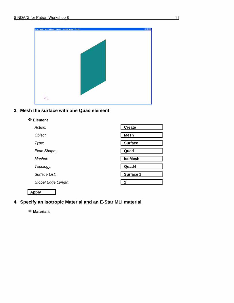
Apply Click on the Iso 2 View icon to obtain a 3D view of the rectangular surface. Iso 2 View Click on the Fit View icon and Smooth Shaded icon Fit View Smooth Shade Your model should look like the following figure:
SINDA/G for Patran Workshop 8 11
3. Mesh the surface with one Quad element
Element
Action: Create
Object: Mesh
Type: Surface
Elem Shape: Quad
Mesher: IsoMesh
Topology: Quad4
Surface List: Surface 1
Global Edge Length: 1 Apply
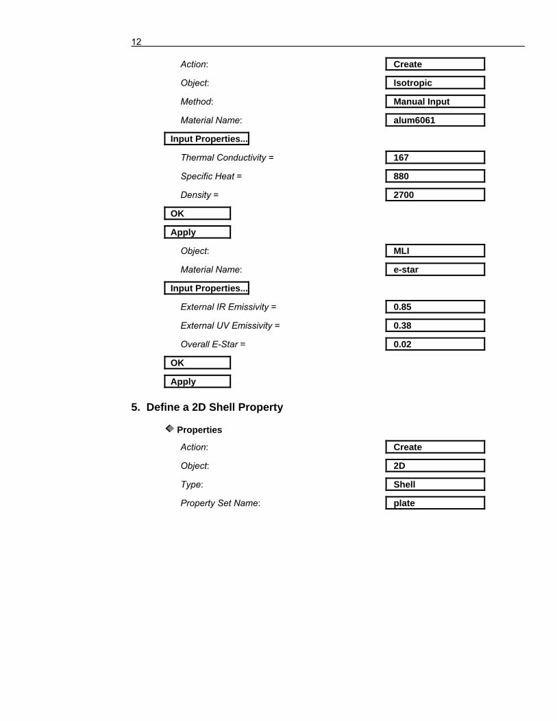
4. Specify an Isotropic Material and an E-Star MLI material
Materials
12
Action: Create
Object: Isotropic
Method: Manual Input
Material Name: alum6061
Input Properties...
Thermal Conductivity = 167
Specific Heat = 880
Density = 2700
OK
Apply
Object: MLI
Material Name: e-star
Input Properties...
External IR Emissivity = 0.85
External UV Emissivity = 0.38
Overall E-Star = 0.02
OK
Apply 5. Define a 2D Shell Property
Properties
Action: Create
Object: 2D
Type: Shell
Property Set Name: plate

SINDA/G for Patran Workshop 8 13
Input Properties...
Material Name: m:alum6061
Thickness: 0.001
OK Verify the Surface or Face icon is checked. Surface or Face
Select Members: Surface 1
Add
Apply 6. Apply an Ambient Space load on the spacecraft wall
Load/BCs
Action: Create
Object: Radiation(SINDA/G)
Type: Element Uniform
Option: Ambient Space
New Set Name: inner_rad
Target Element Type: 2D
Input Data...
Surface Option: Bottom
Bottom Surf Emissivity: 0.85
View Factor: 1
Ambient Temperature Switch: Temperature
Ambient Temperature: 30
OK

14
Select Application Region...
Geometry Filter: Geometry Verify the Surface or Face icon is checked. Surface or Face
Select Surfaces or Edges: Surface 1
Add
OK
Apply 7. Apply an Ambient Space load on MLI outer surface
Load/BCs
Action: Create
Object: Radiation(SINDA/G)
Type: Element Uniform
Option: Ambient Space
New Set Name: outer_rad
Target Element Type: 2D
Input Data...
Surface Option: Top
Top Surf Emissivity: 0.02
View Factor: 1
Ambient Temperature Switch: Temperature
Ambient Temperature: -273.15
OK

SINDA/G for Patran Workshop 8 15
Select Application Region...
Select Surfaces or Edges: Surface 1
Add
OK
Apply Your model should look like the following figure: 8. Perform the Analysis
Analysis
Action: Analyze
Object: Entire Model
Method: Translate and Run
Job Name: mli_plate1
Apply
16
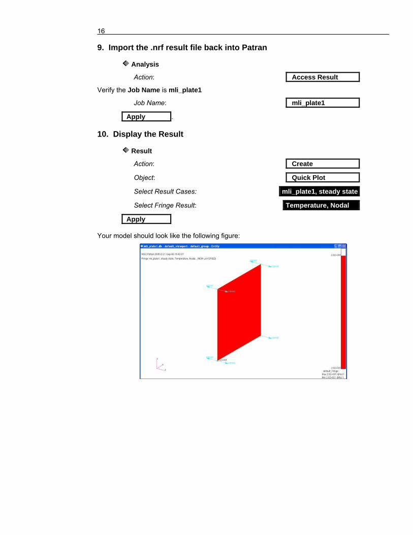
9. Import the .nrf result file back into Patran
Analysis
Action: Access Result
Verify the Job Name is mli_plate1
Job Name: mli_plate1
Apply . 10. Display the Result
Result
Action: Create
Object: Quick Plot
Select Result Cases: mli_plate1, steady state
Select Fringe Result: Temperature, Nodal
Apply Your model should look like the following figure:
SINDA/G for Patran Workshop 8 17
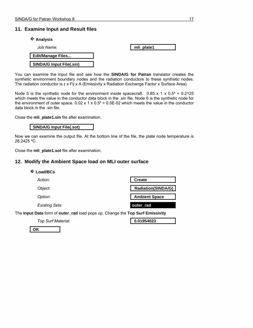
11. Examine Input and Result files
Analysis
Job Name: mli_plate1
Edit/Manage Files...
SINDA/G Input File(.sin) You can examine the input file and see how the SINDA/G for Patran translator creates the synthetic environment boundary nodes and the radiation conductors to these synthetic nodes. The radiation conductor is ε x Fij x A (Emissivity x Radiation Exchange Factor x Surface Area). Node 5 is the synthetic node for the environment inside spacecraft. 0.85 x 1 x 0.5² = 0.2125 which meets the value in the conductor data block in the .sin file. Node 6 is the synthetic node for the environment of outer space. 0.02 x 1 x 0.5² = 0.5E-02 which meets the value in the conductor data block in the .sin file. Close the mli_plate1.sin file after examination.
SINDA/G Input File(.sot)
Now we can examine the output file. At the bottom line of the file, the plate node temperature is 28.2425 ºC. Close the mli_plate1.sot file after examination. 12. Modify the Ambient Space load on MLI outer surface
Load/BCs
Action: Create
Object: Radiation(SINDA/G)
Option: Ambient Space
Existing Sets: outer_rad
The Input Data form of outer_rad load pops up. Change the Top Surf Emissivity
Top Surf Material: 0.01954023
OK
18
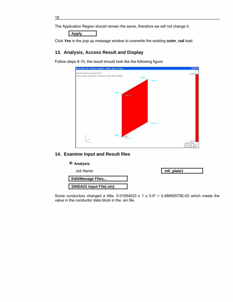
The Application Region should remain the same, therefore we will not change it.
Apply
Click Yes in the pop up message window to overwrite the existing outer_rad load.
13. Analysis, Access Result and Display Follow steps 8-10, the result should look like the following figure: 14. Examine Input and Result files
Analysis
Job Name: mli_plate1
Edit/Manage Files...
SINDA/G Input File(.sin) Some conductors changed a little. 0.01954023 x 1 x 0.5² = 0.48850575E-02 which meets the value in the conductor data block in the .sin file.

SINDA/G for Patran Workshop 8 19
Close the mli_plate1.sin file after examination.
SINDA/G Input File(.sot)
Now the plate node temperature is 28.2824 ºC. The temperature is a little bit higher than the forst result when the E-star = 0.02 is used, because the emissivity of MLI outer surface is considered. Close the mli_plate1.sot file after examination. 15. Modify the Ambient Space load on MLI outer surface
Load/BCs
Action: Create
Object: Radiation(SINDA/G)
Option: Ambient Space
Existing Sets: outer_rad
The Input Data form of outer_rad load pops up. Change the form type.
Surface Option: Top
Form Type: Input Material
Click the e-star material in the Coating or MLI Material List window.
Top Surf Material: m:e-star
View Factor: 1
Ambient Temperature Switch: Temperature
Ambient Temperature: -273.15
OK
The Application Region should remain the same, therefore we will not change it.
Apply
Click Yes in the pop up message window to overwrite the existing outer_rad load.
16. Analysis, Access Result and Display Follow steps 8-10, the result should look like the following figure:

20
17. Examine Input and Result files
Analysis
Job Name: mli_plate1
Edit/Manage Files...
SINDA/G Input File(.sin) You will find the .sin file is the same as before. The SINDA/G Translator automatically calculates the ε eff .
Close the mli_plate1.sin file after examination.
SINDA/G Input File(.sot)
The plate node temperature is also the same as before. Close the mli_plate1.sot file after examination. 18. Delete the Ambient Space load on MLI outer surface
Load/BCs

SINDA/G for Patran Workshop 8 21
Action: Delete
Object: Radiation(SINDA/G)
Option: Ambient Space
Existing Sets: outer_rad
Apply 19. Apply an Enclosures load on MLI outer surface
Load/BCs
Action: Create
Object: Radiation(SINDA/G)
Type: Element Uniform
Option: Enclosures
New Set Name: outer_rad_sf
Target Element Type: 2D
Input Data...
Surface Option: Top
Form Type: Input Material
Clicking the e-star material in the Coating or MLI Material List window.
Top Surf Material: m:e-star
Enclosure ID: 1
Small Facets Method
OK
Select Application Region... Verify the Surface or Face icon is checked. Surface or Face
22
Select Surfaces or Edges: Surface 1
Add
OK
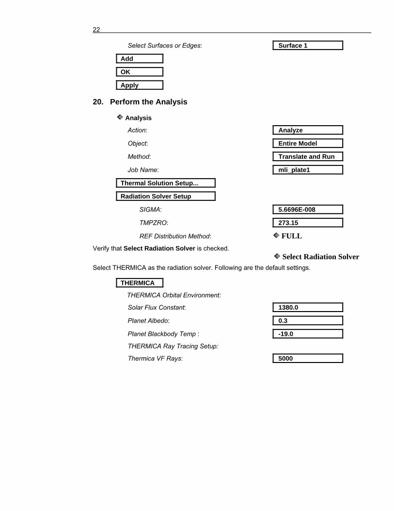
Apply 20. Perform the Analysis
Analysis
Action: Analyze
Object: Entire Model
Method: Translate and Run
Job Name: mli_plate1
Thermal Solution Setup...
Radiation Solver Setup
SIGMA: 5.6696E-008
TMPZRO: 273.15
REF Distribution Method: FULL
Verify that Select Radiation Solver is checked. Select Radiation Solver
Select THERMICA as the radiation solver. Following are the default settings.
THERMICA
THERMICA Orbital Environment:
Solar Flux Constant: 1380.0
Planet Albedo: 0.3
Planet Blackbody Temp : -19.0
THERMICA Ray Tracing Setup:
Thermica VF Rays: 5000

SINDA/G for Patran Workshop 8 23
Thermica Flux Rays: 5000
Confidence Level(%): 99.000
OK The THERMICA button is marked “default” to show that it is the current default radiation solver.
OK
SINDA/G Option: Single Precision (Fortran)
OK
Apply Unless it is your first time running THERMICA, a caution window will pop up to ask if you want to overwrite the existing THERMICA configuration file, click OK to overwrite. The THERMICA window will pop up.
Import Data There are three methods to import a model into THERMICA: Graphic editor, Modeler or Ascii. Modeler and Ascii are most commonly used. Here we use the Modeler method.
Modeler
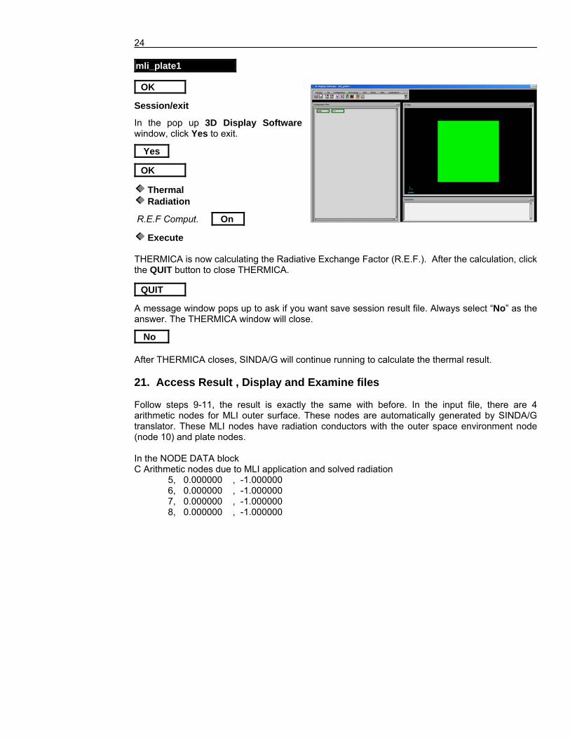
24
mli_plate1
OK
Session/exit
In the pop up 3D Display Software window, click Yes to exit.
Yes
OK
Thermal Radiation
R.E.F Comput. On
Execute THERMICA is now calculating the Radiative Exchange Factor (R.E.F.). After the calculation, click the QUIT button to close THERMICA.
QUIT
A message window pops up to ask if you want save session result file. Always select “No” as the answer. The THERMICA window will close.
No After THERMICA closes, SINDA/G will continue running to calculate the thermal result. 21. Access Result , Display and Examine files Follow steps 9-11, the result is exactly the same with before. In the input file, there are 4 arithmetic nodes for MLI outer surface. These nodes are automatically generated by SINDA/G translator. These MLI nodes have radiation conductors with the outer space environment node (node 10) and plate nodes. In the NODE DATA block C Arithmetic nodes due to MLI application and solved radiation 5, 0.000000 , -1.000000 6, 0.000000 , -1.000000 7, 0.000000 , -1.000000 8, 0.000000 , -1.000000

SINDA/G for Patran Workshop 8 25
In the CONDUCTOR DATA block C Conductors due to MLI node to surface links -11, 1, 5, 0.5000000E-02 -12, 2, 6, 0.5000000E-02 -13, 3, 7, 0.5000000E-02 -14, 4, 8, 0.5000000E-02 C Conductors due to solved radiation loads -15, 5, 10, 0.2125000 -16, 6, 10, 0.2125000 -17, 7, 10, 0.2125000 -18, 8, 10, 0.2125000 In the output file. At the bottom line of the file, the plate node temperature is still 28.2425 ºC. the MLI node temperature is -155.7772 ºC. **** OUTPUT TEMPERATURES IN DEGREES **** T 1 = 28.2824 T 2 = 28.2824 T 3 = 28.2824 T 4 = 28.2824 T 5 = -155.7772 T 6 = -155.7772 T 7 = -155.7772 T 8 = -155.7772 T 9 = 30.0000 T 10 = -273.1500 To complete this exercise, close the database and quit Patran. File/Quit...
26
Problem 2
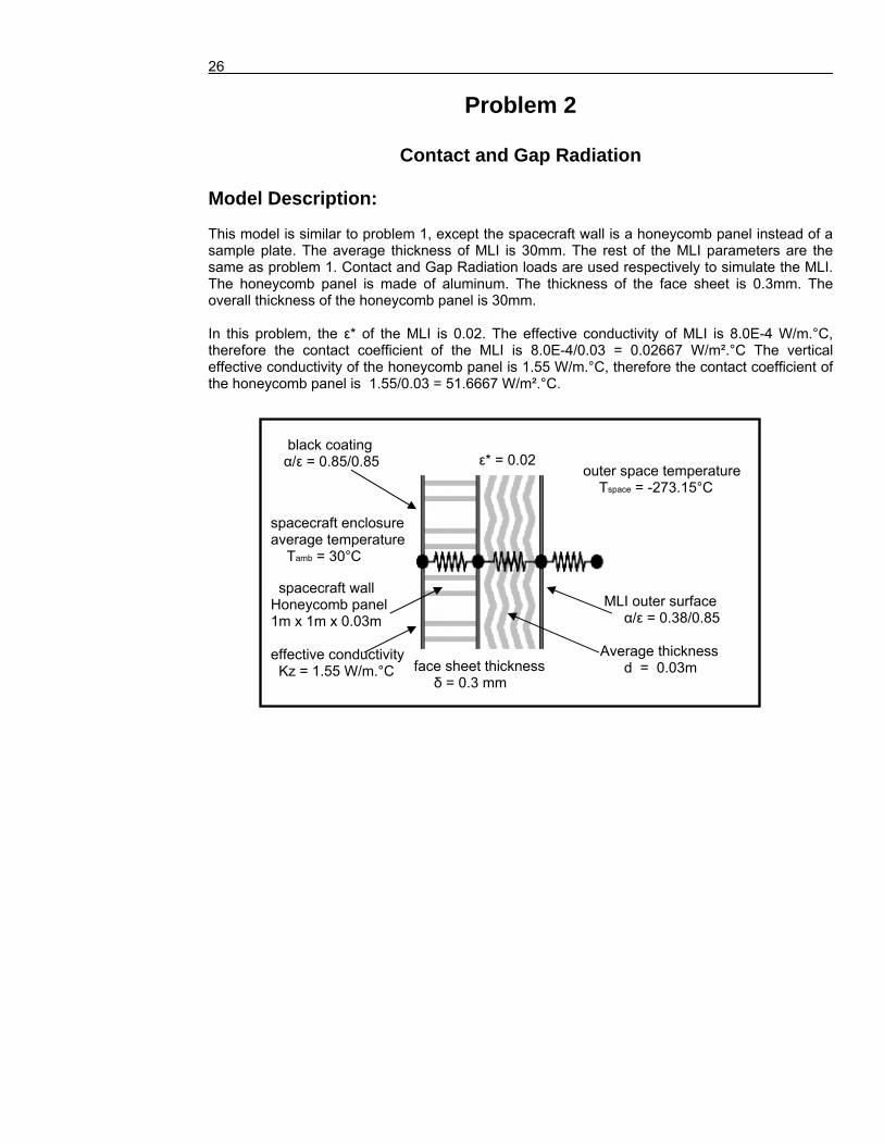
Contact and Gap Radiation Model Description: This model is similar to problem 1, except the spacecraft wall is a honeycomb panel instead of a sample plate. The average thickness of MLI is 30mm. The rest of the MLI parameters are the same as problem 1. Contact and Gap Radiation loads are used respectively to simulate the MLI. The honeycomb panel is made of aluminum. The thickness of the face sheet is 0.3mm. The overall thickness of the honeycomb panel is 30mm. In this problem, the ε* of the MLI is 0.02. The effective conductivity of MLI is 8.0E-4 W/m.°C, therefore the contact coefficient of the MLI is 8.0E-4/0.03 = 0.02667 W/m².°C The vertical effective conductivity of the honeycomb panel is 1.55 W/m.°C, therefore the contact coefficient of the honeycomb panel is 1.55/0.03 = 51.6667 W/m².°C.
spacecraft wall Honeycomb panel 1m x 1m x 0.03m effective conductivity Kz = 1.55 W/m.°C
black coating α/ε = 0.85/0.85
spacecraft enclosure average temperature Tamb = 30°C
MLI outer surface α/ε = 0.38/0.85 Average thickness d = 0.03m
outer space temperature Tspace = -273.15°C
ε* = 0.02
face sheet thickness δ = 0.3 mm

SINDA/G for Patran Workshop 8 27
Suggested Exercise Steps:
• Create a new database and name it mli_honeycomb.db
• Create three 1 x 1 rectangular surfaces
• Mesh the three surfaces
• Specify an Isotropic Material • Define 2D Shell Properties
• Apply two Ambient Space loads
• Apply a Gap Radiation to simulate MLI
• Apply a Contact to simulate the honeycomb panel
• Perform the Analysis
• Import the .nrf result file back into Patran
• Display the Result
• Examine the nodal temperature result
• Dsiaply the contact visualizer
• Delete the gap radiation load
• Apply a Contact to simulate the MLI
• Analysis, Access Result and Display

28
Exercise Procedure:
1. Create a new database and name it mli_honeycomb.db File/New…
File name: mli_honeycomb.db
OK
Tolerance: Based on Model
Analysis Code: SINDA/G
Analysis Type: Thermal OK
2. Create three 1 x 1 rectangular surfaces
Geometry
Action: Create
Object: Surface
Method: XYZ
Vector Coordinates List: <1 1 0>
Origin Coordinates List: [0 0 0]
Apply Click on the Iso 2 View icon to obtain a 3D view of the rectangular surface. Iso 2 View Click on the Fit View icon and Smooth Shaded icon Fit View Smooth Shaded

SINDA/G for Patran Workshop 8 29
We deliberately enlarge the distance 10 times between the three surfaces for a better view. The enlarged distance will not affect the thermal result of this model, because contact and gap radiation do not actually use the distance in the calculations.
Origin Coordinates List: [0 0 0.3]
Apply
Origin Coordinates List: [0 0 0.6]
Apply Your model should look like the following figure: 3. Mesh the surface with one Quad element
Element
Action: Create
Object: Mesh
Type: Surface
Elem Shape: Quad
Mesher: IsoMesh

30
Topology: Quad4
Click in the Surface List data box, pick surface 3 in the far right, hold the shift key and pick surface 2 at the middle.
Surface List: Surface 3 2
Global Edge Length: 0.2 Apply
Contact and Gap Radiation do not require the two meshes match each other. Let’s mesh the surface 1 with Tria elements and Global Edge Length = 0.1. You can mesh the three surfaces together with quad elements if you wish. We meshed surface 1 with Tria elements on purpose to show SINDA/G for Patran’s ability to automatically hook the mis-matched meshes.)
Elem Shape: Tria
Surface List: Surface 1
Global Edge Length: 0.1 Apply
Your model should look like the following figure:
SINDA/G for Patran Workshop 8 31
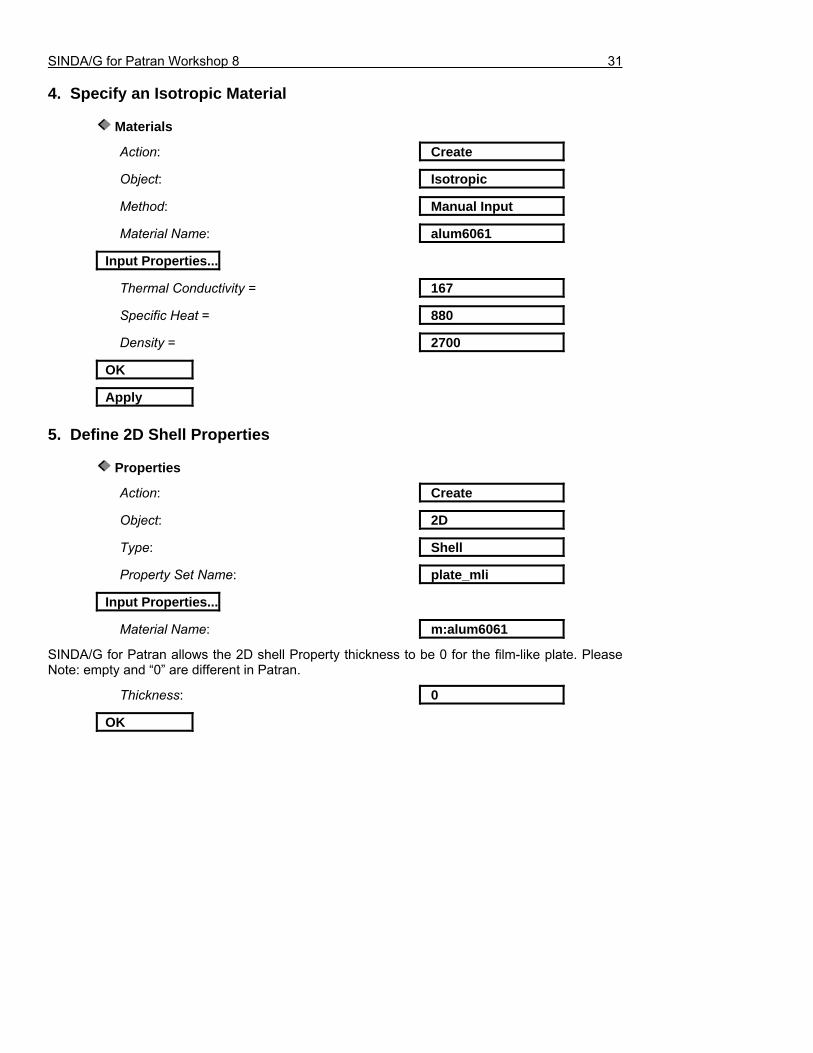
4. Specify an Isotropic Material
Materials
Action: Create
Object: Isotropic
Method: Manual Input
Material Name: alum6061
Input Properties...
Thermal Conductivity = 167
Specific Heat = 880
Density = 2700
OK
Apply 5. Define 2D Shell Properties
Properties
Action: Create
Object: 2D
Type: Shell
Property Set Name: plate_mli
Input Properties...
Material Name: m:alum6061
SINDA/G for Patran allows the 2D shell Property thickness to be 0 for the film-like plate. Please Note: empty and “0” are different in Patran.
Thickness: 0
OK
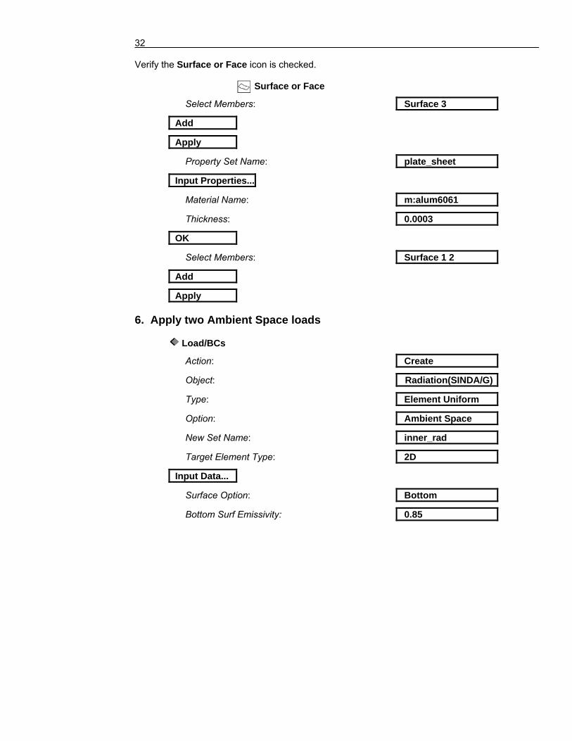
32
Verify the Surface or Face icon is checked. Surface or Face
Select Members: Surface 3
Add
Apply
Property Set Name: plate_sheet
Input Properties...
Material Name: m:alum6061
Thickness: 0.0003
OK
Select Members: Surface 1 2
Add
Apply 6. Apply two Ambient Space loads
Load/BCs
Action: Create
Object: Radiation(SINDA/G)
Type: Element Uniform
Option: Ambient Space
New Set Name: inner_rad
Target Element Type: 2D
Input Data...
Surface Option: Bottom
Bottom Surf Emissivity: 0.85

SINDA/G for Patran Workshop 8 33
View Factor: 1
Ambient Temperature Switch: Temperature
Ambient Temperature: 30
OK
Select Application Region...
Geometry Filter: Geometry Verify the Surface or Face icon is checked. Surface or Face
Select Surfaces or Edges: Surface 1
Add
OK
Apply
New Set Name: outer_rad
Target Element Type: 2D
Input Data...
Surface Option: Top
Top Surf Emissivity: 0.85
View Factor: 1
Ambient Temperature Switch: Temperature
Ambient Temperature: -273.15
OK
Select Application Region...
Select Surfaces or Edges: Surface 3
Add

34
OK
Apply 7. Apply a Gap Radiation to simulate MLI
Load/BCs
Action: Create
Object: Radiation(SINDA/G)
Type: Element Uniform
Option: Gap Radiation
New Set Name: gap_rad
Target Element Type: 2D
Region 2: 2D
Input Data...
Surface Option: Top
Top Surf Emissivity: 0.02
Since ε* = 0.02 already includes the all the radiation effects inside the MLI, the Emissivity 2 is set to 1 to keep the overall ε* = 0.02.
Emissivity 2: 1
OK
Select Application Region...
Geometry Filter: Geometry Check the upper Active List to activate the Application Region input.
Application region/Active List: Active List Check the Surface or Face icon on the pop up icon bar. Surface or Face
SINDA/G for Patran Workshop 8 35
Select Surfaces or Edges: Surface 2
Add
Check on the lower Active List to activate the Companion Region input.
Companion region/Active List: Active List
Select Surfaces or Edges: Surface 3
Add
OK
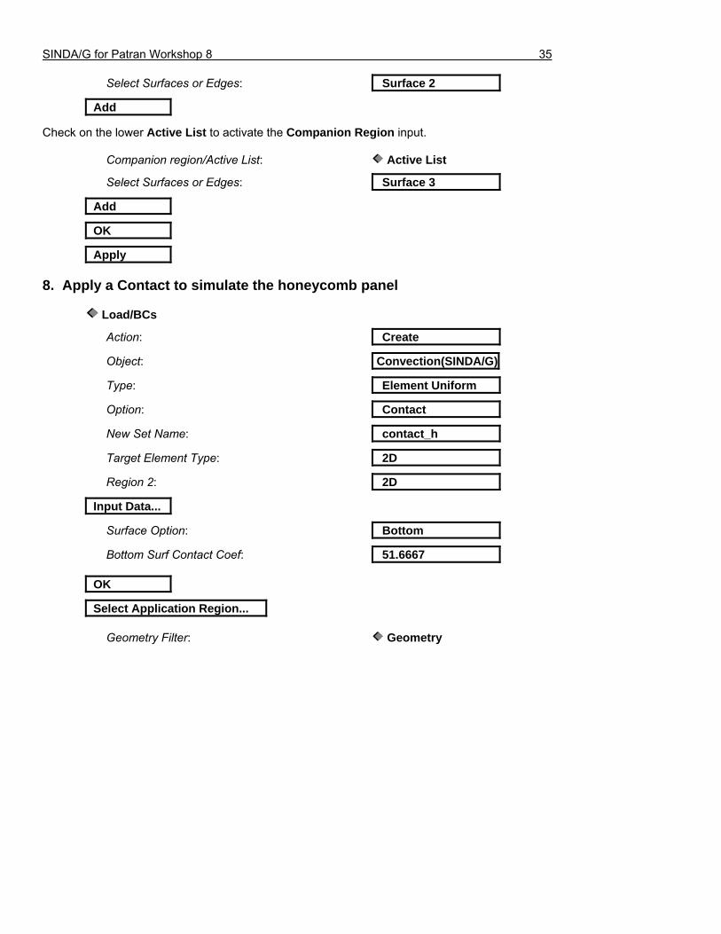
Apply 8. Apply a Contact to simulate the honeycomb panel
Load/BCs
Action: Create
Object: Convection(SINDA/G)
Type: Element Uniform
Option: Contact
New Set Name: contact_h
Target Element Type: 2D
Region 2: 2D
Input Data...
Surface Option: Bottom
Bottom Surf Contact Coef: 51.6667
OK
Select Application Region...
Geometry Filter: Geometry
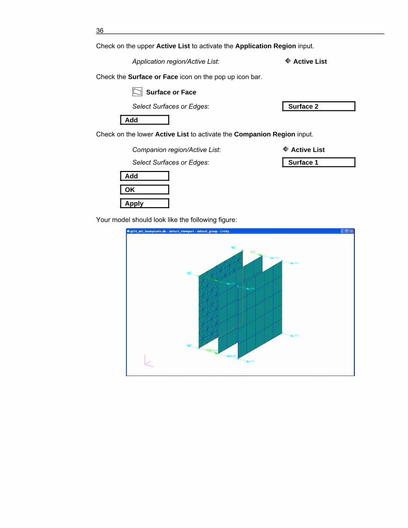
36
Check on the upper Active List to activate the Application Region input.
Application region/Active List: Active List Check the Surface or Face icon on the pop up icon bar. Surface or Face
Select Surfaces or Edges: Surface 2
Add
Check on the lower Active List to activate the Companion Region input.
Companion region/Active List: Active List
Select Surfaces or Edges: Surface 1
Add
OK
Apply Your model should look like the following figure:

SINDA/G for Patran Workshop 8 37
9. Perform the Analysis
Analysis
Action: Analyze
Object: Entire Model
Method: Translate and Run
Job Name: mli_honeycomb
Thermal Solution Setup...
Steady State Setup(SNSOR)
Choose Solution Routine: SNSOR
OK
SINDA/G Option: Single Precision (Fortran)
OK
Apply 10. Import the .nrf result file back into Patran
Analysis
Action: Access Result
Verify the Job Name is mli_honeycomb
Job Name: mli_honeycomb
Apply . 11. Display the Result
Result
Action: Create
Object: Quick Plot
Select Result Cases: mli_honeycomb, steady state
38
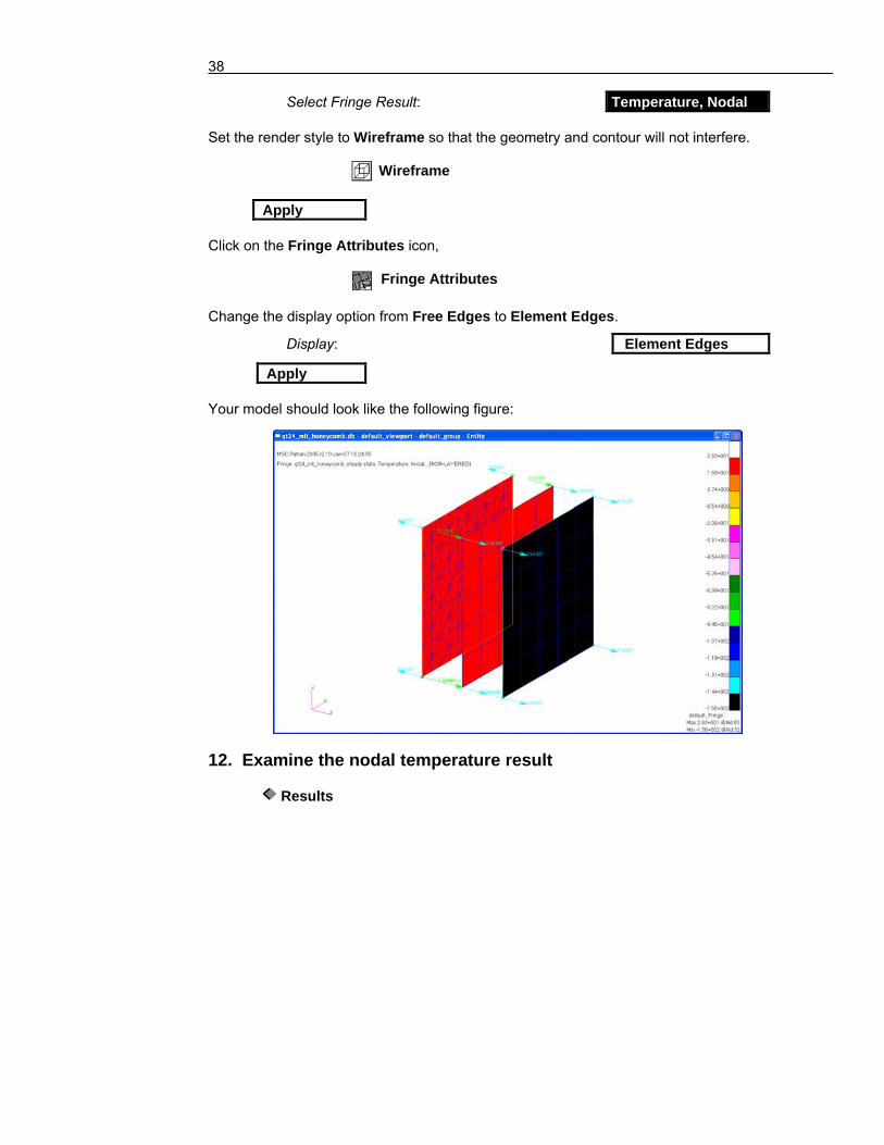
Select Fringe Result: Temperature, Nodal Set the render style to Wireframe so that the geometry and contour will not interfere.
Wireframe
Apply Click on the Fringe Attributes icon, Fringe Attributes Change the display option from Free Edges to Element Edges.
Display: Element Edges
Apply Your model should look like the following figure: 12. Examine the nodal temperature result
Results
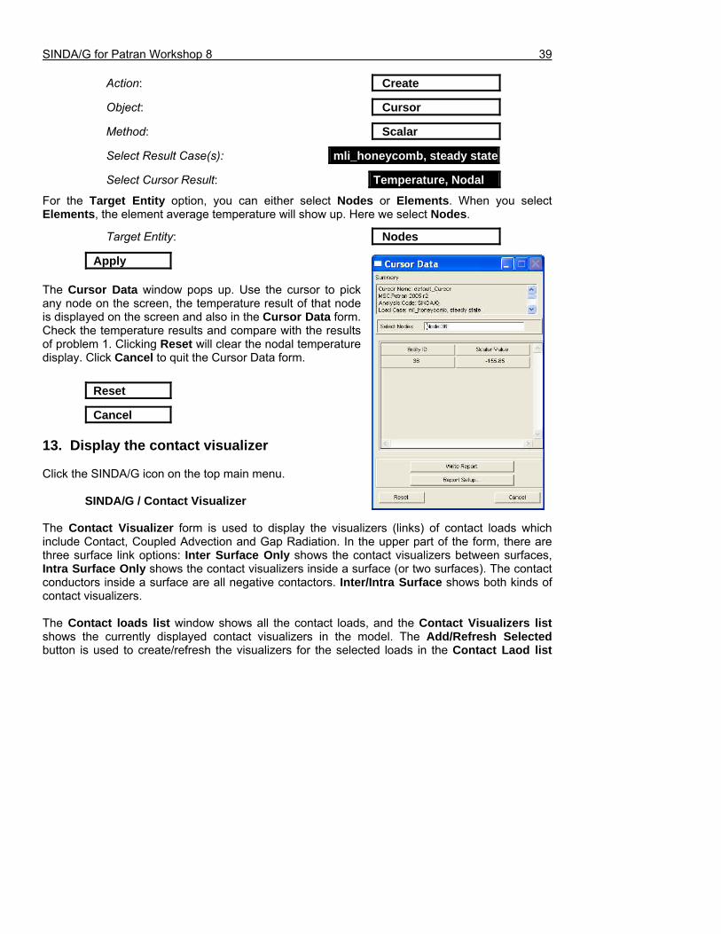
SINDA/G for Patran Workshop 8 39
Action: Create
Object: Cursor
Method: Scalar
Select Result Case(s): mli_honeycomb, steady state
Select Cursor Result: Temperature, Nodal
For the Target Entity option, you can either select Nodes or Elements. When you select Elements, the element average temperature will show up. Here we select Nodes.
Target Entity: Nodes
Apply The Cursor Data window pops up. Use the cursor to pick any node on the screen, the temperature result of that node is displayed on the screen and also in the Cursor Data form. Check the temperature results and compare with the results of problem 1. Clicking Reset will clear the nodal temperature display. Click Cancel to quit the Cursor Data form.
Reset
Cancel 13. Display the contact visualizer Click the SINDA/G icon on the top main menu. SINDA/G / Contact Visualizer The Contact Visualizer form is used to display the visualizers (links) of contact loads which include Contact, Coupled Advection and Gap Radiation. In the upper part of the form, there are three surface link options: Inter Surface Only shows the contact visualizers between surfaces, Intra Surface Only shows the contact visualizers inside a surface (or two surfaces). The contact conductors inside a surface are all negative contactors. Inter/Intra Surface shows both kinds of contact visualizers. The Contact loads list window shows all the contact loads, and the Contact Visualizers list shows the currently displayed contact visualizers in the model. The Add/Refresh Selected button is used to create/refresh the visualizers for the selected loads in the Contact Laod list

40
window. The Add/Refresh All button is used to add links for all loads together if there are no visualizers in the Contact Visualizers list window, or to refresh (update) the current contact visualizers in the model. The Remove Visualizers button is used to delete the selected contact visualizers in the Contact Visualizers list window.
Inter Surface Only
Add/Refresh All _
Rotate the model to view the contact visualizers. Try different operations to add/remove/refresh the two contact visualizers, Your model should look like the following figure:
Select all the contact visualizers in the Contact Visualizers list window, click the Remove Visualizers button.
Contact Visualizer list: gap_rad__visualizer
SINDA/G for Patran Workshop 8 41
contact_h__visualizer
Remove Visualizers_
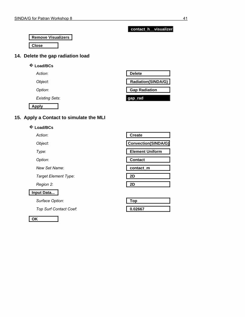
Close 14. Delete the gap radiation load
Load/BCs
Action: Delete
Object: Radiation(SINDA/G)
Option: Gap Radiation
Existing Sets: gap_rad
Apply 15. Apply a Contact to simulate the MLI
Load/BCs
Action: Create
Object: Convection(SINDA/G)
Type: Element Uniform
Option: Contact
New Set Name: contact_m
Target Element Type: 2D
Region 2: 2D
Input Data...
Surface Option: Top
Top Surf Contact Coef: 0.02667
OK
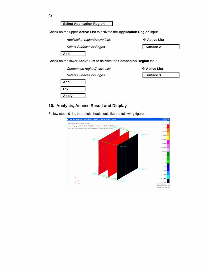
42
Select Application Region... Check on the upper Active List to activate the Application Region input
Application region/Active List: Active List
Select Surfaces or Edges: Surface 2
Add
Check on the lower Active List to activate the Companion Region input.
Companion region/Active List: Active List
Select Surfaces or Edges: Surface 3
Add
OK
Apply 16. Analysis, Access Result and Display Follow steps 9-11, the result should look like the following figure:
SINDA/G for Patran Workshop 8 43
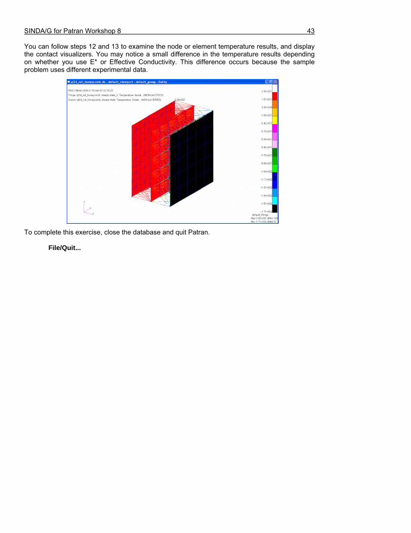
You can follow steps 12 and 13 to examine the node or element temperature results, and display the contact visualizers. You may notice a small difference in the temperature results depending on whether you use E* or Effective Conductivity. This difference occurs because the sample problem uses different experimental data. To complete this exercise, close the database and quit Patran. File/Quit...
44
Problem 3
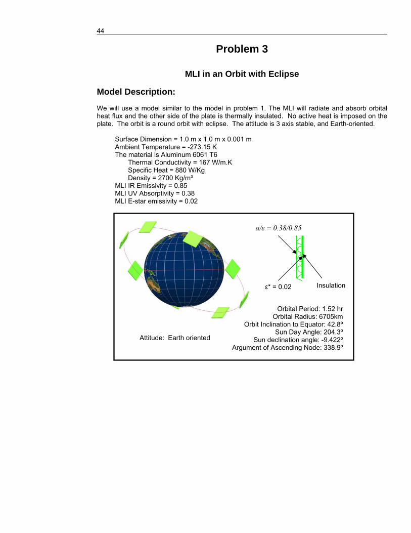
MLI in an Orbit with Eclipse Model Description: We will use a model similar to the model in problem 1. The MLI will radiate and absorb orbital heat flux and the other side of the plate is thermally insulated. No active heat is imposed on the plate. The orbit is a round orbit with eclipse. The attitude is 3 axis stable, and Earth-oriented.
Surface Dimension = 1.0 m x 1.0 m x 0.001 m Ambient Temperature = -273.15 K The material is Aluminum 6061 T6 Thermal Conductivity = 167 W/m.K Specific Heat = 880 W/Kg Density = 2700 Kg/m³ MLI IR Emissivity = 0.85 MLI UV Absorptivity = 0.38 MLI E-star emissivity = 0.02
Orbital Period: 1.52 hr Orbital Radius: 6705km
Orbit Inclination to Equator: 42.8º Sun Day Angle: 204.3º
Sun declination angle: -9.422º Argument of Ascending Node: 338.9º
Attitude: Earth oriented
0.38/0.85α/ε =
Insulationε* = 0.02

SINDA/G for Patran Workshop 8 45
Suggested Exercise Steps:
• Create a new database and name it mli_orbit.db
• Create a 1 x 1 rectangular surface
• Mesh the surface, Create Materials and Property
• Apply a Radiation/Enclosure load
• Perform the Analysis
• Access Result and Display
• Plot temperature curves in Thermal Studio
• Close Thermal Studio and quit Patran database
46
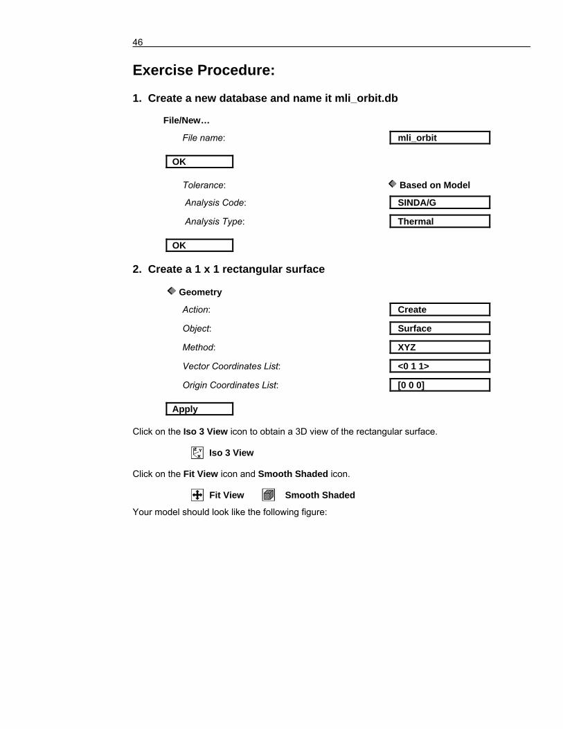
Exercise Procedure: 1. Create a new database and name it mli_orbit.db File/New…
File name: mli_orbit
OK
Tolerance: Based on Model
Analysis Code: SINDA/G
Analysis Type: Thermal OK
2. Create a 1 x 1 rectangular surface
Geometry
Action: Create
Object: Surface
Method: XYZ
Vector Coordinates List: <0 1 1>
Origin Coordinates List: [0 0 0] Apply
Click on the Iso 3 View icon to obtain a 3D view of the rectangular surface. Iso 3 View Click on the Fit View icon and Smooth Shaded icon. Fit View Smooth Shaded
Your model should look like the following figure:

SINDA/G for Patran Workshop 8 47
The surface orientation is deliberately designed to fit NEVADA’s orbital coordinate system. When yaw, pitch, and roll are all input as 0.000 in NEVADA’s orbital maneuvers form, the model coordinate system is equal to NEVADA’s orbital coordinate system. This is a convenient way to put a model into the orbital coordinate system. The following is the orbital coordinate system in NEVADA for the sun-oriented model.

48
3. Mesh the surface, Create Materials and Property Repeat steps 3 to 5 of Problem 1. Mesh the surface to be one quad element. Create the same Material and Property as in Problem 1. 4. Apply a Radiation/Enclosure load
Load/BCs
Action: Create
Object: Radiation(SINDA/G)
Type: Element Uniform
Option: Enclosures
New Set Name: orbit_rad
Target Element Type: 2D
Input Data...
Surface Option: Bottom
Form Type: Input Material
Bottom Surf Material: m:e-star
Enclosure ID: 1
Radiation method switch: Small Facets Method
OK
Select Application Region...
Geometry Filter: Geometry Verify the Surface or Face is checked. Surface or Face
Select Surfaces or Edges: Surface 1
Add

SINDA/G for Patran Workshop 8 49
OK
Apply Your model should look like the following figure: 5. Perform the Analysis
Analysis
Action: Analyze
Object: Entire Model
Method: Translate and Run
Job Name: mli_orbit
Thermal Solution Setup...
Transient State Setup
Choose Solution Routine: SNDUFR
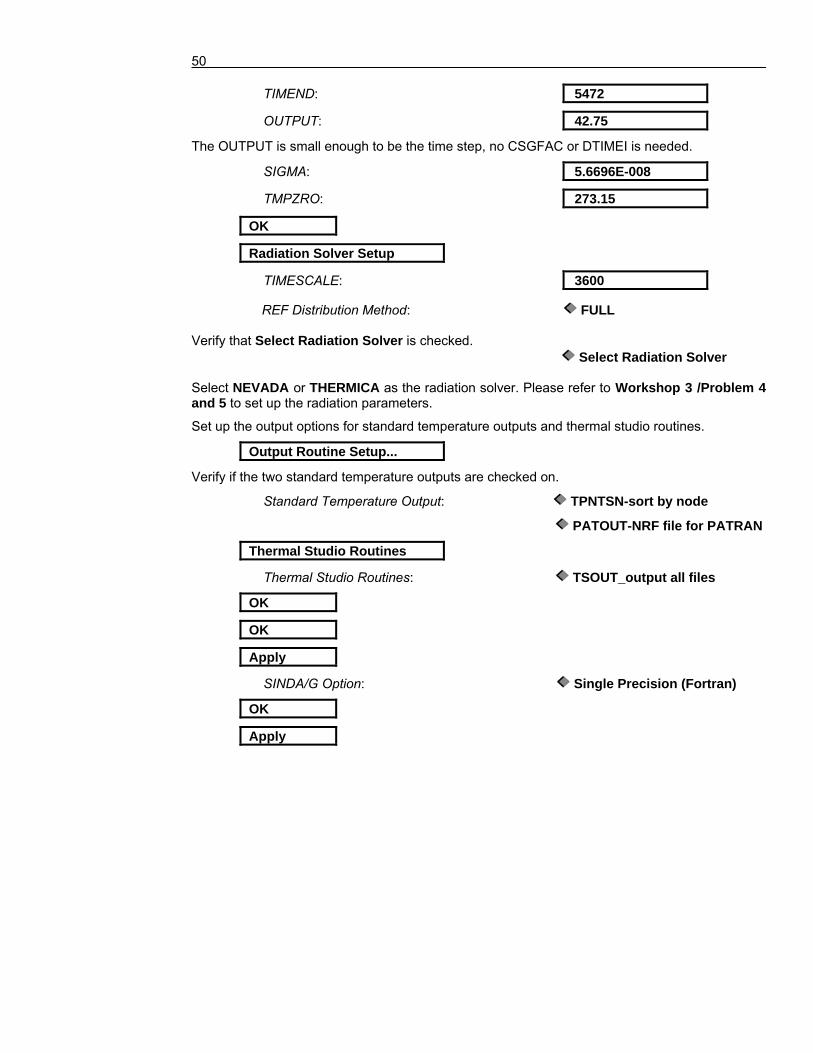
50
TIMEND: 5472
OUTPUT: 42.75
The OUTPUT is small enough to be the time step, no CSGFAC or DTIMEI is needed.
SIGMA: 5.6696E-008
TMPZRO: 273.15
OK
Radiation Solver Setup
TIMESCALE: 3600
REF Distribution Method: FULL Verify that Select Radiation Solver is checked. Select Radiation Solver Select NEVADA or THERMICA as the radiation solver. Please refer to Workshop 3 /Problem 4 and 5 to set up the radiation parameters.
Set up the output options for standard temperature outputs and thermal studio routines.
Output Routine Setup...
Verify if the two standard temperature outputs are checked on.
Standard Temperature Output: TPNTSN-sort by node
PATOUT-NRF file for PATRAN
Thermal Studio Routines
Thermal Studio Routines: TSOUT_output all files
OK
OK
Apply
SINDA/G Option: Single Precision (Fortran)
OK
Apply

SINDA/G for Patran Workshop 8 51
The NEVADA or THEMICA window will pop up depending on which radiation solver is selected. Follow the similar steps of Workshop 3 /Problem 4 and 5 to set up the orbital parameters and run radiation codes. The following result is based on Thermica radiation solver. SINDA/G will continue to calculate temperature results. 6. Access Result and Display Repeat step 9 and 10 of problem 1. There are many transient result cases available. The following picture shows the temperature result at the last orbital position. 7. Plot temperature curves in Thermal Studio
Analysis
Action: Thermal Studio
Verify the Job Name is mli_orbit.
Job Name: mli_orbit
Apply
If you repeatedly call Thermal Studio to post-process new results using the same job name, a pop up window will ask if you want to overwrite the existing project file. Click Yes to overwrite. The Thermal Studio GUI will open as follows:

52
On the left side of the thermal studio window, double click the Input icon, you will see the mli_orbit.sin file. The following is a part of the mli_orbit.sin file. BCD 3NODE DATA 1, 0.000000 , 594.0000 2, 0.000000 , 594.0000 3, 0.000000 , 594.0000 4, 0.000000 , 594.0000 C Arithmetic nodes due to MLI application and solved radiation 5, 0.000000 , -1.000000 6, 0.000000 , -1.000000 7, 0.000000 , -1.000000 8, 0.000000 , -1.000000 C Boundary nodes created by the translator -9, -273.1500 , 0.000000 END BCD 3SOURCE DATA C Heat sources from orbital environment PER 5,A1,A2, 0.2500000 ,0.00, 5472.70 PER 6,A1,A2, 0.2500000 ,0.00, 5472.70 PER 7,A1,A2, 0.2500000 ,0.00, 5472.70 PER 8,A1,A2, 0.2500000 ,0.00, 5472.70 END
SINDA/G for Patran Workshop 8 53
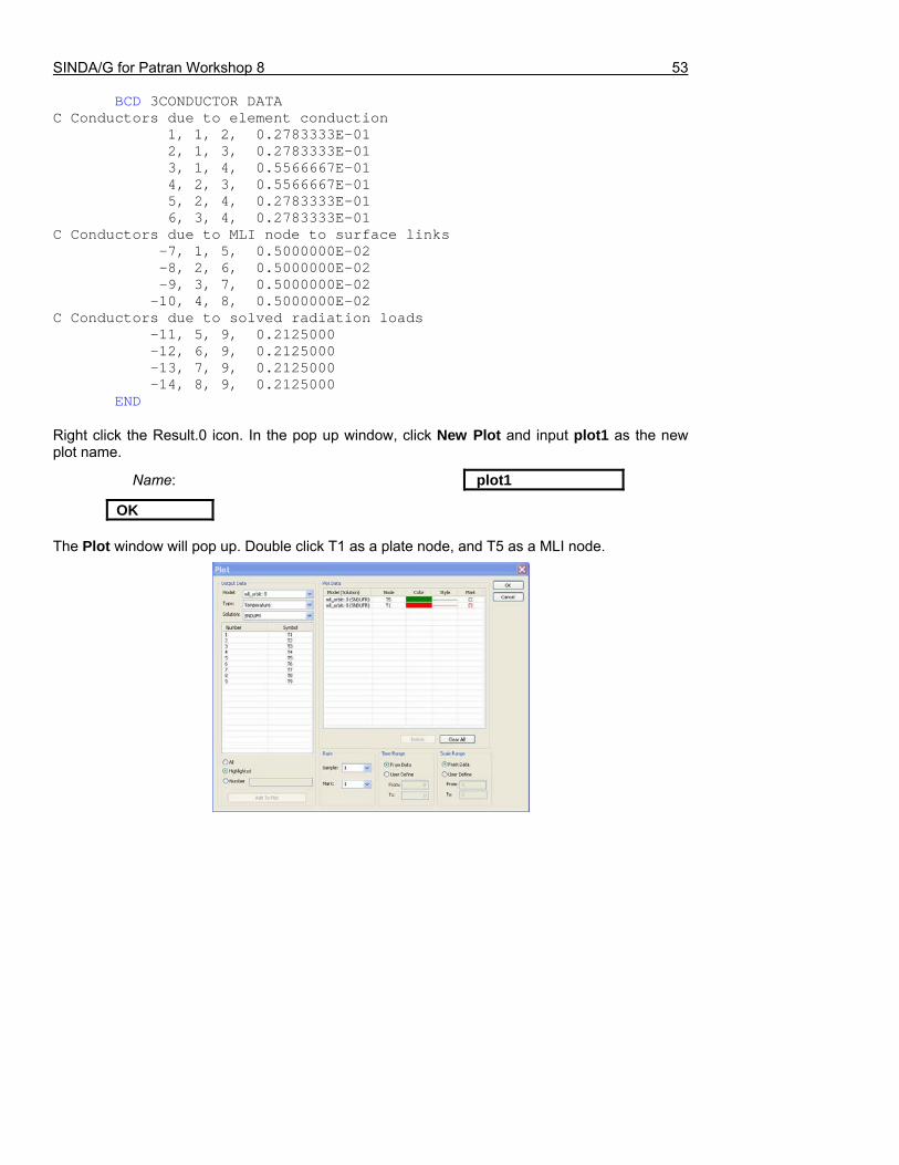
BCD 3CONDUCTOR DATA C Conductors due to element conduction 1, 1, 2, 0.2783333E-01 2, 1, 3, 0.2783333E-01 3, 1, 4, 0.5566667E-01 4, 2, 3, 0.5566667E-01 5, 2, 4, 0.2783333E-01 6, 3, 4, 0.2783333E-01 C Conductors due to MLI node to surface links -7, 1, 5, 0.5000000E-02 -8, 2, 6, 0.5000000E-02 -9, 3, 7, 0.5000000E-02 -10, 4, 8, 0.5000000E-02 C Conductors due to solved radiation loads -11, 5, 9, 0.2125000 -12, 6, 9, 0.2125000 -13, 7, 9, 0.2125000 -14, 8, 9, 0.2125000 END Right click the Result.0 icon. In the pop up window, click New Plot and input plot1 as the new plot name.
Name: plot1
OK The Plot window will pop up. Double click T1 as a plate node, and T5 as a MLI node.

54
The selected result will show up in the Plot Data list box. You can always change the curve color by clicking the color bar. Then you can click OK to plot the temperature curve in Thermal Studio.
OK
The red curve shows the temperature of the plate node. The temperature is pretty stable because the plate node has a relatively big thermal mass, also because the heat flux to the plate node is more stable because of MLI protection. Its temperature will go down very slowly until it reaches the dynamic thermal balance.The green curve shows the temperature of the MLI node. The MLI outer surface has almost no thermal mass, therefore the MLI temperature almost totally depends on the orbital heat flux. In the shadow positions, the MLI surface only receives the earth IR emission, and the temperature is pretty low. Just before entering the shadow or just after leaving the shadow (called eclipse points), the MLI surface is exposed to Sun light, therefore the curve goes up at 2 eclipse points. If you calculate more orbital positions, the two highest points should have almost the same value. Remember we only output the temperature results per 42.75 seconds. It is almost impossible to output temperatures exactly at the two eclipse points. Then after brief exposure to sunlight, the MLI surface can only receive the Earth Albedo and Earth IR emission, because only the side of the plate that is thermally insulated is exposed to the sun. The curved part of the green curve shows the MLI temperature fluctuates as the Earth Albedo changes. The Earth IR emission is supposed to be constant. 8. Close Thermal Studio and quit Patran database Close the Thermal Studio window by clicking the X button at upper right corner or click the File/Exit.

SINDA/G for Patran Workshop 8 55
File/Exit.. To complete this exercise, close the database and quit Patran. File/Quit... *************************************************************************************************** Congratulations! You have successfully completed Workshop 8 of SINDA/G for Patran. If you have any comments or questions please do not hesitate to contact us.
Network Analysis, Inc. 4151 W. Lindbergh Way, Chandler, AZ 85226 Phone 480-756-0512 Fax 480-820-1991 [email protected] www.sinda.com