Embed Size (px)
Citation preview

J Intell Robot SystDOI 10.1007/s10846-014-0029-6
6-DoF Low Dimensionality SLAM (L-SLAM)
Nikos Zikos · Vassilios Petridis
Received: 7 May 2013 / Accepted: 22 January 2014© Springer Science+Business Media Dordrecht 2014
Abstract In this paper, a new Simultaneous Local-ization and Mapping (SLAM) method is proposed,called L-SLAM, which is a Low dimension versionof the FastSLAM family algorithms. L-SLAM usesa particle filter of lower dimensionality than Fast-SLAM and achieves better accuracy than FastSLAM1.0 and 2.0 for a small number of particles. L-SLAM is suitable for high dimensionality problemswhich exhibit high computational complexity like 6-dof 3D SLAM. Unlike FastSLAM algorithms whichuse Extended Kalman Filters (EKF), the L-SLAMalgorithm updates the particles using linear Kalmanfilters. A planar SLAM problem of a rear drive car-likerobot as well as a three dimensional SLAM problemwith 6-dof of an airplane robot is presented. Experi-mental results based on real case scenarios using theCar Park and Victoria Park datasets are presented forthe planar SLAM. Also results based on simulatedenvironment and real case scenario of the Koblenzdatasets are presented and compared with the threedimensional version of the FastSLAM 1.0 and 2.0.The experimental results demonstrate the superiorityof the proposed method over FastSLAM 1.0 and 2.0.
N. Zikos (�) · V. PetridisDepartment of Electrical and Computer Engineering,Aristotle University of Thessaloniki, Thessaloniki, Greecee-mail: [email protected]
V. Petridise-mail: [email protected]
Keywords SLAM · L-SLAM · FastSLAM ·Dimensionality reduction
1 Introduction
The problem of Simultaneous Localization And Map-ping (SLAM) is vital in case of autonomous robotsand vehicles navigating in unknown environments [18,20]. Usually the map consists of a sequence of features(or landmarks), each one of which represents the posi-tion of an obstacle or a part of an obstacle (i.e. a bigobstacle can be represented by many features).
Although the Extended Kalman Filter (EKF) waswidely used for many years in the SLAM prob-lem [19], it has the disadvantage that the computa-tional cost increases significantly with the numberof features. In the early 2002 Montemerlo et al. [6–9] presented a new solution to stochastic SLAM,called FastSLAM, that approaches the problem from aBayesian point of view, while many more approaches[3, 10, 11] have been proposed since then. FastSLAMseparates the state variables into two groups. Thefirst one is estimated using particle filtering whilethe second one is estimated using Extended KalmanFilter. The resulting algorithm is an instance of theRao-Blackwellized [4] particle filtering method. Thismethod reduces significantly the complexity of theproblem [18] in environments with many features.
In this paper we present the L-SLAM [14] algo-rithm (Low dimensional-SLAM) with unknown dataassociation [22]. The key idea is to sample only the

J Intell Robot Syst
robot’s orientation on each particle, in contrast to theFastSLAM algorithms that sample the orientationalong with the position of the robot. As a result wehave a reduced dimensionality particle filter. In mostkinematic models the orientation introduces nonlin-earity into the system, thus in L-SLAM the particlefiltering technique is used only for the orientation.On the other hand, the robot’s translation can bedescribed in a linear form, thus it can be estimated,along with each feature’s position, by linear Kalmanfilters as shown below. In addition to our previouswork [14, 22] the L-SLAM method is enhancedwith the Kalman Smoothing technique instead of thedistribution merging technique which was a goodapproximation. With the Kalman smoothing tech-nique it is proved (see Appendix) that the L-SLAMmethod is mathematically consistent and describesexactly the SLAM problem.
Particle filter dimensionality reduction, gives theopportunity to use fewer particles while we can attainthe same accuracy. This reduction is more welcomewhen we are dealing with problems of high dimen-sionality. SLAM algorithms in the three dimensionalspace are computationally costly [13], because sixdimensions (three for the robot’s translation and threefor its orientation) are required. In contrast to Fast-SLAM, L-SLAM reduces the dimensionality by three,resulting thus in reduction of the complexity and thecomputational cost.
In this paper we present the planar version ofthis method, in order to compare it with the planarFastSLAM 1.0 and 2.0 algorithms. Also we presentthe extension of the L-SLAM algorithm to the threedimensional space. We present the 3-D version of thismethod, in order to compare it with the 3-D version ofthe FastSLAM 1.0 [1] and 2.0.
2 System Description
When mobile robots move in an unknown terrain withobstacles, the perception of the robot’s environmentis crucial in order to interact with it. Thus, a vari-ety of techniques were proposed. Such techniquesare the SLAM methods which try to recover the ter-rain’s map and the robot’s pose using sensor datafrom measurements and control inputs. In these meth-ods the map is considered as a set of features � =[θ1, θ2, ...., θN ] each one corresponding to an obsta-cle or a specific point of the environment (Fig. 2).
The robot’s path is represented by a time-series of it’stranslation pt = [p1, p2, ...pt ] and a time-series ofit’s orientation ϕt = [ϕ1, ϕ2, ..., ϕt ] or heading direc-tion with respect to a global axis system. In a planarproblem each feature θi (eg. θi = [θx,iθy,i]T in pla-nar SLAM and θi = [θx,iθy,iθz,i]T in 3D SLAM) isa vector with entries the Cartesian coordinates of theobstacle. Robot’s translation pt (eg. pt = [px,tpy,t ]Tin planar SLAM and pt = [px,tpy,tpz,t ]T in 3DSLAM) is a vector with entries the position at time t
while ϕt represents the angle of the robot’s orientationat time t with respect to a global axis system.
2.1 Planar Model
In this paper a rear wheel drive model of a real casescenario is presented. The mechanical characteristicsof the robotic car are derived from the CarPark - Vic-toria Park experiment [12]. In Fig. 1 the mechanicalcharacteristics of the car and the sensor are presented.
The kinematic model of the rear drive car-like robotis given in Eq. 1.
[px,t
py,t
ϕt
]=
⎡⎢⎢⎢⎢⎢⎢⎣
px,(t−1) + vt�t[cos(ϕt−1)− (a sin(ϕt−1)
+b cos(ϕt−1))tan(st )
L] 1
1−tan(st )HL
py,(t−1) + vt�t[sin(ϕt−1)+ (a cos(ϕt−1)
−b sin(ϕt−1))tan(st )
L] 1
1−tan(st )HL
ϕ(t−1) + vt�ttan(st )
L−H tan(st )
⎤⎥⎥⎥⎥⎥⎥⎦
(1)
where vt is the robot’s velocity at time t , st is thesteering angle at time t , L is the distance between therobot’s axles, H is the distance of the rear wheel from
Fig. 1 Robot’s schematic with the dimensions used in the kine-matic model. The center of the robot’s coordinate system isplaced in the tip of the laser sensor

J Intell Robot Syst
the center of the rear axle, a is the displacement of thesensor from the rear axle and b is the displacement ofthe sensor from the robot’s longitudinal axis (Fig. 1).
The measurement model of a distance and bearingsensor is given by the nonlinear equations (Fig. 2):
zt =g(pt , ϕt , θn) =
=[dtσt
]=
⎡⎣
√(px,t − θx,n)2 + (py,t − θy,n)2
arctan(py,t−θy,npx,t−θx,n
)− ϕt
⎤⎦(2)
2.2 6DoF Airplane Like Model
In this paper we use a kinematic model of a vir-tual vehicle that moves in the 3D space and is drivenby three control inputs. By definition the vehicle’sheading direction matches the X axis of it’s ownaxis system. The three control inputs consist of thelinear velocity (perpendicular to the local X axis),the rotational rate around the local X axis (roll) andthe rotational rate around the local Y axis (pitch)(Fig. 3). It is worth noting that this kinematic model isan approximation of an airplane’s kinematic model.
The measurement model corresponds to a threedimensional laser scanning sensor. An observed fea-ture is represented in a spherical coordinate system.Thus a transformation is necessary in order to obtainthe feature’s position in a Cartesian form and back-wards.
Fig. 2 The robot coordinate system and the position of θi land-mark with respect to the robot coordinate system OR . θ is theangle between the vectors XR and ORθ
Fig. 3 The robot’s coordinate system in the three dimensionalspace. The three control inputs consist of the linear velocity(perpendicular to the local X axis), the rotational rate aroundthe local X axis (roll) and the rotational rate around the local Yaxis (pitch)
2.2.1 Kinematic Model
The kinematic model in the three dimensional spaceis much more complicated than the one in the twodimensional space. In this multidimensional space themost difficult problem is the calculation of the ori-entation of the robot. The kinematic model, whichis described below, is based on the concept of thetranslation-rotation, due to its mathematical simplic-ity.
The kinematic model is given by:
⎧⎪⎪⎨⎪⎪⎩px,t
py,t
pz,t
Rt
⎫⎪⎪⎬⎪⎪⎭ =
⎧⎪⎪⎨⎪⎪⎩px,(t−1) + vt cos(bt−1) cos(ct−1)�t
py,(t−1) + vt cos(bt−1) sin(ct−1)�t
pz,(t−1) − vt sin(bt−1)�t
Rt−1RotY (ωy,t�t)RotX(ωx,t�t)
⎫⎪⎪⎬⎪⎪⎭(3)
where Rt is the robot’s rotation matrix, vt is the linearvelocity, ωx,t ,ωy,t are the rotational rates around the Xand Y axis respectively and a, b, c are the XYZ Eulerangles of the vehicle’s orientation with respect to theglobal axis system. RotY (.) and RotX(.) refer to therotation matrices rotating a vector around the Y andX axis respectively. The Euler angles are given by theEq. 4.
at = atan2(Rt,(3,2), Rt,(3,3))
ct = atan2(Rt,(2,1), Rt,(1,1))
bt = atan2(−Rt,(3,1), cos(ct )Rt,(1,1)+ sin(ct )Rt,(2,1))
(4)
where Rt,(i,j) is the element corresponding to the ith
row and the j th column on the rotation matrix Rt .

J Intell Robot Syst
2.2.2 Measurement Model
The measurement model corresponds to a threedimensional laser scanning sensor, which measuresthe distance and the direction of an observed feature.The spherical coordinate system is used (Fig. 4).
The spherical to Cartesian coordinate system trans-formation is described by the equation below.
θRi =⎡⎣ θRx,iθRy,iθRz,i
⎤⎦ =
⎡⎣ di cos(σ2,i ) cos(σ1,i)
di cos(σ2,i ) sin(σ1,i )
di sin(σ2,i )
⎤⎦ (5)
where di is the Euclidean distance between the sen-sor and the observed feature θi and σ1,i and σ2,i arethe angular displacements from the positive x-axis andfrom the x-y plane, respectively.
The resulting position refers to the robot’s local axissystem, thus a transformation (6) is necessary in orderto obtain its global position.
θi = RtθRi + Pt (6)
θi = [θx,iθy,iθz,i]T is the feature’s position in theglobal axis system, θRi is the features position in therobot’s axis system and Pt = [px,tpy,tpz,t ]T andRt is the robot’s position vector and rotation matrixrespectively.
The inverse measurement model is given by theequations:
σ1 = atan2(θRy,i, θRx,i)
σ2 = atan2
(θRz,i,
√θRx,i
2 + θRy,i2)
(7)
d =√θRx,i
2 + θRy,i2 + θRz,i
2
Fig. 4 The measurement model of a three dimensional laserscanner sensor
where the feature’s coordinates relative to the robot’sframe coordinates are obtained from the equation:
θRi = R−1t (θi − Pt) (8)
3 Planar L-SLAM with Unknown DataAssociation
Most of the SLAM algorithms calculate variants of thefollowing posterior probability distribution:
f (pt , ϕt , �|zt , ut , nt ) (9)
where zt = [z1, z2, ....zt ] is a time-series of mea-surements produced by measuring instruments (e.g.laser sensors produce a sequence of distance and bear-ing measurements of the visible obstacles). Vectornt = [n1, n2, ...nt ] is a time-series of indexes such thatindex nj , j = 1..t matches the observation zj to thecorresponding feature θnj . Vector ut = [u1, u2, ...ut ]is the time-series of the robot’s control vectors (e.g.linear velocity and steering angle).
In the L-SLAM algorithm a different factorizationof the posterior (9) is proposed:
f (pt , ϕt , �|zt , ut , nt ) =f (ϕt |zt , ut , nt )f (pt , θnt |ϕt , zt , ut , nt )
f (pt−1, θi �=nt |pt , θnt , ϕt , zt , ut , nt )
(10)
This factorization states that current features’ posi-tions and robot’s position can be calculated indepen-dently as long as the robot’s orientation is known. Thisfactorization consists of three factors corresponding toparticle filter (Section 3.1), Kalman filter (Section 3.2)and Kalman smoothing (Section 3.3) subsequently Itis noteworthy that this factorization is exact and it’sderivation can be found in Appendix.
3.1 Particle Filter
The first step of the L-SLAM algorithm is the robot’sorientation drawing process for every particle. Eachparticle at time t − 1 and the control input at time t
are used to generate a probabilistic guess of the new

J Intell Robot Syst
angle (11) using the robot’s kinematic model (1) forthe orientation (12).
ϕit ∼ f (ϕ|ϕi
t−1, ut ) (11)
ϕit = ϕi
(t−1) + vit �ttan(sit )
L−H tan(sit )(12)
where vit , sit are drawn for each particle i using the
measured values vt , st and their noise characteristics.It is noteworthy that the distribution of the anglesdepends only on control noise and not measurementnoise.
3.2 Kalman Filter
In contrast to the FastSLAM algorithms in which theEKF estimate a two dimensional state vector (the twodimensions of the feature’s position), we propose astate vector μ of four states, that include the robot’sand the feature’s positions.
μi,jt =
⎡⎢⎢⎢⎣pi,jx,t
pi,jy,t
θi,jx,t
θi,jy,t
⎤⎥⎥⎥⎦ =
⎡⎢⎢⎢⎢⎢⎢⎢⎢⎢⎢⎣
pi,j
x,t−1 + vit �t[cos(ϕit−1)− (a sin(ϕi
t−1)
+b cos(ϕit−1))
tan(sit )L
] 11−tan(sit )
HL
pi,j
y,t−1 + vit �t[sin(ϕit−1)+ (a cos(ϕi
t−1)
−b sin(ϕit−1))
tan(sit )L
] 11−tan(sit )
HL
θi,j
x,t−1
θi,j
y,t−1
⎤⎥⎥⎥⎥⎥⎥⎥⎥⎥⎥⎦
(13)
where p is the robot’s position, v is the robot’s veloc-ity, ϕ is the robot’s heading angle (orientation) andθ is the feature’s position. The super-script i corre-sponds to the ith particle while the super-script j
corresponds to the j th feature. The subscript t refersto time instance t .
Using Eq. 13 we can write the state transition modelin a linear form:
μi,jt = Fμ
i,j
t−1 + Buit + νi,jt (14)
where
F = I, B
⎡⎢⎢⎣�t 00 �t
0 00 0
⎤⎥⎥⎦
and
uit =
⎡⎢⎢⎣ vit
[cos(ϕit−1)−(a sin(ϕit−1)+b cos(ϕit−1))tan(sit )
L ]1−tan(sit )
HL
vit[sin(ϕit−1)+(a cos(ϕit−1)−b sin(ϕit−1))
tan(sit )L ]
1−tan(sit )HL
⎤⎥⎥⎦
where νit ∼ N(
0,Qi,jν,t
)is the state noise vector.
The robot’s input control vector involves noisesv = v + ε1 where v is the velocity command and v
is the actual velocity. Then the noise vector ν of thetransition state model (14) is a Gaussian noise vectorthat depends on the robot’s heading angle, as shown inEq. 15.
νit =
⎡⎢⎢⎢⎢⎢⎢⎣
ε1[cos(ϕit−1)−(a sin(ϕit−1)+b cos(ϕit−1))
tan(sit )L ]
1−tan(sit )HL
ε1[sin(ϕi
t−1)+(a cos(ϕit−1)−b sin(ϕi
t−1))tan(sit )
L]
1−tan(sit )HL
00
⎤⎥⎥⎥⎥⎥⎥⎦
(15)
As measured quantities we use the relative positionof each feature with respect to the robot’s position. Asshown in Eq. 16, for the calculation of this relativeposition we use the distance and bearing measure-ments combined with the robot’s orientation. Theangle of the robot’s orientation is generated by thedrawing method as described above (11, 12).
zi,jt =
[�x
i,jt
�yi,jt
]=
[θi,jx,t − p
i,jx,t
θi,jy,t − p
i,jy,t
](16)
=[djt cos(ϕi
t + σjt )
djt sin(ϕi
t + σjt )
]
where d is the feature’s actual distance from the sensorand σ is the actual bearing of the feature.
Using Eq. 16 we can write the linear measurementmodel,
zi,jt = Hμ
i,jt +ξ
i,jt =
[−1 0 1 00 −1 0 1
]μi,jt +ξ
i,jt (17)
where ξ i,jt ∼ N(0,Qi,jξ,t ) is the linearized noise vector
corresponding to the instrument’s noise vector, whichis described below.
The instrument’s measurements are noisy d =d + ε3,σ = σ + ε4 where d, σ are the measured

J Intell Robot Syst
ones and d, σ are the actual ones. Using the noisymeasurements Eq. 16 becomes
zi,jt =
[(d
jt + ε3) cos(ϕi
t + σjt + ε4)
(djt + ε3) sin(ϕi
t + σjt + ε4)
]
=
⎡⎢⎢⎢⎢⎣
djt cos(ϕi
t + σjt ) cos(ε4)− d
jt sin(ϕi
t + σjt ) sin(ε4)
+ε3 cos(ϕit + σ
jt ) cos(ε4)− ε3 sin(ϕi
t + σjt ) sin(ε4)
djt sin(ϕi
t + σjt ) cos(ε4)+ d
jt cos(ϕi
t + σjt ) sin(ε4)
+ε3 sin(ϕit + σ
jt ) cos(ε4)+ ε3 cos(ϕi
t + σjt ) sin(ε4)
⎤⎥⎥⎥⎥⎦
For small amounts of measurement noises (ε3, ε4)we can use the approximations sin(ε4) ≈ ε4,cos(ε4) ≈ 1 and ε3 sin(ε4) ≈ 0. Thus the measure-ment Eq. 16 becomes:
zi,jt =
[�x
i,jt
�yi,jt
]+ ξ
i,jt =
[djt cos(ϕi
t + σjt )
djt sin(ϕi
t + σjt )
]+ ξ
i,jt
where
ξi,jt =
[ε3 cos(ϕi
t + σjt )− d
jt ε4 sin(ϕi
t + σjt )
ε3 sin(ϕit + σ
jt )+ d
jt ε4 cos(ϕi
t + σjt )
]
(18)
The modern distance-bearing instruments (e.g.laser sensors) have small measurement noises. There-fore the noise vector ξ
i,jt can be approximated sat-
isfactorily by a Gaussian noise vector with zeromean and a covariance matrix Q
i,jξ,t , which is calcu-
lated through ξi,jt using standard statistic techniques.
ξ is a function of the noises’ standard deviationsstd(ε3), std(ε4), the measurements d
jt , σ
jt and the
robot’s heading angle ϕit .
Using the Eqs. 14, 15, 17, 18 we can derive theinnovation matrix Z and the innovation residual y of aKalman filter (19)
μi,jt = Fμ
i,j
t−1 + Buit
�i,j
t |t−1 = F�i,j
t−1FT +Q
i,jν,t (19)
yi,jt = z
i,jt −Hμ
i,jt
Zi,jt = H�
i,j
t |t−1HT +Q
i,jξ,t
which leads us to the calculation of the importancefactor wi,j
t (20).
wi,jt =
∣∣∣2πZi,jt
∣∣∣− 12
exp
(−1
2yi,jt
TZi,jt
−1yi,jt
)(20)
For a given measurement zt we calculate N dif-ferent importance factors, one for every particle. Thisprocedure is used to determine the data association,i.e. the feature that matches best to the observation.This is the most popular solution to the data asso-ciation problem. The solution is the index nt thatmaximizes the likelihood of the measurement [21].
nt = argmaxnt (p(zt |nt , nt−1, pt , ϕt , ut , zt−1)) (21)
The importance factor is usually referred to aslikelihood [21], thus the Eq. 21 can be expressed as
nit = argmaxj (wi,jt ) (22)
After finding the associated data, the next step isto update the corresponding feature in every particle.The mean and the covariance of the state vector arecalculated through the Kalman filter update equations(23).
Ki,nitt = �
i,nitt |t−1HZ
i,nitt
−1(23)
μi,nitt = μ
i,nitt +K
i,nitt y
i,nitt
�i,nitt = (I −K
i,nitt H )�
i,nitt |t−1
These update equations are calculated indepen-dently for every particle. It is noteworthy, that theEq. 22 will always return an associated datum nomatter how well the features fits to the observation.Thus a common technique is to compare the maxi-mum importance factor max(w
jt ) with a predefined
threshold which determines whether the observationcorresponds to a new unobserved feature or not. Incase of a new feature, its estimated position is includedin the feature set �.
The importance factor measures the angle accu-racy of the robot’s orientation, which is drawn in thesampling process, based on the instrument’s measure-ments. Thus the importance factor of every particle

J Intell Robot Syst
can be generated by the product (24) of the past factorsmultiplied by the new one.
wit = wi
t−1wi
nitna (24)
3.3 Kalman Smoothing
In addition to our previous work [14, 22] in thispaper the L-SLAM method is enhanced using Kalmansmoothing algorithms [2, 15–17]. With Kalmansmoothing it is possible to transfer all the informationfrom new observations backwards in order to updatethe past time robot’s time series position and the restof the map. It is an iterative procedure that starts attime t − 1 and updates the states going backwards.
The covariance matrix P t1|t2 represents the covari-ance of the robot’s position and the feature’s positionat time t1 with respect of the measurements up totime t2 (25). Subsequently this matrix is composedfrom the robot’s position covariance sub matrix P
t1|t2p ,
the feature’s position covariance sub matrix Pt1|t2θ and
the covariance sub matrix Pt1|t2p,θ which describes the
correlation between them.
P t1|t2 =[P
t1|t2p P
t1|t2p,θ
Pt1|t2θ,p P
t1|t2θ
](25)
The backwards Kalman gain [2, 16] as derived fromthe Eq. 26, is calculated from the robot’s positioncovariance matrices and refers only in the gain appliedin the robot’s position at time t − 1 with respect of theobservation at time t .
Kt−1|tp = P t−1|t−1
p (P t−1|t−1p +Qt−1)
−1
(P t |tp − P t−1|t−1
p −Qt−1)(Pt−1|t−1p +Qt−1)
−1 (26)
Subsequently, the innovation residual [2, 16] iscalculated by Eq. 27.
yt−1|t = (P t−1|t−1p +Qt−1)
(P t |tp − P t−1|t−1
p −Qt−1)−1(μt |t − μt−1|t−1 − But)
(27)
Any observation of the feature θnt−1 at time t − 1is correlated with the corresponding robot’s positionpt−1. Thus the feature’s Kalman gain is a function of
the robot’s position Kalman gain Kt−1|tp and covari-
ance matrixP t−1|t−1p and the robot’s - feature’s covari-
ance matrix Pt−1|t−1p,θ . This is combined in a single
Kalman gain that contains both robot’s and feature’sposition gains (28). This gain along with the innova-tion residual (27) transfers all the information of theobservation at time t backwards in the position and thecorresponding feature at time t − 1.
Kt−1|t =[
Kt−1|tp
Pt−1|t−1p,θ
TK
t−1|tp
TP
t−1|t−1p
−1
](28)
Since the Kalman gain and the innovation residualare calculated, the smoothed instances of the robot’sposition, the feature’s position and their covariances attime t − 1 are applied using Eqs. 29 and 30.
μt−1|t = μt−1|t−1 +Kt−1|t yt−1|t (29)
P t−1|t = (I +Kt−1|t[I
0
])P t−1|t−1 (30)
This is an iterative procedure that starts at timet − 1 through t = 0. In real case scenarios this pro-cedure has a proportional computational cost with thetime. When Q �= 0, the Kalman gain is continuouslydecreasing as this procedure goes backwards. In orderto minimize the computational cost, a threshold can
be used such as√|Kt−n|t
p | < thr , which states thathen the determinant of the gain becomes too small theKalman smoothing has no more impact and thus theprocedure can be stop.
Although the proposed approach has been pre-sented for specific models, it can be used without anymodifications for any kinematic model which has thefollowing properties:
1. the translations enter linearly in the state equa-tions,
2. the orientation angles enter nonlinearly, but forfixed angles the equations are linear,
3. and the control inputs enter either linearly, or incase they enter nonlinearly, their noises can beapproximated by an additive noise term.
4 6DoF SLAM with Unknown Data Association
In this section we extend the L-SLAM algorithm tothe three dimensional space. Thus we use a kinematic

J Intell Robot Syst
model of a virtual vehicle that moves in the 3D spaceand is driven by three control inputs. By definition thevehicle’s heading direction matches the X axis of it’sown coordinate system. The three control inputs con-sist of the linear velocity (along to the local X axis),the rotational rate about the local X axis (roll) andthe rotational rate about the local Y axis (pitch). Thiskinematic model is an approximation of an airplane’skinematic model.
4.1 L-SLAM Algorithm with Unknown DataAssociation
In the 6-dof case the Eq. 9 becomes:
f (pt , Rt , �|zt , ut , nt )= f (Rt |zt , ut , nt )f (pt , θnt |Rt , zt , ut , nt )
f (pt−1, θi �=nt |pt , θnt , Rt , zt , ut , nt )
(31)
As in the planar case, the first step of the L-SLAMalgorithm is the robot’s orientation drawing processto generate the particles. Each particle at time t − 1and the control input at time t are used to generate aprobabilistic estimate of the new rotation matrix (32)using the robot’s orientation kinematic model given byEq. 33 (which is the last line in Eq. 3).
Rit ∼ f (R|Ri
t−1, ut ) (32)
Rit = Ri
t−1RotY (ωiy,t�t)RotX(ωi
x,t�t) (33)
where ωix,t and ωi
y,t are drawn for each particle i usingthe measured values ωx,t for the roll and ωy,t for thepitch and their noise characteristics. It is noteworthythat the distribution of the angles depends only oncontrol noise and not on measurement noise.
In contrast to the FastSLAM algorithms, in whichthe EKF has three state variables (the three dimensionsof the feature’s position), we propose a state vectorof six states μ, which includes the robot’s and thefeature’s position.
μi,jt =
⎡⎢⎢⎢⎢⎢⎢⎢⎣
pi,jx,t
pi,jy,t
pi,jz,t
θi,jx,t
θi,jy,t
θi,jz,t
⎤⎥⎥⎥⎥⎥⎥⎥⎦=
⎡⎢⎢⎢⎢⎢⎢⎢⎢⎣
pix,(t−1) + vt cos(bi
t−1) cos(cit−1)�t
piy,(t−1) + vt cos(bi
t−1) sin(cit−1)�t
piz,(t−1) − vt sin(bi
t−1)�t
θi,j
x,t−1
θi,j
y,t−1
θi,j
z,t−1
⎤⎥⎥⎥⎥⎥⎥⎥⎥⎦
(34)
where p is the robot’s position, v is the actual robot’svelocity, a, b, c are the robot’s orientation expressedas XYZ Euler angles and θ is the feature’s position.The super-script i refers to the ith particle while thesuper-script j refers to the j th feature. The subscript trefers to time instance t .
Using Eq. 34 we can describe the state transitionmodel in a linear form:
μi,jt = Fμi
t−1 + But + νit (35)
where
F = I, B =
⎡⎢⎢⎢⎢⎢⎢⎣
�t 0 00 �t 00 0 �t
0 0 00 0 00 0 0
⎤⎥⎥⎥⎥⎥⎥⎦
ut =⎡⎣ vt cos(bit−1) cos(cit−1)
vt cos(bit−1) sin(cit−1)
vt sin(bit−1)
⎤⎦
and νit ∼ N(0,Qiν,t ) is the noise vector. The robot’s
input control vector involves noises: vt = vt + ε1
where vt is the velocity command and vt is the actualvelocity. Then the noise vector νt of the transition statemodel (35) is a Gaussian vector that depends on therobot’s heading angle, as shown in Eq. 36.
νit =
⎡⎢⎢⎢⎢⎢⎢⎣
ε1 cos(bit−1) cos(cit−1)�t
ε1 cos(bit−1) sin(cit−1)�t
ε1 sin(bit−1)�t
000
⎤⎥⎥⎥⎥⎥⎥⎦
(36)
As measured quantities we use the relative positionof each feature with respect to the robot’s position. Asshown in Eq. 37, in order to calculate this relative posi-tion we use the distance and bearing measurementscombined with the robot’s rotation matrix. The angleof the robot’s orientation is generated by the drawingmethod as described above (32, 33).
⎡⎢⎣�x
i,jt
�yi,jt
�zi,jt
⎤⎥⎦ =
⎡⎢⎣ θ
i,jx,t − p
i,jx,t
θi,jy,t − p
i,jy,t
θi,jz,t − p
i,jz,t
⎤⎥⎦ = Ri
t θRi (37)

J Intell Robot Syst
where Rit is the robot’s rotation matrix correspond-
ing to the ith particle at time t and θRi is the feature’sposition as obtained through the transformation (5).
The instrument’s measurements σ1, σ2, d are noisy:σ1 = σ1 + ε4,σ2 = σ2 + ε5,d = d + ε6 whereσ1, σ2, d are the measured ones and σ1, σ2, d are theactual ones.
For relative small amounts of measurement noises(ε4, ε5, ε6) we can use the approximations sin(εi) ≈εi and cos(εi) ≈ 1 and εiεj ≈ 0. Thus the measure-ment Eq. 37 becomes:
zi,jt = Hμ
i,jt + ξ
i,jt = (38)
=⎡⎣−1 0 0 1 0 0
0 −1 0 0 1 00 0 −1 0 0 1
⎤⎦μ
i,jt + ξ
i,jt
where
ξi,jt = Ri
t
⎡⎢⎢⎢⎢⎣
ε6 cos(σ2) cos(σ1)+ ε5d cos(σ1) sin(σ2)
+ ε4d cos(σ2) sin(σ1)ε6 cos(σ2) sin(σ1)+ ε5d sin(σ1) sin(σ2)
+ ε4d cos(σ2) cos(σ1)ε6 sin(σ2)+ ε5d cos(σ2)
⎤⎥⎥⎥⎥⎦
(39)
The noise vector ξi,jt can be satisfactorily approxi-
mated by a Gaussian with zero mean and a covariancematrix Q
i,jξ,t . The covariance matrix Q
i,jξ,t can be calcu-
lated through ξi,jt using standard statistic techniques.
Also it is a function of the noises’ standard devi-ations std(ε4), std(ε5), std(ε6), the measurementsσj
1,t , σj
2,t , djt and the robot’s rotation matrix Ri
t .Using the Eqs. 35, 36, 38, 39 we can derive the
innovation matrix Z and the residual y of a Kalmanfilter (40)
μi,jt = Fμ
i,j
t−1 + Buit
�i,j
t |t−1 = F�i,j
t−1FT +Q
i,jν,t (40)
yi,jt = z
i,jt −Hμ
i,jt
Zi,jt = H�
i,j
t |t−1HT + S
i,jξ,t
which leads us to the calculation of the importancefactor wi,j
t (41).
wi,jt =
∣∣∣2πZi,jt
∣∣∣− 12
exp(−1
2yi,jt
TZi,jt
−1yi,jt ) (41)
For a given measurement zt we calculate N dif-ferent importance factors one for every particle. This
procedure is used to determine the data association,i.e. the feature that matches best to the observation.This is the most popular solution to the data asso-ciation problem. The solution is to choose the indexnt that maximizes the likelihood of the measurement[21].
nt = argmaxnt (p(zt |nt , nt−1, pt , Rt , ut , zt−1))
(42)
The importance factor is usually referred to as like-lihood [21], thus the Eq. 42 can be expressed as
nit = argmaxj (wi,jt ) (43)
After finding the associated data, the next step isto update the corresponding feature in every particle.The mean and the covariance of the state vector arecalculated through the Kalman filter update Eq. 44.
Ki,nitt = �
i,nitt |t−1HZ
i,nitt
−1(44)
μi,nitt = μ
i,nitt +K
i,nitt y
i,nitt
�i,nitt = (I −K
i,nitt H )�
i,nitt |t−1
These update equations are calculated indepen-dently for every particle. It is noteworthy, that theEq. 43 will always return an associated feature nomatter how much the feature fits to the observation.Thus a common technique is to compare the maxi-mum importance factor max(w
jt ) with a predefined
threshold which determines whether the observationcorresponds to a new unobserved feature or not. Incase of a new feature, its estimated position is includedin the feature set �.
4.2 L-SLAM Algorithm in Summary
A pseudocode of the L-SLAM algorithm withunknown data association and multiple observationsper iteration is given below.
BEGIN L-SLAM(St−1, zt , ut )for i = 1 : M particles do
draw Rit ∼ prob(R|Ri
t−1, ut )
for j = 1 : Nt features doμ = Fμi
j + Bu
�ij = F�i
jFT +Qν,t

J Intell Robot Syst
Z = H�ijH
T +Qξ,t
wi,jt = |2πZ|− 1
2 exp(− 12 y
T Z−1y)
end fornit = argmaxj (w
i,jt )
if max(wi,ni
t ) < p0 feature is new thenj = N + 1μij : initialize mean
�ij : initialize covariance matrix
elseK = �i
nitHZ−1
μi
nit= μ+Ky
�i
nit= (I −KH)�i
nitend ifKalman Smoothingfor k = t − 1 : 1 do
Calculate yk|t Eq. 27Calculate Kk|t Eq. 28μk|t = μk|k +Kk|t yk|t
P k|t = (I +Kk|t [ I0])P k|k
end forwit = wi
t−1wi,nitt
end forResampleEND
5 Experiments and Results
5.1 2-D Problem
All the experiments were performed on the Car-Park(Fig. 5) and the Victoria park (Fig. 6) datasets [12]acquired from the university of Sydney. In both casesthe car was equipped with a horizontal scanninglaser sensor with 80 meters observing radius and 180degrees field of view.
The experiments were performed 20 times for eachmethod for 4,10,20 and 40 particles. Following thecalculation of each particle’s importance factor, aresampling method [5] runs as soon as the ”effectivesample size” is lower than 75 % of the particle popu-lation. Due to random sampling of every particle, theresults differ on every run. Thus, all three methods(FastSLAM 1.0, FastSLAM 2.0 and L-SLAM) were
performed 20 times in order to compare them on thebasis of the mean and the standard deviation (Fig. 7)of the robot’s position error. The results were obtainedusing Matlab in the same machine.
The results from all three methods (Fig. 7) are sum-marized in Table 1. L-SLAM appears to exhibit thesame accuracy as the FastSLAM 2.0 algorithm. Onthe other hand, the FastSLAM 1.0 method’s error ishigher than the error of the other two methods. Thecomputational cost, measured in process time, of theFastSLAM 2.0 is much higher than the L-SLAM’s,while both methods have almost the same accuracy.
In addition to the Car-Park and Victoria Parkdatasets the method was tested in a simulated envi-ronment [14]. The experiments were performed inthe same simulated environment for all three meth-ods (L-SLAM, FastSLAM 1.0 and 2.0) with differentnumber of particles. The simulated map of obstacleswas chosen to be sparse enough in order to observe theadditive error efficiently. The virtual robotic vehiclewas equipped with a horizontal scanning laser sensorwith 30 meters observing radius and 120 degrees fieldof view. In the experiments a variety in the numberof the particles was chosen, with minimum 4 particlesand maximum 40 particles and the results are summa-rized in Table 2. The performance of the algorithmson this dataset is the same as the one on the CarParkdataset.
−20 −10 0 10 20 30 40−30
−20
−10
0
10
20
30
Fig. 5 Feature map used in the Car-park dataset

J Intell Robot Syst
Fig. 6 Robot’s path and feature map in the Victoria park dataset
5.2 6-DoF Problem
5.2.1 Simulated Environment
All the experiments were performed on a simulateddataset. The virtual robotic vehicle was equipped witha 3D pan-tilt scanning laser sensor with 4 metersobserving radius and 120 degrees field of view bothon vertical and horizontal scanning. The robot’s con-trol noise was defined through the standard devia-tion of linear and angular velocity noises as σv =0.05 m/s, σωx = σωy = 1deg/s, while the observa-tion noise were σd = 0.1m, σσ = σφ = 3o.
The experiments were performed 64 times for eachmethod for 4,10,20,40 and 100 particles. Followingthe calculation of each particle’s importance factor,a resampling method [5] runs as soon as the ”effec-tive sample size” is lower than 75 % of the particlepopulation. Due to random sampling of every particle,the results differ on every run. Thus, the three meth-ods (FastSLAM 1.0, 2.0 and L-SLAM) were run 64times in order to compare them on the basis of themean of the error robot’s position error. The resultswere obtained using Matlab in the same machine. Themethods were tested on three different maneuver sets,one without loop closing and two with small and large

J Intell Robot Syst
Fig. 7 Robot’s meanposition error and standarddeviation with differentnumber of particles on theCarPark dataset
0 5 10 15 20 25 30 35 40 45 500
0.2
0.4
0.6
0.8
1
1.2
1.4
1.6
1.8
2
Particles
Rob
ot P
ositi
on E
rror
− S
tand
ard
Dev
iatio
n (m
)
FastSLAM 1.0FastSLAM 2.0L−SLAM
loops where the vehicle closes the loop i.e it revisitsan area in the map.
In the first set of experiments the vehicle covered anarea without passing from previously observed area.The vehicle covered a distance of about 20 meters,performed a variety of maneuvers and observed in
Table 1 Comparison results of all methods on the Car-Park andVictoria Park datasets with different number of particles (Planarproblem)
Algorithm Number of Time Position
particles (sec) error (m)
Car-Park
FastSLAM 1.0 4 24.1 sec 0.84 m
FastSLAM 2.0 4 86.2 sec 0.50 m
L-SLAM 4 24.9 sec 0.48 m
FastSLAM 1.0 40 270 sec 0.43 m
FastSLAM 2.0 40 739 sec 0.41 m
L-SLAM 40 283 sec 0.40 m
Victoria Park
FastSLAM 1.0 4 168.1 sec 2.49 m
FastSLAM 2.0 4 426.2 sec 0.60 m
L-SLAM 4 202.9 sec 0.68 m
FastSLAM 1.0 40 1149.7 sec 0.69 m
FastSLAM 2.0 40 2951.5 sec 0.61 m
L-SLAM 40 1640.0 sec 0.60 m
total about 160 features. The purpose of this experi-ment is to compare the cumulative error of the threemethods on the basis of the vehicle’s distance error.The mean position error (fourth column in the Table 3)is reduced as the number of particles increases forall methods, but it is noteworthy that the L-SLAMmethod converges as the number of particles increasesfaster than in FastSLAM 1.0 and 2.0. Another keyfeature of the L-SLAM method is the reduced com-putation time. The difference in the computation timeis due to the fact that in FastSLAM 1.0 and 2.0 thecomputation of the complicated 3D Jacobian matri-ces of the EKFs is required. It is noteworthy that theJacobian matrices are calculated from their analyti-cal form but nevertheless the computational cost ishigh due to the recurrent calculation for every obser-vation for every particle (eg. for 100 particles with360 distance-bearing measurements it is necessary tocalculate 36.000 Jacobian matrices from its analyticalform in every step). L-SLAM takes about one third ofFastSLAM 2.0 execution time.
Another noteworthy observation is the percentageof the resamples carried out during the simulation(sixth column of the Tables 3, 4, 5). In FastSLAM 1.0resampling is performed almost in every step due tothe fact that in 6-D space a larger number of particlesis needed. In FastSLAM 2.0 resampling percentageper iteration is smaller due to the additional recalcula-tion of the robot’s pose from the measurements. On the

J Intell Robot Syst
Table 2 Comparisonresults of all methods on theon the simulatedenvironment with differentnumber of particles (Planarproblem)
Algorithm Number of Time/step Position Features
particles (sec) error (m) error (m)
FastSLAM 1.0 4 7.1 ms 0.55 m 0.65 m
FastSLAM 2.0 4 19.0 ms 0.15 m 0.22 m
L-SLAM 4 7.9 ms 0.19 m 0.26 m
FastSLAM 1.0 40 58.0 ms 0.23 m 0.28 m
FastSLAM 2.0 40 198.0 ms 0.13 m 0.15 m
L-SLAM 40 64.0 ms 0.13 m 0.15 m
other hand, L-SLAM resampling rate is much smallerthan both FastSLAM 1.0 and 2.0 for the same numberof particles.
In the second and third sets of experiments, thevehicle completed a series of maneuver sets, with loopclosing in the end of the motion and observed about190 and 240 different features respectively. In the sec-ond set of experiments the vehicle moved once along aloop on a 3-D curve covering a distance of 32 meters.In the third experiment the vehicle also moved oncealong a loop covering a distance of 64 meters. Theseexperiments were performed in order to observe theconvergence of the particles at the moment of the loopclosing, where the vehicle enters in an already mappedarea. Tables 4 and 5 show the results for the secondand third sets of experiments respectively. The fifth
column of these tables shows the vehicle’s distanceerror at the moment of loop closing. L-SLAM methodachieves its minimum error for fewer particles thanboth FastSLAM 1.0 and FastSLAM 2.0.
In the third set of experiments, the vehicle travelsalong a long loop. In this bigger map the number ofparticles are not enough to cover the six dimensionalstate space of the FastSLAM 1.0. As the experimen-tal results show, FastSLAM 1.0 achieves its minimumerror value for 40 particles in the second set of exper-iments and 100 particles in the third set of exper-iments, while FastSLAM 2.0 achieves its minimumerror value for 20 particles in the second set of experi-ments and 40 particles in the third set of experiments.L-SLAM achieves its minimum error value for 10
Table 3 Comparisonresults among theFastSLAM 1.0, 2.0 andL-SLAM on a datasetwithout loop closing. Thevehicle moved on a 3-Dcurve covering a distance of20 meters, with variousmaneuvers
Alg. N No Time (sec) M. Pos. std Loop Cl. Res. %
error (m) error (m)
FS 1 4 0.12 0.29 m 0.12 – 97 %
FS 2 4 0.20 0.26 m 0.07 – 87 %
LS 4 0.07 0.20 m 0.06 – 10 %
FS 1 10 0.22 0.24 m 0.08 – 89 %
FS 2 10 0.42 0.20 m 0.06 – 83 %
LS 10 0.14 0.19 m 0.06 – 6 %
FS 1 20 0.36 0.19 m 0.06 – 76 %
FS 2 20 0.70 0.18 m 0.06 – 30 %
LS 20 0.20 0.18 m 0.06 – 9 %
FS 1 40 0.69 0.18 m 0.06 – 67 %
FS 2 40 1.12 0.18 m 0.06 – 11 %
LS 40 0.38 0.18 m 0.06 – 7 %
FS 1 100 1.29 0.18 m 0.06 – 42 %
FS 2 100 2.18 0.18 m 0.06 – 10 %
LS 100 0.89 0.18 m 0.06 – 14 %

J Intell Robot Syst
Table 4 Comparisonresults among theFastSLAM 1.0, 2.0 andL-SLAM on a dataset withloop closing. The vehiclemoved once in a loop on a3-D curve covering adistance of 32 meters
Alg. N No Time (sec) M. Pos. std Loop Cl. Res. %
error (m) error (m)
FS 1 4 0.10 0.28 m 0.14 0.12 m 97 %
FS 2 4 0.19 0.24 m 0.09 0.10 m 73 %
LS 4 0.06 0.20 m 0.10 0.08 m 17 %
FS 1 10 0.21 0.23 m 0.12 0.12 m 89 %
FS 2 10 0.38 0.20 m 0.09 0.07 m 48 %
LS 10 0.14 0.18 m 0.08 0.06 m 11 %
FS 1 20 0.34 0.19 m 0.10 0.09 m 81 %
FS 2 20 0.69 0.18 m 0.10 0.07 m 20 %
LS 20 0.19 0.17 m 0.08 0.06 m 14 %
FS 1 40 0.64 0.18 m 0.09 0.07 m 60 %
FS 2 40 1.27 0.18 m 0.08 0.07 m 19 %
LS 40 0.33 0.18 m 0.09 0.07 m 13 %
FS 1 100 1.30 0.18 m 0.09 0.07 m 37 %
FS 2 100 2.32 0.18 m 0.08 0.07 m 22 %
LS 100 0.81 0.18 m 0.08 0.06 m 12 %
particles in the second set of experiments and 20 par-
ticles in the the third. That means that as the length of
the loop increases, the number of particles needed by
FastSLAM 1.0 and 2.0 to achieve its minimum error
increases faster than the one needed in the case of
L-SLAM.
For the same accuracy L-SLAM is faster andrequires fewer particles than both FastSLAM 1.0 and2.0. E.g. it can be seen from Table 4 that for anaccuracy of 0.18m L-SLAM requires 10 particles and0.14s per step whereas FastSLAM 1.0 requires 40 par-ticles and 0.64s per step and FastSLAM 2.0 requires20 particles and 0.69s per step.
Table 5 Comparisonresults among theFastSLAM 1.0, 2.0 andL-SLAM on a dataset withloop closing. The vehiclemoved once in a loop on a3-D curve covering adistance of 64 meters
Alg. N No Time (sec) M. Pos. std m Loop Cl. Res. %
error (m) error (m)
FS 1 4 0.14 0.42 0.24 0.22 m 97 %
FS 2 4 0.25 0.39 0.16 0.18 m 72 %
LS 4 0.08 0.36 0.17 0.12 m 18 %
FS 1 10 0.25 0.37 0.25 0.18 m 90 %
FS 2 10 0.48 0.33 0.14 0.13 m 51 %
LS 10 0.14 0.32 0.11 0.10 m 7 %
FS 1 20 0.39 0.31 0.20 0.11 m 88 %
FS 2 20 0.71 0.31 0.15 0.10 m 25 %
LS 20 0.29 0.31 0.13 0.06 m 11 %
FS 1 40 0.84 0.30 0.18 0.10 m 76 %
FS 2 40 1.52 0.30 0.14 0.08 m 20 %
LS 40 0.63 0.31 0.14 0.07 m 13 %
FS 1 100 1.60 0.32 0.18 0.07 m 42 %
FS 2 100 3.02 0.31 0.14 0.06 m 21 %
LS 100 1.17 0.30 0.14 0.06 m 12 %
J Intell Robot Syst
Fig. 8 Resulting map onKoblenz university datasetusing raw odometry data
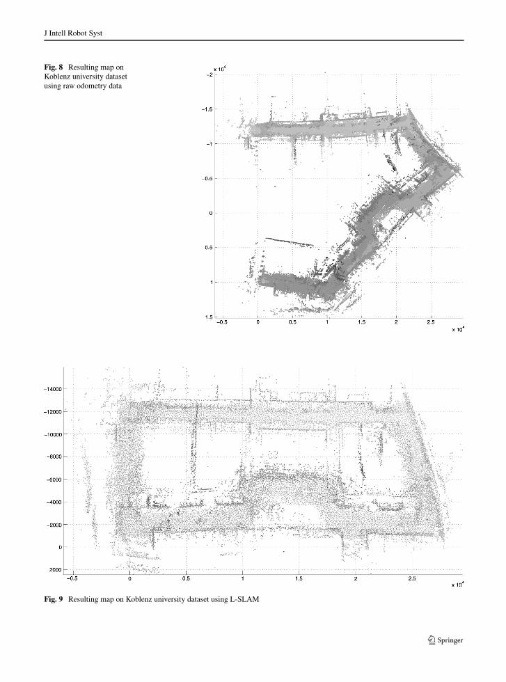
Fig. 9 Resulting map on Koblenz university dataset using L-SLAM

J Intell Robot Syst
(b) L-SLAM map(a) Raw odometry mapping
Fig. 10 Resulting map on Koblenz university dataset
5.2.2 University of Koblenz 3D Dataset
In this experiment the data acquired from the Uni-versity of Koblenz (Figs. 8, 9, 10). The data set wasrecorded using a Velodyne HDL-64E S2 3D laser sen-sor attached in a car which be driven at the UniversityCampus of Koblenz. The car covered a distance ofabout 700 meters in a closed loop. All the experimentrun with 5, 40 and 100 particles using L-SLAM andFastSLAM 1.0 and 2.0.
The comparison of the three methods made in thebasis of the mean execution time per step, the consis-tency that the algorithm presents and the resamplingrate. The consistency was measured as successful ornot in the case of the algorithm was able to close theloop efficiently while the resampling rate gives a mea-sure of the algorithm degeneration. All algorithms runfor 20 times in the same machine.
The results from this dataset (Table 6) showsclearly that the L-SLAM algorithm presents higherconsistency and is faster than the other two algo-rithms. It is noteworthy that in comparison with theFastSLAM 2.0 method the L-SLAM is almost threetimes faster while it presents almost the same or bet-ter results. Also the FastSLAM 1.0 algorithm exhibitszero consistency with few particles as a result of thehigh dimensionality of the problem.
6 Conclusions
In this paper we have presented the L-SLAM algo-rithm with unknown data association and comparedit with the FastSLAM 1.0 and 2.0 algorithms in theplanar problem as well as in the three dimensionalspace. In the planar problem the Car Park and the
Table 6 Comparisonresults among theFastSLAM 1.0, 2.0 andL-SLAM on the Koblenzdataset with loop closing.The vehicle moved once ina loop covering a distanceof about 700 meters
Algorithm Particles No Time (sec) Consistency % Resampling %
FastSLAM 1.0 5 2.3 0 % 97 %
FastSLAM 2.0 5 6.4 10 % 24 %
L-SLAM 5 1.7 20 % 69 %
FastSLAM 1.0 40 18.5 5 % 58 %
FastSLAM 2.0 40 58.9 85 % 9 %
L-SLAM 40 19.1 95 % 14 %
FastSLAM 1.0 100 42.3 30 % 60 %
FastSLAM 2.0 100 101.4 90 % 11 %
L-SLAM 100 39.2 90 % 13 %

J Intell Robot Syst
Victoria park datasets have used, while in the threedimensional space a simulated environment and theKoblenz dataset has been used. Comparison with theFastSLAM 1.0 and 2.0 methods in the simulated envi-ronment on three sets of experiments as well in thereal case scenarios has shown that FastSLAM 1.0 and2.0 were slower than L-SLAM due to the computa-tional complexity of the EKF. As expected, L-SLAMachieved more accurate results for a small number ofparticles than FastSLAM 1.0 and 2.0 due to the dimen-sionality reduction of the particle filter. For a largenumber of particles L-SLAM exhibits the same accu-racy as FastSLAM 2.0 but the time per step in the caseof L-SLAM is roughly one third of the one required inthe case of FastSLAM 2.0.
Appendix
Proof The SLAM posterior of Eq. 9 can be factor-ized into three posteriors for the particles filter, theKalman filter and the Kalman smoothing proceduresubsequently.
f (pt , ϕt , �|zt , ut , nt ) =f (ϕt |zt , ut , nt )︸ ︷︷ ︸
Particle filter
f (pt , θnt |ϕt , zt , ut , nt )︸ ︷︷ ︸Kalman filter
f (pt−1, �nt |pt , θnt , ϕt , zt , ut , nt )︸ ︷︷ ︸
Kalman smoothing
(45)
where
�nt = {θi |i = 1..M|i �= nt }The second posterior of the right side of Eq. 45 is
expanded as:
f (pt , θnt |ϕt , zt , ut , nt ) ∝f (zt |pt , θnt , ϕ
t , zt−1, ut , nt )f (pt , θnt |ϕt , zt−1, ut , nt ) (46)
which is translated to the known Kalman form of thepredict-update using iteratively the previous estima-tion as shown in Eq. 47
f (pt , θnt |ϕt , zt , ut , nt ) ∝ f (zt |pt , θnt , ϕt , zt−1, ut , nt )∫
f (pt , θtnt|pt−1, θ
t−1nt
, ϕt , zt−1, ut , nt )
f (pt−1, θt−1nt
|ϕt−1, zt−1, ut−1, nt−1)dpt−1, θt−1nt
(47)
The third posterior of the right side of Eq. 45 esti-mates the time series of the robot’s position up to timet − 1 and the unobserved features using the obser-vations and the inputs up to time t . This posterior isfactorized in Eq. 48.
f (pt−1, �nt |pt , θnt , ϕt , zt , ut , nt )
=0∏
i=t−1
f (pi, θni |pi:t , θni:t , ϕt , zt , ut , nt ) (48)
Each factor describes the smoothed instance of therobot’s and feature’s position regarding all the futureobservations. The proof of the Kalman smoothingalgorithm can be found in [2, 15].
References
1. Augenstein, S., Rock, S.: Simultaneous estimation of tar-get pose and 3-d shape using the fastslam algorithm. In:Proceedings of AIAA GNC 2009 (2009)
2. Briers, M., Doucet, A., Maskell, S.: Smoothing algorithmsfor state–space models. Ann. Inst. Stat. Math. 62(1), 61–89(2010). doi:10.1007/s10463-009-0236-2
3. Dissanayake, M., Newman, P., Clark, S., Durrant-Whyte,H., Csorba, M.: A solution to the simultaneous localiza-tion and map building (slam) problem. IEEE Trans. Robot.Autom. 17(3), 229–241 (2001)
4. Doucet, A., de Freitas, N., Murphy, K.P., Russell, S.J.:Rao-blackwellised particle filtering for dynamic Bayesiannetworks. In: UAI, pp. 176–183 (2000)
5. Kwak, N., Kim, G.W., Lee, B.H.: A new compensa-tion technique based on analysis of resampling pro-cess in fastslam. Robotica 26(2), 205–217 (2008).doi:10.1017/S0263574707003773
6. Montemerlo, M., Thrun, S.: Simultaneous localization andmapping with unknown data association using fastslam. In:Proceedings of IEEE International Conference on Roboticsand Automation, ICRA ’03, vol. 2, pp. 1985–1991 (2003).doi:10.1109/ROBOT.2003.1241885
7. Montemerlo, M., Thrun, S., Koller, D., Wegbreit, B.: Fast-SLAM: A factored solution to the simultaneous localizationand mapping problem. In: AAAI/IAAI, pp. 593–598 (2002)
8. Montemerlo, M., Thrun, S., Koller, D., Wegbreit, B.: Fast-SLAM 2.0: An improved particle filtering algorithm forsimultaneous localization and mapping that provably con-verges. In: IJCAI, pp. 1151–1156 (2003)
9. Montemerlo, M., Thrun, S., Siciliano, B.: FastSLAM: AScalable Method for the Simultaneous Localization andMapping Problem in Robotics, vol. 27. Springer, Berlin(2007)
10. Mullane, J., Vo, B.N., Adams, M., Vo, B.T.: A random finiteset approach to bayesian slam. In: IEEE trans. robotics, vol.27, pp. 268–282 (2011)
11. Mullane, J., Vo, B.N., Adams, M., Vo, B.T.: Random FiniteSets for Robotic Mapping and Slam: Tracts in AdvancedRobotics. Springer (2011)

J Intell Robot Syst
12. Nieto, J., Guivant, J., Nebot, E., Thrun, S.: Real time dataassociation for fastslam. In: Proceedings of IEEE Interna-tional Conference on Robotics and Automation, ICRA ’03,vol. 1, pp. 412–418 (2003)
13. Nuchter, A.: 3D robotic mapping: the simultaneous local-ization and mapping problem with six degrees of freedom.In: STAR: Springer tracts in advanced robotics, vol. 52.Springer (2009). http://www.loc.gov/catdir/enhancements/fy1102/2008941001-d.html
14. Petridis, V., Zikos, N.: L-slam: reduced dimensionality fast-slam algorithms. In: WCCI, pp. 2510–2516, Barcelona(2010)
15. Rauch, H.E., Striebel, C.T., Tung, F.: Maximum likelihoodestimates of linear dynamic systems. J. Am. Inst. Aeronaut.Astronaut. 3(8), 1445–1450 (1965)
16. Sarkka, S., Vehtari, A., Lampinen, J.: Time series predictionby kalman smoother with cross validated noise density. In:IJCNN, pp. 1653–1658. (2004) doi:10.1.1.76.9307
17. Sarkka, S., Vehtari, A., Lampinen, J.: Cats benchmark timeseries prediction by kalman smoother with cross- vali-
dated noise density. Neurocomputer 70(13–15), 2331–2341(2007). doi:10.1016/j.neucom.2005.12.132
18. Sasiadek, J., Monjazeb, A., Necsulescu, D.: Navigationof an autonomous mobile robot using ekf-slam and fast-slam. In: 2008 16th Mediterranean conference on Controland automation, pp. 517–522. (2008) doi:10.1109/MED.2008.4602213
19. Smith, R., Cheeseman, P.: On the representation and esti-mation of spatial uncertainty. Int. J. Robot. Res. 5(4), 56–68(1986)
20. Smith, R., Self, M., Cheeseman, P.: A stochastic map foruncertain spatial relationships. In: Proceedings of the 4thInternational Symposium on Robotics Research, pp. 467–474. MIT Press, Cambridge (1988)
21. Thrun, S., Montemerlo, M., Koller, D., Wegbreit, B., Nieto,J., Nebot, E.: Fastslam: An efficient solution to the simul-taneous localization and mapping problem with unknowndata association. J. Mach. Learn. Res. (2004)
22. Zikos, N., Petridis, V.: L-slam: reduced dimensionality fast-slam with unknown data association. In: ICRA, pp. 4074–4079. Shanghai (2011)