Embed Size (px)
Citation preview
5-AGWA-8
Crop evapotranspiration - Guidelines for computing crop water requirements - FAO Irrigation and drainage paper 56
Table of Contents
by Richard G. Allen Utah State University Logan, Utah, USA Luis S. Pereira Instituto Superior de Agronomia Lisbon, Portugal
Dirk Raes Katholieke Universiteit Leuven Leuven, Belgium Martin Smith Water Resources, Development and Management Service FAO FAO - Food and Agriculture Organization of the United Nations Rome, 1998
The designations employed and the presentation of material in this publication do not imply the expression of any opinion whatsoever on the part of the Food and Agriculture Organization of the United Nations concerning the legal status of any country, territory, city or area or of its authorities, or concerning the delimitation of its frontiers or boundaries.
M-56 ISBN 92-5-104219-5 All rights reserved. No part of this publication may be reproduced, stored in a retrieval system, or transmitted in any form or by any means, electronic, mechanical, photocopying or otherwise. without the prior permission of the copyright owner. Applications for such permission, with a statement of the purpose and extent of the reproduction, should be addressed to the Director, Information Division, Food and Agriculture Organization of the United Nations, Viale delle Terme di Caracalla, 00100 Rome, Italy. © FAO 1998 This electronic document has been scanned using optical character recognition (OCR) software and careful manual recorrection. Even if the quality of digitalisation is high, the FAO declines all responsibility for any discrepancies that may exist between the present document and its original printed version.
Table of Contents
Preface Acknowledgements List of principal symbols and acronyms Chapter 1 - Introduction to evapotranspiration
Evapotranspiration process
Evaporation Transpiration Evapotranspiration (ET)
Units Factors affecting evapotranspiration
Weather parameters Crop factors Management and environmental conditions
Evapotranspiration concepts
Reference crop evapotranspiration (ETo) Crop evapotranspiration under standard conditions (ETc) Crop evapotranspiration under non-standard conditions (ETc adj)
Determining evapotranspiration
ET measurement ET computed from meteorological data ET estimated from pan evaporation
Part A - Reference evapotranspiration (ETo)
Chapter 2 - FAO Penman-Monteith equation
Need for a standard ETo method Formulation of the Penman-Monteith equation
Penman-Monteith equation Aerodynamic resistance (ra)
(Bulk) surface resistance (rs)
Reference surface FAO Penman-Monteith equation
Equation Data Missing climatic data
Chapter 3 - Meteorological data
Meteorological factors determining ET
Solar radiation Air temperature Air humidity Wind speed
Atmospheric parameters
Atmospheric pressure (P) Latent heat of vaporization (λ) Psychrometric constant (γ)
Air temperature Air humidity
Concepts Measurement Calculation procedures
Radiation
Concepts Units Measurement Calculation procedures
Wind speed
Measurement Wind profile relationship
Climatic data acquisition
Weather stations Agroclimatic monthly databases
Estimating missing climatic data
Estimating missing humidity data Estimating missing radiation data Missing wind speed data
Minimum data requirements
An alternative equation for ETo when weather data are missing
Chapter 4 - Determination of ETo
Penman-Monteith equation
Calculation procedure ETo calculated with different time steps
Calculation procedures with missing data Pan evaporation method
Pan evaporation Pan coefficient (Kp)
Part B - Crop evapotranspiration under standard conditions
Chapter 5 - Introduction to crop evapotranspiration (ETc)
Calculation procedures
Direct calculation Crop coefficient approach
Factors determining the crop coefficient
Crop type Climate Soil evaporation Crop growth stages
Crop evapotranspiration (ETc)
Single and dual crop coefficient approaches Crop coefficient curve
Flow chart of the calculations
Chapter 6 - ETc - Single crop coefficient (Kc)
Length of growth stages Crop coefficients
Tabulated Kc values Crop coefficient for the initial stage (Kc ini) Crop coefficient for the mid-season stage (Kc
mid) Crop coefficient for the end of the late season stage (Kc end)
Construction of the Kc curve
Annual crops Kc curves for forage crops Fruit trees
Calculating ETc
Graphical determination of Kc Numerical determination of Kc
Alfalfa-based crop coefficients Transferability of previous Kc values
Chapter 7 - ETc - Dual crop coefficient (Kc = Kcb + Ke)
Transpiration component (Kcb ETo)
Basal crop coefficient (Kcb) Determination of daily Kcb values
Evaporation component (Ke ETo)
Calculation procedure Upper limit Kc max Soil evaporation reduction coefficient (Kr) Exposed and wetted soil fraction (few) Daily calculation of Ke
Calculating ETc
Part C - Crop evapotranspiration under non-standard conditions
Chapter 8 - ETc under soil water stress conditions
Soil water availability
Total available water (TAW) Readily available water (RAW)
Water stress coefficient (Ks) Soil water balance Forecasting or allocating irrigations Effects of soil salinity Yield-salinity relationship Yield-moisture stress relationship
Combined salinity-ET reduction relationship
No water stress (Dr < RAW) With water stress (Dr > RAW)
Application
Chapter 9 - ETc for natural, non-typical and non-pristine vegetation
Calculation approach
Initial growth stage Mid and late season stages Water stress conditions
Mid-season stage - Adjustment for sparse vegetation
Adjustment from simple field observations Estimation of Kcb
mid from Leaf Area Index (LAI) Estimation of Kcb
mid from effective ground cover (fc
eff) Estimation of Kcb
full Conclusion
Mid-season stage - Adjustment for stomatal control Late season stage Estimating ETc adj using crop yields
Chapter 10 - ETc under various management practices
Effects of surface mulches
Plastic mulches Organic mulches
Intercropping
Contiguous vegetation Overlapping vegetation Border crops
Small areas of vegetation
Areas surrounded by vegetation having similar roughness and moisture conditions Clothesline and oasis effects
Management induced environmental stress
Alfalfa seed Cotton Sugar beets Coffee Tea Olives
Chapter 11 - ETc during non-growing periods
Types of surface conditions
Bare soil Surface covered with dead vegetation Surface covered with live vegetation Frozen or snow covered surfaces
Annex 1. Units and symbols Annex 2. Meteorological tables Annex 3. Background on physical parameters used in evapotranspiration computations Annex 4. Statistical analysis of weather data sets Annex 5. Measuring and assessing integrity of weather data Annex 6. Correction of weather data observed in non-reference weather sites to compute ETo Annex 7. Background and computations for Kc for the initial stage for annual crops
Annex 8. Calculation example for applying the dual Kc procedure in irrigation scheduling Bibliography
A. Basic concepts and definitions B. ET equations C. ET and weather measurement D. Parameters in ET equations E. Crop parameters in PM equation F. Analysis of weather and ET data G. Crop evapotranspiration H. Crop coefficients I. Lengths of crop growth stages J. Effects of soil mulches K. Non-growing season evapotranspiration L. Soil water holding characteristics M. Rooting depths N. Salinity impacts on evapotranspiration O. Soil evaporation P. Factors affecting ETc Q. Soil water balance and irrigation scheduling R. General
FAO technical papers
Chapter 6 - ETc - Single crop coefficient (Kc)
Length of growth stages Crop coefficients Construction of the Kc curve Calculating ETc Alfalfa-based crop coefficients Transferability of previous Kc values
This chapter deals with the calculation of crop evapotranspiration (ETc) under standard conditions. No limitations are placed on crop growth or evapotranspiration from soil water and salinity stress, crop density, pests and diseases, weed infestation or low fertility. ETc is determined by the crop coefficient approach whereby the effect of the various weather conditions are incorporated into ETo and the crop characteristics into the Kc coefficient:
ETc = Kc ETo (58)
The effect of both crop transpiration and soil evaporation are integrated into a single crop coefficient. The Kc coefficient incorporates crop characteristics and averaged effects of evaporation from the soil. For normal irrigation planning and
management purposes, for the development of basic irrigation schedules, and for most hydrologic water balance studies, average crop coefficients are relevant and more convenient than the Kc computed on a daily time step using a separate crop and soil coefficient (Chapter 7). Only when values for Kc are needed on a daily basis for specific fields of crops and for specific years, must a separate transpiration and evaporation coefficient (Kcb + Ke) be considered. The calculation procedure for crop evapotranspiration, ETc, consists of:
1. identifying the crop growth stages, determining their lengths, and selecting the corresponding Kc coefficients;
2. adjusting the selected Kc coefficients for frequency of wetting or climatic conditions during the stage;
3. constructing the crop coefficient curve (allowing one to determine Kc values for any period during the growing period); and
4. calculating ETc as the product of ETo and Kc.
Length of growth stages
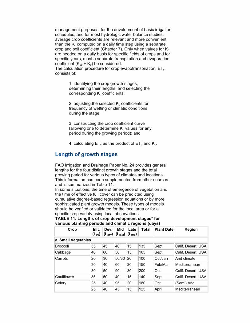
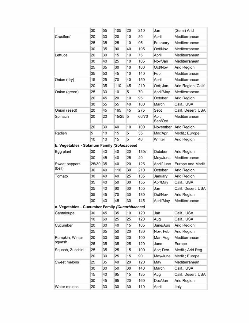
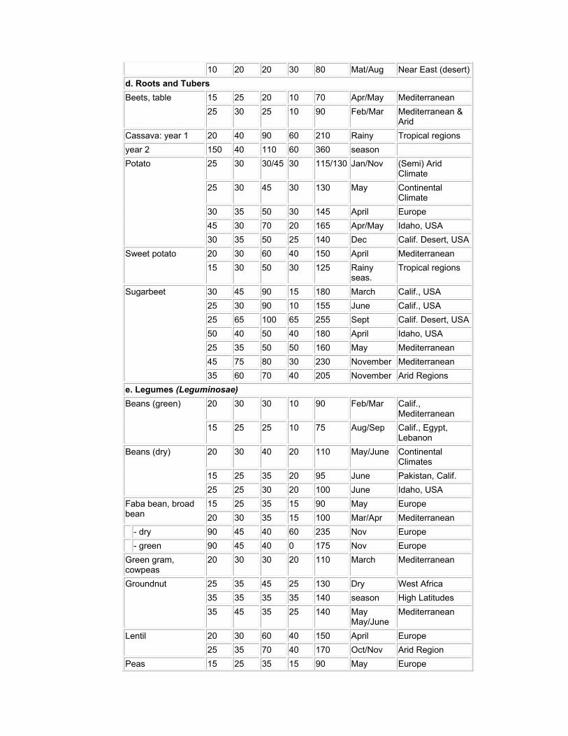
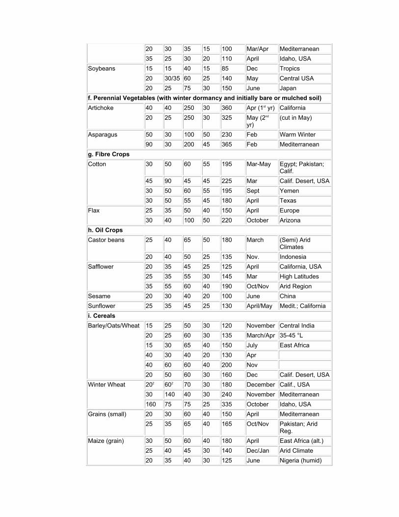
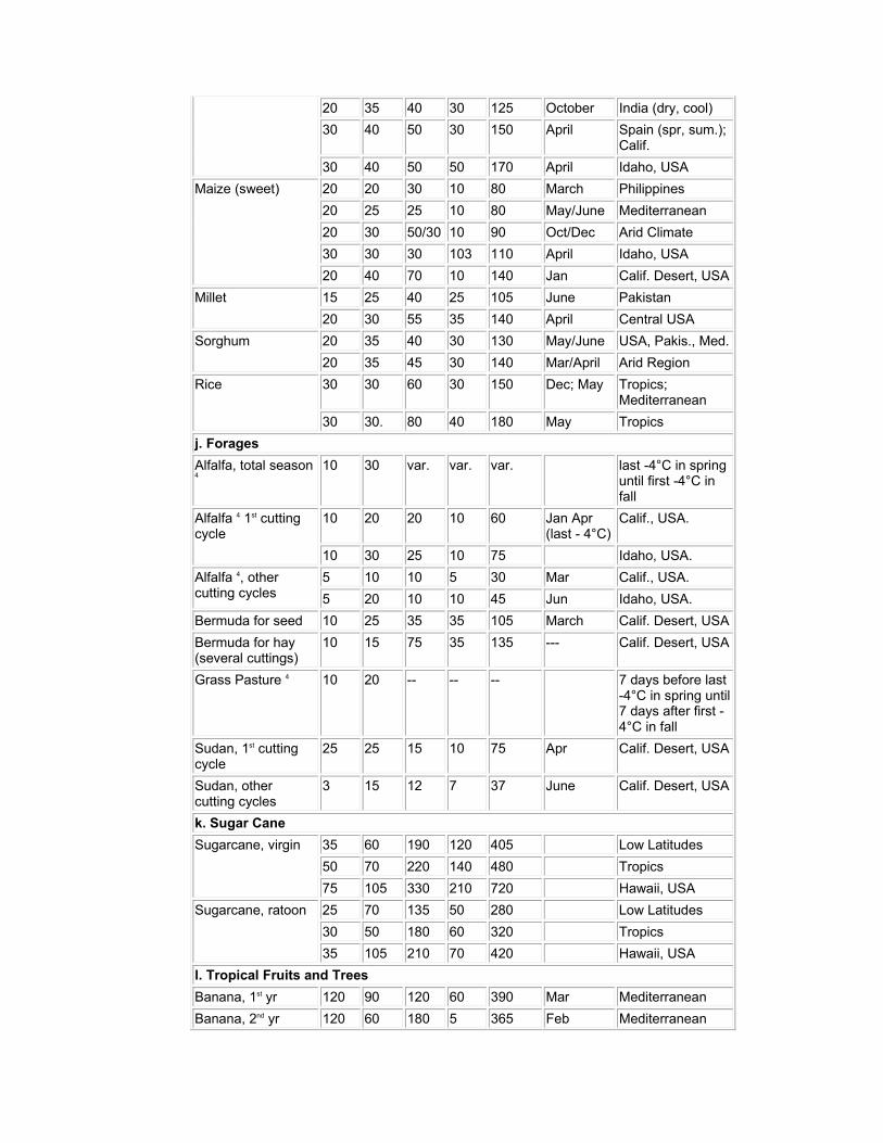
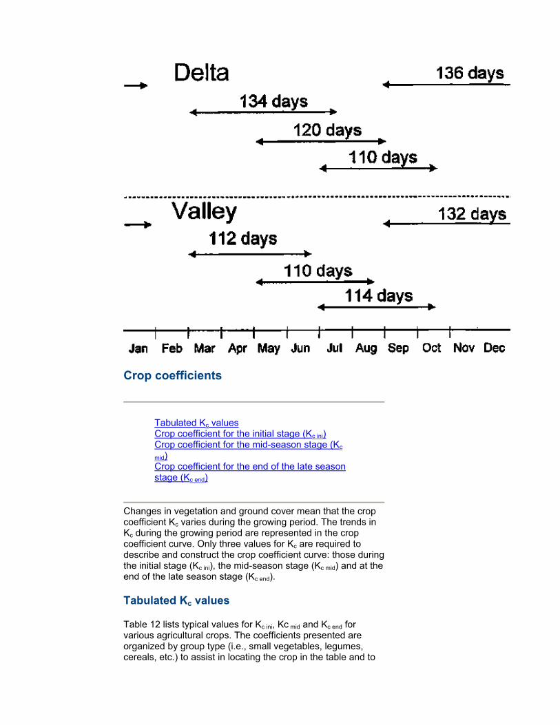
FAO Irrigation and Drainage Paper No. 24 provides general lengths for the four distinct growth stages and the total growing period for various types of climates and locations. This information has been supplemented from other sources and is summarized in Table 11. In some situations, the time of emergence of vegetation and the time of effective full cover can be predicted using cumulative degree-based regression equations or by more sophisticated plant growth models. These types of models should be verified or validated for the local area or for a specific crop variety using local observations. TABLE 11. Lengths of crop development stages* for various planting periods and climatic regions (days)
Crop Init. (Lini)
Dev. (Ldev)
Mid (Lmid)
Late (Llate)
Total Plant Date Region
a. Small Vegetables
Broccoli 35 45 40 15 135 Sept Calif. Desert, USA
Cabbage 40 60 50 15 165 Sept Calif. Desert, USA
Carrots 20 30 50/30 20 100 Oct/Jan Arid climate
30 40 60 20 150 Feb/Mar Mediterranean
30 50 90 30 200 Oct Calif. Desert, USA
Cauliflower 35 50 40 15 140 Sept Calif. Desert, USA
Celery 25 40 95 20 180 Oct (Semi) Arid
25 40 45 15 125 April Mediterranean
30 55 105 20 210 Jan (Semi) Arid
Crucifers1 20 30 20 10 80 April Mediterranean
25 35 25 10 95 February Mediterranean
30 35 90 40 195 Oct/Nov Mediterranean
Lettuce 20 30 15 10 75 April Mediterranean
30 40 25 10 105 Nov/Jan Mediterranean
25 35 30 10 100 Oct/Nov Arid Region
35 50 45 10 140 Feb Mediterranean
Onion (dry) 15 25 70 40 150 April Mediterranean
20 35 110 45 210 Oct; Jan. Arid Region; Calif.
Onion (green) 25 30 10 5 70 April/May Mediterranean
20 45 20 10 95 October Arid Region
30 55 55 40 180 March Calif., USA
Onion (seed) 20 45 165 45 275 Sept Calif. Desert, USA
Spinach 20 20 15/25 5 60/70 Apr; Sep/Oct
Mediterranean
20 30 40 10 100 November Arid Region
Radish 5 10 15 5 35 Mar/Apr Medit.; Europe
10 10 15 5 40 Winter Arid Region
b. Vegetables - Solanum Family (Solanaceae)
Egg plant 30 40 40 20 130\1 October Arid Region
30 45 40 25 40 May/June Mediterranean
Sweet peppers (bell)
25/30 35 40 20 125 April/June Europe and Medit.
30 40 110 30 210 October Arid Region
Tomato 30 40 40 25 135 January Arid Region
35 40 50 30 155 Apr/May Calif., USA
25 40 60 30 155 Jan Calif. Desert, USA
35 45 70 30 180 Oct/Nov Arid Region
30 40 45 30 145 April/May Mediterranean
c. Vegetables - Cucumber Family (Cucurbitaceae)
Cantaloupe 30 45 35 10 120 Jan Calif., USA
10 60 25 25 120 Aug Calif., USA
Cucumber 20 30 40 15 105 June/Aug Arid Region
25 35 50 20 130 Nov; Feb Arid Region
Pumpkin, Winter squash
20 30 30 20 100 Mar, Aug Mediterranean
25 35 35 25 120 June Europe
Squash, Zucchini 25 35 25 15 100 Apr; Dec. Medit.; Arid Reg.
20 30 25 15 90 May/June Medit.; Europe
Sweet melons 25 35 40 20 120 May Mediterranean
30 30 50 30 140 March Calif., USA
15 40 65 15 135 Aug Calif. Desert, USA
30 45 65 20 160 Dec/Jan Arid Region
Water melons 20 30 30 30 110 April Italy
10 20 20 30 80 Mat/Aug Near East (desert)
d. Roots and Tubers
Beets, table 15 25 20 10 70 Apr/May Mediterranean
25 30 25 10 90 Feb/Mar Mediterranean & Arid
Cassava: year 1 20 40 90 60 210 Rainy Tropical regions
year 2 150 40 110 60 360 season
Potato 25 30 30/45 30 115/130 Jan/Nov (Semi) Arid Climate
25 30 45 30 130 May Continental Climate
30 35 50 30 145 April Europe
45 30 70 20 165 Apr/May Idaho, USA
30 35 50 25 140 Dec Calif. Desert, USA
Sweet potato 20 30 60 40 150 April Mediterranean
15 30 50 30 125 Rainy seas.
Tropical regions
Sugarbeet 30 45 90 15 180 March Calif., USA
25 30 90 10 155 June Calif., USA
25 65 100 65 255 Sept Calif. Desert, USA
50 40 50 40 180 April Idaho, USA
25 35 50 50 160 May Mediterranean
45 75 80 30 230 November Mediterranean
35 60 70 40 205 November Arid Regions
e. Legumes (Leguminosae)
Beans (green) 20 30 30 10 90 Feb/Mar Calif., Mediterranean
15 25 25 10 75 Aug/Sep Calif., Egypt, Lebanon
Beans (dry) 20 30 40 20 110 May/June Continental Climates
15 25 35 20 95 June Pakistan, Calif.
25 25 30 20 100 June Idaho, USA
Faba bean, broad bean
15 25 35 15 90 May Europe
20 30 35 15 100 Mar/Apr Mediterranean
- dry 90 45 40 60 235 Nov Europe
- green 90 45 40 0 175 Nov Europe
Green gram, cowpeas
20 30 30 20 110 March Mediterranean
Groundnut 25 35 45 25 130 Dry West Africa
35 35 35 35 140 season High Latitudes
35 45 35 25 140 May May/June
Mediterranean
Lentil 20 30 60 40 150 April Europe
25 35 70 40 170 Oct/Nov Arid Region
Peas 15 25 35 15 90 May Europe
20 30 35 15 100 Mar/Apr Mediterranean
35 25 30 20 110 April Idaho, USA
Soybeans 15 15 40 15 85 Dec Tropics
20 30/35 60 25 140 May Central USA
20 25 75 30 150 June Japan
f. Perennial Vegetables (with winter dormancy and initially bare or mulched soil)
Artichoke 40 40 250 30 360 Apr (1st yr) California
20 25 250 30 325 May (2nd yr)
(cut in May)
Asparagus 50 30 100 50 230 Feb Warm Winter
90 30 200 45 365 Feb Mediterranean
g. Fibre Crops
Cotton 30 50 60 55 195 Mar-May Egypt; Pakistan; Calif.
45 90 45 45 225 Mar Calif. Desert, USA
30 50 60 55 195 Sept Yemen
30 50 55 45 180 April Texas
Flax 25 35 50 40 150 April Europe
30 40 100 50 220 October Arizona
h. Oil Crops
Castor beans 25 40 65 50 180 March (Semi) Arid Climates
20 40 50 25 135 Nov. Indonesia
Safflower 20 35 45 25 125 April California, USA
25 35 55 30 145 Mar High Latitudes
35 55 60 40 190 Oct/Nov Arid Region
Sesame 20 30 40 20 100 June China
Sunflower 25 35 45 25 130 April/May Medit.; California
i. Cereals
Barley/Oats/Wheat 15 25 50 30 120 November Central India
20 25 60 30 135 March/Apr 35-45 °L
15 30 65 40 150 July East Africa
40 30 40 20 130 Apr
40 60 60 40 200 Nov
20 50 60 30 160 Dec Calif. Desert, USA
Winter Wheat 202 602 70 30 180 December Calif., USA
30 140 40 30 240 November Mediterranean
160 75 75 25 335 October Idaho, USA
Grains (small) 20 30 60 40 150 April Mediterranean
25 35 65 40 165 Oct/Nov Pakistan; Arid Reg.
Maize (grain) 30 50 60 40 180 April East Africa (alt.)
25 40 45 30 140 Dec/Jan Arid Climate
20 35 40 30 125 June Nigeria (humid)
20 35 40 30 125 October India (dry, cool)
30 40 50 30 150 April Spain (spr, sum.); Calif.
30 40 50 50 170 April Idaho, USA
Maize (sweet) 20 20 30 10 80 March Philippines
20 25 25 10 80 May/June Mediterranean
20 30 50/30 10 90 Oct/Dec Arid Climate
30 30 30 103 110 April Idaho, USA
20 40 70 10 140 Jan Calif. Desert, USA
Millet 15 25 40 25 105 June Pakistan
20 30 55 35 140 April Central USA
Sorghum 20 35 40 30 130 May/June USA, Pakis., Med.
20 35 45 30 140 Mar/April Arid Region
Rice 30 30 60 30 150 Dec; May Tropics; Mediterranean
30 30. 80 40 180 May Tropics
j. Forages
Alfalfa, total season 4
10 30 var. var. var. last -4°C in spring until first -4°C in fall
Alfalfa 4 1st cutting cycle
10 20 20 10 60 Jan Apr (last - 4°C)
Calif., USA.
10 30 25 10 75 Idaho, USA.
Alfalfa 4, other cutting cycles
5 10 10 5 30 Mar Calif., USA.
5 20 10 10 45 Jun Idaho, USA.
Bermuda for seed 10 25 35 35 105 March Calif. Desert, USA
Bermuda for hay (several cuttings)
10 15 75 35 135 --- Calif. Desert, USA
Grass Pasture 4 10 20 -- -- -- 7 days before last -4°C in spring until 7 days after first -4°C in fall
Sudan, 1st cutting cycle
25 25 15 10 75 Apr Calif. Desert, USA
Sudan, other cutting cycles
3 15 12 7 37 June Calif. Desert, USA
k. Sugar Cane
Sugarcane, virgin 35 60 190 120 405 Low Latitudes
50 70 220 140 480 Tropics
75 105 330 210 720 Hawaii, USA
Sugarcane, ratoon 25 70 135 50 280 Low Latitudes
30 50 180 60 320 Tropics
35 105 210 70 420 Hawaii, USA
l. Tropical Fruits and Trees
Banana, 1st yr 120 90 120 60 390 Mar Mediterranean
Banana, 2nd yr 120 60 180 5 365 Feb Mediterranean
Pineapple 60 120 600 10 790 Hawaii, USA
m. Grapes and Berries
Grapes 20 40 120 60 240 April Low Latitudes
20 50 75 60 205 Mar Calif., USA
20 50 90 20 180 May High Latitudes
30 60 40 80 210 April Mid Latitudes (wine)
Hops 25 40 80 10 155 April Idaho, USA
n. Fruit Trees
Citrus 60 90 120 95 365 Jan Mediterranean
Deciduous Orchard 20 70 90 30 210 March High Latitudes
20 70 120 60 270 March Low Latitudes
30 50 130 30 240 March Calif., USA
Olives 30 90 60 90 2705 March Mediterranean
Pistachios 20 60 30 40 150 Feb Mediterranean
Walnuts 20 10 130 30 190 April Utah, USA
o. Wetlands - Temperate Climate
Wetlands (Cattails, Bulrush)
10 30 80 20 140 May Utah, USA; killing frost
180 60 90 35 365 November Florida, USA
Wetlands (short veg.)
180 60 90 35 365 November frost-free climate
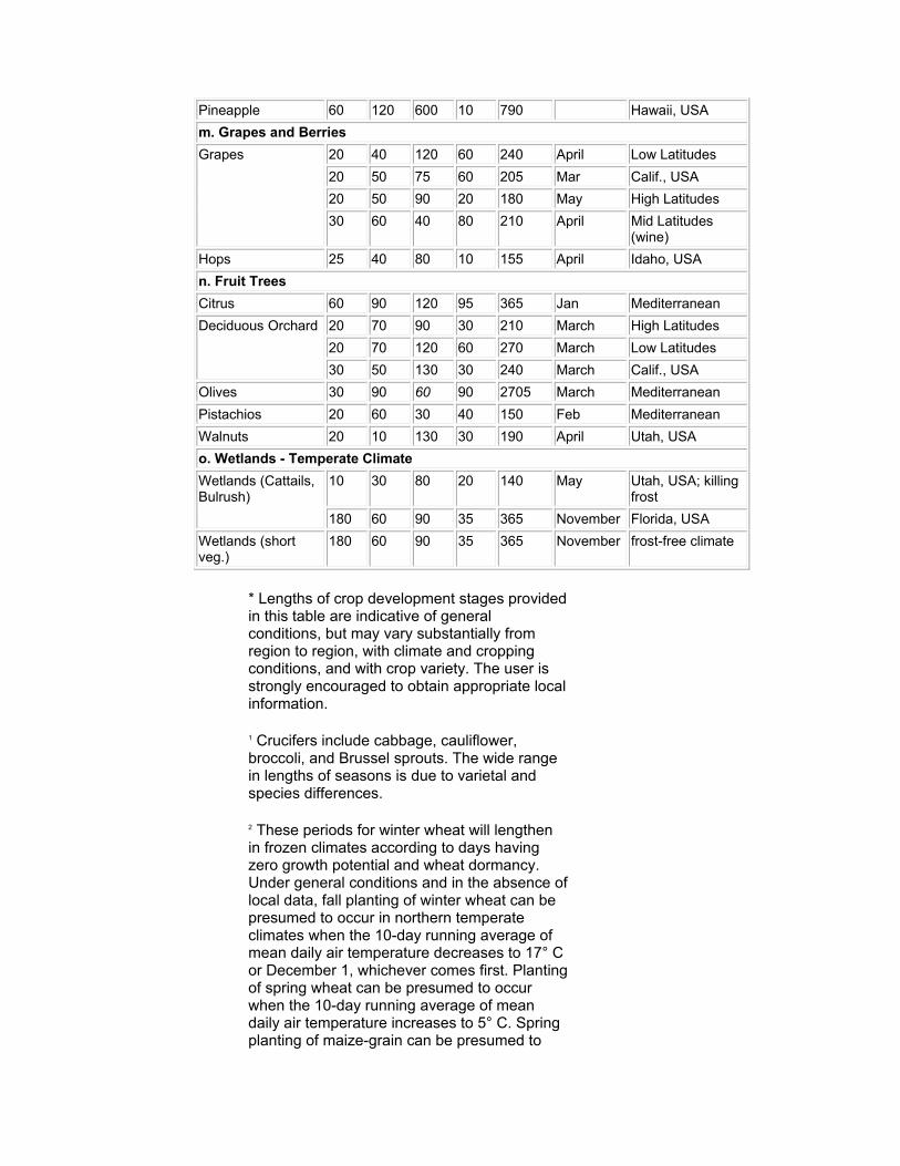
* Lengths of crop development stages provided in this table are indicative of general conditions, but may vary substantially from region to region, with climate and cropping conditions, and with crop variety. The user is strongly encouraged to obtain appropriate local information.
1 Crucifers include cabbage, cauliflower, broccoli, and Brussel sprouts. The wide range in lengths of seasons is due to varietal and species differences.
2 These periods for winter wheat will lengthen in frozen climates according to days having zero growth potential and wheat dormancy. Under general conditions and in the absence of local data, fall planting of winter wheat can be presumed to occur in northern temperate climates when the 10-day running average of mean daily air temperature decreases to 17° C or December 1, whichever comes first. Planting of spring wheat can be presumed to occur when the 10-day running average of mean daily air temperature increases to 5° C. Spring planting of maize-grain can be presumed to
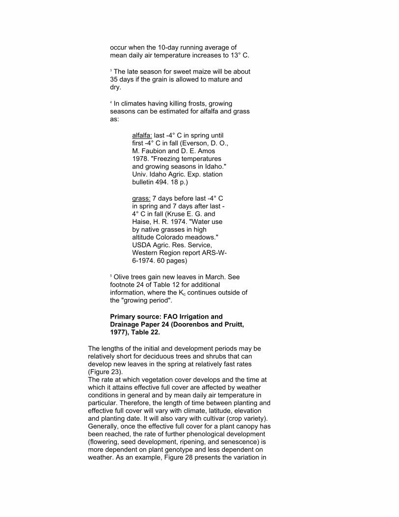
occur when the 10-day running average of mean daily air temperature increases to 13° C.
3 The late season for sweet maize will be about 35 days if the grain is allowed to mature and dry.
4 In climates having killing frosts, growing seasons can be estimated for alfalfa and grass as:
alfalfa: last -4° C in spring until first -4° C in fall (Everson, D. O., M. Faubion and D. E. Amos 1978. "Freezing temperatures and growing seasons in Idaho." Univ. Idaho Agric. Exp. station bulletin 494. 18 p.)
grass: 7 days before last -4° C in spring and 7 days after last -4° C in fall (Kruse E. G. and Haise, H. R. 1974. "Water use by native grasses in high altitude Colorado meadows." USDA Agric. Res. Service, Western Region report ARS-W-6-1974. 60 pages)
5 Olive trees gain new leaves in March. See footnote 24 of Table 12 for additional information, where the Kc continues outside of the "growing period".
Primary source: FAO Irrigation and Drainage Paper 24 (Doorenbos and Pruitt, 1977), Table 22.
The lengths of the initial and development periods may be relatively short for deciduous trees and shrubs that can develop new leaves in the spring at relatively fast rates (Figure 23). The rate at which vegetation cover develops and the time at which it attains effective full cover are affected by weather conditions in general and by mean daily air temperature in particular. Therefore, the length of time between planting and effective full cover will vary with climate, latitude, elevation and planting date. It will also vary with cultivar (crop variety). Generally, once the effective full cover for a plant canopy has been reached, the rate of further phenological development (flowering, seed development, ripening, and senescence) is more dependent on plant genotype and less dependent on weather. As an example, Figure 28 presents the variation in

length of the growing period for one cultivar of rice for one region and for various planting dates. The end of the mid-season and beginning of the late season is usually marked by senescence of leaves, often beginning with the lower leaves of plants. The length of the late season period may be relatively short (less than 10 days) for vegetation killed by frost (for example, maize at high elevations in latitudes > 40°N) or for agricultural crops that are harvested fresh (for example, table beets and small vegetables). High temperatures may accelerate the ripening and senescence of crops. Long duration of high air temperature (> 35°C) can cause some crops such as turf grass to go into dormancy. If severely high air temperatures are coupled with moisture stress, the dormancy of grass can be permanent for the remainder of the growing season. Moisture stress or other environmental stresses will usually accelerate the rate of crop maturation and can shorten the mid and late season growing periods. The values in Table 11 are useful only as a general guide and for comparison purposes. The listed lengths of growth stages are average lengths for the regions and periods specified and are intended to serve only as examples. Local observations of the specific plant stage development should be used, wherever possible, to incorporate effects of plant variety, climate and cultural practices. Local information can be obtained by interviewing farmers, ranchers, agricultural extension agents and local researchers, by conducting local surveys, or by remote sensing. When determining stage dates from local observations, the guidelines and visual descriptions may be helpful. FIGURE 28. Variation in the length of the growing period
of rice (cultivar: Jaya) sown during various months of the year at different locations along the Senegal River
(Africa)
Crop coefficients
Tabulated Kc values Crop coefficient for the initial stage (Kc ini) Crop coefficient for the mid-season stage (Kc
mid) Crop coefficient for the end of the late season stage (Kc end)
Changes in vegetation and ground cover mean that the crop coefficient Kc varies during the growing period. The trends in Kc during the growing period are represented in the crop coefficient curve. Only three values for Kc are required to describe and construct the crop coefficient curve: those during the initial stage (Kc ini), the mid-season stage (Kc mid) and at the end of the late season stage (Kc end).
Tabulated Kc values
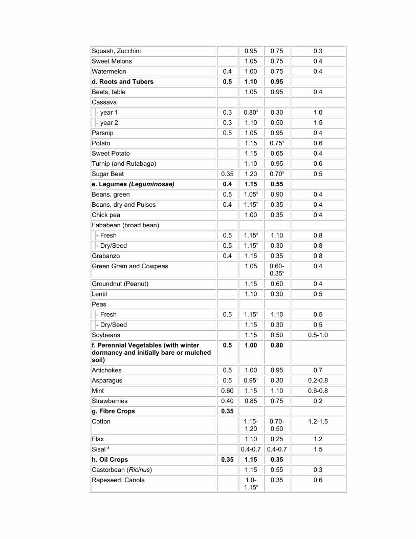
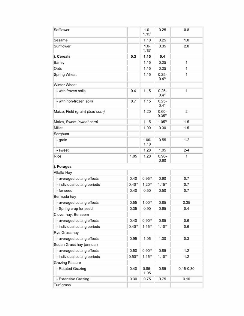
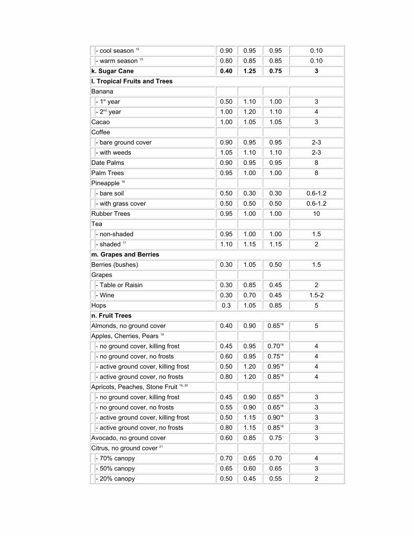
Table 12 lists typical values for Kc ini, Kc mid and Kc end for various agricultural crops. The coefficients presented are organized by group type (i.e., small vegetables, legumes, cereals, etc.) to assist in locating the crop in the table and to
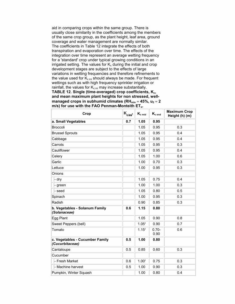
aid in comparing crops within the same group. There is usually close similarity in the coefficients among the members of the same crop group, as the plant height, leaf area, ground coverage and water management are normally similar. The coefficients in Table 12 integrate the effects of both transpiration and evaporation over time. The effects of the integration over time represent an average wetting frequency for a 'standard' crop under typical growing conditions in an irrigated setting. The values for Kc during the initial and crop development stages are subject to the effects of large variations in wetting frequencies and therefore refinements to the value used for Kc ini should always be made. For frequent wettings such as with high frequency sprinkler irrigation or rainfall, the values for Kc ini may increase substantially. TABLE 12. Single (time-averaged) crop coefficients, Kc, and mean maximum plant heights for non stressed, well-managed crops in subhumid climates (RHmin ≈ 45%, u2 ≈ 2 m/s) for use with the FAO Penman-Monteith ETo.
Crop Kc mid Kc end Maximum Crop Height (h) (m)
a. Small Vegetables 0.7 1.05 0.95
Broccoli 1.05 0.95 0.3
Brussel Sprouts 1.05 0.95 0.4
Cabbage 1.05 0.95 0.4
Carrots 1.05 0.95 0.3
Cauliflower 1.05 0.95 0.4
Celery 1.05 1.00 0.6
Garlic 1.00 0.70 0.3
Lettuce 1.00 0.95 0.3
Onions
- dry 1.05 0.75 0.4
- green 1.00 1.00 0.3
- seed 1.05 0.80 0.5
Spinach 1.00 0.95 0.3
Radish 0.90 0.85 0.3
b. Vegetables - Solanum Family (Solanaceae)
0.6 1.15 0.80
Egg Plant 1.05 0.90 0.8
Sweet Peppers (bell) 1.052 0.90 0.7
Tomato 1.152 0.70-0.90
0.6
c. Vegetables - Cucumber Family (Cucurbitaceae)
0.5 1.00 0.80
Cantaloupe 0.5 0.85 0.60 0.3
Cucumber
- Fresh Market 0.6 1.002 0.75 0.3
- Machine harvest 0.5 1.00 0.90 0.3
Pumpkin, Winter Squash 1.00 0.80 0.4
Squash, Zucchini 0.95 0.75 0.3
Sweet Melons 1.05 0.75 0.4
Watermelon 0.4 1.00 0.75 0.4
d. Roots and Tubers 0.5 1.10 0.95
Beets, table 1.05 0.95 0.4
Cassava
- year 1 0.3 0.803 0.30 1.0
- year 2 0.3 1.10 0.50 1.5
Parsnip 0.5 1.05 0.95 0.4
Potato 1.15 0.754 0.6
Sweet Potato 1.15 0.65 0.4
Turnip (and Rutabaga) 1.10 0.95 0.6
Sugar Beet 0.35 1.20 0.705 0.5
e. Legumes (Leguminosae) 0.4 1.15 0.55
Beans, green 0.5 1.052 0.90 0.4
Beans, dry and Pulses 0.4 1.152 0.35 0.4
Chick pea 1.00 0.35 0.4
Fababean (broad bean)
- Fresh 0.5 1.152 1.10 0.8
- Dry/Seed 0.5 1.152 0.30 0.8
Grabanzo 0.4 1.15 0.35 0.8
Green Gram and Cowpeas 1.05 0.60-0.356
0.4
Groundnut (Peanut) 1.15 0.60 0.4
Lentil 1.10 0.30 0.5
Peas
- Fresh 0.5 1.152 1.10 0.5
- Dry/Seed 1.15 0.30 0.5
Soybeans 1.15 0.50 0.5-1.0
f. Perennial Vegetables (with winter dormancy and initially bare or mulched soil)
0.5 1.00 0.80
Artichokes 0.5 1.00 0.95 0.7
Asparagus 0.5 0.957 0.30 0.2-0.8
Mint 0.60 1.15 1.10 0.6-0.8
Strawberries 0.40 0.85 0.75 0.2
g. Fibre Crops 0.35
Cotton 1.15-1.20
0.70-0.50
1.2-1.5
Flax 1.10 0.25 1.2
Sisal 8 0.4-0.7 0.4-0.7 1.5
h. Oil Crops 0.35 1.15 0.35
Castorbean (Ricinus) 1.15 0.55 0.3
Rapeseed, Canola 1.0-1.159
0.35 0.6
Safflower 1.0-1.159
0.25 0.8
Sesame 1.10 0.25 1.0
Sunflower 1.0-1.159
0.35 2.0
i. Cereals 0.3 1.15 0.4
Barley 1.15 0.25 1
Oats 1.15 0.25 1
Spring Wheat 1.15 0.25-0.410
1
Winter Wheat
- with frozen soils 0.4 1.15 0.25-0.410
1
- with non-frozen soils 0.7 1.15 0.25-0.410
Maize, Field (grain) (field corn) 1.20 0.60-0.3511
2
Maize, Sweet (sweet corn) 1.15 1.0512 1.5
Millet 1.00 0.30 1.5
Sorghum
- grain 1.00-1.10
0.55 1-2
- sweet 1.20 1.05 2-4
Rice 1.05 1.20 0.90-0.60
1
j. Forages
Alfalfa Hay
- averaged cutting effects 0.40 0.9513 0.90 0.7
- individual cutting periods 0.4014 1.2014 1.1514 0.7
- for seed 0.40 0.50 0.50 0.7
Bermuda hay
- averaged cutting effects 0.55 1.0013 0.85 0.35
- Spring crop for seed 0.35 0.90 0.65 0.4
Clover hay, Berseem
- averaged cutting effects 0.40 0.9013 0.85 0.6
- individual cutting periods 0.4014 1.1514 1.1014 0.6
Rye Grass hay
- averaged cutting effects 0.95 1.05 1.00 0.3
Sudan Grass hay (annual)
- averaged cutting effects 0.50 0.9014 0.85 1.2
- individual cutting periods 0.5014 1.1514 1.1014 1.2
Grazing Pasture
- Rotated Grazing 0.40 0.85-1.05
0.85 0.15-0.30
- Extensive Grazing 0.30 0.75 0.75 0.10
Turf grass
- cool season 15 0.90 0.95 0.95 0.10
- warm season 15 0.80 0.85 0.85 0.10
k. Sugar Cane 0.40 1.25 0.75 3
l. Tropical Fruits and Trees
Banana
- 1st year 0.50 1.10 1.00 3
- 2nd year 1.00 1.20 1.10 4
Cacao 1.00 1.05 1.05 3
Coffee
- bare ground cover 0.90 0.95 0.95 2-3
- with weeds 1.05 1.10 1.10 2-3
Date Palms 0.90 0.95 0.95 8
Palm Trees 0.95 1.00 1.00 8
Pineapple 16
- bare soil 0.50 0.30 0.30 0.6-1.2
- with grass cover 0.50 0.50 0.50 0.6-1.2
Rubber Trees 0.95 1.00 1.00 10
Tea
- non-shaded 0.95 1.00 1.00 1.5
- shaded 17 1.10 1.15 1.15 2
m. Grapes and Berries
Berries (bushes) 0.30 1.05 0.50 1.5
Grapes
- Table or Raisin 0.30 0.85 0.45 2
- Wine 0.30 0.70 0.45 1.5-2
Hops 0.3 1.05 0.85 5
n. Fruit Trees
Almonds, no ground cover 0.40 0.90 0.6518 5
Apples, Cherries, Pears 19
- no ground cover, killing frost 0.45 0.95 0.7018 4
- no ground cover, no frosts 0.60 0.95 0.7518 4
- active ground cover, killing frost 0.50 1.20 0.9518 4
- active ground cover, no frosts 0.80 1.20 0.8518 4
Apricots, Peaches, Stone Fruit 19, 20
- no ground cover, killing frost 0.45 0.90 0.6518 3
- no ground cover, no frosts 0.55 0.90 0.6518 3
- active ground cover, killing frost 0.50 1.15 0.9018 3
- active ground cover, no frosts 0.80 1.15 0.8518 3
Avocado, no ground cover 0.60 0.85 0.75 3
Citrus, no ground cover 21
- 70% canopy 0.70 0.65 0.70 4
- 50% canopy 0.65 0.60 0.65 3
- 20% canopy 0.50 0.45 0.55 2
Citrus, with active ground cover or weeds 22
- 70% canopy 0.75 0.70 0.75 4
- 50% canopy 0.80 0.80 0.80 3
- 20% canopy 0.85 0.85 0.85 2
Conifer Trees 23 1.00 1.00 1.00 10
Kiwi 0.40 1.05 1.05 3
Olives (40 to 60% ground coverage by canopy) 24
0.65 0.70 0.70 3-5
Pistachios, no ground cover 0.40 1.10 0.45 3-5
Walnut Orchard 19 0.50 1.10 0.6518 4-5
o. Wetlands - temperate climate
Cattails, Bulrushes, killing frost 0.30 1.20 0.30 2
Cattails, Bulrushes, no frost 0.60 1.20 0.60 2
Short Veg., no frost 1.05 1.10 1.10 0.3
Reed Swamp, standing water 1.00 1.20 1.00 1-3
Reed Swamp, moist soil 0.90 1.20 0.70 1-3
p. Special
Open Water, < 2 m depth or in subhumid climates or tropics
1.05 1.05
Open Water, > 5 m depth, clear of turbidity, temperate climate
0.6525 1.2525
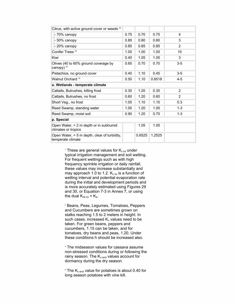
1 These are general values for Kc ini under typical irrigation management and soil wetting. For frequent wettings such as with high frequency sprinkle irrigation or daily rainfall, these values may increase substantially and may approach 1.0 to 1.2. Kc ini is a function of wetting interval and potential evaporation rate during the initial and development periods and is more accurately estimated using Figures 29 and 30, or Equation 7-3 in Annex 7, or using the dual Kcb ini + Ke.
2 Beans, Peas, Legumes, Tomatoes, Peppers and Cucumbers are sometimes grown on stalks reaching 1.5 to 2 meters in height. In such cases, increased Kc values need to be taken. For green beans, peppers and cucumbers, 1.15 can be taken, and for tomatoes, dry beans and peas, 1.20. Under these conditions h should be increased also.
3 The midseason values for cassava assume non-stressed conditions during or following the rainy season. The Kc end values account for dormancy during the dry season.
4 The Kc end value for potatoes is about 0.40 for long season potatoes with vine kill.

5 This Kc end value is for no irrigation during the last month of the growing season. The Kc end value for sugar beets is higher, up to 1.0, when irrigation or significant rain occurs during the last month.
6 The first Kc end is for harvested fresh. The second value is for harvested dry.
7 The Kc for asparagus usually remains at Kc ini during harvest of the spears, due to sparse ground cover. The Kc mid value is for following regrowth of plant vegetation following termination of harvest of spears.
8 Kc for sisal depends on the planting density and water management (e.g., intentional moisture stress).
9 The lower values are for rainfed crops having less dense plant populations.
10 The higher value is for hand-harvested crops.
11 The first Kc end value is for harvest at high grain moisture. The second Kc end value is for harvest after complete field drying of the grain (to about 18% moisture, wet mass basis).
12 If harvested fresh for human consumption. Use Kc end for field maize if the sweet maize is allowed to mature and dry in the field.
13 This Kc mid coefficient for hay crops is an overall average Kc mid coefficient that averages Kc for both before and following cuttings. It is applied to the period following the first development period until the beginning of the last late season period of the growing season.
14 These Kc coefficients for hay crops represent immediately following cutting; at full cover; and immediately before cutting, respectively. The growing season is described as a series of individual cutting periods (Figure 35).
15 Cool season grass varieties include dense stands of bluegrass, ryegrass, and fescue. Warm season varieties include bermuda grass and St. Augustine grass. The 0.95 values for cool season grass represent a 0.06 to 0.08 m mowing height under general turf conditions. Where careful water management is practiced
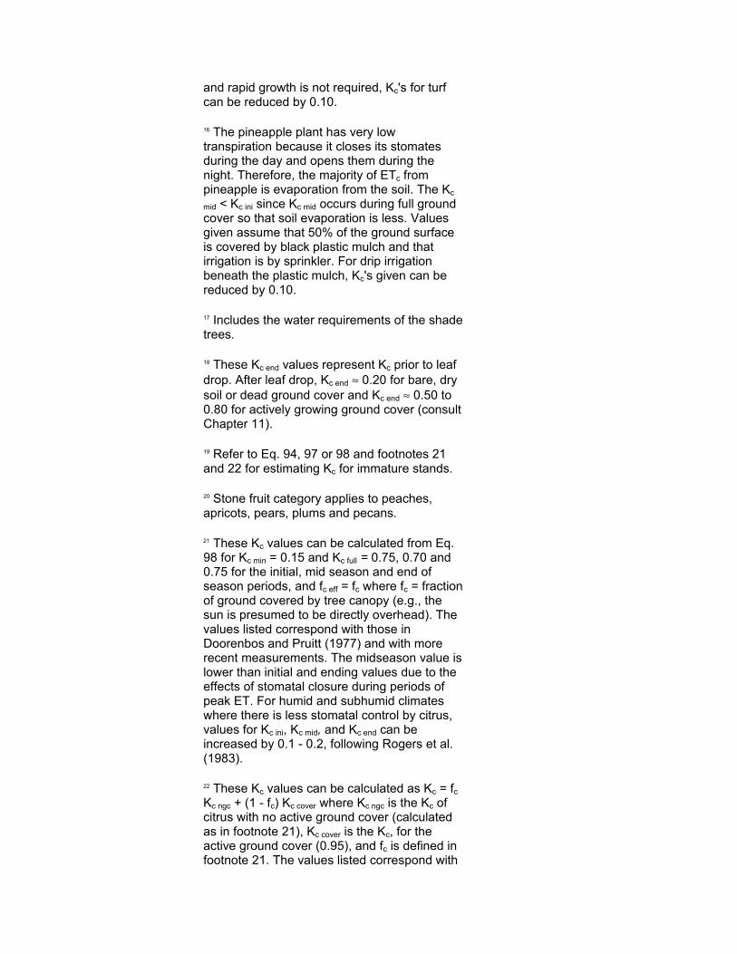
and rapid growth is not required, Kc's for turf can be reduced by 0.10.
16 The pineapple plant has very low transpiration because it closes its stomates during the day and opens them during the night. Therefore, the majority of ETc from pineapple is evaporation from the soil. The Kc
mid < Kc ini since Kc mid occurs during full ground cover so that soil evaporation is less. Values given assume that 50% of the ground surface is covered by black plastic mulch and that irrigation is by sprinkler. For drip irrigation beneath the plastic mulch, Kc's given can be reduced by 0.10.
17 Includes the water requirements of the shade trees.
18 These Kc end values represent Kc prior to leaf drop. After leaf drop, Kc end ≈ 0.20 for bare, dry soil or dead ground cover and Kc end ≈ 0.50 to 0.80 for actively growing ground cover (consult Chapter 11).
19 Refer to Eq. 94, 97 or 98 and footnotes 21 and 22 for estimating Kc for immature stands.
20 Stone fruit category applies to peaches, apricots, pears, plums and pecans.
21 These Kc values can be calculated from Eq. 98 for Kc min = 0.15 and Kc full = 0.75, 0.70 and 0.75 for the initial, mid season and end of season periods, and fc eff = fc where fc = fraction of ground covered by tree canopy (e.g., the sun is presumed to be directly overhead). The values listed correspond with those in Doorenbos and Pruitt (1977) and with more recent measurements. The midseason value is lower than initial and ending values due to the effects of stomatal closure during periods of peak ET. For humid and subhumid climates where there is less stomatal control by citrus, values for Kc ini, Kc mid, and Kc end can be increased by 0.1 - 0.2, following Rogers et al. (1983).
22 These Kc values can be calculated as Kc = fc Kc ngc + (1 - fc) Kc cover where Kc ngc is the Kc of citrus with no active ground cover (calculated as in footnote 21), Kc cover is the Kc, for the active ground cover (0.95), and fc is defined in footnote 21. The values listed correspond with
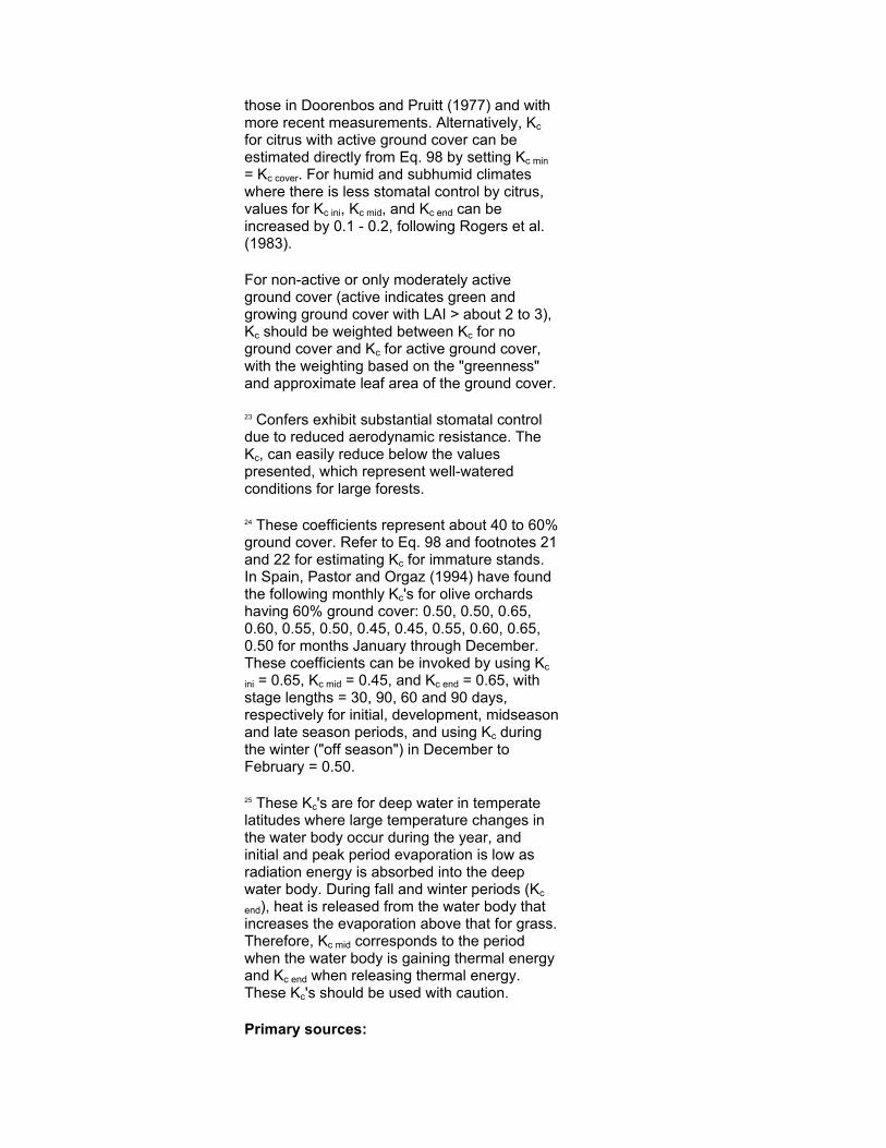
those in Doorenbos and Pruitt (1977) and with more recent measurements. Alternatively, Kc for citrus with active ground cover can be estimated directly from Eq. 98 by setting Kc min = Kc cover. For humid and subhumid climates where there is less stomatal control by citrus, values for Kc ini, Kc mid, and Kc end can be increased by 0.1 - 0.2, following Rogers et al. (1983).
For non-active or only moderately active ground cover (active indicates green and growing ground cover with LAI > about 2 to 3), Kc should be weighted between Kc for no ground cover and Kc for active ground cover, with the weighting based on the "greenness" and approximate leaf area of the ground cover.
23 Confers exhibit substantial stomatal control due to reduced aerodynamic resistance. The Kc, can easily reduce below the values presented, which represent well-watered conditions for large forests.
24 These coefficients represent about 40 to 60% ground cover. Refer to Eq. 98 and footnotes 21 and 22 for estimating Kc for immature stands. In Spain, Pastor and Orgaz (1994) have found the following monthly Kc's for olive orchards having 60% ground cover: 0.50, 0.50, 0.65, 0.60, 0.55, 0.50, 0.45, 0.45, 0.55, 0.60, 0.65, 0.50 for months January through December. These coefficients can be invoked by using Kc
ini = 0.65, Kc mid = 0.45, and Kc end = 0.65, with stage lengths = 30, 90, 60 and 90 days, respectively for initial, development, midseason and late season periods, and using Kc during the winter ("off season") in December to February = 0.50.
25 These Kc's are for deep water in temperate latitudes where large temperature changes in the water body occur during the year, and initial and peak period evaporation is low as radiation energy is absorbed into the deep water body. During fall and winter periods (Kc
end), heat is released from the water body that increases the evaporation above that for grass. Therefore, Kc mid corresponds to the period when the water body is gaining thermal energy and Kc end when releasing thermal energy. These Kc's should be used with caution.
Primary sources:
Kc ini: Doorenbos and Kassam (1979) Kc mid and Kc end: Doorenbos and Pruitt (1977); Pruitt (1986); Wright (1981, 1982). Snyder et al., (1989)
The values for Kc mid and Kc end in Table 12 represent those for a sub-humid climate with an average daytime minimum relative humidity (RHmin) of about 45% and with calm to moderate wind speeds averaging 2 m/s. For more humid or arid conditions, or for more or less windy conditions, the Kc coefficients for the mid-season and end of late season stage should be modified as described in this chapter. The values for Kc in Table 12 are values for non-stressed crops cultivated under excellent agronomic and water management conditions and achieving maximum crop yield (standard conditions). Where stand density, height or leaf area are less than that attained under such conditions, the value for Kc mid and, for most crops, for Kc end will need to be modified (Part C, Chapters 8, 9 and 10).
Crop coefficient for the initial stage (Kc ini)
Calculation procedure The values for Kc ini in Table 12 are only approximations and should only be used for estimating ETc during preliminary or planning studies. For several group types only one value for Kc ini is listed and it is considered to be representative of the whole group for a typical irrigation water management. More accurate estimates of Kc ini can be obtained by considering:
Time interval between wetting events
Evapotranspiration during the initial stage for annual crops is predominately in the form of evaporation. Therefore, accurate estimates for Kc ini should consider the frequency with which the soil surface is wetted during the initial period. Where the soil is frequently wet from irrigation or rain, the evaporation from the soil surface can be considerable and Kc ini will be large. On the other hand, where the soil surface is dry, evaporation is restricted and the Kc ini will be small (Table 9).
Evaporation power of the atmosphere
The value of Kc ini is affected by the evaporating power of the atmosphere, i.e., ETo. The higher the evaporation power of the atmosphere, the quicker the soil will dry between water applications and the smaller the time-averaged Kc will be for any particular period.
Magnitude of the wetting event
As the amount of water available in the topsoil for evaporation and hence the time for the soil surface to dry is a function of the magnitude of the wetting event, Kc ini will be smaller for light wetting events than for large wettings.
Depending on the time interval between wetting events, the magnitude of the wetting event, and the evaporation power of the atmosphere, Kc ini can vary between 0.1 and 1.15. A numerical procedure to compute Kc ini is provided in Annex 7. Time interval between wetting events In general, the mean time interval between wetting events is estimated by counting all rainfall and irrigation events occurring during the initial period that are greater than a few millimetres. Wetting events occurring on adjacent days can be counted as one event. The mean wetting interval is estimated by dividing the length of the initial period by the number of events. Where only monthly rainfall values are available without any information on the number of rainy days, the number of events within the month can be estimated by dividing the monthly rainfall depth by the depth of a typical rain event. The typical depth, if it exists, can vary widely from climate to climate, region to region and from season to season. Table 13 presents some information on the range of rainfall depths. After deciding what rainfall is typical for the region and time of the year, the number of rainy days and the mean wetting interval can be estimated. TABLE 13. Classification of rainfall depths
rain event depth
Very light (drizzle) ≤ 3 mm
Light (light showers) 5 mm
Medium (showers) ≥ 10 mm
Heavy (rainstorms) ≥ 40 mm
Where rainfall is insufficient, irrigation is needed to keep the crop well watered. Even where irrigation is not yet developed, the mean interval between the future irrigations should be estimated to obtain the required frequency of wetting
necessary to keep the crop stress free. The interval might be as small as a few days for small vegetables, but up to a week or longer for cereals depending on the climatic conditions. Where no estimate of the interval can be made, the user may refer to the values for Kc ini of Table 12. EXAMPLE 23. Estimation of interval between wetting events
Estimate, from mean monthly rainfall data, the interval between rains during the rainy season for a station in a temperate climate (Paris, France: 50 mm/month), dry climate (Gafsa, Tunisia: 20 mm/month) and tropical climate (Calcutta, India: 300 mm/month).
Station monthly rain (mm/month)
typical rainfall (mm)
number of rainy days
interval between rains
Paris 50 3 17 ~ 2 days
Gafsa 20 5 4 weekly
Calcutta 300 20 15 ~ 2 days
Determination of Kc ini The crop coefficient for the initial growth stage can be derived from Figures 29 and 30 which provide estimates for Kc ini as a function of the average interval between wetting events, the evaporation power ETo, and the importance of the wetting event. Light wetting events (infiltration depths of 10 mm or less): rainfall and high frequency irrigation systems Figure 29 is used for all soil types when wetting events are light. When wetting during the initial period is only by precipitation, one will usually use Figure 29 to determine Kc ini. The graph can also be used when irrigation is by high frequency systems such as microirrigation and centre pivot and light applications of about 10 mm or less per wetting event are applied. EXAMPLE 24. Graphical determination of Kc ini
A silt loam soil receives irrigation every two days during the initial growth stage via a centre pivot irrigation system. The average depth applied by the centre pivot system is about 12 mm per event and the average ETo during the initial stage is 4 mm/day. Estimate the crop evapotranspiration during that stage.
From Fig. 29 using the 2-day interval curve:
Kc ini = 0.85 -
ETc = Kc ETo = 0.85 (4.0) =
3.4 mm/day
The average crop evapotranspiration during the initial growth stage is 3.4 mm/day
Heavy wetting events (infiltration depths of 40 mm or more): surface and sprinkler irrigation Figure 30 is used for heavy wetting events when infiltration depths are greater than 40 mm, such as for when wetting is primarily by periodic irrigation such as by sprinkler or surface irrigation. Following a wetting event, the amount of water available in the topsoil for evaporation is considerable, and the time for the soil surface to dry might be significantly increased. Consequently, the average Kc factor is larger than for light wetting events. As the time for the soil surface to dry is, apart from the evaporation power and the frequency of wetting, also determined by the water storage capacity of the topsoil, a distinction is made between soil types.
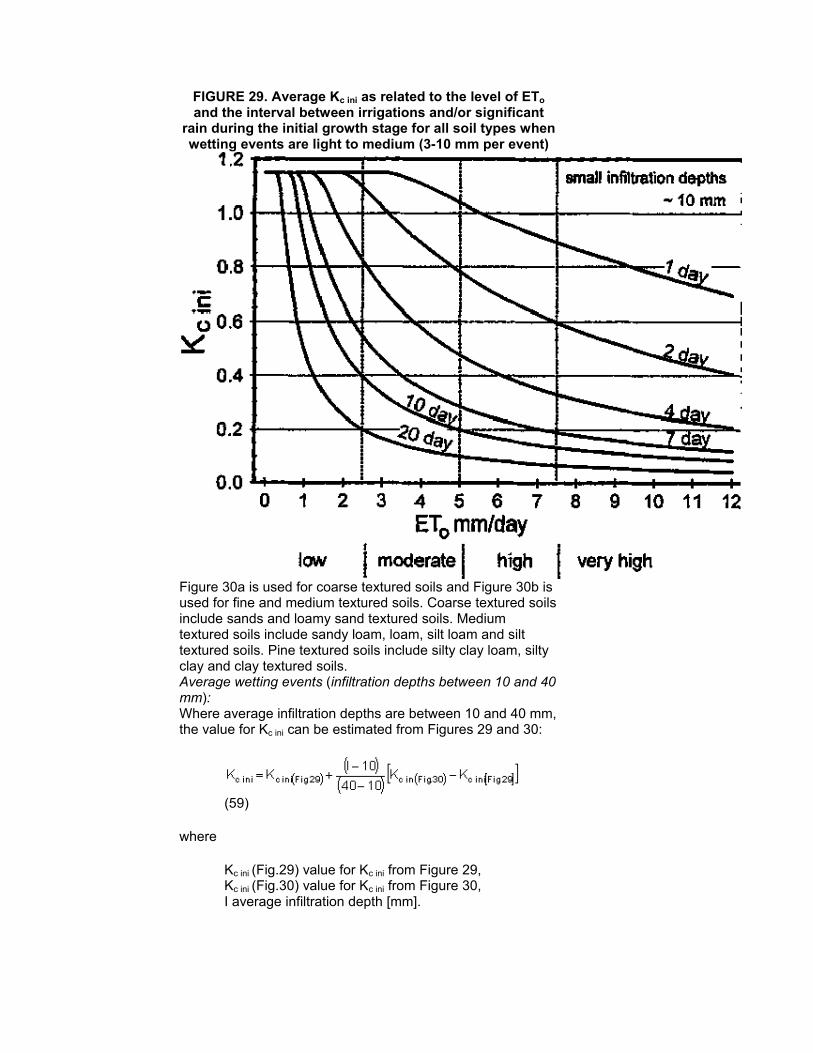
FIGURE 29. Average Kc ini as related to the level of ETo and the interval between irrigations and/or significant
rain during the initial growth stage for all soil types when wetting events are light to medium (3-10 mm per event)
Figure 30a is used for coarse textured soils and Figure 30b is used for fine and medium textured soils. Coarse textured soils include sands and loamy sand textured soils. Medium textured soils include sandy loam, loam, silt loam and silt textured soils. Pine textured soils include silty clay loam, silty clay and clay textured soils. Average wetting events (infiltration depths between 10 and 40 mm): Where average infiltration depths are between 10 and 40 mm, the value for Kc ini can be estimated from Figures 29 and 30:
(59)
where
Kc ini (Fig.29) value for Kc ini from Figure 29, Kc ini (Fig.30) value for Kc ini from Figure 30, I average infiltration depth [mm].
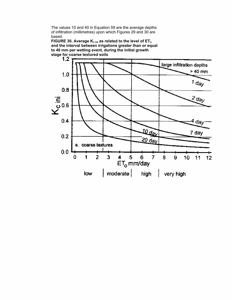
The values 10 and 40 in Equation 59 are the average depths of infiltration (millimetres) upon which Figures 29 and 30 are based. FIGURE 30. Average Kc ini as related to the level of ETo and the interval between irrigations greater than or equal to 40 mm per wetting event, during the initial growth stage for coarse textured soils
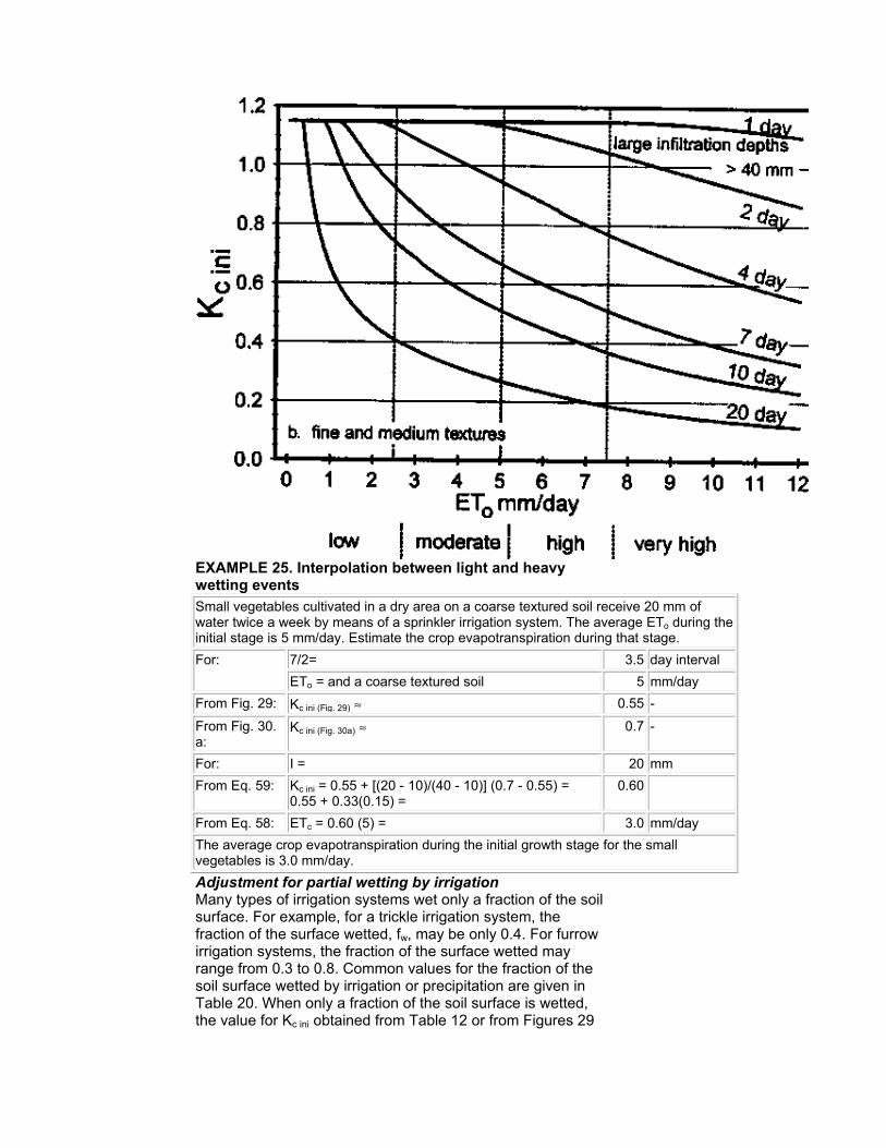
EXAMPLE 25. Interpolation between light and heavy wetting events
Small vegetables cultivated in a dry area on a coarse textured soil receive 20 mm of water twice a week by means of a sprinkler irrigation system. The average ETo during the initial stage is 5 mm/day. Estimate the crop evapotranspiration during that stage.
For: 7/2= 3.5 day interval
ETo = and a coarse textured soil 5 mm/day
From Fig. 29: Kc ini (Fig. 29) ≈ 0.55 -
From Fig. 30. a:
Kc ini (Fig. 30a) ≈ 0.7 -
For: I = 20 mm
From Eq. 59: Kc ini = 0.55 + [(20 - 10)/(40 - 10)] (0.7 - 0.55) = 0.55 + 0.33(0.15) =
0.60
From Eq. 58: ETc = 0.60 (5) = 3.0 mm/day
The average crop evapotranspiration during the initial growth stage for the small vegetables is 3.0 mm/day.
Adjustment for partial wetting by irrigation Many types of irrigation systems wet only a fraction of the soil surface. For example, for a trickle irrigation system, the fraction of the surface wetted, fw, may be only 0.4. For furrow irrigation systems, the fraction of the surface wetted may range from 0.3 to 0.8. Common values for the fraction of the soil surface wetted by irrigation or precipitation are given in Table 20. When only a fraction of the soil surface is wetted, the value for Kc ini obtained from Table 12 or from Figures 29
or 30 should be multiplied by the fraction of the surface wetted to adjust for the partial wetting:
Kc ini = fw Kc ini (Tab, Fig) (60)
where
fw the fraction of surfaced wetted by irrigation or rain [0 - 1], Kc ini (Tab Fig) the value for Kc ini from Table 12 or Figure 29 or 30.
In addition, in selecting which figure to use (i.e., Figure 29 or 30), the average infiltrated depth, expressed in millimetres over the entire field surface, should be divided by fw to represent the true infiltrated depth of water for the part of the surface that is wetted (Figure 31):
(61)
where
Iw irrigation depth for the part of the surface that is wetted [mm], fw fraction of surface wetted by irrigation, I the irrigation depth for the field [mm].
When irrigation of part of the soil surface and precipitation over the entire soil surface both occur during the initial period, fw should represent the average of fw for each type of wetting, weighted according to the total infiltration depth received by each type. FIGURE 31. Partial wetting by irrigation EXAMPLE 26. Determination of Kc ini for partial wetting of the soil surface
Determine the evapotranspiration of the crop in Example 24 if it had been irrigated using a trickle system every two days (with 12 mm each application expressed as an equivalent depth over the field area), and where the average fraction of surface wet was 0.4, and where little or no precipitation occurred during the initial period.
The average depth of infiltration per event in the wetted fraction of the surface:
From Eq. 61; lw = I/fw = 12 mm/0.4 = 30 mm
Therefore, one can interpolate between Fig. 29 representing light wetting events (~10 mm per event) and Fig. 30.b representing medium textured soil and large wetting events (~40 mm per event).
For: ETo = 4 mm/day 4 mm/day
and: a 2 day wetting interval: - -
Fig. 29 produces: Kc ini = 0.85 0.85 -
Fig. 30.b produces Kc ini = 1.15 1.15 -
From Eq. 59: Kc ini = 0.85 + [(30-10)/(40-10)] (1.15 - 0.85) = 1.05 -
Because the fraction of soil surface wetted by the trickle system is 0.4, the actual Kc ini for
the trickle irrigation is calculated as:
From Eq. 60: Kc ini = fw Kc ini Fig = 0.4 (1.05) = 0.42 -
This value (0.42) represents the Kc ini as applied over the entire field area.
- ETc =Kc ini ETo = 0.42(4) = 1.7 mm/day
The average crop evapotranspiration during the initial growth stage for this trickle irrigated crop is 1.7 mm/day.
Kc ini for trees and shrubs Kc ini for trees and shrubs should reflect the ground condition prior to leaf emergence or initiation in case of deciduous trees or shrubs, and the ground condition during the dormancy or low active period for evergreen trees and shrubs. The Kc ini depends upon the amount of grass or weed cover, frequency of soil wetting, tree density and mulch density. For a deciduous orchard in frost-free climates, the Kc ini can be as high as 0.8 or 0.9, where grass ground cover exists, and as low as 0.3 or 0.4 when the soil surface is kept bare and wetting is infrequent. The Kc ini for an evergreen orchard (having no concerted leaf drop) with a dormant period has less variation from Kc mid, as exemplified for citrus in Table 12, footnotes 21 and 22. For 50% canopy or less, the Kc ini also reflects ground cover conditions (bare soil, mulch or active grass or weed cover). Kc ini for paddy rice For rice growing in paddy fields with a water depth of 0.10-0.20 m, the ETc during the initial stage mainly consists of evaporation from the standing water. The Kc ini in Table 12 is 1.05 for a sub-humid climate with calm to moderate wind speeds. The Kc ini should be adjusted for the local climate as indicated in Table 14. TABLE 14. Kc ini for rice for various climatic conditions
Humidity Wind speed
light moderate strong
arid - semi-arid 1.10 1.15 1.20
sub-humid - humid 1.05 1.10 1.15
very humid 1.00 1.05 1.10
Crop coefficient for the mid-season stage (Kc mid)
Illustration of the climatic effect Typical values for the crop coefficient for the mid-season growth stage, Kc mid, are listed in Table 12 for various agricultural crops. As discussed in Chapter 5, the effect of the difference in aerodynamic properties between the grass reference surface and agricultural crops is not only crop specific but also varies with the climatic conditions and crop height (Figure 21). More arid climates and conditions of greater wind speed will have higher values for Kc mid. More humid climates and conditions of lower wind speed will have lower values for Kc mid. The relative impact of climate on Kc mid is illustrated in Figure 32 where the adjustments to the values from Table 12 are
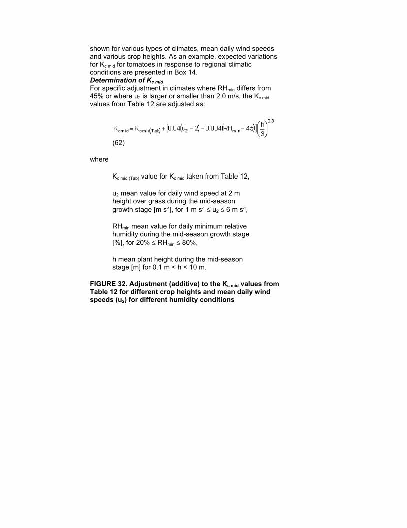
shown for various types of climates, mean daily wind speeds and various crop heights. As an example, expected variations for Kc mid for tomatoes in response to regional climatic conditions are presented in Box 14. Determination of Kc mid For specific adjustment in climates where RHmin differs from 45% or where u2 is larger or smaller than 2.0 m/s, the Kc mid values from Table 12 are adjusted as:
(62)
where
Kc mid (Tab) value for Kc mid taken from Table 12,
u2 mean value for daily wind speed at 2 m height over grass during the mid-season growth stage [m s-1], for 1 m s-1 ≤ u2 ≤ 6 m s-1,
RHmin mean value for daily minimum relative humidity during the mid-season growth stage [%], for 20% ≤ RHmin ≤ 80%,
h mean plant height during the mid-season stage [m] for 0.1 m < h < 10 m.
FIGURE 32. Adjustment (additive) to the Kc mid values from Table 12 for different crop heights and mean daily wind speeds (u2) for different humidity conditions

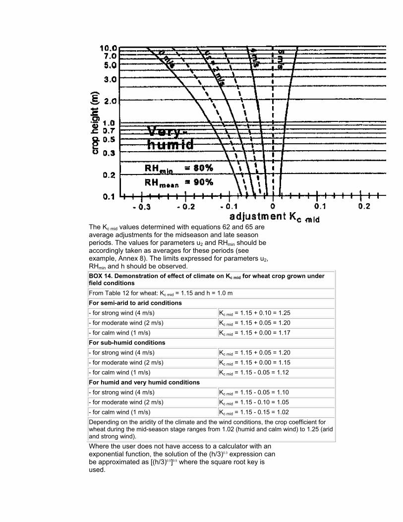
The Kc mid values determined with equations 62 and 65 are average adjustments for the midseason and late season periods. The values for parameters u2 and RHmin should be accordingly taken as averages for these periods (see example, Annex 8). The limits expressed for parameters u2, RHmin and h should be observed.
BOX 14. Demonstration of effect of climate on Kc mid for wheat crop grown under field conditions
From Table 12 for wheat: Kc mid = 1.15 and h = 1.0 m
For semi-arid to arid conditions
- for strong wind (4 m/s) Kc mid = 1.15 + 0.10 = 1.25
- for moderate wind (2 m/s) Kc mid = 1.15 + 0.05 = 1.20
- for calm wind (1 m/s) Kc mid = 1.15 + 0.00 = 1.17
For sub-humid conditions
- for strong wind (4 m/s) Kc mid = 1.15 + 0.05 = 1.20
- for moderate wind (2 m/s) Kc mid = 1.15 + 0.00 = 1.15
- for calm wind (1 m/s) Kc mid = 1.15 - 0.05 = 1.12
For humid and very humid conditions
- for strong wind (4 m/s) Kc mid = 1.15 - 0.05 = 1.10
- for moderate wind (2 m/s) Kc mid = 1.15 - 0.10 = 1.05
- for calm wind (1 m/s) Kc mid = 1.15 - 0.15 = 1.02
Depending on the aridity of the climate and the wind conditions, the crop coefficient for wheat during the mid-season stage ranges from 1.02 (humid and calm wind) to 1.25 (arid and strong wind).
Where the user does not have access to a calculator with an exponential function, the solution of the (h/3)0.3 expression can be approximated as [(h/3)0.5]0.5 where the square root key is used.

RHmin is used rather than RHmean because it is easier to approximate RHmin from Tmax where relative humidity data are unavailable. Moreover, under the common condition where Tmin approaches Tdew (i.e., RHmax ≈ 100%), the vapour pressure deficit (es - ea), with es from Equation 12 and ea from Equation 17, becomes [(100 - RHmin)/200] e°(Tmax), where e°(Tmax) is saturation vapour pressure at maximum daily air temperature. This indicates that RHmin better reflects the impact of vapour pressure deficit on Kc than does RHmean. RHmin is calculated on a daily or average monthly basis as:
(63)
where Tdew is mean dewpoint temperature and Tmax is mean daily maximum air temperature during the mid-season growth stage. Where dewpoint temperature or other hygrométrie data are not available or are of questionable quality, RHmin can be estimated by substituting mean daily minimum air temperature, Tmin, for Tdew
1. Then:
(64)
1 In the case of arid and semi-arid climates, Tmin in equation (64) should be adjusted as indicated in Annex 6 (equation 6-6) by subtracting 2°C from the average value of Tmin to better approximate Tdew.
The values for u2 and RHmin need only be approximate for the mid-season growth stage. This is because Equation 62 is not strongly sensitive to these values, changing 0.04 per 1 m/s change in u2 and per 10% change in RHmin for a 3 m tall crop. Measurements, calculation, and estimation of missing wind and humidity data are provided in Chapter 3. Wind speed measured at other than 2 m height should be adjusted to reflect values for wind speed at 2 m over grass using Equation 47. Where no data on u2 or RHmin are available, the general classification for wind speed and humidity data given in Tables 15 and 16 can be used. TABLE 15. Empirical estimates of monthly wind speed data
description mean monthly wind speed at 2 m
light wind ...≤ 1.0 m/s
light to moderate wind 2.0 m/s
moderate to strong wind 4.0 m/s
strong wind ... ≥ 5.0 m/s
general global conditions 2 m/s
TABLE 16. Typical values for RHmin compared with RHmean for general climatic classifications
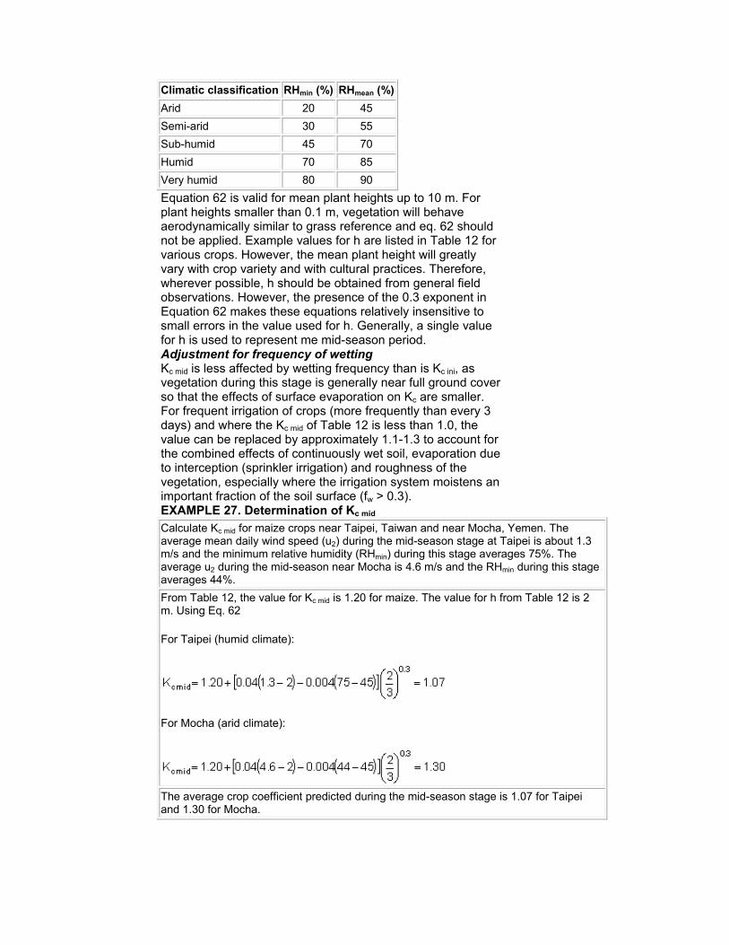
Climatic classification RHmin (%) RHmean (%)
Arid 20 45
Semi-arid 30 55
Sub-humid 45 70
Humid 70 85
Very humid 80 90
Equation 62 is valid for mean plant heights up to 10 m. For plant heights smaller than 0.1 m, vegetation will behave aerodynamically similar to grass reference and eq. 62 should not be applied. Example values for h are listed in Table 12 for various crops. However, the mean plant height will greatly vary with crop variety and with cultural practices. Therefore, wherever possible, h should be obtained from general field observations. However, the presence of the 0.3 exponent in Equation 62 makes these equations relatively insensitive to small errors in the value used for h. Generally, a single value for h is used to represent me mid-season period. Adjustment for frequency of wetting Kc mid is less affected by wetting frequency than is Kc ini, as vegetation during this stage is generally near full ground cover so that the effects of surface evaporation on Kc are smaller. For frequent irrigation of crops (more frequently than every 3 days) and where the Kc mid of Table 12 is less than 1.0, the value can be replaced by approximately 1.1-1.3 to account for the combined effects of continuously wet soil, evaporation due to interception (sprinkler irrigation) and roughness of the vegetation, especially where the irrigation system moistens an important fraction of the soil surface (fw > 0.3). EXAMPLE 27. Determination of Kc mid
Calculate Kc mid for maize crops near Taipei, Taiwan and near Mocha, Yemen. The average mean daily wind speed (u2) during the mid-season stage at Taipei is about 1.3 m/s and the minimum relative humidity (RHmin) during this stage averages 75%. The average u2 during the mid-season near Mocha is 4.6 m/s and the RHmin during this stage averages 44%.
From Table 12, the value for Kc mid is 1.20 for maize. The value for h from Table 12 is 2 m. Using Eq. 62
For Taipei (humid climate):
For Mocha (arid climate):
The average crop coefficient predicted during the mid-season stage is 1.07 for Taipei and 1.30 for Mocha.
Crop coefficient for the end of the late season stage (Kc end)
Typical values for the crop coefficient at the end of the late season growth stage, Kc end, and listed in Table 12 for various agricultural crops. The values given for Kc end reflect crop and water management practices particular to those crops. If the crop is irrigated frequently until harvested fresh, the topsoil remains wet and the Kc end value will be relatively high. On the other hand, crops that are allowed to senesce and dry out in the field before harvest receive less frequent irrigation or no irrigation at all during the late season stage. Consequently, both the soil surface and vegetation are dry and the value for Kc end will be relatively small (Figure 33). Where the local water management and harvest timing practices are known to deviate from the typical values presented in Table 12, then the user should make some adjustments to the values for Kc end. Some guidance on adjustment of Kc values for wetting frequency is provided in Chapter 7. For premature harvest, the user can construct a Kc curve using the Kc end value provided in Table 12 and a late season length typical of a normal harvest date; but can then terminate the application of the constructed curve early, corresponding to the time of the early harvest. The Kc end values in Table 12 are typical values expected for average Kc end under the standard climatic conditions. More arid climates and conditions of greater wind speed will have higher values for Kc end. More humid climates and conditions of lower wind speed will have lower values for Kc end. For specific adjustment in climates where RHmin differs from 45% or where u2 is larger or smaller than 2.0 m/s, Equation 65 can be used:
(65)
where
Kc end (Tab) value for Kc end taken from Table 12,
u2 mean value for daily wind speed at 2 m height over grass during the late season growth stage [m s-1], for 1 m s-1 ≤ u2 ≤ 6 m s-1,
RHmin mean value for daily minimum relative humidity during the late season stage [%], for 20% ≤ RHmin ≤ 80%,
h mean plant height during the late season stage [m], for 0.1 m ≤ h ≤ 10 m.
FIGURE 33. Ranges expected for Kc end

FIGURE 34. Crop coefficient curve
Equation 65 is only applied when the tabulated values for Kc
end exceed 0.45. The equation reduces the Kc end with increasing RHmin. This reduction in Kc end is characteristic of crops that are harvested 'green' or before becoming completely dead and dry (i.e., Kc end ≥ 0.45). No adjustment is made when Kc end (Table) < 0.45 (i.e., Kc end = Kc
end (Tab)). When crops are allowed to senesce and dry in the field (as evidenced by Kc end < 0.45), u2 and RHmin have less
effect on Kc end and no adjustment is necessary. In fact, Kc end may decrease with decreasing RHmin for crops that are ripe and dry at the time of harvest, as lower relative humidity accelerates the drying process.
Construction of the Kc curve
Annual crops Kc curves for forage crops Fruit trees
Annual crops
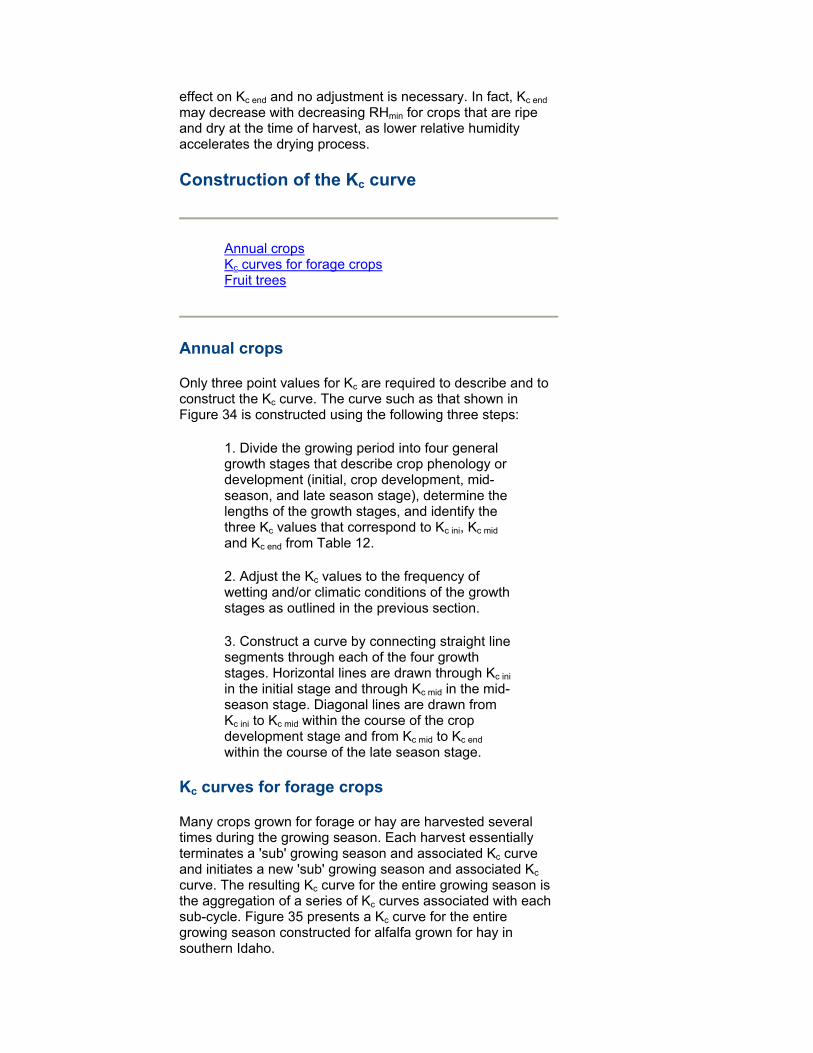
Only three point values for Kc are required to describe and to construct the Kc curve. The curve such as that shown in Figure 34 is constructed using the following three steps:
1. Divide the growing period into four general growth stages that describe crop phenology or development (initial, crop development, mid-season, and late season stage), determine the lengths of the growth stages, and identify the three Kc values that correspond to Kc ini, Kc mid and Kc end from Table 12.
2. Adjust the Kc values to the frequency of wetting and/or climatic conditions of the growth stages as outlined in the previous section.
3. Construct a curve by connecting straight line segments through each of the four growth stages. Horizontal lines are drawn through Kc ini in the initial stage and through Kc mid in the mid-season stage. Diagonal lines are drawn from Kc ini to Kc mid within the course of the crop development stage and from Kc mid to Kc end within the course of the late season stage.
Kc curves for forage crops
Many crops grown for forage or hay are harvested several times during the growing season. Each harvest essentially terminates a 'sub' growing season and associated Kc curve and initiates a new 'sub' growing season and associated Kc curve. The resulting Kc curve for the entire growing season is the aggregation of a series of Kc curves associated with each sub-cycle. Figure 35 presents a Kc curve for the entire growing season constructed for alfalfa grown for hay in southern Idaho.

FIGURE 35. Constructed curve for Kc for alfalfa hay in southern Idaho, the United States using values from
Tables 11 and 12 and adjusted using Equations 62 and 65 (data from Wright, 1990)
In the southern Idaho climate, greenup (leaf initiation) begins in the spring on about day 90 of the year. The crop is usually harvested (cut) for hay three or four times during the growing season. Therefore, Figure 35 shows four Kc sub-cycles or cutting cycles: sub-cycle 1 follows greenup in the spring and the three additional Kc sub-cycles follow cuttings. Cuttings create a ground surface with less than 10% vegetation cover. Cutting cycle 1 is longer in duration than cycles 2, 3 and 4 due to lower air and soil temperatures during this period that reduce crop growth rates. The lengths for cutting cycle 1 were taken from the first entry for alfalfa (" 1st cutting cycle") in Table 11 for Idaho, the United States (10/30/25/10). The lengths for cutting cycles 2, 3 and 4 were taken from the entry for alfalfa in Table 11 for "individual cutting periods" for Idaho, the United States (5/20/10/10). These lengths were based on observations. In the southern Idaho climate, frosts terminate the growing season sometime in the fall, usually around day 280-290 of the year (early to mid-October). The magnitudes of the Kc values during the mid-season periods of each cutting cycle shown in Figure 35 vary from cycle to cycle due to the effects of adjusting the values for Kc
mid and Kc end for each cutting cycle period using Equations 62 and 65. In applying these two adjustment equations, the u2 and RHmin values were averages for the mid-season and late season stages within each cutting cycle. Basal Kcb curves similar to Figure 35 can be constructed for forage or hay crops, following procedures presented in Chapter 7. Kc mid when effects of individual cutting periods are averaged
Under some conditions, the user may wish to average the effects of cuttings for a forage crop over the course of the growing season. When cutting effects are averaged, then only a single value for Kc mid and a only single Kc curve need to be employed for the whole growing season. When this is the case, a "normal" Kc curve is constructed as in Figure 25, where only one midseason period is shown for the forage crop. The Kc mid for this total midseason period must average the effects of occasional cuttings or harvesting. The value that is used for Kc mid is therefore an average of the Kc curve for the time period starting at the first attainment of full cover and ending at the beginning of the final late season period near dormancy or frost. The value used for Kc mid under these averaged conditions may be only about 80% of the Kc value that represents full ground cover. These averaged, full-season Kc mid values are listed in Table 12. For example, for alfalfa hay, the averaged, full-season Kc mid is 1.05, whereas, the Kc
mid for an individual cutting period is 1.20.
Fruit trees
Values for the crop coefficient during the mid-season and end of late season stages are given in Table 12. As mentioned before, the Kc values listed are typical values for standard climatic conditions and need to be adjusted by using Equations 62 and 65 where RHmin or u2 differ. As the mid and late season stages of deciduous trees are quite long, the specific adjustment of Kc to RHmin and u2 should take into account the varying climatic conditions throughout the season. Therefore, several adjustments of Kc are often required if the mid and late seasons cover several climatic seasons, e.g., spring, summer and autumn or wet and dry seasons. The Kc ini and Kc end for evergreen non dormant trees and shrubs are often not different, where climatic conditions do not vary much, as happens in tropical climates. Under these conditions, seasonal adjustments for climate may therefore not be required since variations in ETc depend mostly on variations in ETo.
Calculating ETc
Graphical determination of Kc Numerical determination of Kc
From the crop coefficient curve the Kc value for any period during the growing period can be graphically or numerically determined. Once the Kc values have been derived, the crop evapotranspiration, ETc, can be calculated by multiplying the Kc values by the corresponding ETo values.
Graphical determination of Kc
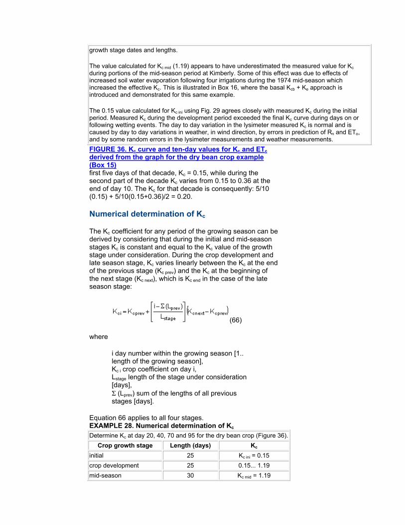
Weekly, ten-day or monthly values for Kc are necessary when ETc calculations are made on weekly, ten-day or monthly time steps. A general procedure is to construct the Kc curve, overlay the curve with the lengths of the weeks, decade or months, and to derive graphically from the curve the Kc value for the period under consideration (Figure 36). Assuming that all decades have a duration of 10 days facilitates the derivation of Kc and introduces little error into the calculation of ETc. The constructed Kc curve in Box 15 was used to construct the curve in Figure 36. This curve has been overlaid with the lengths of the decades. Kc values of 0.15, 1.19 and 0.35 and the actual lengths for growth stages equal to 25, 25, 30 and 20 days were used. The crop was planted at the beginning of the last decade of May and was harvested 100 days later at the end of August. For all decades the Kc values can be derived directly from the curve. The value at the middle of the decade is considered to be the average Kc of that 10 day period. Only the second decade of June, where the Kc value changes abruptly, requires some calculation.
BOX 15. Case study of a dry bean crop at Kimberly, Idaho, the United States (single crop coefficient)
An example application for using the Kc procedure under average soil wetness conditions is presented for a dry bean crop planted on 23 May 1974 at Kimberly, Idaho, the United States (latitude = 42.4°N). The initial, development, mid-season and late season stage lengths are taken from Table 11 for a continental climate as 20, 30, 40 and 20 days (the stage lengths listed for southern Idaho were not used in this example in order to demonstrate the only approximate accuracy of values provided in Table 11 when values for the specific location are not available). Initial values for Kc ini, Kc
mid and Kc end are selected from Table 12 as 0.4, 1.15, and 0.35.
The mean RHmin and u2 during both the mid-season and late season growth stages were 30% and 2.2 m/s. The maximum height suggested in Table 12 for dry beans is 0.4 m. Therefore, Kc mid is adjusted using Eq. 62 as:
As Kc end = 0.35 is less than 0.45, no adjustment is made to Kc end. The value for Kc mid is not significantly different from that in Table 12 as u2 ≈ 2 m/s, RHmin is just 15% lower than the 45% represented in Table 12, and the height of the beans is relatively short. The initial Kc curve for dry beans in Idaho can be drawn, for initial, planning purposes, as shown in the graph (dotted line), where Kc ini, Kc mid and Kc end are 0.4, 1.19 and 0.35 and the four lengths of growth stages are 20, 30, 40 and 20 days. Note that the Kc ini = 0.4 taken from Table 12 serves only as an initial, approximate estimate for Kc ini.
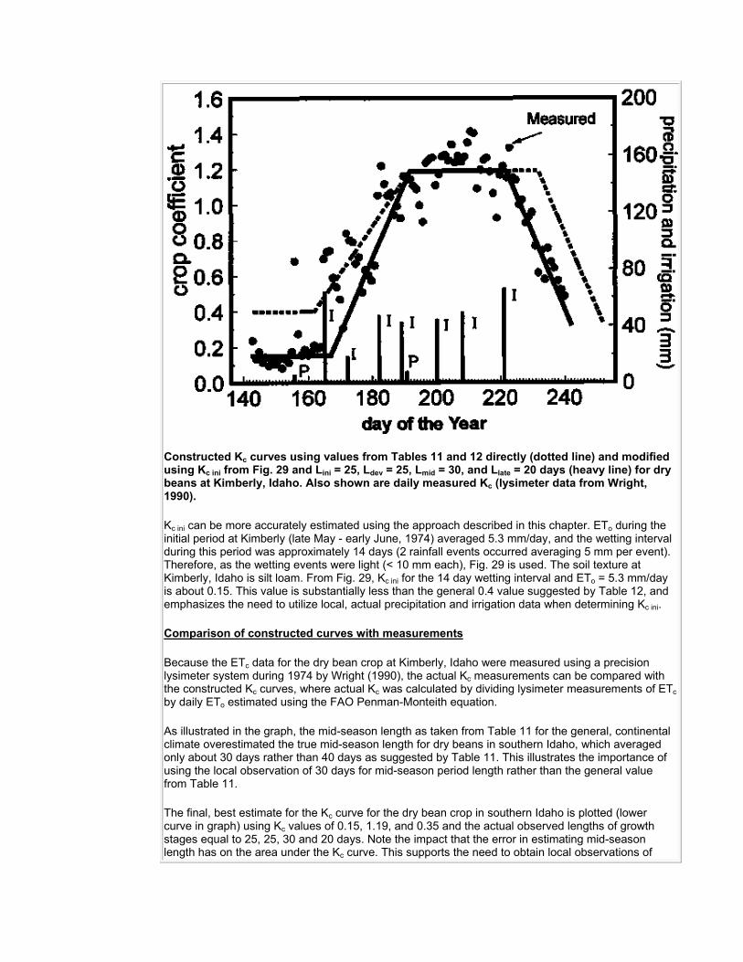
Constructed Kc curves using values from Tables 11 and 12 directly (dotted line) and modified using Kc ini from Fig. 29 and Lini = 25, Ldev = 25, Lmid = 30, and Llate = 20 days (heavy line) for dry beans at Kimberly, Idaho. Also shown are daily measured Kc (lysimeter data from Wright, 1990).
Kc ini can be more accurately estimated using the approach described in this chapter. ETo during the initial period at Kimberly (late May - early June, 1974) averaged 5.3 mm/day, and the wetting interval during this period was approximately 14 days (2 rainfall events occurred averaging 5 mm per event). Therefore, as the wetting events were light (< 10 mm each), Fig. 29 is used. The soil texture at Kimberly, Idaho is silt loam. From Fig. 29, Kc ini for the 14 day wetting interval and ETo = 5.3 mm/day is about 0.15. This value is substantially less than the general 0.4 value suggested by Table 12, and emphasizes the need to utilize local, actual precipitation and irrigation data when determining Kc ini.
Comparison of constructed curves with measurements
Because the ETc data for the dry bean crop at Kimberly, Idaho were measured using a precision lysimeter system during 1974 by Wright (1990), the actual Kc measurements can be compared with the constructed Kc curves, where actual Kc was calculated by dividing lysimeter measurements of ETc
by daily ETo estimated using the FAO Penman-Monteith equation.
As illustrated in the graph, the mid-season length as taken from Table 11 for the general, continental climate overestimated the true mid-season length for dry beans in southern Idaho, which averaged only about 30 days rather than 40 days as suggested by Table 11. This illustrates the importance of using the local observation of 30 days for mid-season period length rather than the general value from Table 11.
The final, best estimate for the Kc curve for the dry bean crop in southern Idaho is plotted (lower curve in graph) using Kc values of 0.15, 1.19, and 0.35 and the actual observed lengths of growth stages equal to 25, 25, 30 and 20 days. Note the impact that the error in estimating mid-season length has on the area under the Kc curve. This supports the need to obtain local observations of
growth stage dates and lengths.
The value calculated for Kc mid (1.19) appears to have underestimated the measured value for Kc during portions of the mid-season period at Kimberly. Some of this effect was due to effects of increased soil water evaporation following four irrigations during the 1974 mid-season which increased the effective Kc. This is illustrated in Box 16, where the basal Kcb + Ke approach is introduced and demonstrated for this same example.
The 0.15 value calculated for Kc ini using Fig. 29 agrees closely with measured Kc during the initial period. Measured Kc during the development period exceeded the final Kc curve during days on or following wetting events. The day to day variation in the lysimeter measured Kc is normal and is caused by day to day variations in weather, in wind direction, by errors in prediction of Rn and ETo, and by some random errors in the lysimeter measurements and weather measurements.
FIGURE 36. Kc curve and ten-day values for Kc and ETc derived from the graph for the dry bean crop example (Box 15) first five days of that decade, Kc = 0.15, while during the second part of the decade Kc varies from 0.15 to 0.36 at the end of day 10. The Kc for that decade is consequently: 5/10 (0.15) + 5/10(0.15+0.36)/2 = 0.20.
Numerical determination of Kc
The Kc coefficient for any period of the growing season can be derived by considering that during the initial and mid-season stages Kc is constant and equal to the Kc value of the growth stage under consideration. During the crop development and late season stage, Kc varies linearly between the Kc at the end of the previous stage (Kc prev) and the Kc at the beginning of the next stage (Kc next), which is Kc end in the case of the late season stage:
(66)
where
i day number within the growing season [1.. length of the growing season], Kc i crop coefficient on day i, Lstage length of the stage under consideration [days], Σ (Lprev) sum of the lengths of all previous stages [days].
Equation 66 applies to all four stages. EXAMPLE 28. Numerical determination of Kc
Determine Kc at day 20, 40, 70 and 95 for the dry bean crop (Figure 36).
Crop growth stage Length (days) Kc
initial 25 Kc ini = 0.15
crop development 25 0.15... 1.19
mid-season 30 Kc mid = 1.19
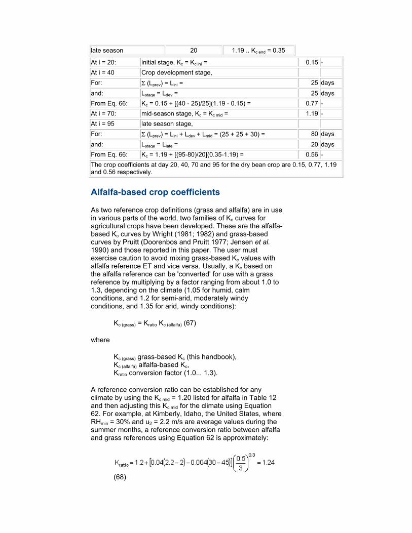
late season 20 1.19 .. Kc end = 0.35
At i = 20: initial stage, Kc = Kc ini = 0.15 -
At i = 40 Crop development stage,
For: Σ (Lprev) = Lini = 25 days
and: Lstage = Ldev = 25 days
From Eq. 66: Kc = 0.15 + [(40 - 25)/25](1.19 - 0.15) = 0.77 -
At i = 70: mid-season stage, Kc = Kc mid = 1.19 -
At i = 95 late season stage,
For: Σ (Lprev) = Lini + Ldev + Lmid = (25 + 25 + 30) = 80 days
and: Lstage = Llate = 20 days
From Eq. 66: Kc = 1.19 + [(95-80)/20](0.35-1.19) = 0.56 -
The crop coefficients at day 20, 40, 70 and 95 for the dry bean crop are 0.15, 0.77, 1.19 and 0.56 respectively.
Alfalfa-based crop coefficients
As two reference crop definitions (grass and alfalfa) are in use in various parts of the world, two families of Kc curves for agricultural crops have been developed. These are the alfalfa-based Kc curves by Wright (1981; 1982) and grass-based curves by Pruitt (Doorenbos and Pruitt 1977; Jensen et al. 1990) and those reported in this paper. The user must exercise caution to avoid mixing grass-based Kc values with alfalfa reference ET and vice versa. Usually, a Kc based on the alfalfa reference can be 'converted' for use with a grass reference by multiplying by a factor ranging from about 1.0 to 1.3, depending on the climate (1.05 for humid, calm conditions, and 1.2 for semi-arid, moderately windy conditions, and 1.35 for arid, windy conditions):
Kc (grass) = Kratio Kc (alfalfa) (67)
where
Kc (grass) grass-based Kc (this handbook), Kc (alfalfa) alfalfa-based Kc, Kratio conversion factor (1.0... 1.3).
A reference conversion ratio can be established for any climate by using the Kc mid = 1.20 listed for alfalfa in Table 12 and then adjusting this Kc mid for the climate using Equation 62. For example, at Kimberly, Idaho, the United States, where RHmin = 30% and u2 = 2.2 m/s are average values during the summer months, a reference conversion ratio between alfalfa and grass references using Equation 62 is approximately:
(68)
where
h = 0.5 m is the standard height for the alfalfa reference.
Transferability of previous Kc values
The values for Kc mid and Kc end listed in Table 12 are for a large part based on the original values presented in FAO Irrigation and Drainage Papers No. 24 and 33 (FAO-24 and FAO-33), with some adjustment and revisions to reflect recent findings. Similarly adjustments in Kc mid to compensate for differences in aerodynamic roughness and leaf area, as introduced in Equation 62 are derived from the Kc values given for different wind and RHmin conditions in the concerned Kc table in FAO-24, with some upward adjustment to better reflect increased ETcrop values under high wind and low RHmin when applied with the FAO Penman-Monteith equation. The Kc's from FAO-24 were based primarily on a living grass reference crop. The FAO Penman-Monteith equation presented in this publication similarly represents the same standardized grass reference. For that reason Kc values are in general not very different between these publications except under high wind and low RHmin. The No. 24 modified Penman was found frequently to overestimate ETo even up to 25 % under high wind and low evaporative conditions and required often substantial local calibration (see chapter 2). Kc values derived from crop water use studies which used the FAO-24 Penman equation to compute grass reference crop evapotranspiration, can therefore not be used and need to be adjusted using ETo values estimated from the FAO Penman-Monteith equation. Similarly crop water requirement estimates based on the FAO-24 Modified Penman equation will need to be reassessed in view of the found differences between the FAO-24 Penman and the FAO Penman-Monteith reference equations.