458

Interlude(Optimization and other Numerical Methods)

Fish 458, Lecture 8

458

Numerical Methods Most fisheries assessment problems are

mathematically too complicated to apply analytical methods. We often have to resort to numerical methods. The two most frequent questions requiring numerical solutions are:

Find the values for a set of parameters so that they satisfy a set of (non-linear) equations.

Find the values for a set of parameters to minimize some function.

Note: Numerical methods can (and do) fail – you need to know enough about them to be able to check for failure.

458

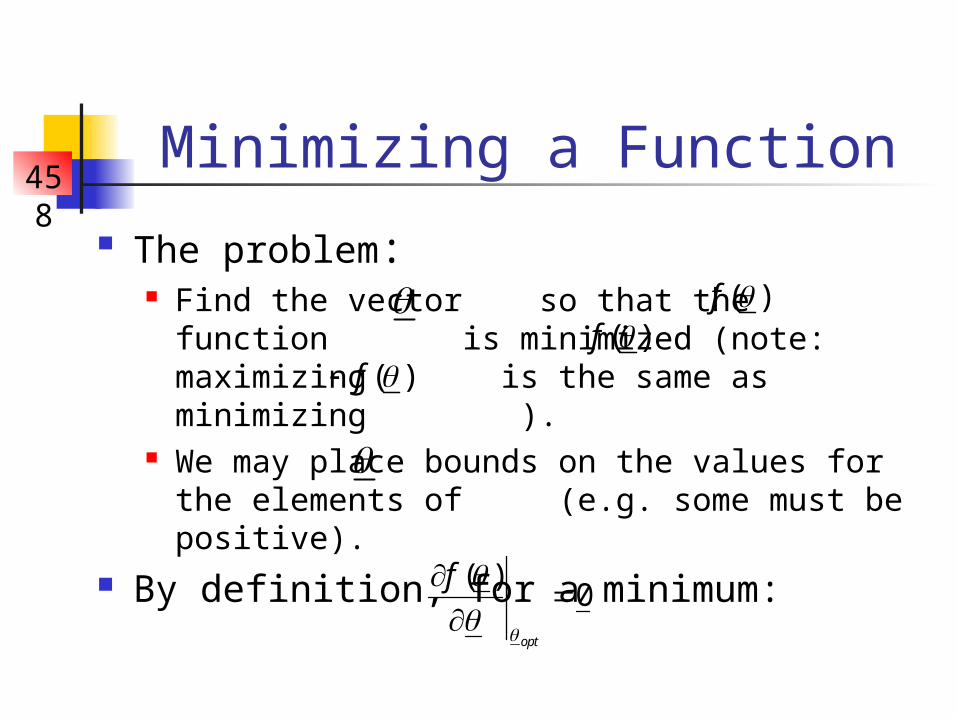
Minimizing a Function The problem:

Find the vector so that the function is minimized (note: maximizing is the same as minimizing ).

We may place bounds on the values for the elements of (e.g. some must be positive).

By definition, for a minimum:

( )f ( )f

( )f

( )0

opt

f

458

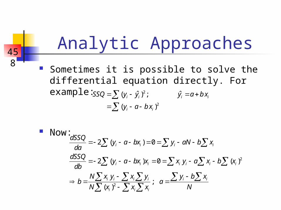
Analytic Approaches Sometimes it is possible to solve the

differential equation directly. For example:

Now:

2

2

ˆ ˆ( ) ;

( )

i i i i

i i

SSQ y y y a b x

y a b x

2

2

2 ( ) 0

2 ( ) 0 ( )

;( )

i i i i

i i i i i i i

i i i i i i

i i i

dSSQy a bx y aN b x

dadSSQ

y a bx x x y a x b xdb

N x y x y y b xb a

N x x x N

458

Linear Models – The General Case

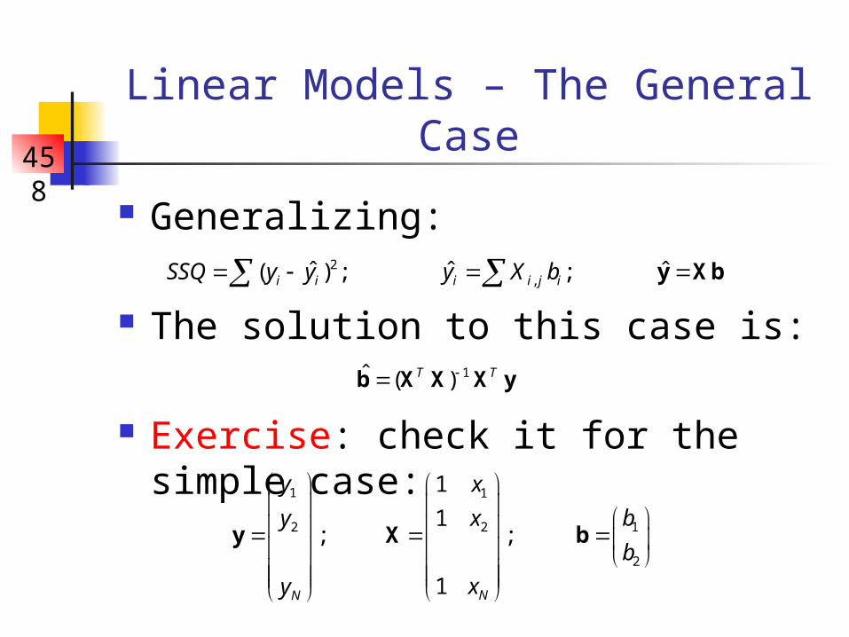
Generalizing:

The solution to this case is:

Exercise: check it for the simple case:

2,ˆ ˆ ˆ( ) ; ;i i i i j iSSQ y y y X b y Xb

1ˆ ( )T Tb X X X y

1 1

12 2

2

1

1; ;

1 NN

y x

by x

b

xy

y X b

458

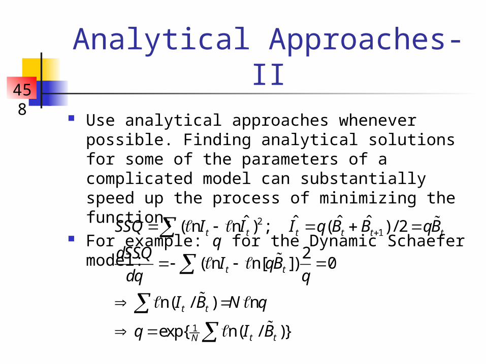
Analytical Approaches-II Use analytical approaches whenever possible.

Finding analytical solutions for some of the parameters of a complicated model can substantially speed up the process of minimizing the function.

For example: q for the Dynamic Schaefer model:

21

1

ˆ ˆ ˆ ˆ( n n ) ; ( ) / 2

2( n n[ ]) 0

n( / ) n

exp{ n( / )}

t t t t t t

t t

t t

t tN

SSQ I I I q B B qB

dSSQI qB

dq q

I B N q

q I B

458

Numerical Methods (Newton’s Method)

Single variable version-I

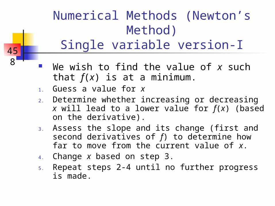
We wish to find the value of x such that f(x) is at a minimum.

1. Guess a value for x2. Determine whether increasing or decreasing x

will lead to a lower value for f(x) (based on the derivative).

3. Assess the slope and its change (first and second derivatives of f) to determine how far to move from the current value of x.

4. Change x based on step 3.5. Repeat steps 2-4 until no further progress is

made.

458

Numerical Methods (Newton’s Method)

Single variable version-II

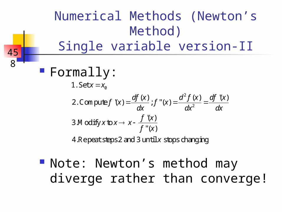
Formally:

Note: Newton’s method may diverge rather than converge!

0

2

2

1. Set

( ) ( ) '( )2. Compute '( ) ; "( )

'( )3.Modify to

"( )

4.Re peat steps 2 and 3 until stops changing

x x

df x d f x df xf x f x

dx dx dxf x

x x xf x

x

458

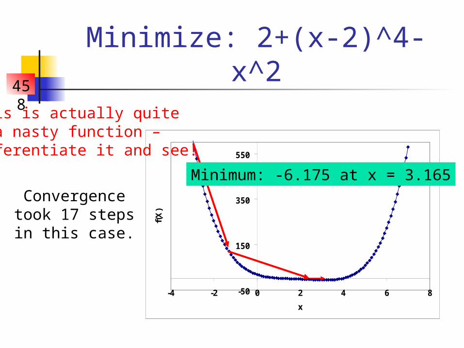
Minimize: 2+(x-2)^4-x^2

-50

150

350

550

-4 -2 0 2 4 6 8

x

f(X

)

This is actually quite a nasty function –

differentiate it and see!

Convergence took 17 steps in this case.

Minimum: -6.175 at x = 3.165

458

Numerical Methods (Newton’s Method)

If the function is quadratic (i.e. the third derivative is zero), Newton’s method will get to the solution in one step (but then you could solve the equation by hand!)

If the function is non-quadratic, iteration will occur.

Multi-parameter extensions to Newton’s method exist but most people prefer gradient free methods (e.g. SIMPLEX) to deal with problems like this.

458

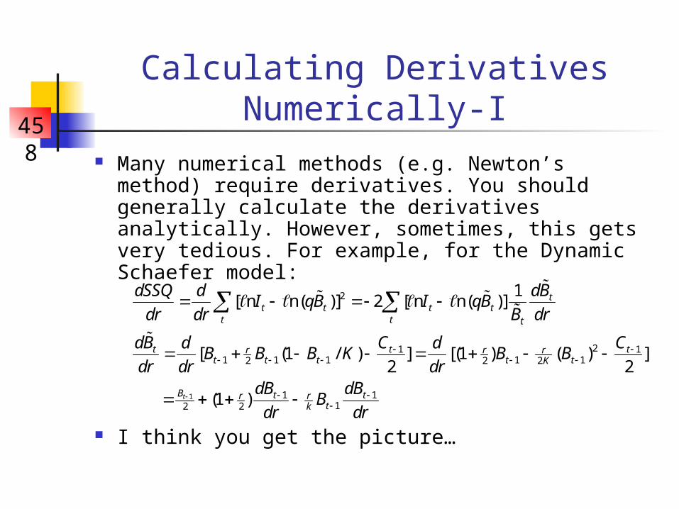
Calculating Derivatives Numerically-I

Many numerical methods (e.g. Newton’s method) require derivatives. You should generally calculate the derivatives analytically. However, sometimes, this gets very tedious. For example, for the Dynamic Schaefer model:

I think you get the picture…

1

2

21 11 1 1 1 12 2 2

1 112 2

1[ n n( )] 2 [ n n( )]

[ (1 / ) ] [(1 ) ( ) ]2 2

(1 )t

tt t t t

t t t

t t tr r rt t t t tK

B t tr rtk

dBdSSQ dI qB I qB

dr dr B dr

dB C Cd dB B B K B B

dr dr drdB dB

Bdr dr

458

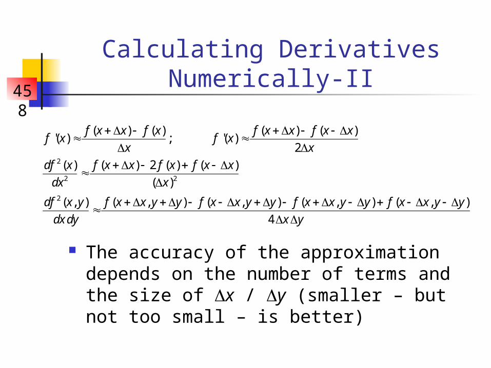
Calculating Derivatives Numerically-II

The accuracy of the approximation depends on the number of terms and the size of x / y (smaller – but not too small – is better)

2

2 2

2

( ) ( ) ( ) ( )'( ) ; '( )

2

( ) ( ) 2 ( ) ( )

( )

( , ) ( , ) ( , ) ( , ) ( , )

4

f x x f x f x x f x xf x f x

x x

df x f x x f x f x x

dx x

df x y f x x y y f x x y y f x x y y f x x y y

dx dy x y

458

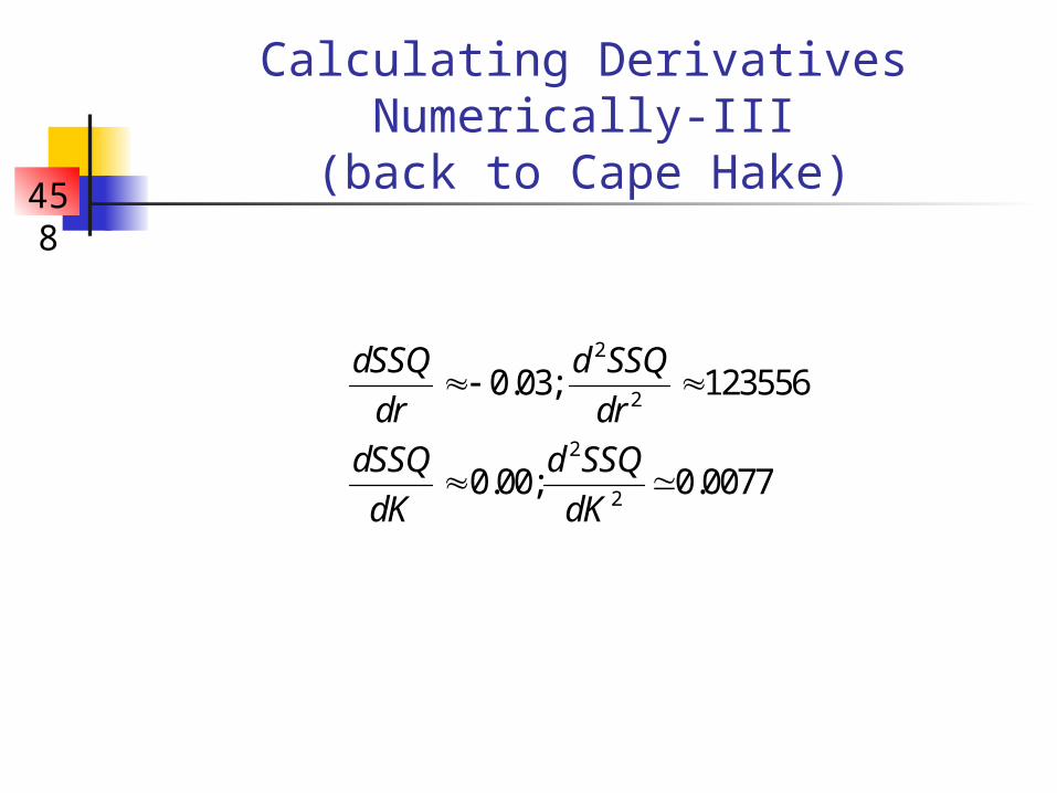
Calculating Derivatives Numerically-III

(back to Cape Hake)

2

2

2

2

0.03; 123556

0.00; 0.0077

dSSQ d SSQ

dr dr

dSSQ d SSQ

dK dK

458

Optimization – some problems-I

Local minima

-3000

-2000

-1000

0

1000

2000

-6 -4 -2 0 2 4 6

X

f(X

)

Global minimum

Local minimum

458

Optimization – some problems-II

Problems calculating numerical derivatives.

Integer parameters. Bounds [either on the function

itself (extinction of Cape Hake hasn’t happened - yet) or on the values for the parameters].

458

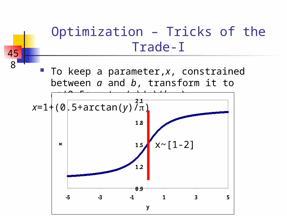
Optimization – Tricks of the Trade-I

To keep a parameter,x, constrained between a and b, transform it to a+(0.5+arctan(y)/)(b-a).

0.9

1.2

1.5

1.8

2.1

-5 -3 -1 1 3 5

y

x

x=1+(0.5+arctan(y)/)

x~[1-2]

458

Optimization – Tricks of the Trade-II

Test the code for the model by fitting to data where the answer is known!

Look at the fit graphically (have you maximized rather than minimizing the function)?

Minimize the function manually; restart the optimization algorithm from the final value; restart the optimization algorithm from different values.

When fitting n parameters that must add to 1, fit n-1 parameters and set the last to 1-sum(1:n-1).

In SOLVER, use automatic scaling and set the convergence criterion smaller.

458

Solving an Equation(the Bisection Method)

Often we have to solve the equation f(x)=0 (e.g. the Lokta equation). This can be treated as an optimization problem (i.e. minimize f(x)2).

However, it is usually more efficient to use a numerical method specifically developed for this purpose.

We illustrate the Bisection Method here but there are many others.

458

Solving an Equation(the Bisection Method)

1 2 1 2

1 2

1

2

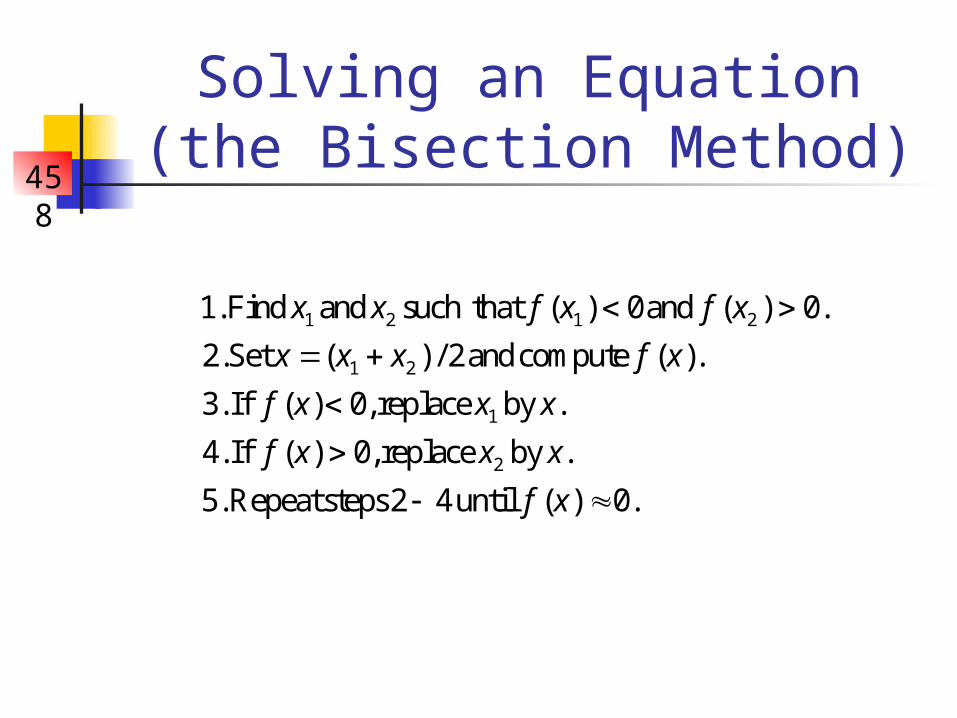
1.Find and such that ( ) 0and ( ) 0.

2.Set ( ) / 2and compute ( ).

3. If ( ) 0, replace by .

4. If ( ) 0, replace by .

5.Repeat steps2 4 until ( ) 0.

x x f x f x

x x x f x

f x x x

f x x x

f x

458

Solving an Equation(the Bisection Method)

-100

0

100

200

300

400

500

4 9 14 19

Step Number

F(x

)

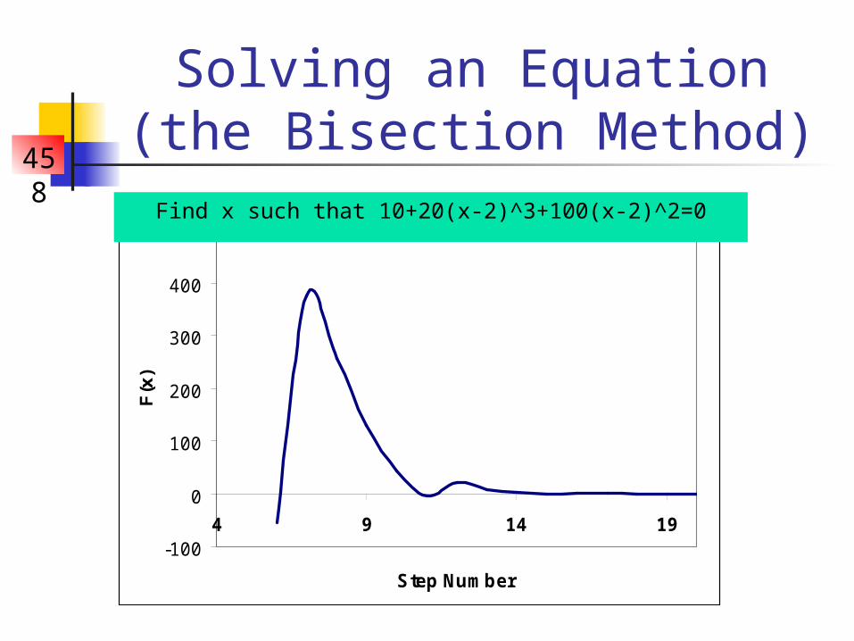
Find x such that 10+20(x-2)^3+100(x-2)^2=0

458

Note Use of Numerical Methods

(particularly optimization) is an art. The only way to get it right is to practice (probably more than anything else in this course).

458

Readings Hilborn and Mangel (1997);

Chapter 11 Press et al. (1988), Chapter 10