1

Modules 4, 5, 6 / Topic 4

EARTH PRESSURES

4.1 Introduction

A retaining structure, such s a retaining wall, retains (holds in place) soil on one side

(Fig. 4.1). The lateral pressure exerted by the retained soil on the wall is called earth

pressure. It is necessary for us to quantitatively determine these pressures as they

constitute the loading on the wall for which it must be designed both geotechnically and

structurally, the former ensuring the various aspects of stability of the wall (stability

analysis) and the latter, catering to the structural action induced in the wall by the forces

(Kurian, 2005: Sec.1.1.2). Since we deal with the limiting values of these pressures, earth

pressures are ultimate problems in Soil Mechanics. This means, at this stage the soil is

no longer in a state of elastic equilibrium, but has reached the stage of plastic equilibrium.

In situations such as the one shown in Fig. 4.2, which involves grading (removal) and

filling, the in-situ soil itself may be used as the fill. The soil which thus stays in contact

with the wall is called backfill in the sense of being the fill at the back of the wall or a fill

which is put back. However, where we have the choice for a fresh backfill material, we

would go in for cohesionless soils of high internal friction (ϕ), and permeability (k) to aid

fast drainage (Kurian, 2005: Sec.6.1).

A retaining wall permits a backfill with a vertical face. The alternative to a retaining wall

to secure the sides is to provide a wide slope (Fig. 4.3) as, for example, in road

embankments, but this needs the availability of adequate land to ensure the desired level

of stability of slopes, which may not be available in all instances. It may be noted in this

connection that sometimes backfills may themselves be laid in slopes to reduce the

heights of the wall (Fig. 4.4).

It is ideal that the water table (free water level in soil) stays below the base of the wall

without allowing it to rise into the backfill, adding to the load on the wall – with water

pressure adding to the earth pressure from the submerged soil below the water table –

for which it may not have been designed, rendering the design inadequate in such

eventualities. However, in situations such as water-front structures (Fig. 4.5), we have to

reckon with water, since water table will eventually rise in the backfill and attain the same

level as the free water in the front.

We shall first consider earth pressure due to dry backfills.

4.2 The limiting values of earth pressures

2

Earth pressures attain their ultimate or ‘limiting’ values depending on the relative

movement of the wall with respect to the backfill.

Thus from a stationary position, if the wall starts moving away from the soil, the

pressure exerted by the soil on the wall starts decreasing until a stage is reached when

the pressure reaches its lowest value (Fig.4.6). This means that there will be no further

reduction in the pressure, if the wall moves further away from the soil. This limiting

pressure is called active earth pressure.

On the other hand, if the wall is made to move towards the soil, i.e. the wall pushes

the soil, the pressure exerted by the soil on the wall starts increasing until a stage is

reached when the pressure attains its maximum value (Fig.4.6) and as before, there will

be no further increase in the pressure if the wall moves further towards the soil. This

limiting pressure is called the passive earth pressure. In the initial at-rest state, the soil

is in a state of elastic equilibrium. From this state it reaches the states of plastic

equilibrium at the limiting active and passive states. The initial value of the earth pressure

may be called neutral earth pressure or earth pressure at-rest.

Fig. 4.7 shows quantitatively typical at-rest, active and passive earth pressure

distributions on the retaining wall. While the active pressure is about 2/3 of the at-rest

value, the passive pressure is nearly 6 times the at-rest value, or 9 times the active value

in a cohesionless soil with ϕ = 300. Further, in a similar manner, the passive state is

mobilised at a much higher value of wall movement than the active state. Quantitatively,

the lateral wall movements are typically 0.25 % and 3.5 % of the wall height for the active

and passive pressure conditions to get fully mobilised, respectively (Venkatramaiah,

2006: Sec. 13.3).

A word of explanation is due with regard to the names active and passive. In the active

case, soil is the actuating element the movement of which leading to the active condition.

In the passive case, the actuating element is the wall leading the soil to a passive state

of resistance against the approaching wall (Venkatramaiah, 2006: Sec. 13.3).

4.3 Determination of earth pressures by earth pressure theories

Earth pressures are determined by earth pressure theories. The two basic theories

available for this purpose are the Rankine’s theory and the Coulomb’s theory. Of the two,

the Coulomb’s theory is the older one; we shall, however, take up the Rankine’s theory

first because of its theoretical form.

However, before setting out on the above theories of limiting earth pressures, it is

necessary for us to look at earth pressure at-rest which should be treated as a starting

case. The soil being in elastic equilibrium at this stage, we should be able to proceed

with it based on theory of elasticity considerations.

3

4.4 Earth pressure at rest

Fig. 4.8 shows an element of soil at a depth z in a semi-infinite soil mass. (Semi-

infinite means the mass extends in the +x, -x, +y, -y directions, but only in the +z

(downward) directions, all to infinity. If it extends equally also in the –z direction (upwards)

it would have made a fully infinite space.) The vertical and horizontal stresses in the

element are shown. The element can deform (undergo strain) in the vertical direction

only since the soil extends to infinity in the horizontal directions. Let the modulus of

elasticity and Poisson’s ratio of the soil be 𝛦𝑠 and μ respectively. Setting the lateral strain,

obtained from theory of elasticity to 0,

𝜖ℎ = 𝜎𝑣

𝐸𝑠 - μ (

𝜎𝑣

𝐸𝑠 +

𝜎ℎ

𝐸𝑠 ) = 0 (4.1)

Multiplying by 𝛦𝑠

𝜎ℎ - μ (𝜎𝑣 + 𝜎ℎ) = 0

𝜎ℎ(1- μ) = μ𝜎𝑣

𝜎ℎ

𝜎𝑣 =

𝜇

1− 𝜇 (4.2)

Referring to Fig 4.8

𝜎𝑣 = 𝛾. 𝑧

Therefore 𝜎ℎ = ( 𝜇

1− 𝜇 ) 𝛾. 𝑧

If ( 𝜇

1− 𝜇 ) is denoted as 𝐾0 and named coefficient of earth pressure at-rest, we can

set

𝜎ℎ = 𝐾0 𝛾. 𝑧 (4.3)

𝐾0 being a constant, it is noted that 𝜎ℎ also increases linearly with depth as 𝜎𝑣 itself,

starting with 0 at the surface (z = 0)

If we now revert to Topic 1, it is seen that the 𝐾0- μ relationship is of the same form as

the e-n relationship. Hence 𝐾0 will plot against 𝜇 as in Fig. 1.3.

4

We note that 𝐾0 = 0 when μ = 0, a condition giving rise to 0 horizontal pressure.

Further setting 𝐾0 = 1,

𝜇

1−𝜇= 1

μ = 1-μ

2μ = 1

μ = 1

2

At this value of μ, 𝜎ℎ = 𝜎𝑣 = 𝛾. 𝑧

or in other words, 𝜎ℎ and 𝜎𝑣 will plot identically with depth. When μ varies from 0 to 0.5,

𝜎ℎ will vary as increasing fractions of 𝜎𝑣, as can be noted from Fig. 4.9.

Because of the difficulty in determining μ of a soil reliably, various empirical formulae

have been suggested among which the one attributed to Jaky (1944) is an early favourite.

It states: 𝐾0 = 1 − 𝑠𝑖𝑛𝜙 (4.4)

Fig 4.10 plots 𝐾0 against 𝜙. It bears comparison with Fig. 16 (Kurian, 2005: Sec. 6.4.1)

for which it is plotted till 𝜙 = 900. It is noted from Figs. 4.9 and 4.10 that 𝐾0 increases with

μ, but decreases with 𝜙. At 𝜙 = 0, applying to water, 𝐾0 = 1, following which 𝜎𝑣 = 𝜎ℎ.

On the other hand, at 𝜙= 900, applying to rock, 𝐾0 = 𝜎ℎ = 0

4.5 Rankine’s theory for active and passive earth pressures (1857)

Before we take up Rankine’s theory of earth pressure, we shall try to establish

analytically the relationship between 𝜎1 𝑎𝑛𝑑 𝜎3, the principal stresses, based on the

Mohr-Coulomb failure theory (Fig.4.11).

In the figure,

CA = CD = 𝜎1−𝜎3

2

OC = OA+AC = 𝜎3 +𝜎1

2−

𝜎3

2=

𝜎3+𝜎1

2

EO = c cot ϕ

CD = EC sin ϕ

5

i.e., 𝜎1−𝜎3

2= (

𝜎1+𝜎3

2+ 𝑐 𝑐𝑜𝑡 𝜙) 𝑠𝑖𝑛 𝜙

Multiplying by 2

𝜎1−𝜎3 = (𝜎1 + 𝜎3 + 2𝑐 𝑐𝑜𝑡 𝜙) 𝑠𝑖𝑛 𝜙

= (𝜎1 𝑠𝑖𝑛 𝜙 + 𝜎3 𝑠𝑖𝑛 𝜙 + 2𝑐 𝑐𝑜𝑠 𝜙

𝜎1(1 − 𝑠𝑖𝑛 𝜙) = 𝜎3(1 + 𝑠𝑖𝑛 𝜙) + 2𝑐 𝑐𝑜𝑠 𝜙

𝜎1 = 𝜎3 (1+𝑠𝑖𝑛 𝜙

1−𝑠𝑖𝑛 𝜙) + 2𝑐

𝑐𝑜𝑠 𝜙

1−𝑠𝑖𝑛 𝜙

Similarly, 𝜎3 = 𝜎1 (1−𝑠𝑖𝑛 𝜙

1+𝑠𝑖𝑛 𝜙) − 2𝑐

𝑐𝑜𝑠 𝜙

1+𝑠𝑖𝑛 𝜙

Trignometrically 1−𝑠𝑖𝑛 𝜙

1+𝑠𝑖𝑛 𝜙= 𝑡𝑎𝑛2(45 −

𝜙

2 )

1+𝑠𝑖𝑛 𝜙

1−𝑠𝑖𝑛 𝜙= 𝑡𝑎𝑛2(45 +

𝜙

2 )

𝑐𝑜𝑠 𝜙

1+𝑠𝑖𝑛 𝜙= 𝑡𝑎𝑛 (45 +

𝜙

2)

𝑐𝑜𝑠 𝜙

1−𝑠𝑖𝑛 𝜙= 𝑡𝑎𝑛 (45 +

𝜙

2)

Hence we can state

𝜎3 = 𝜎1𝑡𝑎𝑛2 (45 −𝜙

2) − 2𝑐 𝑡𝑎𝑛 (45 −

𝜙

2) (4.5)

𝜎1 = 𝜎3𝑡𝑎𝑛2 (45 +𝜙

2) + 2𝑐 𝑡𝑎𝑛 (45 +

𝜙

2) (4.6)

Referring to Fig. 4.11, one may look upon the c-ϕ case as the ϕ -case with the origin

shifting from E to O.

4.5.1 Rankine’s expressions for active and passive earth pressures

In Fig. 4.12 let OA represent the vertical (principal) stress. Mohr’s circles I and II are

drawn on either side of A without gap. In case I the soil is laterally relieved leading to

reduction in 𝜎ℎ − reaching 𝜎𝑎 − the limiting active value at failure. In case II the soil is

pushed into itself and 𝜎ℎ reaches the limiting passive value of 𝜎𝑝 at failure.

6

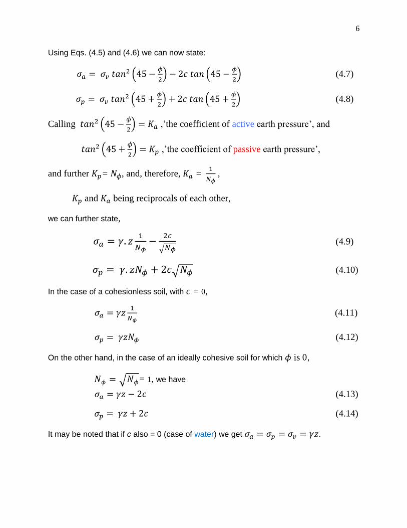
Using Eqs. (4.5) and (4.6) we can now state:

𝜎𝑎 = 𝜎𝑣 𝑡𝑎𝑛2 (45 −𝜙

2) − 2𝑐 𝑡𝑎𝑛 (45 −

𝜙

2) (4.7)

𝜎𝑝 = 𝜎𝑣 𝑡𝑎𝑛2 (45 +𝜙

2) + 2𝑐 𝑡𝑎𝑛 (45 +

𝜙

2) (4.8)

Calling 𝑡𝑎𝑛2 (45 −𝜙

2) = 𝐾𝑎 ,’the coefficient of active earth pressure’, and

𝑡𝑎𝑛2 (45 +𝜙

2) = 𝐾𝑝 ,’the coefficient of passive earth pressure’,

and further 𝐾𝑝= 𝑁𝜙, and, therefore, 𝐾𝑎 = 1

𝑁𝜙 ,

𝐾𝑝 and 𝐾𝑎 being reciprocals of each other,

we can further state,

𝜎𝑎 = 𝛾. 𝑧1

𝑁𝜙−

2𝑐

√𝑁𝜙 (4.9)

𝜎𝑝 = 𝛾. 𝑧𝑁𝜙 + 2𝑐√𝑁𝜙 (4.10)

In the case of a cohesionless soil, with c = 0,

𝜎𝑎 = 𝛾𝑧1

𝑁𝜙 (4.11)

𝜎𝑝 = 𝛾𝑧𝑁𝜙 (4.12)

On the other hand, in the case of an ideally cohesive soil for which 𝜙 is 0,

𝑁𝜙 = √𝑁𝜙= 1, we have

𝜎𝑎 = 𝛾𝑧 − 2𝑐 (4.13)

𝜎𝑝 = 𝛾𝑧 + 2𝑐 (4.14)

It may be noted that if c also = 0 (case of water) we get 𝜎𝑎 = 𝜎𝑝 = 𝜎𝑣 = 𝛾𝑧.

7

Note further that, since the plane of failure is inclined at 𝛼 = (45 +𝜙

2), it follows

that 𝐾𝑝 = 𝑡𝑎𝑛2𝛼, 𝐾𝛼 = 1

𝑡𝑎𝑛2𝛼

The above results pertaining to 𝜙 and c-soils can be directly obtained from the respective

Mohr’s circles as shown in Figs. 4.13 and 4.14.

4.5.2 Failure planes

The failure plane in the active state is inclined at 𝛼 = (45 +𝜙

2) to the horizontal. If the

full Mohr’s circle is drawn, the potential failure planes are as shown in Fig. 4.15

(Venkatramaiah, 2006: Sec.13.6.1). In the passive case, like in the active case, the failure

plane should be reckoned from the point 𝜎𝑝. It can be identified that the failure planes at

passive failure are inclined at (45 −𝜙

2) to the horizontal. (The arcs of the Mohr’s circles

subtending these angles are highlighted in Fig. 4.12.) The picture is the same for 𝜙-soil.

In the case of the c-soil, these planes are inclined at 450 to the horizontal.

4.5.3 Variation of active and passive earth pressure coefficients

It follows from the Rankine’s theory that the higher the 𝜙, the higher the shear strength,

the lesser the active pressure and the higher the passive pressure.

It is interesting to note that the Rankine’s theory for earth pressure developed for soil

can be extended to water (ϕ = 0) on the one hand and rock ( ϕ =900), on the other.

When ϕ = 0, 𝐾𝑎 = 𝐾𝑝 = 𝐾𝑜 = 1

Therefore, 𝑝𝑎 = 𝑝𝑝 = 𝑝0 = 𝑝ℎ = 𝑝𝑣 = 𝛾𝑤ℎ

This is the hydrostatic pressure condition, applying to water.

If ϕ increases, 𝐾𝑎 decreases and 𝐾𝑝 increases. The latter increases much faster than the

former decreases, until we reach ϕ = 900 at which 𝐾𝑎= 0 and 𝐾𝑝 = ∞. As a result, 𝑝𝑣 =

𝛾ℎ, 𝑝𝑎= 0 and 𝑝𝑝 = ∞.The variations of 𝐾𝑎 and 𝐾𝑝, and also their square roots, with 𝜙 are

shown in Fig. 4.16.

4.5.4 Plots of 𝑝𝑎 and 𝑝𝑝

c-ϕ case

8

Since c and ϕ are constants, the first part of 𝑝𝑎 and 𝑝𝑝 , as per Eqs. (4.9) and (4.10)

plot linearly like 𝑝𝑣, but the second parts are constants. Fig 4.17 shows the sum of these

effects. (Note that when two plots are to be added they should be drawn on opposite

sides, whereas if one is to be subtracted from the other they should be drawn on the same

side.)

It is observed from Eqs. (4.9) and (4.10) that 𝑝𝑎 is decreased and 𝑝𝑝 is increased on

account of the contribution of c. As a result of the subtraction, Fig 4.16a shows a tensile

zone to a depth z which can be determined by setting,

𝛾𝑧

𝑁𝜙=

2𝑐

√𝑁𝜙

. Therefore 𝑧 =2𝑐

𝛾√𝑁𝜙 (4.15)

Since soil cannot exist in a state of tension, it is likely that it breaks contact with the

support over this depth (Kurian, 2005: Sec. 8.8).

c-case

Fig. 4.18 shows the active and passive pressure variations in the c-case.

To obtain the depth z at which the net pressure is 0,

Setting 𝛾z = 2c, from which z = 2𝑐

𝛾

4.5.5 Effect of surcharge on the backfill

There are instances such as in port and harbour structures where the backfill is

subjected to heavy surcharges such as due to supporting roads, railway tracks and heavy

stationary equipments. Like any other vertical load such as the self weight of the backfill,

these surcharges add to the lateral pressure on the wall the effect of which must be taken

into account in its design.

In order to consider the influence of the surcharge, its effect is reduced to an equivalent

downward pressure, q per unit area, Fig. 4.19.

The lateral active pressure due to surcharge is q𝐾𝑎 which is uniform with depth, q and

𝐾𝑎 being constants. To this will be added the active earth pressure as shown in the figure.

The same figure can be obtained by converting the surcharge pressure q as an

equivalent additional height (h’) of the backfill which is obtained by setting

γ h’ = q, from which h’ = ( 𝑞

𝛾 ) (4.16)

9

The pressure diagram on the wall alone for the full height of the backfill including the

additional height is the same as the earlier pressure diagram as shown in the figure.

4.5.6 Earth pressure due to layered backfills

Rankine’s theory can easily accommodate layered backfills, if the layers concerned

are horizontal.

Let us consider the example shown in Fig. 4.20.

𝑝𝑎 𝑎𝑡 B̅ = 𝛾1 ℎ11

𝑁𝜙1

(4.17)

𝑝𝑎 at B+

= 𝛾1 ℎ11

𝑁𝜙2

−2𝑐

√𝑁𝜙2

(4.18)

𝑝𝑎 at C = (𝛾1ℎ1 + 𝛾2ℎ2)1

𝑁𝜙2

− 2𝑐

√𝑁𝜙2

(4.19)

The above means that there is an immediate transition at B thanks to the difference in the

shear strength parameters of layers I and II. As a result it is seen that 𝑝𝑎 at 𝐵+ undergoes

a sudden decrease thanks to the presence of c, 𝜙 being the same in the present case.

Theoretically speaking, 𝑝𝑎 at B̅ applies to a point in layer I lying infinitesimally above

point B, whereas 𝑝𝑎 at point B+

applies to a point in layer II lying infinitesimally below point

B. If one asks what is its value exactly at point B, the theoretical answer is, it is not the

average of 𝑝𝑎 𝑎𝑡 B̅ and 𝑝𝑎 at 𝐵+

, but, simply, it is not defined at B.

4.5.7 Earth pressure due to submerged backfills

If the backfill is submerged fully or partially, i.e. to full height or partial height, there is

a continuous body of water running through the pore space in the soil below the water

table. The water over this height will exert full hydrostatic pressure on the wall. To this

will be added the pressure due to submerged soil over this depth and the dry soil above

(Fig. 4.21).

While submergence causes a reduction in the unit weight of the soil, the shear strength

parameters c and 𝜙 remain unchanged.

Submerged unit weight (Kurian, 2005: Sec.2.7.1)

The submerged weight of a continuous (i.e. non-porous) body is its weight in air

subtracted by the weight of water displaced by the body. In other words,

10

submerged weight of an object = weight in air of the object - weight of a body of water

having the same volume as the object.

That is to say, ws = w – v.𝛾𝜔 (4.20)

Unit weight is the weight per unit volume. In submerged unit weight 𝛾sub of the soil we

are concerned with is the weight of the solid particles in the soil in a unit volume which

are in a state of submergence.

Fig. 4.22 represents a unit volume in which

𝛾sub = weight of solids – weight of an equal volume of water.

In order to simplify calculation, we add to both the parts on the R.H.S. a constant which

is the water to fill the pore space. The constant being the same, the result is, we have

saturated unit weight as the first term and unit weight of water as the second term on the

R.H.S. The final result is the familiar result,

𝛾𝑠𝑢𝑏 = 𝛾𝑠𝑎𝑡- 𝛾𝑤. (4.21)

Interestingly enough, this follows Eq.(4.20) with 𝛾𝑠𝑎𝑡 in place of w, as it should,

representing the whole body.

4.5.8 Combined pressures (Kurian, 2005: Sec.6.4.2)

What follows is an important matter which every student/geotechnical engineer should

clearly understand, appreciate and assimilate.

If we take the unit weight of dry soil as 15 kN/m3 and 𝜙 = 300 (c = 0), Ka = 1

3 and

therefore the active earth pressure at any depth h m = 5h kN/m2. 𝛾𝜔 being 10 kN/m3,

the water pressure at the same depth = 10 h kN/m2, which is twice the value of the active

earth pressure. (This is important since many, at least among the lay public, may tend to

assume that water being thinner, the corresponding pressure is also lower!)

When the backfill is saturated,

𝑝𝑣 = ℎ𝛾𝑠𝑢𝑏 + ℎ𝛾𝜔 = ℎ(𝛾𝑠𝑢𝑏 + 𝛾𝜔) = ℎ. 𝛾𝑠𝑎𝑡

but 𝑝ℎ ≠ (ℎ𝛾𝑠𝑎𝑡 ). 𝐾,

but = ( ℎ𝛾𝑠𝑢𝑏)𝐾 + 𝛾𝜔 . ℎ

11

The importance of the above result is illustrated in Fig. 4.23. For a case where 𝛾𝑠𝑢𝑏 = 𝛾𝜔 and 𝜙 = 300, it is seen that, while the active pressure intensity is only 1/3 of the water

pressure, the passive pressure intensity is 3 times the water pressure or 9 times the active

soil pressure. (The first of the above statements means that water pressure is three times

the active pressure due to submerged soil, which we noted above as twice the active

pressure due to dry soil. Further if 𝛾𝑠𝑢𝑏 = 𝛾

2, it follows that the active pressure due to dry

soil is twice the same due to submerged soil.) It is obvious from the figure that walls

designed for active soil pressure are unsafe if the soil is allowed to get saturated!!

4.5.9 Need for retention (Kurian, 2005: Sec.6.4.1)

Fig. 4.24 draws attention to the need for retention in water, soil and intact rock.

Since water has no shear strength, its surface must always remain horizontal;

therefore water must be fully retained.

On the other extreme, if we treat intact rock as a medium with 𝜙 = 900, its sides can

remain vertical, calling for no support since Ka = 0.

Because of its shear strength, soil can remain in a slope. This means that only the fill

placed over this slope, which is needed to maintain a horizontal surface, requires support,

which therefore may be described as partial. This is, however, a qualitative statement as

the next section will show that the active pressure on the retaining wall is not exactly due

to such a wedge.

4.6 The Coulomb’s theory of earth pressure (1776)

The earth pressure theory propounded by Coulomb involves the consideration of a

critical wedge in the backfill adjoining the retaining wall the failure of which by shear at

the interface with the intact backfill and the wall gives rise to the active and passive failure

conditions. It involves the mechanical analysis of trial wedges for equilibrium at the stage

of ‘incipient’ or imminent failure by shear in the above manner (Fig4.25). It involves a

geometrical trial and error approach and therefore more tedious than the theoretical

approach followed by Rankine.

4.6.1 Coulomb’s method for the determination of active earth pressure

Let us take the general case of a retaining structure with an inclined back face,

supporting and inclined backfill in a c - 𝜙 soil (Fig. 4.26a). At the wall-soil interface we

assume an angle of wall friction 𝛿. The analysis is per unit length of the wall which makes

it a purely 2D_case.

12

Let us start with a trial wedge of the soil ABC defined by the angle 𝜃 at which rises

the soil face of the wedge. The wedge slides downwards because of the lateral yield of

the retaining wall away from the backfill. We will now examine the forces keeping this

wedge in equilibrium at the time failure just starts, or what we call the stage of incipient

failure. For this we need the forces acting on the wedge at this stage which include its

own weight and the reactive forces from the wall and the intact backfill.

First let us take the self weight of the wedge W acting through its centre of gravity. (W

= ABC x 1 x γ, where γ is the unit weight of the backfill soil. (Note that weight is an

external force, being the force with which earth attracts the mass of the wedge.) On the

face AC let us take a small elemental width. This elemental width multiplied by the unit

length is the elemental area we are considering. Since the wedge has failed in shear

along AC, shear strength is fully mobilised given by s = c+𝜎 tan𝜙, acting on the wedge

in the direction AC. C acting on the elemental area will add up as C over the full width

AC and unit length as C = c x AC x 1. The same applies to 𝜎 which adds up as N = 𝜎 x AC x 1. The component of shear strength contributed by N is N tan𝜙 . Thus on AC we

have three forces acting on the wedge which are C, N and N tan𝜙. We have to find their

resultant for which we keep C separately and find the resultant of N and N tan 𝜙. If we

examine the resolution of forces, we can easily identify that the resultant of N and N tan𝜙,

which we shall call R, will be inclined at 𝜙 to N. (Note that c and 𝜙 are pressures

(intensity terms acting per unit area) which do not resolve. Only forces resolve and hence

we have to necessarily multiply the pressures by areas to obtain the forces.)

On the face AB, since the wedge moves downwards, we have over the length AB

reactive forces with a normal component N’ and tangential component N’ tan𝛿, where 𝛿

is the angle of wall friction. (It is typically taken as 2

3 𝜙.) Their resultant P is inclined at

𝛿 to N’. P is our unknown of which we want to determine the value by drawing the polygon

of forces.

Of the forces mentioned above, we know the magnitude and direction of W and C.

However, the values of N and N’ and hence also their shear components N tan 𝜙 and

N’ tan 𝛿 are not known. But we know the direction of their resultants R and P, which is

sufficient for us to proceed with the force polygon. (Note that for drawing the force

polygon we do not have to know the point of application of the forces.)

To draw the force polygon, we start with W (ab in Fig. 4.26b). At b we draw lines

parallel to AC and mark C at bc. At c we draw a line parallel to R and at a, a line parallel

to P. They intersect at d. ad gives the value of P which is our unknown. (Note that in the

same way cd gives the value of R, which we, however, do not need.) All the forces we

dealt with in the above are forces acting on the wedge. Our concern is essentially the

13

action of the wedge on the wall and this is equal in magnitude and opposite in direction

to P obtained as above.

Now for different values of 𝜃, we have to repeat the above work and determine the

corresponding values of P. We now make a plot of the values of P so obtained against

𝜃(Fig. 4.26c). Join the points so obtained by a smooth curve and by drawing a horizontal

line (i.e. parallel to the 𝜃 - axis) touching the curve tangentially we determine the highest

value of P which is the active thrust 𝑃𝑎. We can note the corresponding value of 𝜃 which

gives us the critical wedge causing the active thrust 𝑃𝑎. (Note that we cannot go by the

highest value of P from among the individual results obtained. A curve must necessarily

be drawn because the peak may generally lie between two values and need not coincide

with any single value.). The Pa that we have determined is the reaction of the wall on the

wedge. The action of the wedge on the wall which we are investigating is a force of the

same magnitude of Pa, acting exactly in the opposite direction. It is this action on the wall

that we need for the design of the wall.

Reverting to the trial wedges, we can look upon the picture as the weight of the wedge

acting downwards, which we have noted as the force with which earth attracts the mass

of the wedge, being held back by the forces C, R and P.

If we want to make the picture more general by adding an adhesion component a at

the wall-backfill interface, a total tangential force A is generated in the direction AB, which

must be entered at point c at the end of which is to be drawn the line parallel to R. (Note

that adhesion at the wall-soil interface is similar to c at the backfill-backfill interface, i.e.

within the soil. In other words, a and δ at the wall-soil interface correspond to c and 𝜙

within the soil. And just like in the case of c and 𝜙, shear strength at the interface can be

written as,

s’ = a + 𝜎tanδ (4.22)

In the case of the 𝜙-soil (c = 0) the only difference is that C (and A) do not appear. In

the c-case ( 𝜙 = 0), on the other hand, we have to deal with only W, C (and A), N and P.

As regards the influence of the parameters, the higher the values of c, 𝜙 , a and δ,

the lesser the value of Pa as can be identified from the force polygon. This picture will

reverse sign when we come to the passive case.

4.6.2 Coulomb’s method for the determination of passive earth pressure

The point of departure in the passive case is, since the wall pushes the soil, the wedge

moves upwards causing shear failure along AB and AC. This causes reversal in the

direction of the forces C, N tan 𝜙 and P tan δ (Fig. 4.27a).

14

The polygon of forces (Fig. 4.27b) starts with W marked as ab. bc represents C. At c

a line is drawn parallel to R and at a, a line parallel to P. They intersect at d; ad gives the

value of P corresponding to this trial wedge. The P values so obtained from several trial

wedges are plotted against 𝜃 (Fig 4.27c) and the minimum value so obtained by drawing

a horizontal line (i.e. parallel to the 𝜃 - axis) tangential to the curve, gives Pp.

It is important to note that Ka which gives the minimum value of earth pressure is

obtained as a maximum in Fig. 4.26c, and Kp which gives the maximum value of earth

pressure is obtained as the minimum value in Fig.4.27c, both being optimum values.

4.7 Comparison between Rankine’s and Coulomb’s theories of earth

pressure

A fundamental difference between the two theories is that, while Rankine’s theory

gives pressure distribution, Coulomb’s theory gives only total thrust. One can of course

obtain distribution from the latter, by assuming the nature of variation, such as linear-

triangular.

Rankine’s theory, though theoretically elegant, has several limitations as it goes by the

concept of principal stresses, without even recognising the presence of the wall. Hence

it cannot take adhesion and wall friction into account, leading to conservative values of

the active earth pressure. It can be extended to backfills with single slopes, but an

inclined wall-backfill interface is difficult to accommodate.

Coulomb’s theory, on the other hand, is more versatile as it can accommodate wall

with inclined interface, sloped backfills with even more slopes than one, with practically

the same ease as vertical wall with horizontal backfill. It can also account for wall friction

and adhesion leading to more realistic results. However, being a geometrical trial and

error approach, it is certainly more tedious and time consuming unlike Rankine’s theory,

the expressions from which can be programmed and put on computer to yield fast results.

(While on this issue, it may be added that, trial wedge approach can also be programmed

on the computer for obtaining faster results.)

It is now time to show that both Rankine’s theory and Coulomb’s theory give the same

results for the basic case, as shown below.

Let us consider the basic active case of a retaining structure with a vertical face and

no wall friction, supporting a 𝜙-soil with a horizontal surface. Consider a trial wedge which

makes an angle 𝛼 with the horizontal (Fig.4.28). Angle BAC is therefore (90-𝛼) =𝛽, say.

The force polygon (triangle of forces) consists of P, W and R.

From the triangle of forces,

15

𝑃

𝑊= 𝑡𝑎𝑛 90 − (𝛽 + 𝜙)

Therefore, 𝑃 = 𝑊

𝑡𝑎𝑛(𝛽+𝜙)

W = 𝛾ℎ

2. ℎ. 𝑡𝑎𝑛𝛽 =

1

2𝛾ℎ2𝑡𝑎𝑛𝛽

Rewriting, 𝑑𝑃

𝑑𝛽 P =

1

2𝛾ℎ2𝑡𝑎𝑛𝛽

𝑡𝑎𝑛 (𝛽+𝜙) (4.23)

For P to a maximum, 𝑑𝑝

𝑑𝛽= 0

i.e., tan(𝛽 + 𝜙) x 𝑠𝑒𝑐2𝛽 − 𝑡𝑎𝑛𝛽. 𝑠𝑒𝑐2(𝛽 + 𝜙) = 0

i.e., 𝑠𝑖𝑛(𝛽+𝜙)

𝑐𝑜𝑠(𝛽+𝜙)x 𝑐𝑜𝑠2𝛽−

𝑠𝑖𝑛 𝛽

𝑐𝑜𝑠𝛽.𝑐𝑜𝑠2(𝛽+𝜙)= 0

i.e., 𝑐𝑜𝑠(𝛽+𝜙) 𝑠𝑖𝑛(𝛽+𝜙)−𝑠𝑖𝑛𝛽𝑐𝑜𝑠𝛽

𝑐𝑜𝑠2(𝛽+𝜙)𝑐𝑜𝑠2𝜙= 0

𝑠𝑖𝑛2(𝛽 + 𝜙) − 𝑠𝑖𝑛2𝛽 = 0

sin2(𝛽 + 𝜙) = 𝑠𝑖𝑛2𝛽

2 𝛽 = 90 − 𝜙

𝛽 = 45 −𝜙

2

Therefore 𝛼 = 45 +𝜙

2, (4.24)

which defines the critical failure plane. It is noted that the result is the same as obtained

from the Rankine’s theory.

Substituting 𝛽 so obtained in the expression for P (Eq.4.23), we get,

𝑃𝑎 =1

2𝛾ℎ2

𝑡𝑎𝑛𝛽

𝑡𝑎𝑛(𝛽+𝜙)

= 1

2𝛾ℎ2

𝑡𝑎𝑛 (45−𝛽

2)

𝑡𝑎𝑛 (45+𝛽

2)

16

= 1

2𝛾ℎ2

𝑡𝑎𝑛 (45−𝛽

2)

𝑐𝑜𝑡(90−(45+𝛽

2))

= 1

2𝛾ℎ2 𝑡𝑎𝑛 (45 −

𝛽

2) x 𝑡𝑎𝑛 (90 − (45 +

𝜙

2))

= 1

2𝛾ℎ2 𝑡𝑎𝑛 (45 −

𝛽

2) x 𝑡𝑎𝑛(45 −

𝛽

2)

= 1

2𝛾ℎ2𝑡𝑎𝑛2 (45 −

𝜙

2)

= 1

2𝛾ℎ2(

1−𝑠𝑖𝑛𝜙

1+𝑠𝑖𝑛𝜙) (4.25)

which is the same result as obtained from Rankines theory, as per Eq. (4.11).

It is indeed interesting to observe how both the theories converge to the same result

in this case which establishes the soundness of both the approaches.

4.8 Conclusion

We may close with a significant question in relation to active earth pressure which has

a bearing on design. The question pertains to the ‘assumption’ of active pressure which

has the potential of making the design based on it unsafe!

Active pressure being the lowest value of pressure, it is logical to ask, have we taken

any steps in the design to ensure active conditions to develop? The significance of the

question is that, if active conditions are not developing, the pressures are higher, and the

retaining wall designed for active pressure will be inadequate, and in the limit, even

unsafe!

The answer to this question is in fact simple. The design of the wall implies an

assumption that if the wall is designed for active pressure, the same being the lowest

pressure, the design of the wall will be the thinnest, and since it is thin, it will deflect

enough (Fig. 4.29) resulting in active conditions and the corresponding active pressures

to develop, considering especially the low value of deformation needed to mobilise the

active condition (Kurian, 2005: Sec.12.1).