405-1

Improved Factorial Kriging for Feature Identification and Extraction

Sahyun Hong and Clayton V. Deutsch

Centre for Computational Geostatistics Department of Civil and Environmental Engineering

University of Alberta

Factorial kriging is a technique that aims to either extract features for separate analysis or mask out features from spatial data. Factorial kriging has been applied in several earth science application, however, most of the works were based on conventional factorial kriging which adopts ordinary kriging paradigm. This ordinary factorial kriging has strong constraint that forces sum of weights for the specific factor to be zero. In this work, we proposed an improved factorial kriging to extract spatial components. Factorial simulation was implemented to correct kriging smoothness and noise filtering of seismic data was tested using the proposed method. Factor data integration was initially suggested in this paper which integrates more relevant secondary factor with primary target variable. The considered method and applications were tested based on synthetic examples.

Introduction

The kriging interpolation algorithms aim to estimate the unsampled value of a variable in interest Z(u). To apply kriging algorithm the spatial structures should be modeled, which is represented by variogram or equivalent covariance. When dealing with nested variogram or covariance structures it may be of interest to extract specific structures such as isotropic short range feature, anisotropic long range feature or nugget effect. Such filtering that excludes undesired feature and enhance the interesting feature can be achieved by factorial kriging. The number of sub-features and the magnitude of that features are chosen from the modeled nested variogram.

In this paper, we tested factorial kriging to identify the feature and to enhance target feature. Conventional factorial kriging is first considered. Conventional factorial kriging is based on ordinary kriging that assumes mean of Z(u) is unknown over domain. Each factor is extracted using ordinary factorial kriging and the results are discussed. Some drawbacks of the method are observed even though ordinary factorial kriging is theoretically right. An improved factorial kriging method is proposed and tested using the same example. We observed the significant difference from conventional ordinary factorial kriging. Factorial kriging has smoothing effect so as simple kriging. We proposed factorial simulation that is conditional factorial simulation to correct smoothness of estimated factor.

Improved factorial kriging is also applied to filtering the noise inherent in exhaustive seismic data. Nugget effect is due to measurement errors hence it should be removed. Besides, nugget effect is also one structure consisting of the nested variograms. Thus, factorial kriging system of equations can filter out the unwanted nugget structure through excluding nugget effect model in the right hand side covariance term of kriging equation (see the details in following section).

Another application of factorial kriging is to integrate only relevant features extracted from original data. For some cases, global variability (large scale feature) is more important than local variability. In that case, large scaled feature is extracted from secondary data using factorial kriging and then primary variable and extracted relevant factor are co-kriged to estimate large scaled factor.

The applicability of the suggested method and application is tested using synthetic examples and effectiveness is discussed.

405-2

Setting

Paper 404 in this volume introduces conventional factorial kriging and modified kt3d.exe program. This paper follows the notation and explanation introduced in paper 404. Regionalized variable Z(u) variable consists of a sum of independent factors and a mean:

0 0

( ) ( ) ( ) ( ) ( )L L

l l ll l

Z Z m a Y m= =

= + = +∑ ∑u u u u ui (1)

The L+1 standard factors Zl(u) = alYl(u) all have a mean of 0 and a variance of 1. The al parameters are stationary, which means they do not depend on location. The mean and variance of the Z(u) variable are given by:

0 0

{ ( )} ( ) ( ) { ( )} ( ) ( )L L

l l l ll l

E Z E a Y m a E Y m m= =

⎧ ⎫= + = + =⎨ ⎬

⎩ ⎭∑ ∑u u u u u ui i

2 2

0 0{ ( )} { ( )} 0

L L

l l ll l

Var Z a Var Y a= =

= + =∑ ∑u ui

The variance of Z(u) follows such a simple expression because m(u) is a constant and the Y factors are standard and independent. These characteristics of m and Y also lead to a straightforward expression for the variogram of the Z(u)variable:

( ) ( )2

0

L

l ll

aγ γ=

=∑h hi

The Z(u) regionalized variable is fully specified by m(u), the L+1 al values, and the L+1 variograms γl(h). The unknown parameter 2

la is magnitude of each nested structure. As discussed in paper 404 in this volume, we have access to original data values Z(u) at sample location and the modeled variogram consisting of sub-structure. We do not know parameter la that specifies the importance of each factor. We do not have measurement of the factor Yl(u) either. We are able to distinguish the factors if the constituent variograms γl(h) are different from one another. The reasonableness of factorial kriging depends entirely on the fitted nested structures. Therefore, when adopting a decomposition of sub-factors it is necessary to take account into physical interpretation and information.

Ordinary Factorial Kriging (OFK)

Conventional factorial kriging means an ordinary factorial kriging using the decomposition (1). The variable Z(u) consists of factors Zl(u) and locally unknown mean m(u). Consider the problem of estimating the spatial component Zl(u) of the decomposition. The OK estimator of that spatial component is

*,

1

( ) ( )n

OKl lZ Zα α

α

λ=

= ∑u u

where ,OK

lαλ is the weights for the estimation of l component. It is noted that l factor *( )lZ u is estimated

using original data Z(uα), which includes (L+1) factors and only the weights are different being associated with l factor. The estimation error of l factor is

*,

1

{ ( ) ( )} ( )n

OKl l lE Z Z mα

α

λ=

− = ∑u u u

405-3

The constraint ,10n OK

lααλ

==∑ satisfies the unbiasedness condition. The error variance of l factor is

expressed as double linear sum being similar to simple kriging 2 * *

, ( ) { ( )} { ( )} 2 { ( ), ( )}error l l l l lVar Z Var Z Cov Z Zσ = + −u u u u u

, , ,1 1 1

( ) (0) 2 { ( ), ( )}n n n

l l l l lC C Cov Z Zα β α β α αα β α

λ λ λ= = =

= − + −∑∑ ∑u u u u

The last term { ( ), ( )}lCov Z Zαu u is reduced as

{ ( ), ( )} ( )l lCov Z Z Cα α= −u u u u

since l factors, l = 0,…,L, are independent each other and since covariance can be shown as summing up of all factor covariance such as,

'' 0

{ ( ), ( )} { ( ), ( )}L

l l ll

Cov Z Z Cov Z Zα α=

= ∑u u u u

and '

0, if ' { ( ), ( )}

( ), otherwisel ll

l lCov Z Z

Cαα

≠⎧= ⎨ −⎩

u uu u

The weights associated with l factor are obtained by minimizing the error variance under the unbiasedness constraint:

,

1

,1

( ) ( )

0, 0,..., , and 1,...,

n

l l l

n

l

C C

l L n

β α β αβ

ββ

λ μ

λ α

=

=

⎧− − = −⎪

⎪⎨⎪ = = =⎪⎩

∑

∑

u u u u (2)

The mean is estimated by linear combinations of the original data:

( )*,

1

( )n

mm Zα αα

λ=

= ∑u ui

The constraints on the weights to ensure unbiasedness:

,1

1n

mαα

λ=

=∑

The estimation variances are minimized subject to the constraints given in the above leading to the factorial kriging equations to estimate the mean:

,1

( ) 0n

m mCβ α ββ

λ μ=

− − =∑ u u , α = 1,…,n and ,1

1n

mββ

λ=

=∑

There are two interesting phenomenon to note. Ordinary factorial kriging system is very similar to ordinary kriging system except the right hand side covariance term. To estimate l factor the left hand side does not change but the right hand side should only consider the corresponding lth covariance term. The resulting weights are interpreted as how much contribution of l factor in data value Z(uα). The other phenomenon is

that estimated component *( )lZ u with constraint ,10n

lββλ

==∑ has too small estimation variance which

405-4

results in smoothness, say, *var{ ( )} var{ ( )}l lZ Z<<u u . Traditional factorial kriging is assumed to have locally constant unknown mean, m(u), however, there is no obvious reason why simple kriging could not be used.

Simple Factorial Kriging (SFK)

Many researchers have used factorial kriging to extract specific features or to filter out noise; however, most of the works were based on ordinary factorial kriging that addresses unknown mean. We proposed a factorial kriging with a constant known mean value. Locally constant unknown mean m(u) is assumed to globally constant known mean m(u) = m, which conforms to simple kriging paradigm. Simple factorial kriging equations with no constraints are derived with minimizing the error variance:

,

1

( ) ( )

1,..., and 0,...

n

l lC C

n l L

β α β αβ

λ

α=

⎧− = −⎪

⎨⎪ = =⎩

∑ u u u u (3)

Lagrange parameter that account for the non-bias constraint lμ is removed in the simple factorial kriging. The simple factorial kriging system of equation is similar to simple kriging equations except the right hand side. Interestingly it is noted that simple kriging weights λSK(u) is equivalent to the sum of factorial simple kriging weights at the location. Let’s see the systems of simple kriging equation,

1

( ) ( ), 1,...,n

SKC C nβ α β αβ

λ α=

− = − =∑ u u u u

The RHS can be decomposed into l = 0,…,L, factors then,

0

( ) ( )L

ll

C Cα α=

− = −∑u u u u

,1 0 0 1

( ) ( ) ( )n L L n

SKl l l

l l

C C Cβ α β α β α ββ β

λ λ= = = =

− = − = −∑ ∑ ∑∑u u u u u u

since simple factorial kriging ,1

( ) ( )n

l lC Cβ α β αβ

λ=

− = −∑ u u u u .

Thus, we have the following equality,

,0

, 1,...,L

SKl

l

nβ βλ λ β=

= =∑

,which represents simple kriging estimation is equal to the sum of simple factorial estimate, say

*

0

( ) ( )L

SKl

l

Z m Z=

= +∑u u (4)

Factorial Simulation with SFK

Ordinary factorial kriging has inherent smoothing effect with sparse data and estimated mean factor explains the majority of the variance even with exhaustive measurements (discussed in Example). Simple

factorial kriging relax the unbiasedness constraints, that is ,10n

lααλ

==∑ , l = 0,…,L, but simple factor

estimate has smoothness effect, too. One possibility to correct the smoothness is to adopt simulation.

405-5

Every factor has different smoothness so that simulation performed factor-by-factor basis. Data values at sample location are used as conditioning information. Conditional simulation is worked based on the following scheme:

Zcs(u)=Z*(u)+[Zucs(u) – Z*uck(u)]

where,

Zcs(u) is simulation value with conditioning original data Z(uα), α = 1,…,n

Z*(u) is kriging estimate

Zucs(u) is unconditional simulation value

Z*uck(u) is kriging estimate using unconditional simulated values at data location

The reason factorial simulation can be generated using the above equation is that error term, [Zucs(u) – Z*

uck(u)] can be generated for the specific factor l, l = 0,…,L and kriging estimate term Z*(u) can be

obtained from summing up of estimated factors, *0

( )Lll

Z=∑ u . Thus, conditional simulation for lth factor

can be obtained by

* *,cs ,ucs ,uck( ) ( ) [ ( ) ( )]l l l lZ Z Z Z= + −u u u u (5)

In simulation, it should be checked that conditional simulation value at data location reproduces original data value at that location.

cs ( ) ( )Z Zα α=u u , α = 1,…,n

This checking method is slightly changed into such as sum of conditional factorial simulation values should reproduce data value at data location because we do not know true l factor, Zl(u) at that location.

,cs0

( ) ( )L

ll

Z Zα α=

=∑ u u , α = 1,…,n

For arbitrary l factor, the error term *,ucs ,uck[ ( ) ( )]l lZ Zα α−u u goes to 0 at data location due to the

exactitude of kriging. Conditional simulation of l factor at data location Zl,cs(uα) is *

,cs ( ) ( ) 0l lZ Zα α= +u u . Sum of conditional simulated factors at data location is equivalent to sum of simple kriged factor.

*,cs

0 0

( ) ( )L L

l ll l

Z Zα α= =

=∑ ∑u u

We have shown that simple kriged value at location u is equal to sum of estimated factors at that location. Simple kriged value at data location is equal to data value itself due to exactitude of kriging hence,

*

0

( ) ( ) ( )L

SKl

l

Z Z Zα α α=

= =∑ u u u , uα indicates data location, α = 1,…,n

The above conditional factorial simulation scheme is checked.

Geostatistical Filtering Applied to Exhaustive Data

Random noise in exhaustive seismic data may be defined as noise which does not have a correlation between one point and its neighbouring points a short distance away. Random noise appears in exhaustive seismic data as an apparently random placement of bright or dark pixels and obscures fine details. There are several kinds of noise depending on source, but all can be placed in two categories; source-generated and ambient noise. Source-generated noise can take many forms, from surface waves to multiples to direct

405-6

arrivals and head waves. A typical cyclic noise appears in the 2-D or 3-D seismic data in form of repeated stripes due to designing of repeated seismic survey. Ambient noise can be caused artificially or naturally such as man-made noise, animal, air currents, nearby power lines. This undesirable noise is purely random and shown as salt-and-pepper in the seismic image. They must be removed to enhance original signal and identify the features.

As shown in kriging system of equations, factorial kriging filters out the designated structures. Long scale structures are removed when short range covariance is only remained in the right hand side of kriging equation and short scale structures are removed when long range covariance is only remained. Nugget effect is also treated within very short distance as one structure consisting of the whole nested covariance. Nugget effect is partly due to measurement errors; therefore, it might be better to filter out the nugget effect. Let us assume there are three factors noted as l = 0, 1, 2. 0th factor is usually considered as nugget effect that is to be removed. Filtered seismic map is achieved by the following factorial kriging system of equations

, 1 and 2 1 21

( ) ( ) ( ), 1,...,n

l l lC C C nβ α β α αβ

λ α= = ==

− = − + − =∑ u u u u u u

, 1 and 21

( ) ( )n

Filtered lZ Zα αα

λ ==

= ∑u u

Geostatistical filtering applied to seismic data is represented in the following example section.

Data Integration

One potential application of factorial kriging is data integration with more relevant features. Key concept is to filter out undesirable noise and artifact in the secondary data and extract relevant feature or factors from cleaned secondary data. Factorial kriging of primary variable is then performed using relevant factor extracted from secondary data. For example, large scale feature is important rather than locally variable feature in a certain case. In that case, large scale feature is extracted from the secondary data(already filtered the nugget effect) which filters out short range feature using simple factorial kriging. The extracted secondary feature is then used as a secondary data in order to estimate primary variable, that is:

*,

1

( ) ( ) ( )n

l l l lZ Z Yα αα

λ μ=

= +∑u u u (6)

where *( )lZ u is estimated primary variable for l factor.

λα,l are the weights assigned for data samples to estimate l factor.

Z(uα) is data samples.

Yl(u) is the extracted relevant secondary factor at estimation location u.

μl is the weight assigned for secondary factor Yl(u) at estimation location u.

This method may be called factorial collocated co-kriging since only collocated secondary factor is retained to estimate. The weights are obtained by solving collocated co-kriging equations for l factor.

1

1

,1

,1

( ) ( ) ( ) ( ), 1,...,

( ) ( ) (0) (0)

l

l l l l

nl

l ZZ l ZY ZZ

n

l Y Z l Y Y Y Z

C C C n

C C C

β α β α αβ

β ββ

λ μ α

λ μ

=

=

− + − = − =

− + =

∑

∑

u u u u u u u

u u u (7)

405-7

Example

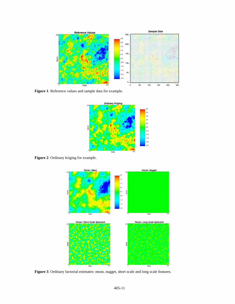
The first synthetic example is shown to show how factorial kriging approach works. A synthetic 256×256 2-D Gaussian variable was simulated with a small nugget effect (10%) and two isotropic spherical structures equally explaining the remaining 90% of the variability. The ranges of the spherical structures are 16 and 64 units. Data were sampled from the reference grid at a very close 5×5 spacing to produce sample data. The reference grid and sample data are shown on Figure 1.

As developed above, conventional factorial kriging is based on ordinary kriging. The sum of the estimate of each factor adds up to the ordinary kriging estimate. The ordinary kriging estimates are shown on Figure 2. Note that the ordinary kriging estimates are smoother than the reference values – a characteristic property of all kriging. Note also that the data are reproduced exactly, but with an apparent discontinuity because of the nugget effect.

The ordinary factorial kriging estimates the mean and each factor independently. In this example there are the mean and three factors to be estimated. Maps of the factors are shown on Figure 3. Although the nugget effect map looks constant, it is not. There is a discontinuity at each data point. Note that the estimate of the mean reflects the most variability because of the unbiasedness constraints which forces sum of weights to be 0 for the considered factor. Although the kriging equation and unbiasedness condition is right, it is unrealistic that estimated mean factor has the majority of variability. Furthermore, estimated long range structure is destructed as shown in Figure 3 and has low variability.

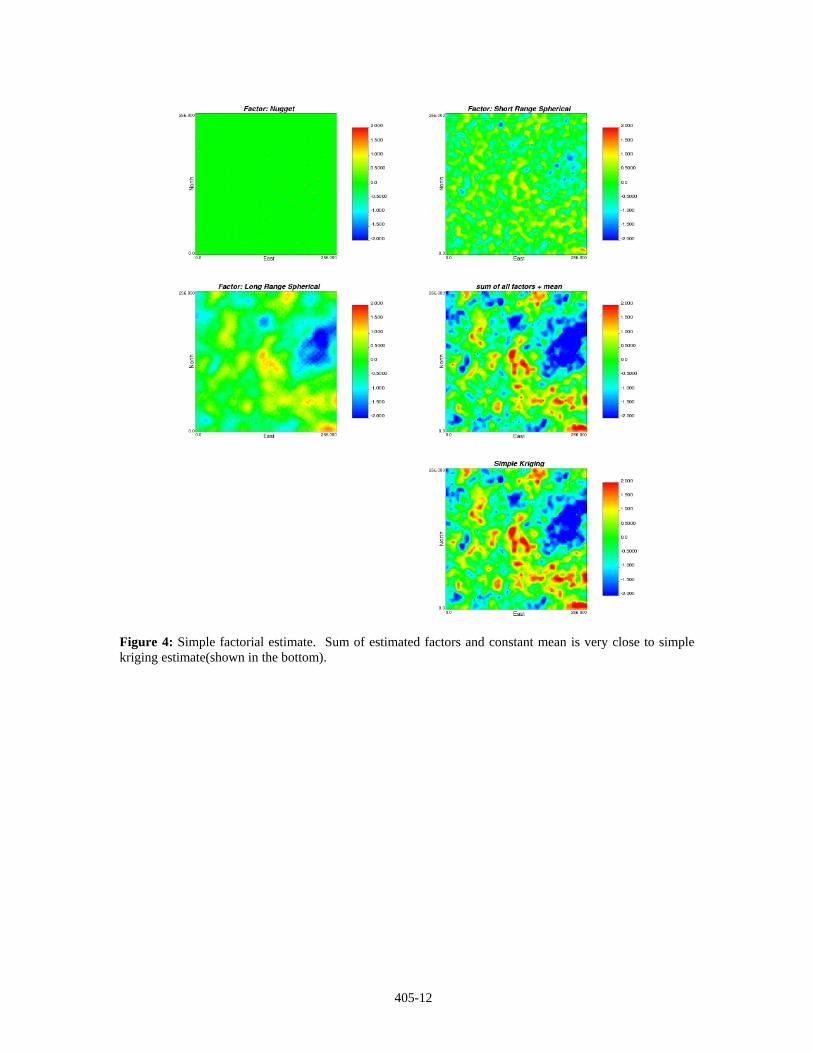
Simple factorial kriging estimates of each factor are shown in Figure 4. The mean value is assumed to be constant overall. Short range factor estimates have variability within short distance and long range factor estimates have variability within large distance in terms of visual interpretation. Simple factorial estimates reflect realistic features contrary to the ordinary factorial kriging estimates. Short range feature and long range features are identified significantly. Over every estimation location, sum of all estimated factors reproduced simple kriged value as we have theoretically derived equation (4).

OFK vs SFK

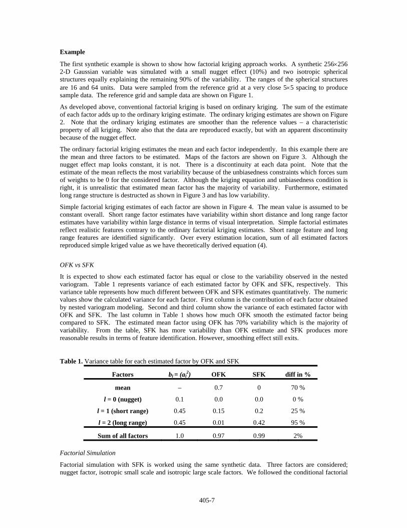
It is expected to show each estimated factor has equal or close to the variability observed in the nested variogram. Table 1 represents variance of each estimated factor by OFK and SFK, respectively. This variance table represents how much different between OFK and SFK estimates quantitatively. The numeric values show the calculated variance for each factor. First column is the contribution of each factor obtained by nested variogram modeling. Second and third column show the variance of each estimated factor with OFK and SFK. The last column in Table 1 shows how much OFK smooth the estimated factor being compared to SFK. The estimated mean factor using OFK has 70% variability which is the majority of variability. From the table, SFK has more variability than OFK estimate and SFK produces more reasonable results in terms of feature identification. However, smoothing effect still exits.

Table 1. Variance table for each estimated factor by OFK and SFK

Factors bl = (al2) OFK SFK diff in %

mean – 0.7 0 70 %

l = 0 (nugget) 0.1 0.0 0.0 0 %

l = 1 (short range) 0.45 0.15 0.2 25 %

l = 2 (long range) 0.45 0.01 0.42 95 %

Sum of all factors 1.0 0.97 0.99 2%

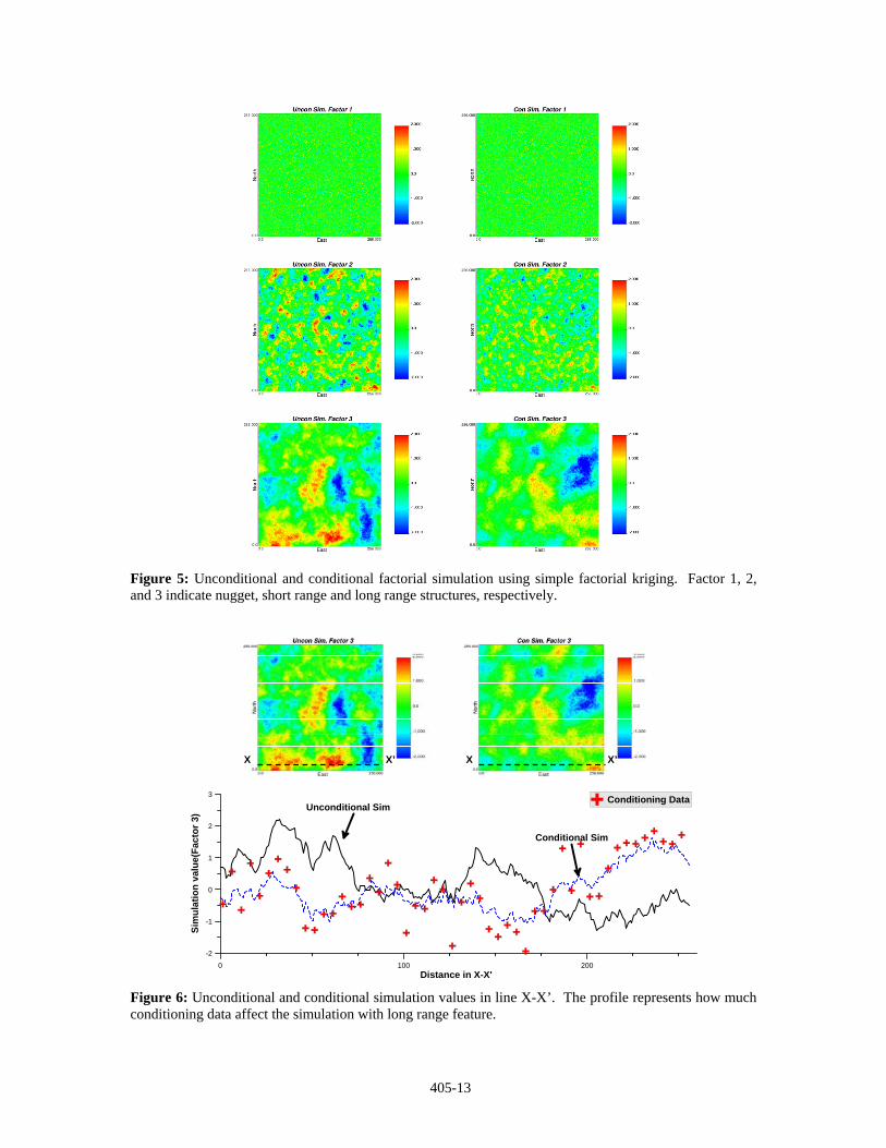
Factorial Simulation

Factorial simulation with SFK is worked using the same synthetic data. Three factors are considered; nugget factor, isotropic small scale and isotropic large scale factors. We followed the conditional factorial

405-8

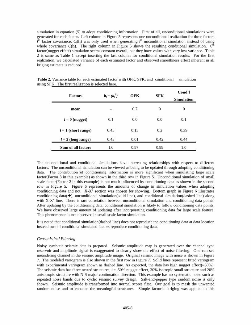
simulation in equation (5) to adopt conditioning information. First of all, unconditional simulations were generated for each factor. Left column in Figure 5 represents one unconditional realization for three factors. lth factor covariance, Cl(h) was only used when generating lth unconditional simulation instead of using whole covariance C(h). The right column in Figure 5 shows the resulting conditional simulation. 0th factor(nugget effect) simulation seems constant overall, but they have values with very low variance. Table 2 is same as Table 1 except inserting the last column for conditional simulation results. For the first realization, we calculated variance of each estimated factor and observed smoothness effect inherent in all kriging estimate is reduced.

Table 2. Variance table for each estimated factor with OFK, SFK, and conditional simulation using SFK. The first realization is selected here.

Factors bl = (al2) OFK SFK

Cond’l

Simulation

mean – 0.7 0 0

l = 0 (nugget) 0.1 0.0 0.0 0.1

l = 1 (short range) 0.45 0.15 0.2 0.39

l = 2 (long range) 0.45 0.01 0.42 0.44

Sum of all factors 1.0 0.97 0.99 1.0

The unconditional and conditional simulations have interesting relationships with respect to different factors. The unconditional simulation can be viewed as being to be updated through adopting conditioning data. The contribution of conditioning information is more significant when simulating large scale factor(Factor 3 in this example) as shown in the third row in Figure 5. Unconditional simulation of small scale factor(Factor 2 in this example) is not much influenced by conditioning data as shown in the second row in Figure 5. Figure 6 represents the amounts of change in simulation values when adopting conditioning data and not. X-X’ section was chosen for showing. Bottom graph in Figure 6 illustrates conditioning data( ), unconditional simulation(solid line), and conditional simulation(dashed line) along with X-X’ line. There is rare correlation between unconditional simulation and conditioning data points. After updating by the conditioning data, conditional simulation is likely to follow conditioning data points. We have observed large amount of updating after incorporating conditioning data for large scale feature. This phenomenon is not observed in small scale factor simulation.

It is noted that conditional simulation(dashed line) does not reproduce the conditioning data at data location instead sum of conditional simulated factors reproduce conditioning data.

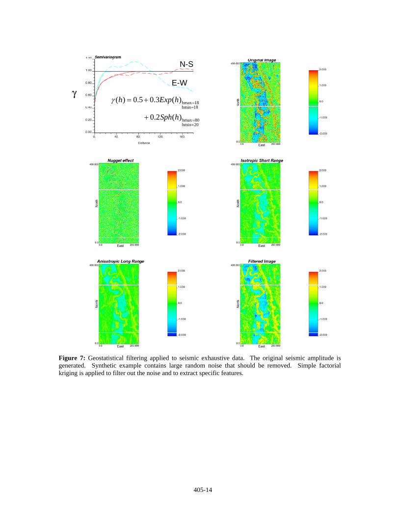
Geostatistical Filtering

Noisy synthetic seismic data is prepared. Seismic amplitude map is generated over the channel type reservoir and amplitude signal is exaggerated to clearly show the effect of noise filtering. One can see meandering channel in the seismic amplitude image. Original seismic image with noise is shown in Figure 7. The modeled variogram is also shown in the first row in Figure 7. Solid lines represent fitted variogram with experimental variogram shown as dashed line. As expected, the data has high nugget effect(≈50%). The seismic data has three nested structures, i.e. 50% nugget effect, 30% isotropic small structure and 20% anisotropic structure with N-S major continuation direction. This example has no systematic noise such as repeated noise bands due to cyclic seismic survey design. Salt-and-pepper type random noise is only shown. Seismic amplitude is transformed into normal scores first. Our goal is to mask the unwanted random noise and to enhance the meaningful structures. Simple factorial kriging was applied to this

405-9

example. Second and third row in Figure 7 show extracted factors corresponding to nugget, isotropic short range, and anisotropic long range. Nugget effect is due to random noise so that we filtered out nugget factor and resulting filtered image is shown in the lower right in the same figure. Random noise is largely removed with preserving small feature and large feature.

Geostatistical filtering is basically depending on the number and types of fitted variogram. This is one advantage of geostatistical filtering technique since geologic knowledge can be added when fitting the experimental variogram hence more realistic structure may be extracted.

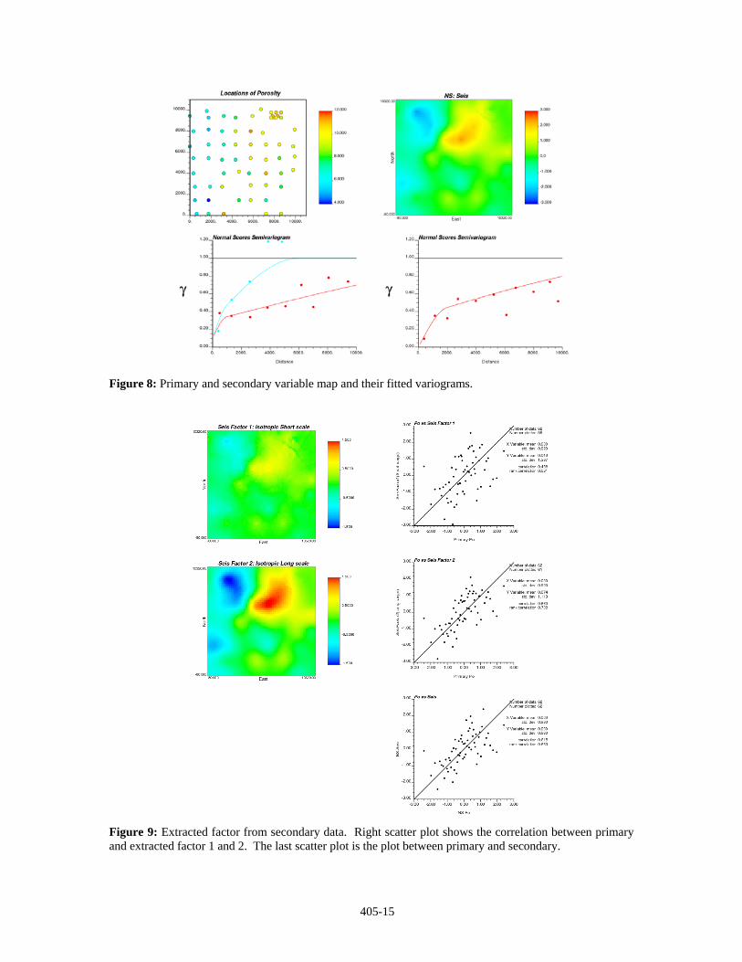
Data Integration

Amoco.dat data is considered for data integration. We have one primary porosity variable to be estimated and one exhaustively sampled seismic data. Location of primary porosity is shown in upper left of Figure 8. Normal score seismic amplitude is shown in right of the figure. Fitted variogram of porosity has three identified features, i.e. 10% nugget effect, 20% isotropic small scale and 70% anisotropic large scale features (major in N-S and minor in E-W).

hmin=hmax 1000 hmin=6000hmax=25000

( ) 0.1 0.2 ( ) 0.7 ( )Sph Sphγ == + +h h h

Seismic data appears to be varied smoothly. Variogram of secondary data is fitted as having two features, 35% isotropic small scale and 65% isotropic large scale features.

hmin=hmax 2000 hmin=hmax=20000( ) 0.35 ( ) 0.65 ( )Sph Sphγ == +h h h

First, simple factorial kriging with exhaustive seismic data was performed and two factors are extracted separately: isotropic small scaled feature and isotropic large scaled feature. Extracted factors are shown in Figure 9. To check the relationships between primary porosity and extracted factor, scatter plots are shown in the right column in Figure 9. Correlation of primary, Z(uα) and total seismic variable, Y(uα) is summarized as ρZY and ρZY is 0.615. It is noted that correlation coefficient is slightly changed when plotting extracted factor 1 and 2 with primary variable,

10.488 0.615

l totalZY ZYρ ρ== < =

20.660 0.615

l totalZY ZYρ ρ== > =

where Yl=1 is an extracted small scale feature and Yl=2 is an extracted large scale feature from original seismic data noted as Ytotal. We checked that large scale factor is more relevant feature to the primary variable. This is reasonable result since the variogram of primary porosity has greater contribution of large scale feature (70% variability) than small scale feature (20% variability). Besides, the variogram of seismic data shows 65% variability contribution of large scale feature. Although the difference between

1lZYρ=

and

totalZYρ or the difference between2lZYρ

= and

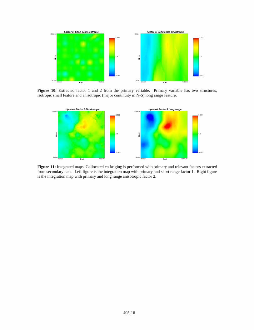
totalZYρ is not large, it is important to check that extracted relevant factor is more related to the primary variable to be estimated. Figure 11 represents the integrated isotropic small scale feature and anisotropic large scale feature using factorial collocated co-kriging equation (7). To identify isotropic small scale feature, primary variable and extracted isotropic small scale factor are co-kriged. To identify anisotropic large scale factor, primary variable and extracted isotropic large scale factor are co-kriged. All co-kriged estimates are shown in Figure 11.

To see how much update after integration, small scale and large scale features extracted only from primary porosity are plotted in Figure 10. Anisotropic long range structure is significant along with N-S direction. The variance of small scale factor is very low due to smoothness effect. Co-kriged factor 1 and 2 has more variability as shown in Figure 11.

405-10

Conclusions

An improved factorial kriging algorithm has been proposed to identify features. Conventional factorial kriging method has been reviewed and tested on synthetic example, and they showed unrealistic estimation even though kriging equation and constraint are theoretically right. An improved factorial kriging adopts simple kriging paradigm. Unknown mean is assumed to be constant overall and simple factorial kriging was applied on the example data. Features with different scale are identified well rather than using conventional factorial kriging.

Factorial simulation with simple factorial kriging has been suggested to correct smoothness of kriging. Conditional factorial simulation worked based on combination of factorial kriging and unconditional factorial simulation. Unconditional factorial simulation was updated significantly in large scale feature after assigning conditioning data. Factorial simulation corrects the kriging smoothness.

Other application of factorial kriging was to mask noise in exhaustive seismic data and to amplify the specific spatial features. Synthetic seismic amplitude data was prepared with large random noise. Simple factorial kriging successfully filtered out the unwanted random noise and enhanced the specific spatial factors. Factorial kriging approach makes it possible to integrate more relevant feature with primary variable. We have tested factorial collocated co-kriging using sparely sampled porosity and extracted relevant factor from seismic data. After integrating, we have identified spatial features with different scales which are hidden in the primary variable.

References

Chiles J-P. and Delfiner P., 1999, Geostatistics Modeling Spatial Uncertainty, John Wiley & Sons, Inc.

Deutsch, C.V. and Journel, A.G., 1998, GSLIB: Geostatistical Software Library: and User’s Guide. Oxford University Press, New York, 2nd Ed.

Goovaerts, P., 1997, Geostatistics for Natural Resources Evaluation, Oxford University Press, New York.

Deutsch, C.V., 2007 A Recall of Factorial Kriging with Examples and a Modified Version of kt3d, Centre for Computatinal Geostatistics Annual Report 9.

405-11

Figure 1: Reference values and sample data for example.

Figure 2: Ordinary kriging for example.

Figure 3: Ordinary factorial estimates: mean, nugget, short scale and long scale features.

405-12

Figure 4: Simple factorial estimate. Sum of estimated factors and constant mean is very close to simple kriging estimate(shown in the bottom).

405-13

Figure 5: Unconditional and conditional factorial simulation using simple factorial kriging. Factor 1, 2, and 3 indicate nugget, short range and long range structures, respectively.

X X’ X X’

0 100 200Distance in X-X'

-2

-1

0

1

2

3

Sim

ulat

ion

valu

e(Fa

ctor

3) Unconditional Sim

Conditional Sim

Conditioning Data

Figure 6: Unconditional and conditional simulation values in line X-X’. The profile represents how much conditioning data affect the simulation with long range feature.

405-14

N-S

E-W

hmax 18hmin 18

hmax 80hmin 20

( ) 0.5 0.3 ( )

0.2 ( )

h Exp h

Sph h

γ ==

==

= +

+

Figure 7: Geostatistical filtering applied to seismic exhaustive data. The original seismic amplitude is generated. Synthetic example contains large random noise that should be removed. Simple factorial kriging is applied to filter out the noise and to extract specific features.

405-15

Figure 8: Primary and secondary variable map and their fitted variograms.

Figure 9: Extracted factor from secondary data. Right scatter plot shows the correlation between primary and extracted factor 1 and 2. The last scatter plot is the plot between primary and secondary.

405-16

Figure 10: Extracted factor 1 and 2 from the primary variable. Primary variable has two structures, isotropic small feature and anisotropic (major continuity in N-S) long range feature.

Figure 11: Integrated maps. Collocated co-kriging is performed with primary and relevant factors extracted from secondary data. Left figure is the integration map with primary and short range factor 1. Right figure is the integration map with primary and long range anisotropic factor 2.