4 Vehicle operating costs

27

4 Vehicle operating costsVOC by definition are the costs associated with operating a motor vehicle. VOC are made up of fuel, oil, tyre, repairs and maintenance and interest and depreciation costs. The calculation of each component of VOC is based on a detailed methodology. The calculation of VOC is impacted by a number of inputs and adjustments are made accordingly.

4

4.28

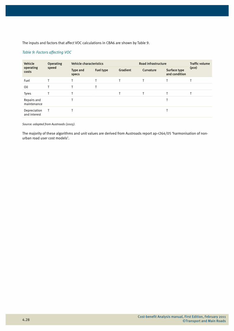
The inputs and factors that affect VOC calculations in CBA6 are shown by Table 9.

Table 9: Factors affecting VOC

Vehicle operating costs

Operating speed

Vehicle characteristics Road infrastructure Traffic volume (pce)

Type and specs

Fuel type Gradient Curvature Surface type and condition

Fuel T T T T T T T

Oil T T T

Tyres T T T T T T

Repairs and maintenance

T T

Depreciation and interest

T T T

Source: adapted from Austroads (2005).

The majority of these algorithms and unit values are derived from Austroads report ap-r264/05 ‘harmonisation of non-urban road user cost models’.

Cost-benefit Analysis manual, First Edition, February 2011 ©Transport and Main Roads

4.29

4.1 Fuel

Vehicle fuel cost is calculated based on the fuel consumption of each vehicle. Vehicle operating speed predominantly influences the rate of fuel consumption. Further adjustments to the rate of fuel consumption are made to account for site-specific details such as gradient, curvature, congestion and roughness.

4.1.1 Basic fuel consumption

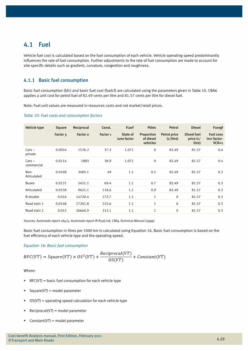
Basic fuel consumption (bfc) and basic fuel cost (fuelcf) are calculated using the parameters given in Table 10. CBA6 applies a unit cost for petrol fuel of 82.49 cents per litre and 81.57 cents per litre for diesel fuel.

Note: Fuel unit values are measured in resources costs and not market/retail prices.

Table 10: Fuel costs and consumption factors

Vehicle type Square Reciprocal Const. Fcavf Pdies Petrol Diesel Fcongf

Factor 3 Factor 2 Factor 1 State of tune factor

Proportion of diesel vehicles

Petrol price (c/litre)

Diesel fuel price (c/

litre)

Fuel cons incr factor-

VCR=1

Cars – private

0.0054 1526.2 37.3 1.071 0 82.49 81.57 0.4

Cars – commercial

0.0114 1883 38.9 1.071 0 82.49 81.57 0.4

Non-Articulated

0.0168 3485.1 49 1.1 0.5 82.49 81.57 0.3

Buses 0.0131 5451.1 69.4 1.1 0.7 82.49 81.57 0.3

Articulated 0.0158 9621.1 118.6 1.1 0.9 82.49 81.57 0.3

B-double 0.016 14720.4 172.7 1.1 1 0 81.57 0.3

Road train 1 0.0148 17201.8 223.6 1.1 1 0 81.57 0.3

Road train 2 0.015 26646.9 312.1 1.1 1 0 81.57 0.3

Sources: Austroads report 264/5, Austroads report IR-R156/08, CBA4 Technical Manual (1999).

Basic fuel consumption in litres per 1000 km is calculated using Equation 16. Basic fuel consumption is based on the fuel efficiency of each vehicle type and the operating speed.

Equation 16: Basic fuel consumption

Where:

• BFC(VT) = basic fuel consumption for each vehicle type

• Square(VT) = model parameter

• OS(VT) = operating speed calculation for each vehicle type

• Reciprocal(VT) = model parameter

• Constant(VT) = model parameter


4.30

Basic fuel consumption is a function of the default model parameters shown by Table 10. For a graphical representation of the relationship between variables, refer to Figure 12. At this early stage in the fuel consumption calculation, these values will not vary by project location.

Example: Basic fuel consumption

Basic fuel consumption in litres per 1000 km for a B-double with an operating speed of 64.4 km/h (as calculated in Section 3) is determined as follows:

This shows that at a constant speed of 64.4 km/h, a B-double will consume 467.5 litres of fuel for every 1000 km travelled.

The basic fuel consumption calculation excludes other project-specific factors that affect vehicle fuel consumption. This calculation merely sets the base level from which the actual fuel consumption rate can be determined. The actual fuel consumption in litres per 1000 km is calculated by applying a series of adjustments for gradient, curvature, congestion and roughness.

4.1.2 Fuel consumption gradient correction factors

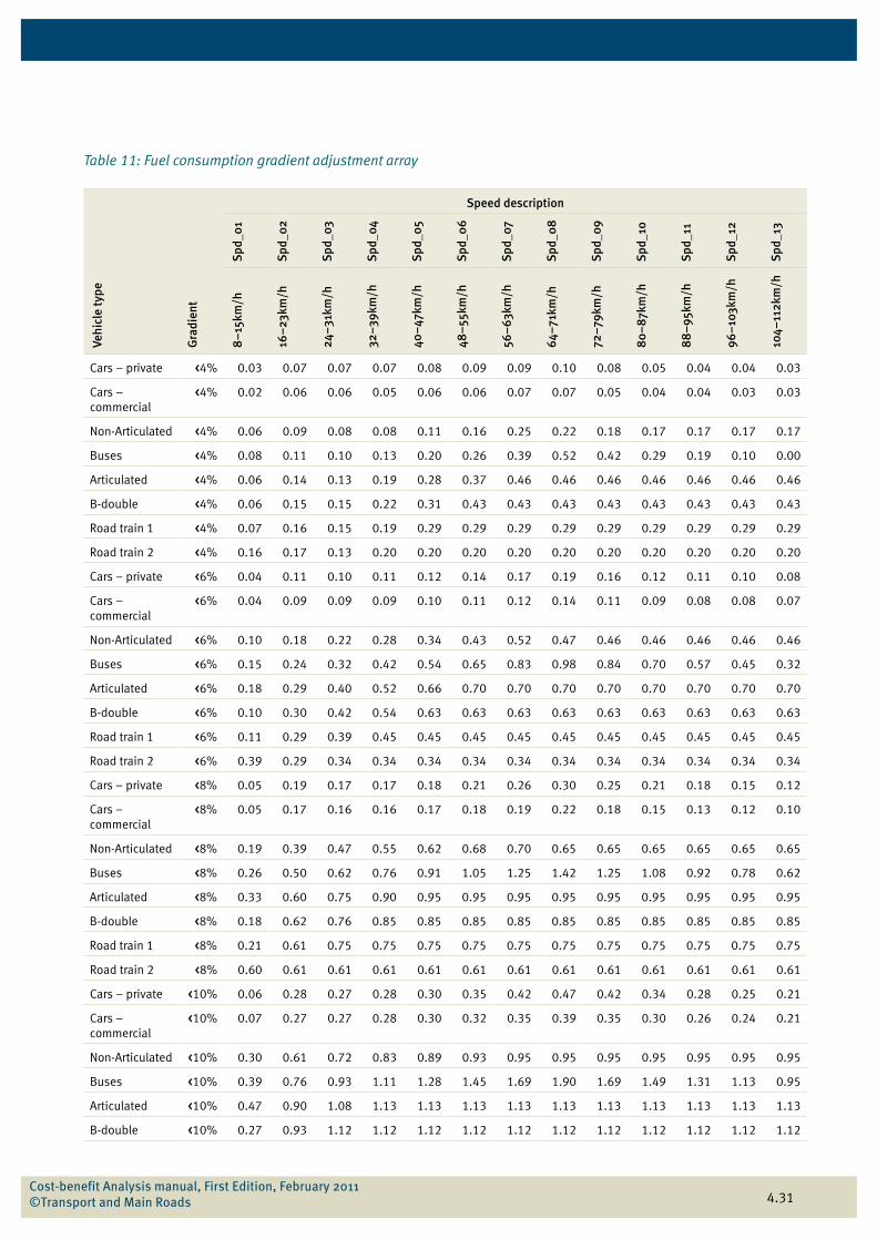
The gradient adjustment is calculated using the value obtained from the roughness and gradient correction factor values shown by Table 11. The adjustment is made to reflect increased fuel consumption due to a change in gradient. As gradients increase, the adjustment factor also increases, indicating a direct relationship. For example, the gradient adjustment of a private vehicle on a 10% gradient travelling at 40 km/h is 0.30. This indicates that fuel consumption is 30% higher than fuel consumption on a flat road with a grade of less than 4%.


4.31

Table 11: Fuel consumption gradient adjustment array

Vehi

cle

type

Gra

dien

tSpeed description

Spd

_01

Spd

_02

Spd

_03

Spd

_04

Spd

_05

Spd

_06

Spd

_07

Spd

_08

Spd

_09

Spd

_10

Spd

_11

Spd

_12

Spd

_13

8–

15km

/h

16–

23km

/h

24–

31km

/h

32–

39km

/h

40–

47km

/h

48–

55km

/h

56–

63km

/h

64–

71km

/h

72–

79km

/h

80–

87k

m/h

88

–95

km/h

96–

103k

m/h

104–

112k

m/h

Cars – private <4% 0.03 0.07 0.07 0.07 0.08 0.09 0.09 0.10 0.08 0.05 0.04 0.04 0.03

Cars – commercial

<4% 0.02 0.06 0.06 0.05 0.06 0.06 0.07 0.07 0.05 0.04 0.04 0.03 0.03

Non-Articulated <4% 0.06 0.09 0.08 0.08 0.11 0.16 0.25 0.22 0.18 0.17 0.17 0.17 0.17

Buses <4% 0.08 0.11 0.10 0.13 0.20 0.26 0.39 0.52 0.42 0.29 0.19 0.10 0.00

Articulated <4% 0.06 0.14 0.13 0.19 0.28 0.37 0.46 0.46 0.46 0.46 0.46 0.46 0.46

B-double <4% 0.06 0.15 0.15 0.22 0.31 0.43 0.43 0.43 0.43 0.43 0.43 0.43 0.43

Road train 1 <4% 0.07 0.16 0.15 0.19 0.29 0.29 0.29 0.29 0.29 0.29 0.29 0.29 0.29

Road train 2 <4% 0.16 0.17 0.13 0.20 0.20 0.20 0.20 0.20 0.20 0.20 0.20 0.20 0.20

Cars – private <6% 0.04 0.11 0.10 0.11 0.12 0.14 0.17 0.19 0.16 0.12 0.11 0.10 0.08

Cars – commercial

<6% 0.04 0.09 0.09 0.09 0.10 0.11 0.12 0.14 0.11 0.09 0.08 0.08 0.07

Non-Articulated <6% 0.10 0.18 0.22 0.28 0.34 0.43 0.52 0.47 0.46 0.46 0.46 0.46 0.46

Buses <6% 0.15 0.24 0.32 0.42 0.54 0.65 0.83 0.98 0.84 0.70 0.57 0.45 0.32

Articulated <6% 0.18 0.29 0.40 0.52 0.66 0.70 0.70 0.70 0.70 0.70 0.70 0.70 0.70

B-double <6% 0.10 0.30 0.42 0.54 0.63 0.63 0.63 0.63 0.63 0.63 0.63 0.63 0.63

Road train 1 <6% 0.11 0.29 0.39 0.45 0.45 0.45 0.45 0.45 0.45 0.45 0.45 0.45 0.45

Road train 2 <6% 0.39 0.29 0.34 0.34 0.34 0.34 0.34 0.34 0.34 0.34 0.34 0.34 0.34

Cars – private <8% 0.05 0.19 0.17 0.17 0.18 0.21 0.26 0.30 0.25 0.21 0.18 0.15 0.12

Cars – commercial

<8% 0.05 0.17 0.16 0.16 0.17 0.18 0.19 0.22 0.18 0.15 0.13 0.12 0.10

Non-Articulated <8% 0.19 0.39 0.47 0.55 0.62 0.68 0.70 0.65 0.65 0.65 0.65 0.65 0.65

Buses <8% 0.26 0.50 0.62 0.76 0.91 1.05 1.25 1.42 1.25 1.08 0.92 0.78 0.62

Articulated <8% 0.33 0.60 0.75 0.90 0.95 0.95 0.95 0.95 0.95 0.95 0.95 0.95 0.95

B-double <8% 0.18 0.62 0.76 0.85 0.85 0.85 0.85 0.85 0.85 0.85 0.85 0.85 0.85

Road train 1 <8% 0.21 0.61 0.75 0.75 0.75 0.75 0.75 0.75 0.75 0.75 0.75 0.75 0.75

Road train 2 <8% 0.60 0.61 0.61 0.61 0.61 0.61 0.61 0.61 0.61 0.61 0.61 0.61 0.61

Cars – private <10% 0.06 0.28 0.27 0.28 0.30 0.35 0.42 0.47 0.42 0.34 0.28 0.25 0.21

Cars – commercial

<10% 0.07 0.27 0.27 0.28 0.30 0.32 0.35 0.39 0.35 0.30 0.26 0.24 0.21

Non-Articulated <10% 0.30 0.61 0.72 0.83 0.89 0.93 0.95 0.95 0.95 0.95 0.95 0.95 0.95

Buses <10% 0.39 0.76 0.93 1.11 1.28 1.45 1.69 1.90 1.69 1.49 1.31 1.13 0.95

Articulated <10% 0.47 0.90 1.08 1.13 1.13 1.13 1.13 1.13 1.13 1.13 1.13 1.13 1.13

B-double <10% 0.27 0.93 1.12 1.12 1.12 1.12 1.12 1.12 1.12 1.12 1.12 1.12 1.12


4.32

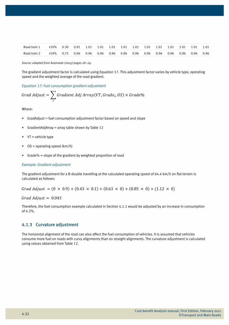
Road train 1 <10% 0.30 0.91 1.01 1.01 1.01 1.01 1.01 1.01 1.01 1.01 1.01 1.01 1.01

Road train 2 <10% 0.75 0.96 0.96 0.96 0.96 0.96 0.96 0.96 0.96 0.96 0.96 0.96 0.96

Source: adapted from Austroads (2005) pages 28–29.

The gradient adjustment factor is calculated using Equation 17. This adjustment factor varies by vehicle type, operating speed and the weighted average of the road gradient.

Equation 17: Fuel consumption gradient adjustment

Where:

• GradAdjust = fuel consumption adjustment factor based on speed and slope

• GradientAdjArray = array table shown by Table 12

• VT = vehicle type

• OS = operating speed (km/h)

• Grade% = slope of the gradient by weighted proportion of road

Example: Gradient adjustment

The gradient adjustment for a B-double travelling at the calculated operating speed of 64.4 km/h on flat terrain is calculated as follows:

Therefore, the fuel consumption example calculated in Section 4.1.1 would be adjusted by an increase in consumption of 4.3%.

4.1.3 Curvature adjustment

The horizontal alignment of the road can also affect the fuel consumption of vehicles. It is assumed that vehicles consume more fuel on roads with curvy alignments than on straight alignments. The curvature adjustment is calculated using values obtained from Table 12.


4.33

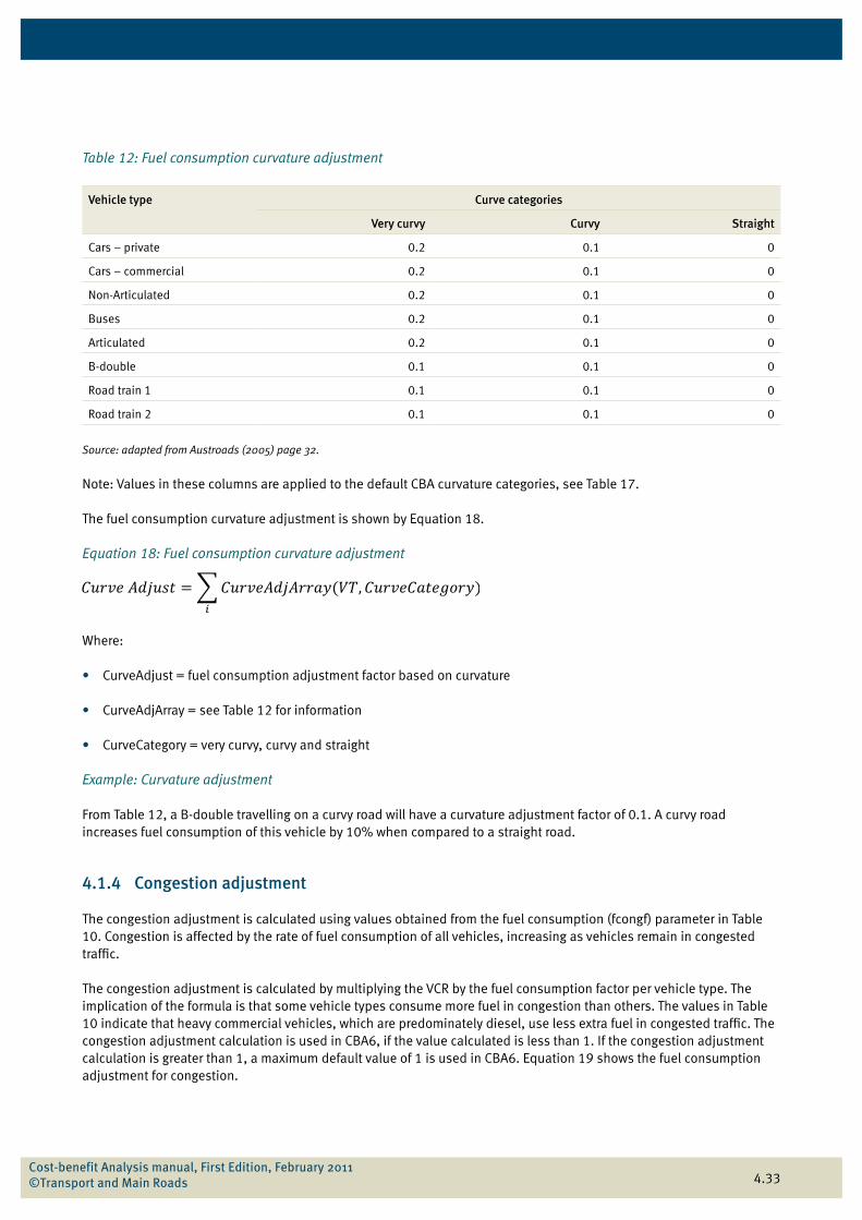
Table 12: Fuel consumption curvature adjustment

Vehicle type Curve categories

Very curvy Curvy Straight

Cars – private 0.2 0.1 0

Cars – commercial 0.2 0.1 0

Non-Articulated 0.2 0.1 0

Buses 0.2 0.1 0

Articulated 0.2 0.1 0

B-double 0.1 0.1 0

Road train 1 0.1 0.1 0

Road train 2 0.1 0.1 0

Source: adapted from Austroads (2005) page 32.

Note: Values in these columns are applied to the default CBA curvature categories, see Table 17.

The fuel consumption curvature adjustment is shown by Equation 18.

Equation 18: Fuel consumption curvature adjustment

Where:

• CurveAdjust = fuel consumption adjustment factor based on curvature

• CurveAdjArray = see Table 12 for information

• CurveCategory = very curvy, curvy and straight

Example: Curvature adjustment

From Table 12, a B-double travelling on a curvy road will have a curvature adjustment factor of 0.1. A curvy road increases fuel consumption of this vehicle by 10% when compared to a straight road.

4.1.4 Congestion adjustment

The congestion adjustment is calculated using values obtained from the fuel consumption (fcongf) parameter in Table 10. Congestion is affected by the rate of fuel consumption of all vehicles, increasing as vehicles remain in congested traffic.

The congestion adjustment is calculated by multiplying the VCR by the fuel consumption factor per vehicle type. The implication of the formula is that some vehicle types consume more fuel in congestion than others. The values in Table 10 indicate that heavy commercial vehicles, which are predominately diesel, use less extra fuel in congested traffic. The congestion adjustment calculation is used in CBA6, if the value calculated is less than 1. If the congestion adjustment calculation is greater than 1, a maximum default value of 1 is used in CBA6. Equation 19 shows the fuel consumption adjustment for congestion.


4.34

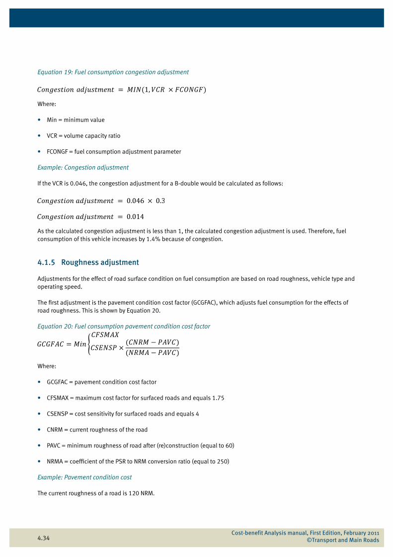
Equation 19: Fuel consumption congestion adjustment

Where:

• Min = minimum value

• VCR = volume capacity ratio

• FCONGF = fuel consumption adjustment parameter

Example: Congestion adjustment

If the VCR is 0.046, the congestion adjustment for a B-double would be calculated as follows:

As the calculated congestion adjustment is less than 1, the calculated congestion adjustment is used. Therefore, fuel consumption of this vehicle increases by 1.4% because of congestion.

4.1.5 Roughness adjustment

Adjustments for the effect of road surface condition on fuel consumption are based on road roughness, vehicle type and operating speed.

The first adjustment is the pavement condition cost factor (GCGFAC), which adjusts fuel consumption for the effects of road roughness. This is shown by Equation 20.

Equation 20: Fuel consumption pavement condition cost factor

Where:

• GCGFAC = pavement condition cost factor

• CFSMAX = maximum cost factor for surfaced roads and equals 1.75

• CSENSP = cost sensitivity for surfaced roads and equals 4

• CNRM = current roughness of the road

• PAVC = minimum roughness of road after (re)construction (equal to 60)

• NRMA = coefficient of the PSR to NRM conversion ratio (equal to 250)

Example: Pavement condition cost

The current roughness of a road is 120 NRM.


4.35

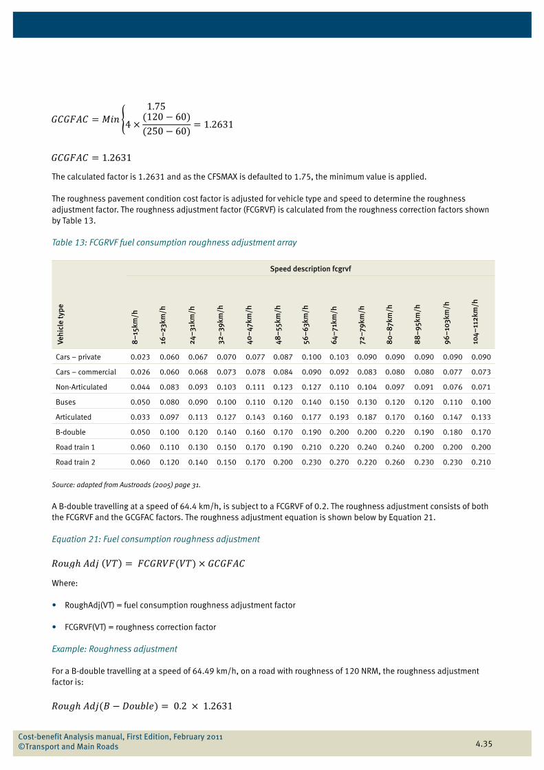
The calculated factor is 1.2631 and as the CFSMAX is defaulted to 1.75, the minimum value is applied.

The roughness pavement condition cost factor is adjusted for vehicle type and speed to determine the roughness adjustment factor. The roughness adjustment factor (FCGRVF) is calculated from the roughness correction factors shown by Table 13.

Table 13: FCGRVF fuel consumption roughness adjustment array

Vehi

cle

type

Speed description fcgrvf

8–

15km

/h

16–

23km

/h

24–

31km

/h

32–

39km

/h

40–

47km

/h

48–

55km

/h

56–

63km

/h

64–

71km

/h

72–

79km

/h

80–

87k

m/h

88

–95

km/h

96–

103k

m/h

104–

112k

m/h

Cars – private 0.023 0.060 0.067 0.070 0.077 0.087 0.100 0.103 0.090 0.090 0.090 0.090 0.090

Cars – commercial 0.026 0.060 0.068 0.073 0.078 0.084 0.090 0.092 0.083 0.080 0.080 0.077 0.073

Non-Articulated 0.044 0.083 0.093 0.103 0.111 0.123 0.127 0.110 0.104 0.097 0.091 0.076 0.071

Buses 0.050 0.080 0.090 0.100 0.110 0.120 0.140 0.150 0.130 0.120 0.120 0.110 0.100

Articulated 0.033 0.097 0.113 0.127 0.143 0.160 0.177 0.193 0.187 0.170 0.160 0.147 0.133

B-double 0.050 0.100 0.120 0.140 0.160 0.170 0.190 0.200 0.200 0.220 0.190 0.180 0.170

Road train 1 0.060 0.110 0.130 0.150 0.170 0.190 0.210 0.220 0.240 0.240 0.200 0.200 0.200

Road train 2 0.060 0.120 0.140 0.150 0.170 0.200 0.230 0.270 0.220 0.260 0.230 0.230 0.210


A B-double travelling at a speed of 64.4 km/h, is subject to a FCGRVF of 0.2. The roughness adjustment consists of both the FCGRVF and the GCGFAC factors. The roughness adjustment equation is shown below by Equation 21.

Equation 21: Fuel consumption roughness adjustment

Where:

• RoughAdj(VT) = fuel consumption roughness adjustment factor

• FCGRVF(VT) = roughness correction factor

Example: Roughness adjustment

For a B-double travelling at a speed of 64.49 km/h, on a road with roughness of 120 NRM, the roughness adjustment factor is:


4.36

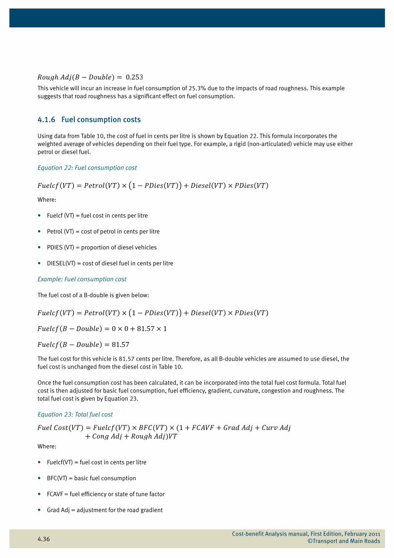
This vehicle will incur an increase in fuel consumption of 25.3% due to the impacts of road roughness. This example suggests that road roughness has a significant effect on fuel consumption.

4.1.6 Fuel consumption costs

Using data from Table 10, the cost of fuel in cents per litre is shown by Equation 22. This formula incorporates the weighted average of vehicles depending on their fuel type. For example, a rigid (non-articulated) vehicle may use either petrol or diesel fuel.

Equation 22: Fuel consumption cost

Where:

• Fuelcf (VT) = fuel cost in cents per litre

• Petrol (VT) = cost of petrol in cents per litre

• PDIES (VT) = proportion of diesel vehicles

• DIESEL(VT) = cost of diesel fuel in cents per litre

Example: Fuel consumption cost

The fuel cost of a B-double is given below:

The fuel cost for this vehicle is 81.57 cents per litre. Therefore, as all B-double vehicles are assumed to use diesel, the fuel cost is unchanged from the diesel cost in Table 10.

Once the fuel consumption cost has been calculated, it can be incorporated into the total fuel cost formula. Total fuel cost is then adjusted for basic fuel consumption, fuel efficiency, gradient, curvature, congestion and roughness. The total fuel cost is given by Equation 23.

Equation 23: Total fuel cost

Where:

• Fuelcf(VT) = fuel cost in cents per litre

• BFC(VT) = basic fuel consumption

• FCAVF = fuel efficiency or state of tune factor

• Grad Adj = adjustment for the road gradient


4.37

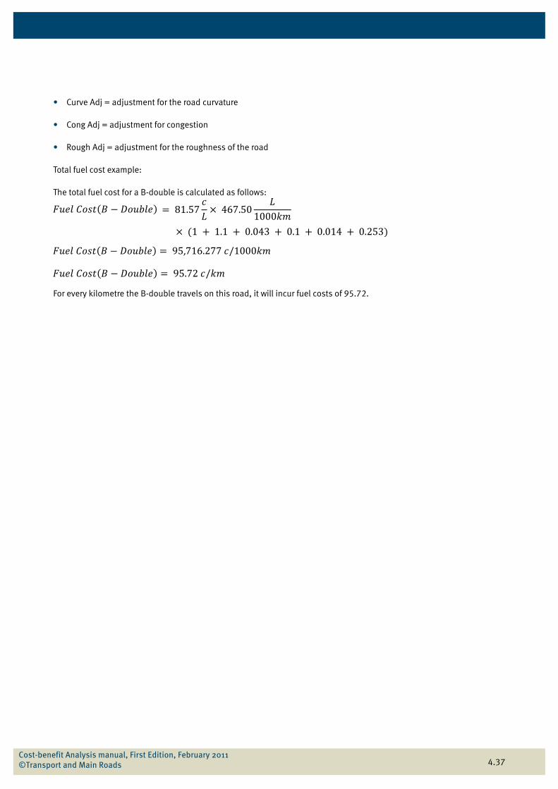
• Curve Adj = adjustment for the road curvature

• Cong Adj = adjustment for congestion

• Rough Adj = adjustment for the roughness of the road

Total fuel cost example:

The total fuel cost for a B-double is calculated as follows:

For every kilometre the B-double travels on this road, it will incur fuel costs of 95.72.


4.38

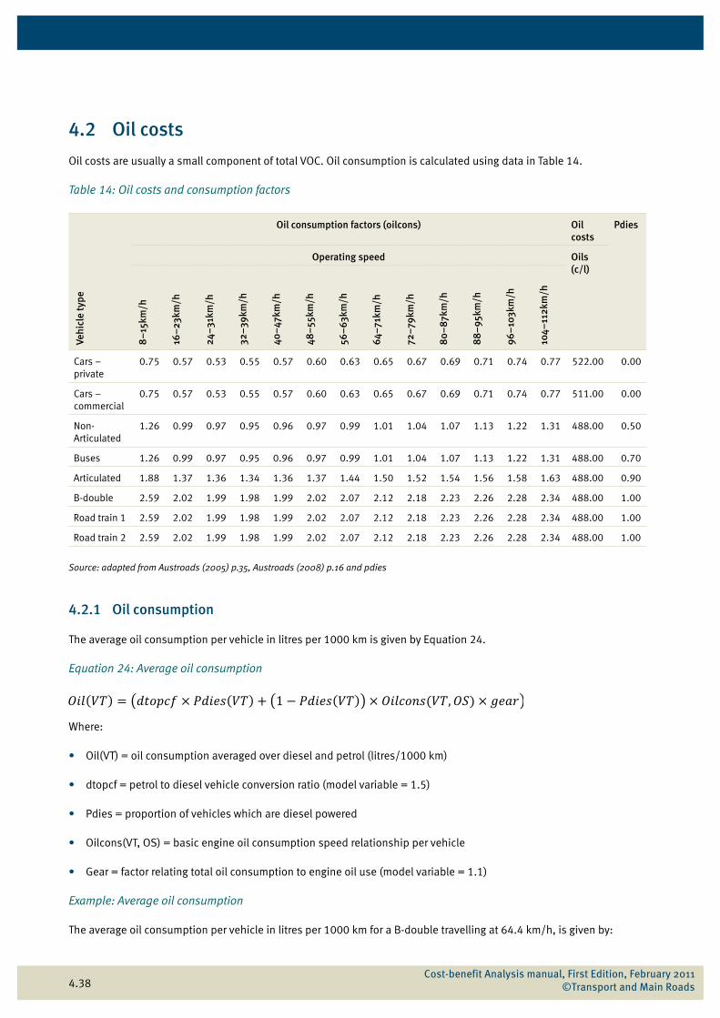
4.2 Oil costs

Oil costs are usually a small component of total VOC. Oil consumption is calculated using data in Table 14.

Table 14: Oil costs and consumption factors

Vehi

cle

type

Oil consumption factors (oilcons) Oil costs

Pdies

Operating speed Oils (c/l)

8–

15km

/h

16–

23km

/h

24–

31km

/h

32–

39km

/h

40–

47km

/h

48–

55km

/h

56–

63km

/h

64–

71km

/h

72–

79km

/h

80–

87k

m/h

88

–95

km/h

96–

103k

m/h

104–

112k

m/h

Cars – private

0.75 0.57 0.53 0.55 0.57 0.60 0.63 0.65 0.67 0.69 0.71 0.74 0.77 522.00 0.00

Cars – commercial

0.75 0.57 0.53 0.55 0.57 0.60 0.63 0.65 0.67 0.69 0.71 0.74 0.77 511.00 0.00

Non-Articulated

1.26 0.99 0.97 0.95 0.96 0.97 0.99 1.01 1.04 1.07 1.13 1.22 1.31 488.00 0.50

Buses 1.26 0.99 0.97 0.95 0.96 0.97 0.99 1.01 1.04 1.07 1.13 1.22 1.31 488.00 0.70

Articulated 1.88 1.37 1.36 1.34 1.36 1.37 1.44 1.50 1.52 1.54 1.56 1.58 1.63 488.00 0.90

B-double 2.59 2.02 1.99 1.98 1.99 2.02 2.07 2.12 2.18 2.23 2.26 2.28 2.34 488.00 1.00

Road train 1 2.59 2.02 1.99 1.98 1.99 2.02 2.07 2.12 2.18 2.23 2.26 2.28 2.34 488.00 1.00

Road train 2 2.59 2.02 1.99 1.98 1.99 2.02 2.07 2.12 2.18 2.23 2.26 2.28 2.34 488.00 1.00

Source: adapted from Austroads (2005) p.35, Austroads (2008) p.16 and pdies

4.2.1 Oil consumption

The average oil consumption per vehicle in litres per 1000 km is given by Equation 24.

Equation 24: Average oil consumption

Where:

• Oil(VT) = oil consumption averaged over diesel and petrol (litres/1000 km)

• dtopcf = petrol to diesel vehicle conversion ratio (model variable = 1.5)

• Pdies = proportion of vehicles which are diesel powered

• Oilcons(VT, OS) = basic engine oil consumption speed relationship per vehicle

• Gear = factor relating total oil consumption to engine oil use (model variable = 1.1)

Example: Average oil consumption

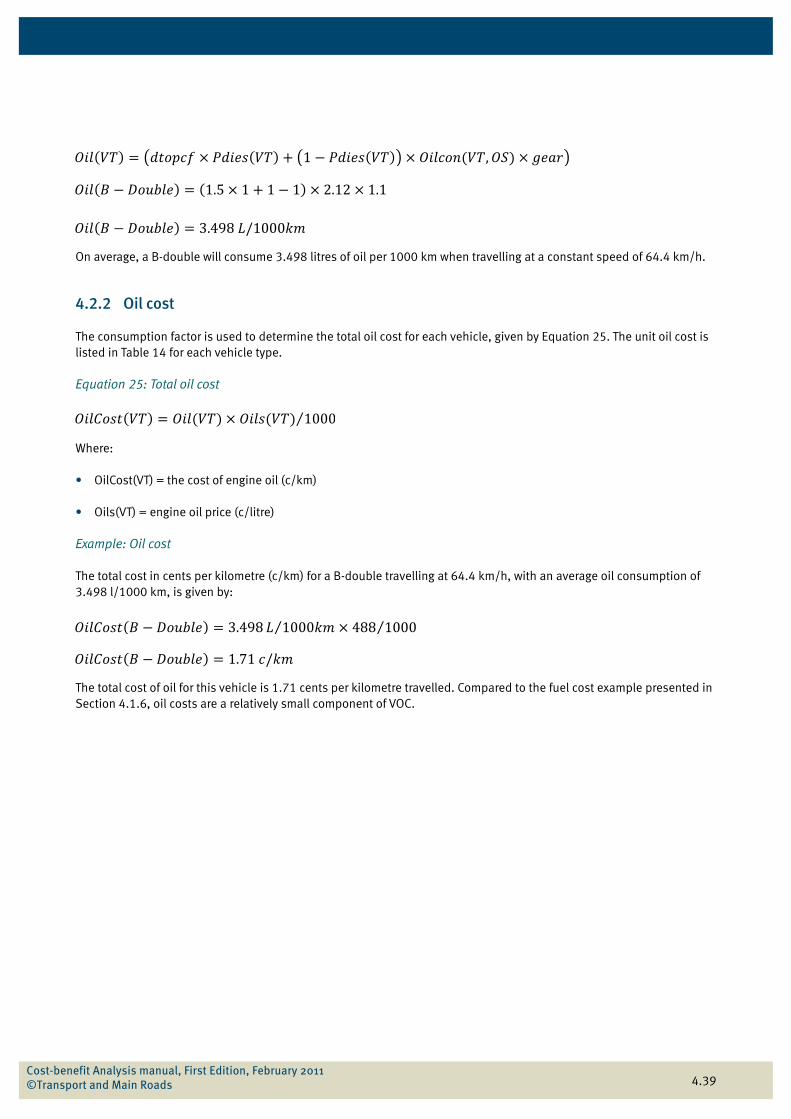
The average oil consumption per vehicle in litres per 1000 km for a B-double travelling at 64.4 km/h, is given by:


4.39

On average, a B-double will consume 3.498 litres of oil per 1000 km when travelling at a constant speed of 64.4 km/h.

4.2.2 Oil cost

The consumption factor is used to determine the total oil cost for each vehicle, given by Equation 25. The unit oil cost is listed in Table 14 for each vehicle type.

Equation 25: Total oil cost

Where:

• OilCost(VT) = the cost of engine oil (c/km)

• Oils(VT) = engine oil price (c/litre)

Example: Oil cost

The total cost in cents per kilometre (c/km) for a B-double travelling at 64.4 km/h, with an average oil consumption of 3.498 l/1000 km, is given by:

The total cost of oil for this vehicle is 1.71 cents per kilometre travelled. Compared to the fuel cost example presented in Section 4.1.6, oil costs are a relatively small component of VOC.

⁄


4.40

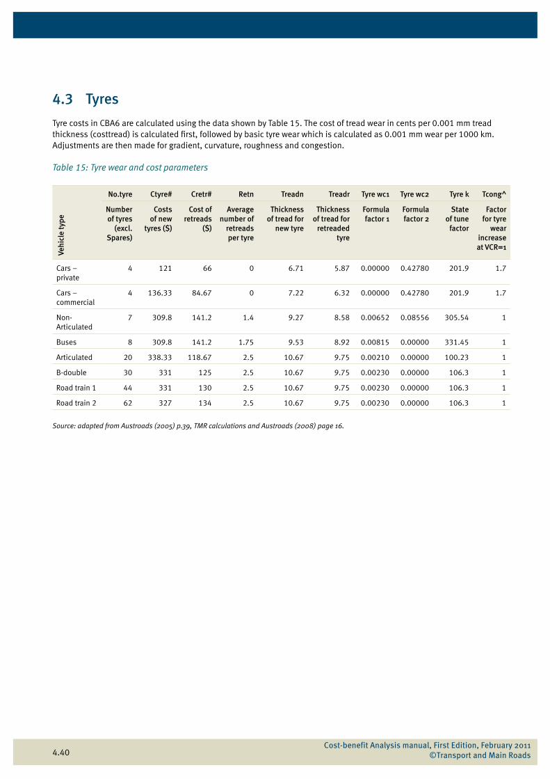
4.3 Tyres

Tyre costs in CBA6 are calculated using the data shown by Table 15. The cost of tread wear in cents per 0.001 mm tread thickness (costtread) is calculated first, followed by basic tyre wear which is calculated as 0.001 mm wear per 1000 km. Adjustments are then made for gradient, curvature, roughness and congestion.

Table 15: Tyre wear and cost parameters

Vehi

cle

type

No.tyre Ctyre# Cretr# Retn Treadn Treadr Tyre wc1 Tyre wc2 Tyre k Tcong^

Number of tyres

(excl. Spares)

Costs of new

tyres ($)

Cost of retreads

($)

Average number of

retreads per tyre

Thickness of tread for

new tyre

Thickness of tread for

retreaded tyre

Formula factor 1

Formula factor 2

State of tune

factor

Factor for tyre

wear increase at VCR=1

Cars – private

4 121 66 0 6.71 5.87 0.00000 0.42780 201.9 1.7

Cars – commercial

4 136.33 84.67 0 7.22 6.32 0.00000 0.42780 201.9 1.7

Non-Articulated

7 309.8 141.2 1.4 9.27 8.58 0.00652 0.08556 305.54 1

Buses 8 309.8 141.2 1.75 9.53 8.92 0.00815 0.00000 331.45 1

Articulated 20 338.33 118.67 2.5 10.67 9.75 0.00210 0.00000 100.23 1

B-double 30 331 125 2.5 10.67 9.75 0.00230 0.00000 106.3 1

Road train 1 44 331 130 2.5 10.67 9.75 0.00230 0.00000 106.3 1

Road train 2 62 327 134 2.5 10.67 9.75 0.00230 0.00000 106.3 1

Source: adapted from Austroads (2005) p.39, TMR calculations and Austroads (2008) page 16.


4.41

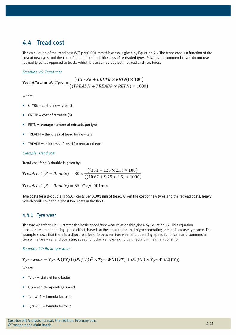
4.4 Tread cost

The calculation of the tread cost (VT) per 0.001 mm thickness is given by Equation 26. The tread cost is a function of the cost of new tyres and the cost of the number and thickness of retreaded tyres. Private and commercial cars do not use retread tyres, as opposed to trucks which it is assumed use both retread and new tyres.

Equation 26: Tread cost

Where:

• CTYRE = cost of new tyres ($)

• CRETR = cost of retreads ($)

• RETN = average number of retreads per tyre

• TREADN = thickness of tread for new tyre

• TREADR = thickness of tread for retreaded tyre

Example: Tread cost

Tread cost for a B-double is given by:

Tyre costs for a B-double is 55.07 cents per 0.001 mm of tread. Given the cost of new tyres and the retread costs, heavy vehicles will have the highest tyre costs in the fleet.

4.4.1 Tyre wear

The tyre wear formula illustrates the basic speed/tyre wear relationship given by Equation 27. This equation incorporates the operating speed effect, based on the assumption that higher operating speeds increase tyre wear. The example shows that there is a direct relationship between tyre wear and operating speed for private and commercial cars while tyre wear and operating speed for other vehicles exhibit a direct non-linear relationship.

Equation 27: Basic tyre wear

Where:

• Tyrek = state of tune factor

• OS = vehicle operating speed

• TyreWC1 = formula factor 1

• TyreWC2 = formula factor 2


4.42

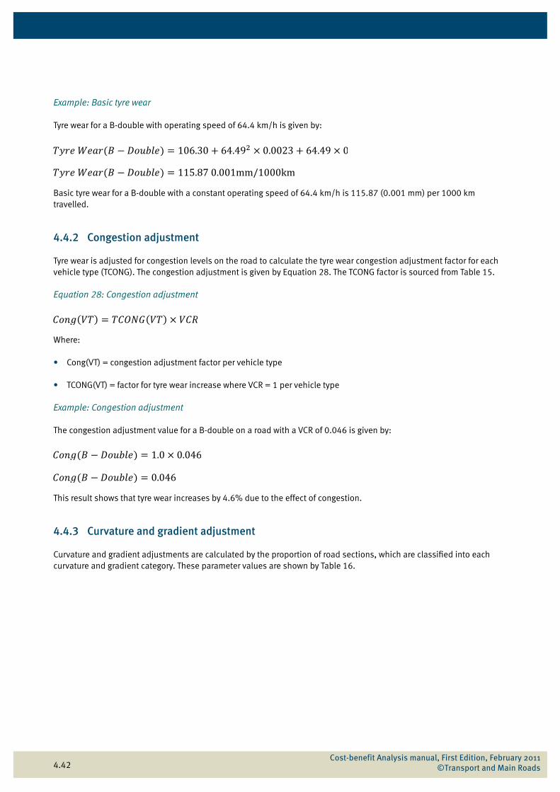
Example: Basic tyre wear

Tyre wear for a B-double with operating speed of 64.4 km/h is given by:

Basic tyre wear for a B-double with a constant operating speed of 64.4 km/h is 115.87 (0.001 mm) per 1000 km travelled.

4.4.2 Congestion adjustment

Tyre wear is adjusted for congestion levels on the road to calculate the tyre wear congestion adjustment factor for each vehicle type (TCONG). The congestion adjustment is given by Equation 28. The TCONG factor is sourced from Table 15.

Equation 28: Congestion adjustment

Where:

• Cong(VT) = congestion adjustment factor per vehicle type

• TCONG(VT) = factor for tyre wear increase where VCR = 1 per vehicle type

Example: Congestion adjustment

The congestion adjustment value for a B-double on a road with a VCR of 0.046 is given by:

This result shows that tyre wear increases by 4.6% due to the effect of congestion.

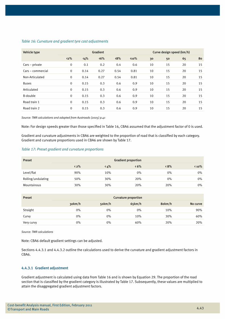
4.4.3 Curvature and gradient adjustment

Curvature and gradient adjustments are calculated by the proportion of road sections, which are classified into each curvature and gradient category. These parameter values are shown by Table 16.


4.43

Table 16: Curvature and gradient tyre cost adjustments

Vehicle type Gradient Curve design speed (km/h)

<2% <4% <6% <8% <10% 30 50 65 80

Cars – private 0 0.1 0.2 0.4 0.6 10 15 20 15

Cars – commercial 0 0.14 0.27 0.54 0.81 10 15 20 15

Non-Articulated 0 0.14 0.27 0.54 0.81 10 15 20 15

Buses 0 0.15 0.3 0.6 0.9 10 15 20 15

Articulated 0 0.15 0.3 0.6 0.9 10 15 20 15

B-double 0 0.15 0.3 0.6 0.9 10 15 20 15

Road train 1 0 0.15 0.3 0.6 0.9 10 15 20 15

Road train 2 0 0.15 0.3 0.6 0.9 10 15 20 15

Source: TMR calculations and adapted from Austroads (2005) p.41

Note: For design speeds greater than those specified in Table 16, CBA6 assumed that the adjustment factor of 0 is used.

Gradient and curvature adjustments in CBA6 are weighted to the proportion of road that is classified by each category. Gradient and curvature proportions used in CBA6 are shown by Table 17.

Table 17: Preset gradient and curvature proportions

Preset Gradient proportion

< 2% < 4% < 6% < 8% < 10%

Level/flat 90% 10% 0% 0% 0%

Rolling/undulating 50% 30% 20% 0% 0%

Mountainous 30% 30% 20% 20% 0%

Preset Curvature proportion

30km/h 50km/h 65km/h 80km/h No curve

Straight 0% 0% 0% 10% 90%

Curvy 0% 0% 10% 30% 60%

Very curvy 0% 0% 60% 20% 20%

Source: TMR calculations

Note: CBA6 default gradient settings can be adjusted.

Sections 4.4.3.1 and 4.4.3.2 outline the calculations used to derive the curvature and gradient adjustment factors in CBA6.

4.4.3.1 Gradient adjustment

Gradient adjustment is calculated using data from Table 16 and is shown by Equation 29. The proportion of the road section that is classified by the gradient category is illustrated by Table 17. Subsequently, these values are multiplied to attain the disaggregated gradient adjustment factors.


4.44

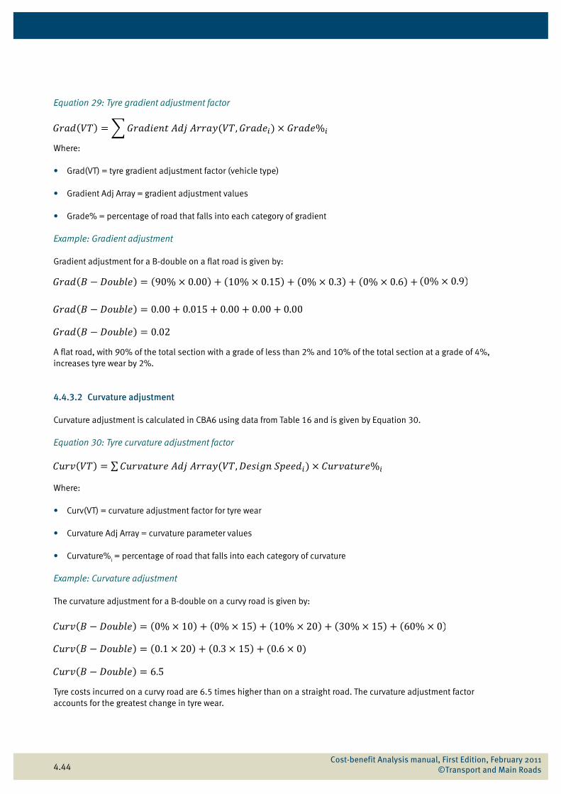
Equation 29: Tyre gradient adjustment factor

Where:

• Grad(VT) = tyre gradient adjustment factor (vehicle type)

• Gradient Adj Array = gradient adjustment values

• Grade% = percentage of road that falls into each category of gradient

Example: Gradient adjustment

Gradient adjustment for a B-double on a flat road is given by:

A flat road, with 90% of the total section with a grade of less than 2% and 10% of the total section at a grade of 4%, increases tyre wear by 2%.

4.4.3.2 Curvature adjustment

Curvature adjustment is calculated in CBA6 using data from Table 16 and is given by Equation 30.

Equation 30: Tyre curvature adjustment factor

Where:

• Curv(VT) = curvature adjustment factor for tyre wear

• Curvature Adj Array = curvature parameter values

• Curvature%i = percentage of road that falls into each category of curvature

Example: Curvature adjustment

The curvature adjustment for a B-double on a curvy road is given by:

Tyre costs incurred on a curvy road are 6.5 times higher than on a straight road. The curvature adjustment factor accounts for the greatest change in tyre wear.

∑


4.45

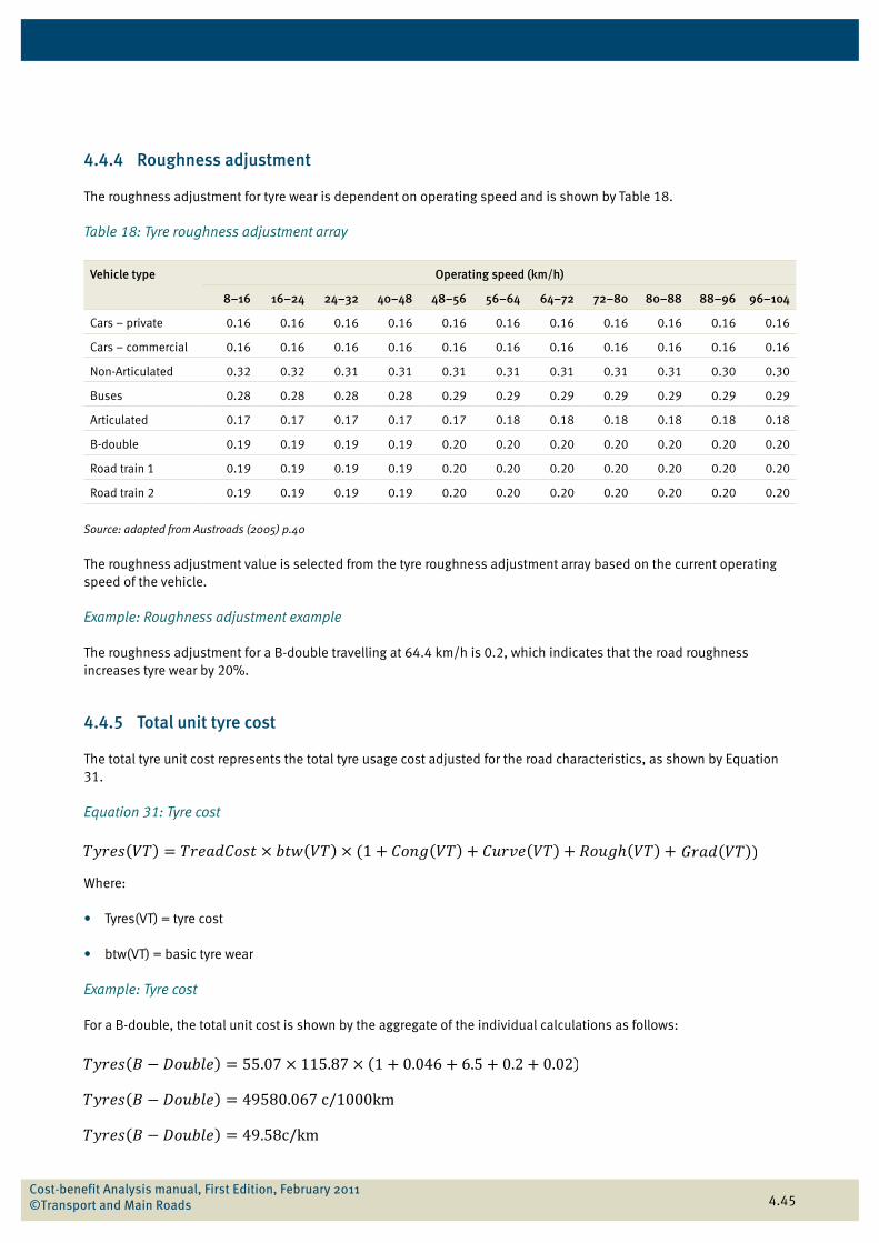
4.4.4 Roughness adjustment

The roughness adjustment for tyre wear is dependent on operating speed and is shown by Table 18.

Table 18: Tyre roughness adjustment array

Vehicle type Operating speed (km/h)

8–16 16–24 24–32 40–48 48–56 56–64 64–72 72–80 80–88 88–96 96–104

Cars – private 0.16 0.16 0.16 0.16 0.16 0.16 0.16 0.16 0.16 0.16 0.16

Cars – commercial 0.16 0.16 0.16 0.16 0.16 0.16 0.16 0.16 0.16 0.16 0.16

Non-Articulated 0.32 0.32 0.31 0.31 0.31 0.31 0.31 0.31 0.31 0.30 0.30

Buses 0.28 0.28 0.28 0.28 0.29 0.29 0.29 0.29 0.29 0.29 0.29

Articulated 0.17 0.17 0.17 0.17 0.17 0.18 0.18 0.18 0.18 0.18 0.18

B-double 0.19 0.19 0.19 0.19 0.20 0.20 0.20 0.20 0.20 0.20 0.20

Road train 1 0.19 0.19 0.19 0.19 0.20 0.20 0.20 0.20 0.20 0.20 0.20

Road train 2 0.19 0.19 0.19 0.19 0.20 0.20 0.20 0.20 0.20 0.20 0.20

Source: adapted from Austroads (2005) p.40

The roughness adjustment value is selected from the tyre roughness adjustment array based on the current operating speed of the vehicle.

Example: Roughness adjustment example

The roughness adjustment for a B-double travelling at 64.4 km/h is 0.2, which indicates that the road roughness increases tyre wear by 20%.

4.4.5 Total unit tyre cost

The total tyre unit cost represents the total tyre usage cost adjusted for the road characteristics, as shown by Equation 31.

Equation 31: Tyre cost

Where:

• Tyres(VT) = tyre cost

• btw(VT) = basic tyre wear

Example: Tyre cost

For a B-double, the total unit cost is shown by the aggregate of the individual calculations as follows:


4.46Cost-benefit Analysis manual, First Edition, February 2011

©Transport and Main Roads

4.47

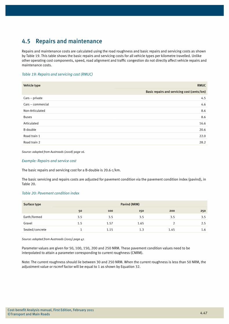
4.5 Repairs and maintenance

Repairs and maintenance costs are calculated using the road roughness and basic repairs and servicing costs as shown by Table 19. This table shows the basic repairs and servicing costs for all vehicle types per kilometre travelled. Unlike other operating cost components, speed, road alignment and traffic congestion do not directly affect vehicle repairs and maintenance costs.

Table 19: Repairs and servicing cost (RMUC)

Vehicle type RMUC

Basic repairs and servicing cost (cents/km)

Cars – private 4.5

Cars – commercial 4.6

Non-Articulated 8.6

Buses 8.6

Articulated 16.6

B-double 20.6

Road train 1 22.0

Road train 2 28.2


Example: Repairs and service cost

The basic repairs and servicing cost for a B-double is 20.6 c/km.

The basic servicing and repairs costs are adjusted for pavement condition via the pavement condition index (pavind), in Table 20.

Table 20: Pavement condition index

Surface type Pavind (NRM)

50 100 150 200 250

Earth/formed 3.5 3.5 3.5 3.5 3.5

Gravel 1.5 1.57 1.65 2 2.5

Sealed/concrete 1 1.15 1.3 1.45 1.6


Parameter values are given for 50, 100, 150, 200 and 250 NRM. These pavement condition values need to be interpolated to attain a parameter corresponding to current roughness (CNRM).

Note: The current roughness should lie between 30 and 250 NRM. When the current roughness is less than 50 NRM, the adjustment value or rscmrf factor will be equal to 1 as shown by Equation 32.


4.48

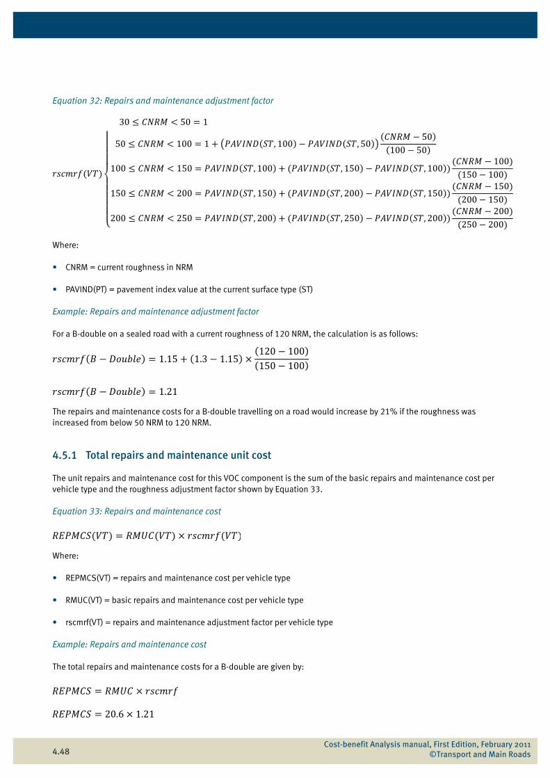
Equation 32: Repairs and maintenance adjustment factor

Where:

• CNRM = current roughness in NRM

• PAVIND(PT) = pavement index value at the current surface type (ST)

Example: Repairs and maintenance adjustment factor

For a B-double on a sealed road with a current roughness of 120 NRM, the calculation is as follows:

The repairs and maintenance costs for a B-double travelling on a road would increase by 21% if the roughness was increased from below 50 NRM to 120 NRM.

4.5.1 Total repairs and maintenance unit cost

The unit repairs and maintenance cost for this VOC component is the sum of the basic repairs and maintenance cost per vehicle type and the roughness adjustment factor shown by Equation 33.

Equation 33: Repairs and maintenance cost

Where:

• REPMCS(VT) = repairs and maintenance cost per vehicle type

• RMUC(VT) = basic repairs and maintenance cost per vehicle type

• rscmrf(VT) = repairs and maintenance adjustment factor per vehicle type

Example: Repairs and maintenance cost

The total repairs and maintenance costs for a B-double are given by:


4.49

The repairs and maintenance costs for a B-double travelling on a 120 NRM road surface would incur a repairs and maintenance cost of 24.93 cents per kilometre travelled.


4.50

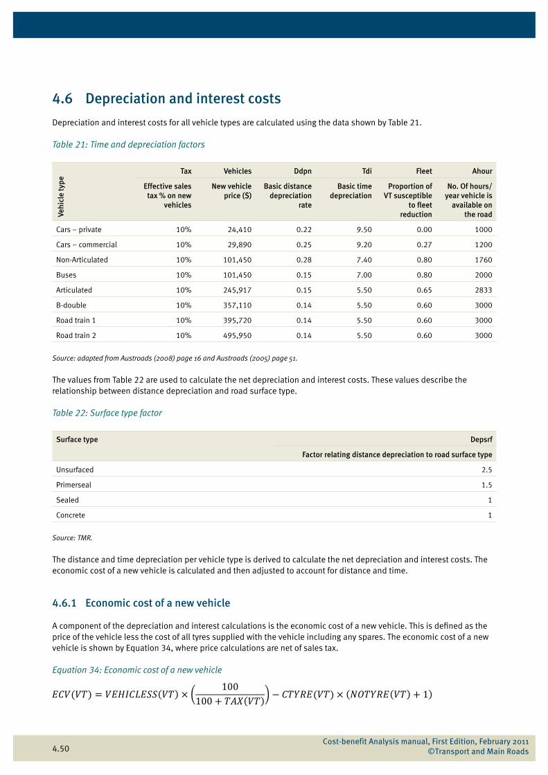
4.6 Depreciation and interest costs

Depreciation and interest costs for all vehicle types are calculated using the data shown by Table 21.

Table 21: Time and depreciation factors

Vehi

cle

type

Tax Vehicles Ddpn Tdi Fleet Ahour

Effective sales tax % on new

vehicles

New vehicle price ($)

Basic distance depreciation

rate

Basic time depreciation

Proportion of VT susceptible

to fleet reduction

No. Of hours/year vehicle is

available on the road

Cars – private 10% 24,410 0.22 9.50 0.00 1000

Cars – commercial 10% 29,890 0.25 9.20 0.27 1200

Non-Articulated 10% 101,450 0.28 7.40 0.80 1760

Buses 10% 101,450 0.15 7.00 0.80 2000

Articulated 10% 245,917 0.15 5.50 0.65 2833

B-double 10% 357,110 0.14 5.50 0.60 3000

Road train 1 10% 395,720 0.14 5.50 0.60 3000

Road train 2 10% 495,950 0.14 5.50 0.60 3000

Source: adapted from Austroads (2008) page 16 and Austroads (2005) page 51.

The values from Table 22 are used to calculate the net depreciation and interest costs. These values describe the relationship between distance depreciation and road surface type.

Table 22: Surface type factor

Surface type Depsrf

Factor relating distance depreciation to road surface type

Unsurfaced 2.5

Primerseal 1.5

Sealed 1

Concrete 1

Source: TMR.

The distance and time depreciation per vehicle type is derived to calculate the net depreciation and interest costs. The economic cost of a new vehicle is calculated and then adjusted to account for distance and time.

4.6.1 Economic cost of a new vehicle

A component of the depreciation and interest calculations is the economic cost of a new vehicle. This is defined as the price of the vehicle less the cost of all tyres supplied with the vehicle including any spares. The economic cost of a new vehicle is shown by Equation 34, where price calculations are net of sales tax.

Equation 34: Economic cost of a new vehicle

100


4.51

Where:

• ECV(VT) = economic cost of the vehicle

• VEHICLESS(VT) = new vehicle price per vehicle type ($)

• TAX = effective sales tax on new vehicles

• NOTYRE(VT) = number of tyres (including spares)

• CTYRE(VT) = cost of new tyres ($)

Example: Economic cost of a new vehicle

For a B-double , the economic cost of a new vehicle is:

The economic cost of a new B-double including sales tax and the number of tyres is $346 492.

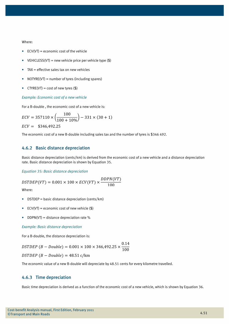
4.6.2 Basic distance depreciation

Basic distance depreciation (cents/km) is derived from the economic cost of a new vehicle and a distance depreciation rate. Basic distance depreciation is shown by Equation 35.

Equation 35: Basic distance depreciation

Where:

• DSTDEP = basic distance depreciation (cents/km)

• ECV(VT) = economic cost of new vehicle ($)

• DDPN(VT) = distance depreciation rate %

Example: Basic distance depreciation

For a B-double, the distance depreciation is:

The economic value of a new B-double will depreciate by 48.51 cents for every kilometre travelled.

4.6.3 Time depreciation

Basic time depreciation is derived as a function of the economic cost of a new vehicle, which is shown by Equation 36.


4.52

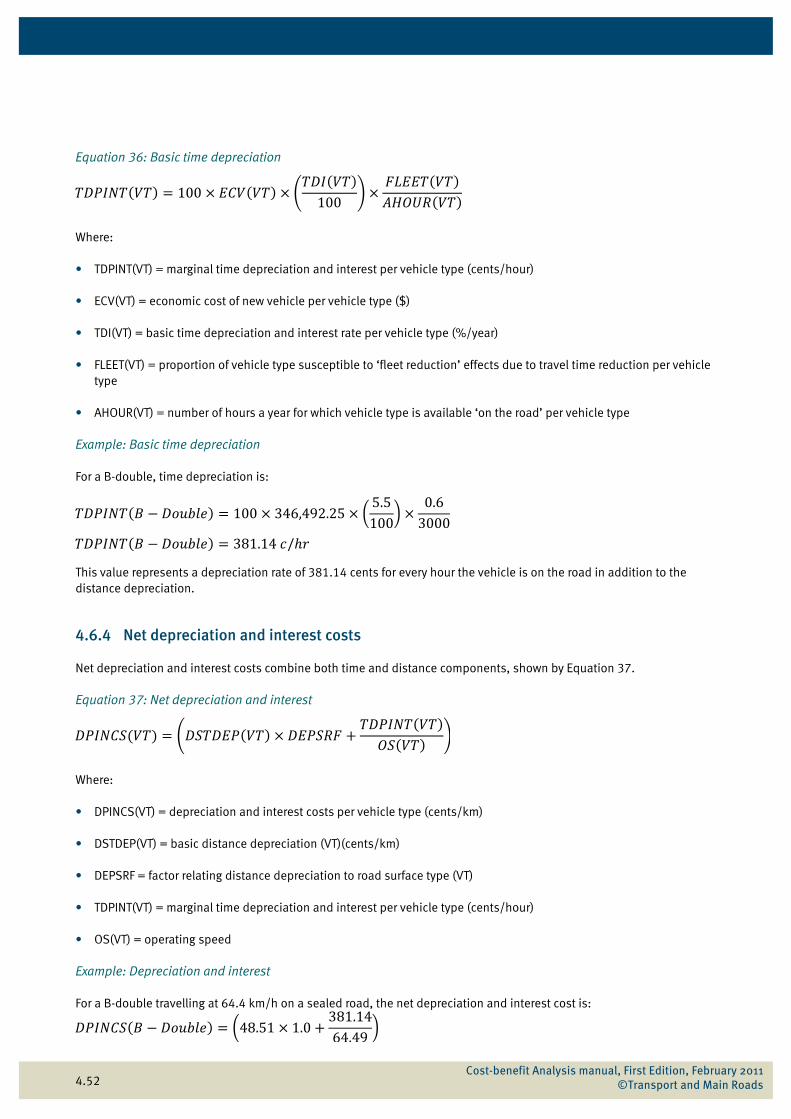
Equation 36: Basic time depreciation

Where:

• TDPINT(VT) = marginal time depreciation and interest per vehicle type (cents/hour)

• ECV(VT) = economic cost of new vehicle per vehicle type ($)

• TDI(VT) = basic time depreciation and interest rate per vehicle type (%/year)

• FLEET(VT) = proportion of vehicle type susceptible to ‘fleet reduction’ effects due to travel time reduction per vehicle type

• AHOUR(VT) = number of hours a year for which vehicle type is available ‘on the road’ per vehicle type

Example: Basic time depreciation

For a B-double, time depreciation is:

This value represents a depreciation rate of 381.14 cents for every hour the vehicle is on the road in addition to the distance depreciation.

4.6.4 Net depreciation and interest costs

Net depreciation and interest costs combine both time and distance components, shown by Equation 37.

Equation 37: Net depreciation and interest

Where:

• DPINCS(VT) = depreciation and interest costs per vehicle type (cents/km)

• DSTDEP(VT) = basic distance depreciation (VT)(cents/km)

• DEPSRF = factor relating distance depreciation to road surface type (VT)

• TDPINT(VT) = marginal time depreciation and interest per vehicle type (cents/hour)

• OS(VT) = operating speed

Example: Depreciation and interest

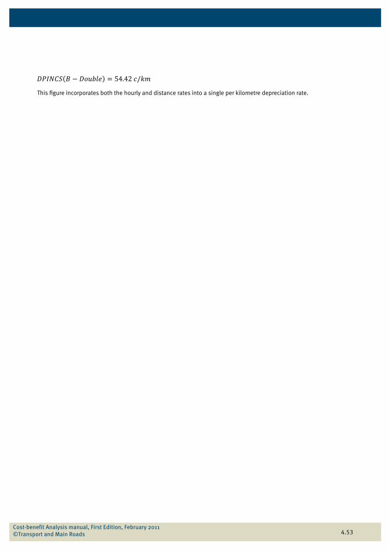
For a B-double travelling at 64.4 km/h on a sealed road, the net depreciation and interest cost is:

100


4.53

This figure incorporates both the hourly and distance rates into a single per kilometre depreciation rate.


4.54

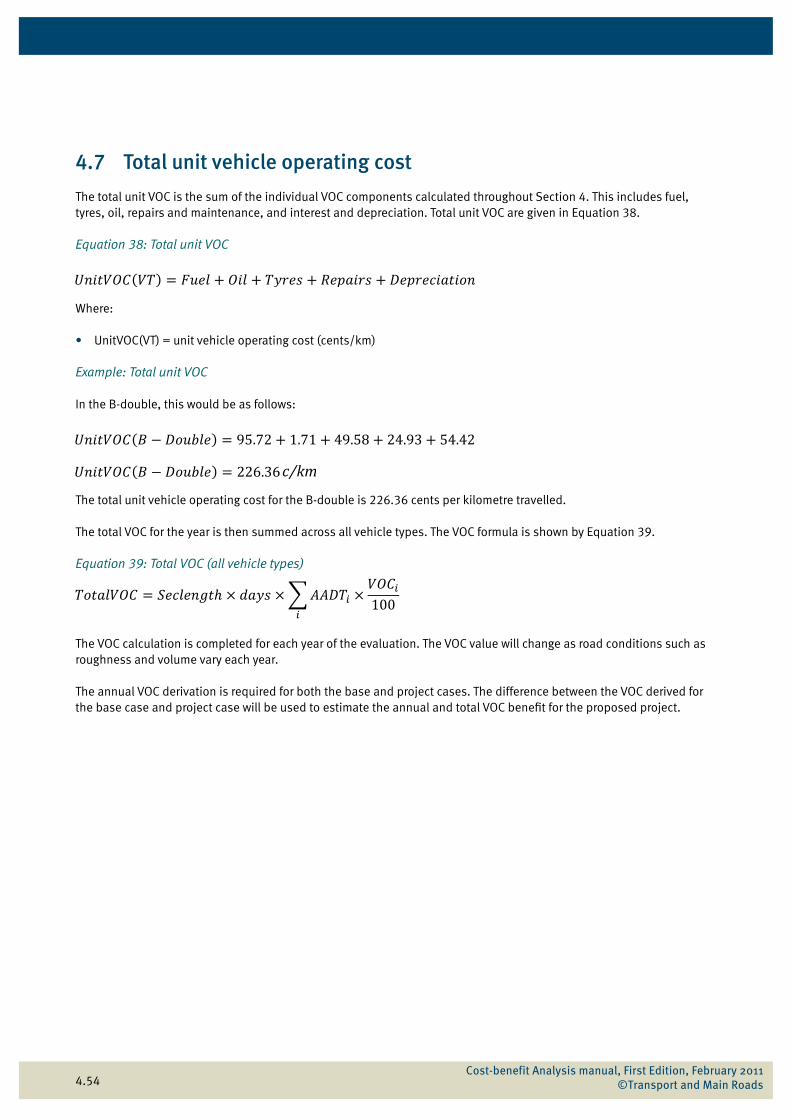
4.7 Total unit vehicle operating cost

The total unit VOC is the sum of the individual VOC components calculated throughout Section 4. This includes fuel, tyres, oil, repairs and maintenance, and interest and depreciation. Total unit VOC are given in Equation 38.

Equation 38: Total unit VOC

Where:

• UnitVOC(VT) = unit vehicle operating cost (cents/km)

Example: Total unit VOC

In the B-double, this would be as follows:

The total unit vehicle operating cost for the B-double is 226.36 cents per kilometre travelled.

The total VOC for the year is then summed across all vehicle types. The VOC formula is shown by Equation 39.

Equation 39: Total VOC (all vehicle types)

The VOC calculation is completed for each year of the evaluation. The VOC value will change as road conditions such as roughness and volume vary each year.

The annual VOC derivation is required for both the base and project cases. The difference between the VOC derived for the base case and project case will be used to estimate the annual and total VOC benefit for the proposed project.

100


Documents

4 Vehicle operating costs