3D reconstructionclass 11

Multiple View GeometryComp 290-089Marc Pollefeys

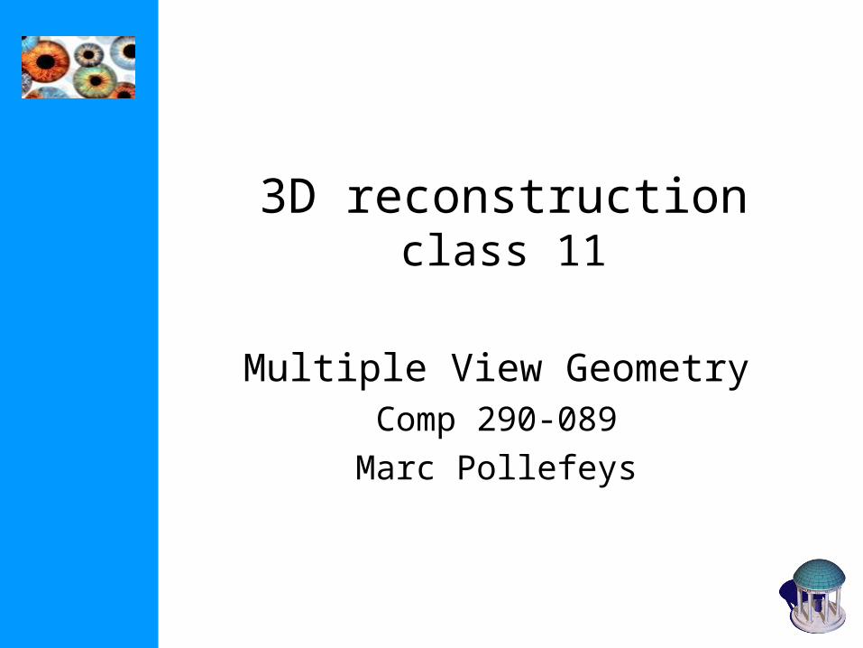
Multiple View Geometry course schedule(subject to change)

Jan. 7, 9 Intro & motivation Projective 2D Geometry

Jan. 14, 16

(no class) Projective 2D Geometry

Jan. 21, 23

Projective 3D Geometry (no class)

Jan. 28, 30

Parameter Estimation Parameter Estimation

Feb. 4, 6 Algorithm Evaluation Camera Models

Feb. 11, 13

Camera Calibration Single View Geometry

Feb. 18, 20

Epipolar Geometry 3D reconstruction

Feb. 25, 27

Fund. Matrix Comp. Structure Comp.

Mar. 4, 6 Planes & Homographies Trifocal Tensor

Mar. 18, 20

Three View Reconstruction

Multiple View Geometry

Mar. 25, 27

MultipleView Reconstruction

Bundle adjustment

Apr. 1, 3 Auto-Calibration Papers

Apr. 8, 10

Dynamic SfM Papers

Apr. 15, 17

Cheirality Papers

Apr. 22, 24

Duality Project Demos

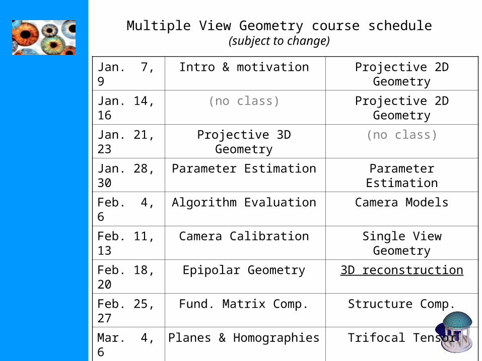
Two-view geometry

Epipolar geometry

3D reconstruction

F-matrix comp.

Structure comp.

(i) Correspondence geometry: Given an image point x in the first image, how does this constrain the position of the

corresponding point x’ in the second image?

(ii) Camera geometry (motion): Given a set of corresponding image points {xi ↔x’i}, i=1,…,n, what are the cameras P and P’ for the two views?

(iii) Scene geometry (structure): Given corresponding image points xi ↔x’i and cameras P, P’, what is the position of (their pre-image) X in space?

Three questions:

C1

C2

l2

P

l1

e1

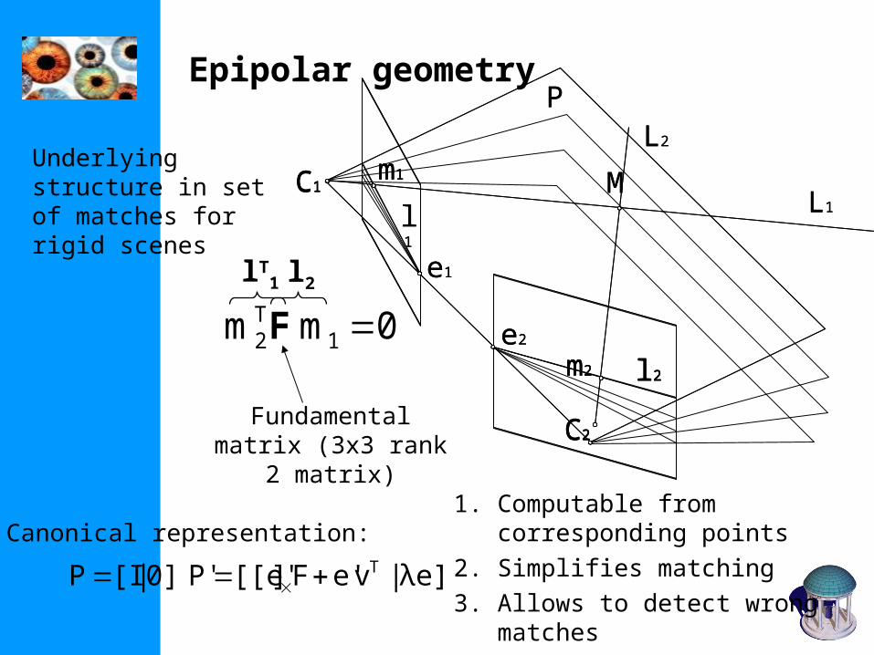
e20m m 1T2 F

Fundamental matrix (3x3 rank 2

matrix)1. Computable from

corresponding points2. Simplifies matching3. Allows to detect wrong

matches4. Related to calibration

Underlying structure in set of matches for rigid scenes

l2

C1m1

L1

m2

L2

M

C2

m1

m2

C1

C2

l2

P

l1

e1

e2

m1

L1

m2

L2

M

l2lT1

Epipolar geometry

Canonical representation:

]λe'|ve'F][[e'P' 0]|[IP T

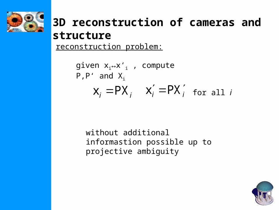
3D reconstruction of cameras and structure

given xi↔x‘i , compute P,P‘ and Xi

reconstruction problem:

ii PXx ii XPx for all i

without additional informastion possible up to projective ambiguity

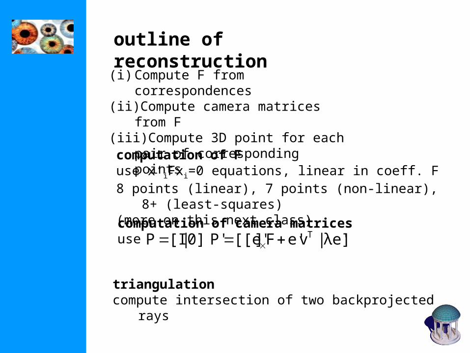
outline of reconstruction

(i) Compute F from correspondences(ii) Compute camera matrices from F(iii) Compute 3D point for each pair of

corresponding points

computation of Fuse x‘iFxi=0 equations, linear in coeff. F8 points (linear), 7 points (non-linear), 8+ (least-squares)(more on this next class)

computation of camera matricesuse ]λe'|ve'F][[e'P' 0]|[IP T

triangulationcompute intersection of two backprojected rays

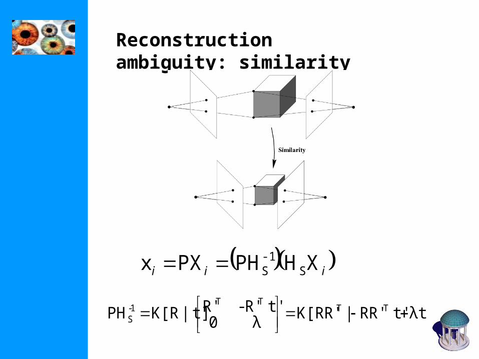
Reconstruction ambiguity: similarity

iii XHPHPXx S-1S

λt]t'RR'|K[RR'λ0

t'R'-R' t]|K[RPH TTTT

1-S

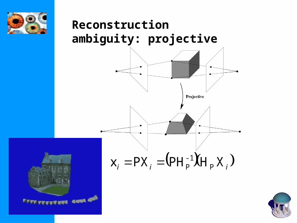
Reconstruction ambiguity: projective

iii XHPHPXx P-1

P

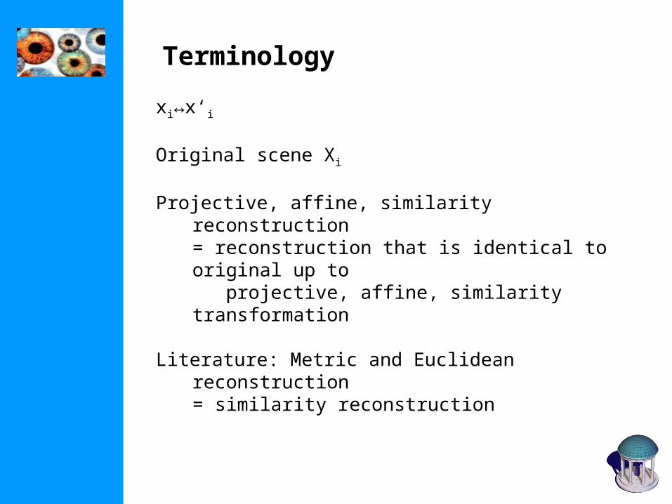
Terminology

xi↔x‘i

Original scene Xi

Projective, affine, similarity reconstruction = reconstruction that is identical to original up to projective, affine, similarity transformation

Literature: Metric and Euclidean reconstruction = similarity reconstruction

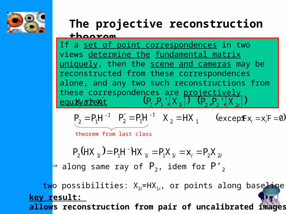
The projective reconstruction theorem

If a set of point correspondences in two views determine the fundamental matrix uniquely, then the scene and cameras may be reconstructed from these correspondences alone, and any two such reconstructions from these correspondences are projectively equivalent

i111 X,'P,P i222 X,'P,Pii xx -1

12 HPP -112 HPP

12 HXX 0FxFx :except ii

theorem from last class

iiiii 22111-1

112 XPxXPHXHPHXP along same ray of P2, idem for P‘2

two possibilities: X2i=HX1i, or points along baseline

key result: allows reconstruction from pair of uncalibrated images

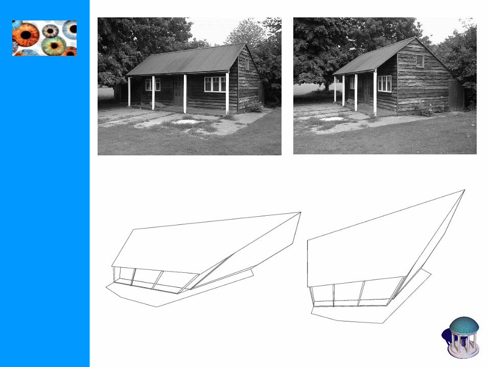
Stratified reconstruction

(i) Projective reconstruction(ii) Affine reconstruction(iii) Metric reconstruction

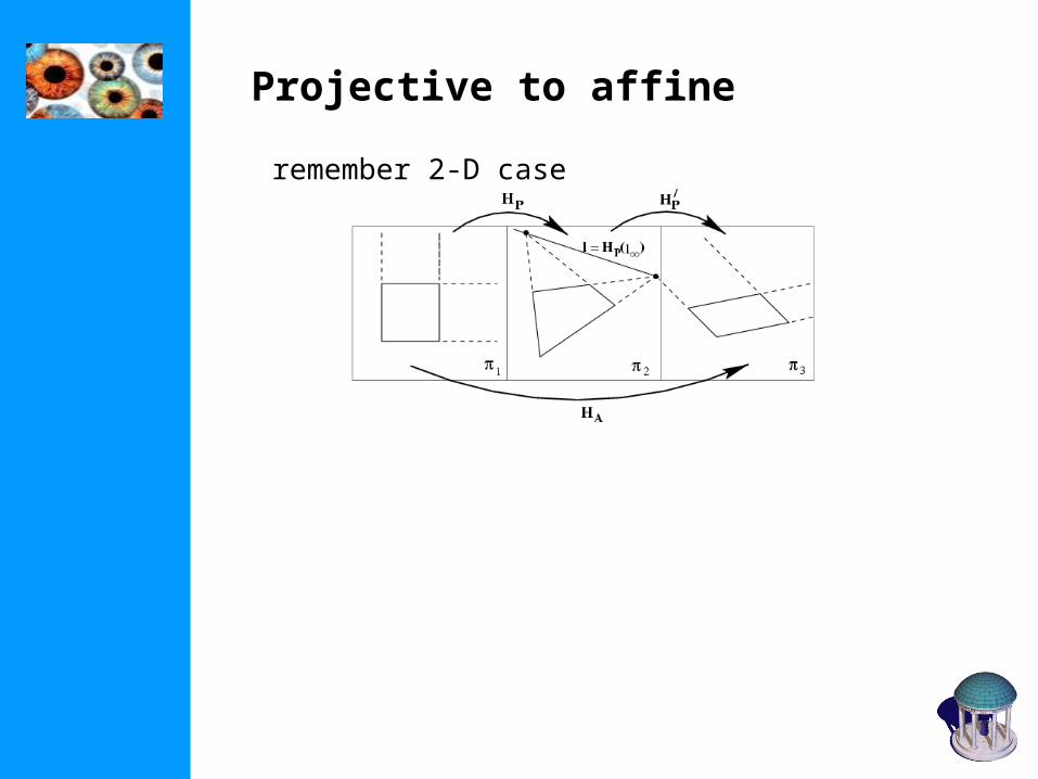
Projective to affine

remember 2-D case

Projective to affine

iX,P'P,

TT 1,0,0,0,,,π DCBA

TT 1,0,0,0πH-

π0|I

H (if D≠0)

theorem says up to projective transformation, but projective with fixed ∞ is affine transformation

can be sufficient depending on application, e.g. mid-point, centroid, parallellism

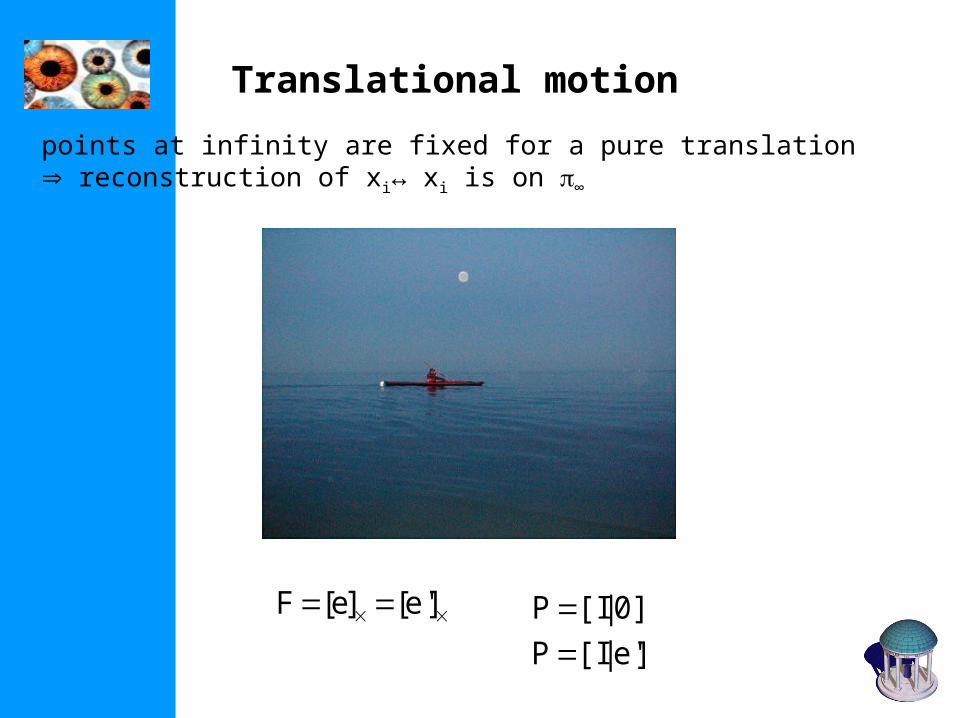
Translational motion

points at infinity are fixed for a pure translation reconstruction of xi↔ xi is on ∞

]e'[]e[F 0]|[IP ]e'|[IP

Scene constraints

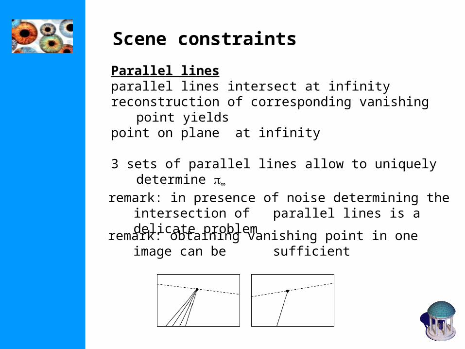
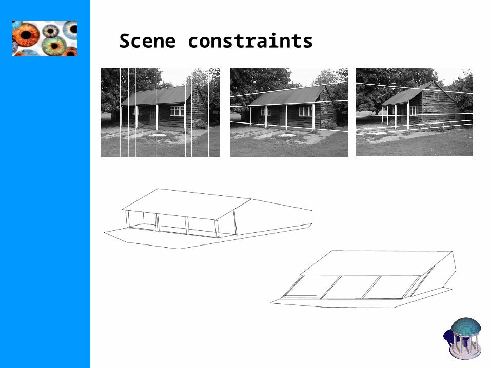
Parallel linesparallel lines intersect at infinityreconstruction of corresponding vanishing point yields point on plane at infinity

3 sets of parallel lines allow to uniquely determine ∞

remark: in presence of noise determining the intersection of parallel lines is a delicate problem

remark: obtaining vanishing point in one image can be sufficient

Scene constraints

Scene constraints

Distance ratios on a lineknown distance ratio along a line allow to determine point at infinity (same as 2D case)

The infinity homography

∞

∞

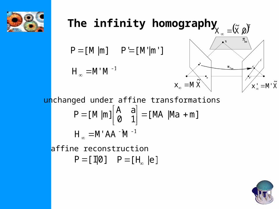
m]|[MP ]m'|[M'P'

-1MM'H

T0,X~

X

X~

Mx X~

M'x'

m]Ma|[MA10aAm]|[MP

-1-1MAAM'H

unchanged under affine transformations

0]|[IP e]|[HP affine reconstruction

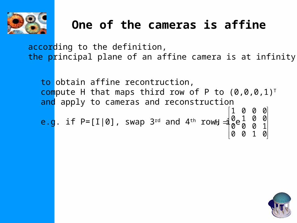
One of the cameras is affine

according to the definition, the principal plane of an affine camera is at infinity

to obtain affine recontruction, compute H that maps third row of P to (0,0,0,1)T

and apply to cameras and reconstruction

e.g. if P=[I|0], swap 3rd and 4th row, i.e.

0100100000100001

H

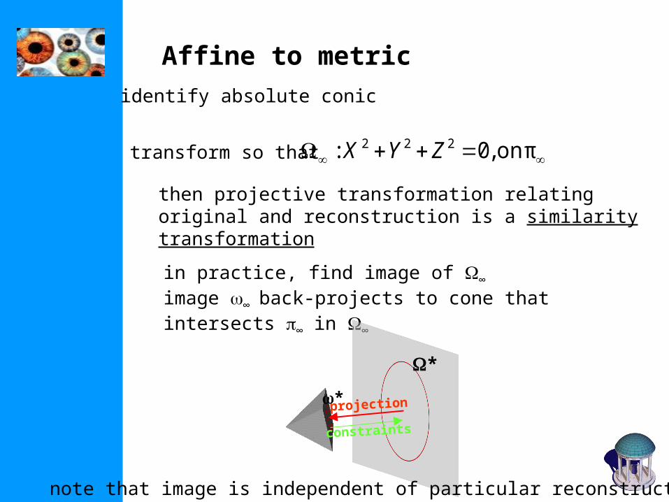
Affine to metric

identify absolute conic

transform so that on π ,0: 222 ZYX

then projective transformation relating original and reconstruction is a similarity transformation

in practice, find image of ∞ image ∞back-projects to cone that intersects ∞ in ∞

*

*

projection

constraints

note that image is independent of particular reconstruction

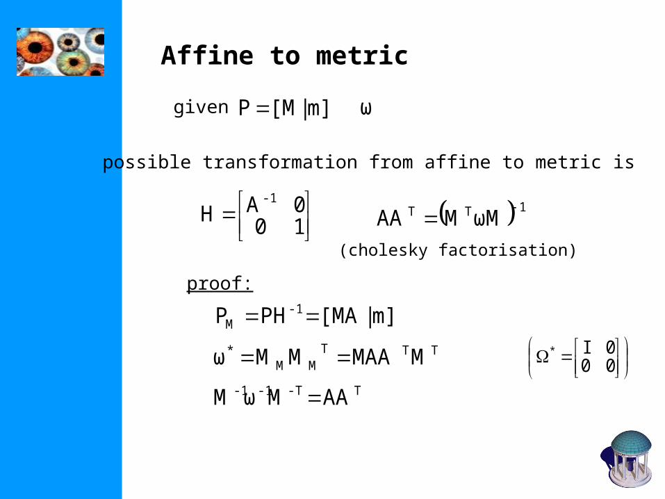
Affine to metric

m]|[MP ω

100AH

-1

given

possible transformation from affine to metric is

1TT ωMMAA

(cholesky factorisation)

m]|[MAPHP -1M

proof:

TTTMM

* MMAAMMω T-T-1-1 AAMωM

00

0I*

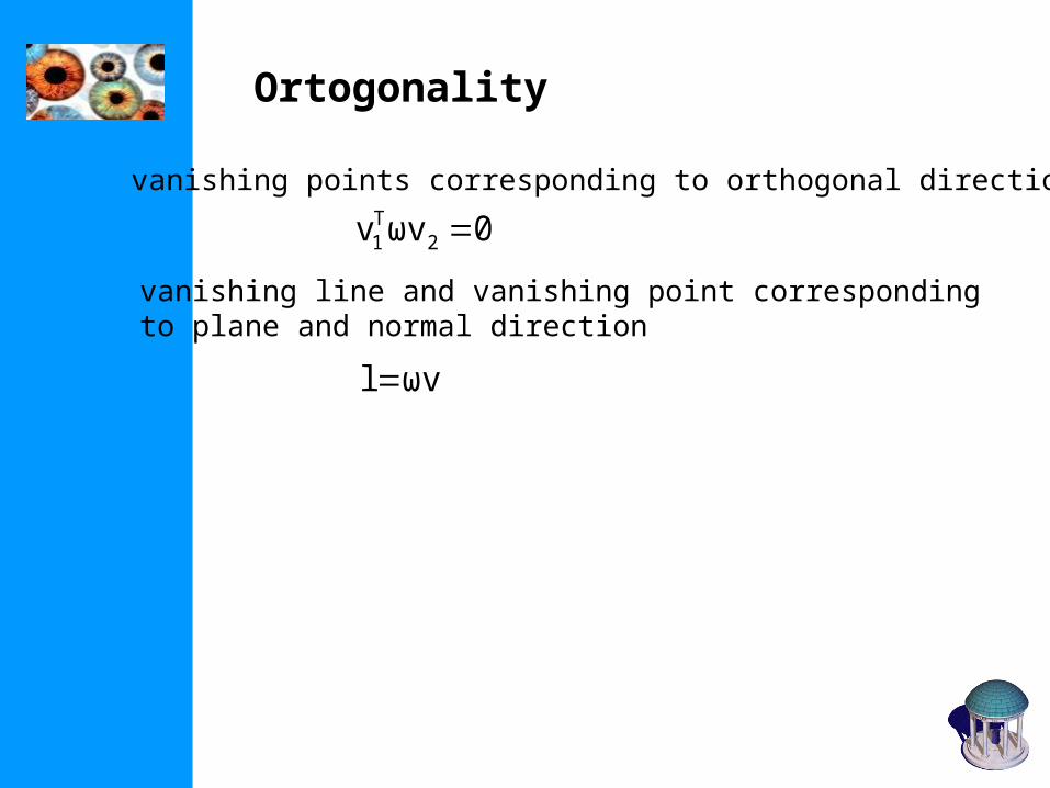
Ortogonality

0ωvv 2T1

ωvl

vanishing points corresponding to orthogonal directions

vanishing line and vanishing point corresponding to plane and normal direction

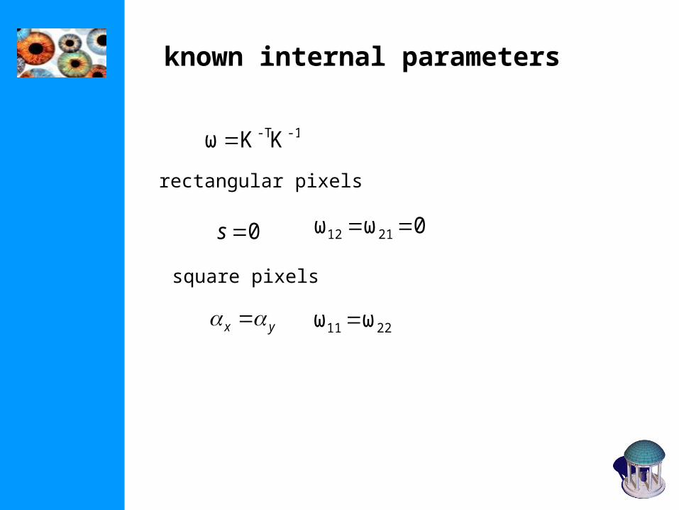
known internal parameters

-1-TKKω

0ωω 2112 0s

rectangular pixels

yx

square pixels

2211 ωω

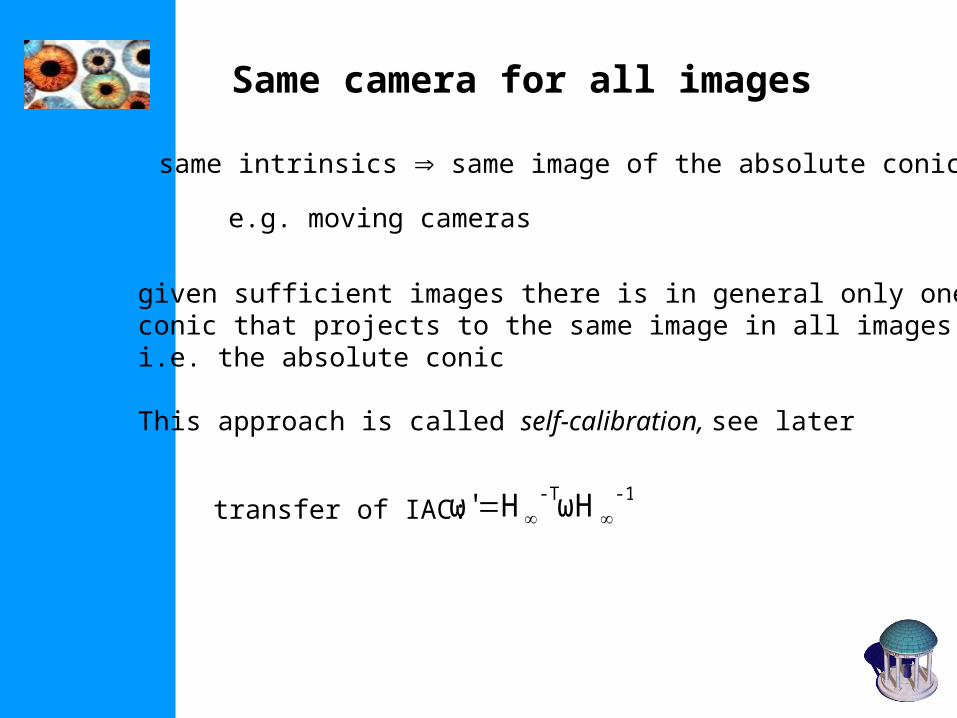
Same camera for all images

same intrinsics same image of the absolute conic

e.g. moving cameras

given sufficient images there is in general only oneconic that projects to the same image in all images,i.e. the absolute conic

This approach is called self-calibration, see later

-1-TωHHω' transfer of IAC:

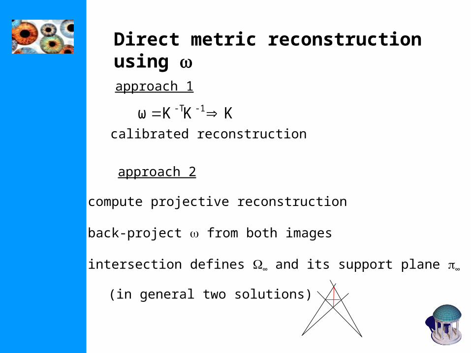
Direct metric reconstruction using

KKKω -1-T

approach 1

calibrated reconstruction

approach 2

compute projective reconstruction

back-project from both images

intersection defines ∞ and its support plane ∞

(in general two solutions)

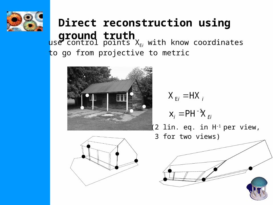
Direct reconstruction using ground truth

ii HXXE

use control points XEi with know coordinatesto go from projective to metric

Eii XPHx -1(2 lin. eq. in H-1

per view, 3 for two views)

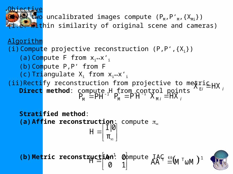
ObjectiveGiven two uncalibrated images compute (PM,P‘M,{XMi})(i.e. within similarity of original scene and cameras)

Algorithm(i) Compute projective reconstruction (P,P‘,{Xi})

(a) Compute F from xi↔x‘i(b) Compute P,P‘ from F(c) Triangulate Xi from xi↔x‘i

(ii) Rectify reconstruction from projective to metricDirect method: compute H from control points

Stratified method:(a) Affine reconstruction: compute ∞

(b) Metric reconstruction: compute IAC

ii HXXE -1

M PHP -1M HPP ii HXXM

π0|I

H

100AH

-1

1TT ωMMAA

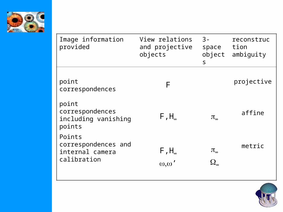
Image information provided

View relations and projective objects

3-space objects

reconstruction ambiguity

point correspondences F projective

point correspondences including vanishing points F,H∞ ∞

affine

Points correspondences and internal camera calibration

F,H∞

’

∞

∞

metric

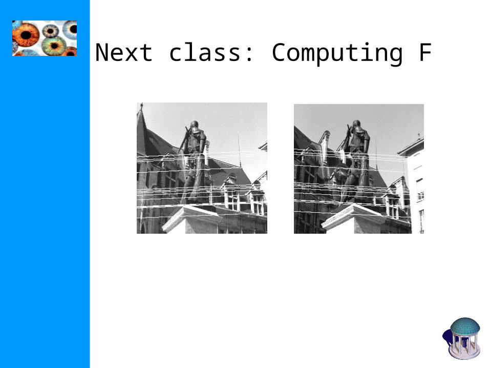
Next class: Computing F