Embed Size (px)
Citation preview
ELSJZVIER
Computer methods in applied
mechanics and engineering
Comput. Methods Appl. Mech. Engrg. 157 (1998) 115-131
3D Delaunay mesh generation coupled with an advancing-front approach
Pascal J. Frey *, Houman Borouchaki, Paul-Louis George INRIA, Domain de Voluceau, Rocquencourt, BP 105, 78153 Le Chesnay Cedex, France
Received 28 May 1996
Abstract
This paper describes a fully automatic mesh generation method suitable for domains of any shape in [w’. Initially, a so-called boundary
mesh is generated wherein internal points are created using advancing-front point placement and inserted using a Delaunay method. The
algorithm combines the advantages of efficiency and nice mathematical properties of a Delaunay approach with advancing-front high-quality
point-placement strategy. Several three-dimensional examples are presented to demonstrate the overall efficiency and the relevance of the
combined procedure. The present method can be extended to isotropic or anisotropic adaptive mesh generation. 0 1998 Elsevier Science
S.A.
1. Introduction
The generation of three-dimensional unstructured meshes has known extensive and increasing interest over the last decade. To some extent, regarding the level of maturity it has reached, it has been stated recently that
unstructured mesh generation can be considered a solved problem [l]. The statement is certainly premature, and
further developments in adaptive anisotropic meshing procedures are surely needed. Given a polyhedral discretization of its boundary, input as a list of triangular faces, several methods are likely
to provide a mesh of a domain. Unstructured mesh generation procedures commonly in use are typically based
on either a Delaunay or an advancing-front approach, both being usually described as rivals. On the contrary, this paper is an attempt to demonstrate their complementary nature, by combining their respective assets. The
Delaunay approach offers attractive mathematical properties, in particular in terms of the connectivity associated with mesh vertices. On the other hand, an advancing-front approach offers the advantages of high-quality
point-placement strategy. Such methods have been described first by Rebay [2] and Miiller et al. [3], and later taken up by Marcum et
al. [4] and Merriam et al. [5]. A general scheme and a thorough discussion of both approaches is exposed by Mavriplis [l]. These methods based on advancing-front point-placement and Delaunay connectivity have been
extensively described in two dimensions and their authors indicate they extend readily to three dimensions.
The proposed method first proceeds with a so-called boundary mesh (a constrained Delaunay empty mesh) which includes all the boundary points (similar to a Delaunay approach). Internal points are then iteratively created using an advancing-front approach and inserted using a Delaunay kernel into the existing triangulation. The overall procedure is applied repetitively until the mesh satisfies a desired element-size distribution function. The front identification is one of the main features of the proposed method and its faces must be properly
* Corresponding author
0045-7825/98/$19.00 0 1998 Elsevier Science S.A. All rights reserved
PII SOO45-7825(97)00222-3
116 P.J. Frey et al. I Comput. Methods Appl. Mech. Engrg. 157 (1998) 115-131
characterized to ensure the optimal convergence of the algorithm. The final mesh quality is then improved using standard optimization techniques [6]. The resulting mesh will be used in numerical finite element simulations which will eventually decide of mesh adaptation. This approach can be extended to the anisotropic mesh
generation case, where the element sizes are computed in a non-Euclidean (i.e. Riemannian) metric in such a way as to take into account both directional and size specifications [‘7].
In the following sections, the different steps toward mesh generation are presented along with numerical
results and statistics. Section 2 describes the general scheme of the mesh generation algorithm. The Delaunay kernel is introduced in Section 3. Within Section 4 the principle of the boundary mesh generation is briefly
described. The identification of the front and a complete description of the field point generation and insertion are discussed in Section 5, while optimization techniques are recalled in Section 6. Main lines of an adaptive
mesh generation scheme are given in Section 7. Application examples are discussed in Section 8. To conclude,
in Section 9 future trends and open problems are indicated.
2. Scheme of the method
Usually, Delaunay or advancing-front mesh generation methods start from the sole data of a discretization of the domain boundaries as a set of edges and faces in three dimensions. Thus, the mesh of the domain is only
governed by geometric considerations, whatever the physic of the problem under consideration. Sizes as well as element densities are related to the given boundary discretization.
Let us consider a domain of any shape in Iw3 and 9 the set of constrained edges and faces defining the boundary of this domain. These items have as endpoints a set of points, denoted as 9
To mesh the domain, a buwdury mesh is generated at first, which is, following [8], a mesh whose sole
vertices are the members of Y. A new mesh is obtained by adding field points inside the previous mesh and then optimized so as to complete the final mesh of the domain. The field points are defined and inserted iteratively
into the existing triangulation, the initial mesh being the boundary mesh. In the described method, similar to the conventional advancing-front method, the front is identified and internal points are created to form optimal
tetrahedral elements in accordance with an element-size distribution function. A Delaunuy kernel procedure is
used to insert these points into the existing triangulation. The corresponding scheme of the mesh generation algorithm can be described as follows:
Mesh generation scheme
(1) Creation of the boundary mesh T( 9, 9). l creation of B a box enclosing the domain;
l mesh r( 3) of the bounding box 5%; l insertion of the points of Y into T( 3) to define mesh T( 3, 9); l regeneration of 9, the constrained edges and faces, in T( B, Y) to define mesh T( B, Y, 9); l identification of boundary mesh T( 9, 9) in T( %‘, 9, 9).
(2) Creation of mesh T.
l initialization of mesh T with T(Y, 9);
l initialization of front with faces of P, l Field point creation (loop)
- generation of points from the front face; - insertion of these points into T, - identification of the new front; - process repeated until front is empty.
(3) Optimization of T. Each of these steps is briefly described in the following sections. First is detailed how to construct the
boundary mesh using an incremental point insertion process, the so-called Delaunuy kernel. The use of the Delaunay kernel to construct a mesh whose vertices are the point of Y is shown as well as the way in which the constrained items of 9 can be generated to produce the boundary mesh. Afterwards, the field point creation and insertion are described step-by-step.
P.J. Frey et al. I Comput. Methods Appl. Mech. Engrg. 157 (1998) 115-131 117
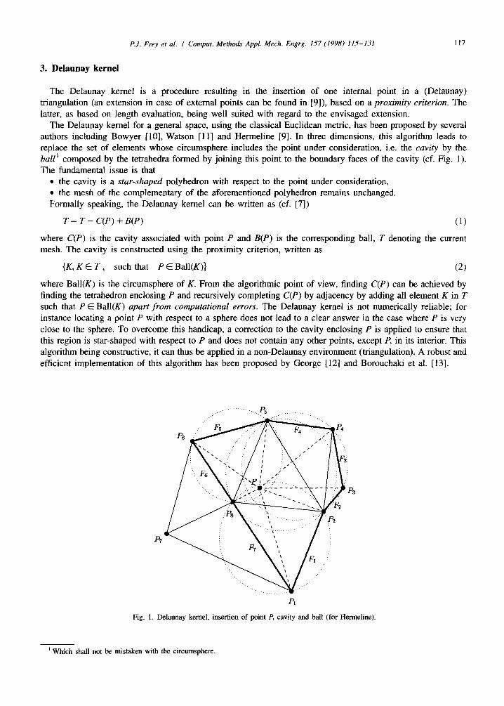
3. Delaunay kernel
The Delaunay kernel is a procedure resulting in the insertion of one internal point in a (Delaunay)
triangulation (an extension in case of external points can be found in [9]), based on a proximity criterion. The latter, as based on length evaluation, being well suited with regard to the envisaged extension.
The Delaunay kernel for a general space, using the classical Euclidean metric, has been proposed by several authors including Bowyer [lo], Watson [l l] and Hermeline [9]. In three dimensions, this algorithm leads to replace the set of elements whose circumsphere includes the point under consideration, i.e. the cavity by the ball’ composed by the tetrahedra formed by joining this point to the boundary faces of the cavity (cf. Fig. 1). The fundamental issue is that
l the cavity is a star-shaped polyhedron with respect to the point under consideration,
l the mesh of the complementary of the aforementioned polyhedron remains unchanged. Formally speaking, the Delaunay kernel can be written as (cf. [7])
T=T-C(P)+B(P) (1)
where C(P) is the cavity associated with point P and B(P) is the corresponding ball, T denoting the current mesh. The cavity is constructed using the proximity criterion, written as
{K, K E T , such that P E Ball(K)} (2)
where Ball(K) is the circumsphere of K. From the algorithmic point of view, finding C(P) can be achieved by
finding the tetrahedron enclosing P and recursively completing C(P) by adjacency by adding all element K in T
such that P E Ball(K) apart from computational errors. The Delaunay kernel is not numerically reliable; for instance locating a point P with respect to a sphere does not lead to a clear answer in the case where P is very
close to the sphere. To overcome this handicap, a correction to the cavity enclosing P is applied to ensure that this region is star-shaped with respect to P and does not contain any other points, except P, in its interior. This algorithm being constructive, it can thus be applied in a non-Delaunay environment (triangulation). A robust and
efficient implementation of this algorithm has been proposed by George [12] and Borouchaki et al. [13].
. . . 4
Pl
Fig. 1. Delaunay kernel, insertion of point P, cavity and ball (for Hermeline).
’ Which shall not be mistaken with the circumsphere.
118 P.J. Frey et al. I Comput. Methods Appl. Mech. Engrg. 157 (1998) 115-131
4. Boundary mesh generation
The boundary mesh generation includes three successive steps described below.
4.1. Bounding box mesh
Introducing a bounding box encompassing the domain allows us to be in a convex environment such that all the boundary points are enclosed within it. The box is defined using eight vertices and covered with a mesh
T( %‘) consisting of five tetrahedra. The points of Y are inserted into T( 3,) using the Delaunay kernel, resulting
in the mesh T( 3, 9”). Usually, except under specific conditions concerning the regularity of the domain, the whole set of constrained items of 9 being not present in this mesh, a procedure based on local mesh modifications is used to regenerate the missing items in T( $8, 9”).
4.2. Boundary conforming mesh
The bounding box mesh generally does not contain in the edge and face lists of its elements all the entities constituting the given boundary. Subsequently, we cannot properly define the domain, the notions of interior and
exterior can only be specified with respect to the given boundary. The regeneration of the boundary in the box mesh is a complex problem which can be defined in many ways and several solutions can be proposed. Currently, there is no formal proof of the existence of a solution (the Schijnart polyhedron is an example of
polyhedron which cannot be triangulated without adding internal point. This simple example gives a rough idea of the difficult task of recovering the boundary). Nevertheless, we propose a method to regenerate the boundary and refer to [9,14] in which different approaches are investigated.
The basic idea is to locally transform the mesh in order to regenerate the missing entities in 9, using a
property of equivalence among the different possible triangulations of a polyhedron. It is a question of defining
topological and geometrical operators allowing to delete an edge or a face intersected by a missing entity, and in few cases to create internal points (Steiner points). The latter being then considered as Source points (e.g.
user-specified points).
4.3. Boundary mesh identijcation
Once all constrained entities of 9 have been integrated in T( 9, Y’), T( 9, 9, S) is obtained. The mesh
r( 9, S) of the domain is identified by means of its complement in T( 3, Y, 9). Boundary mesh creation implies to have control of the notions of interior and exterior with respect to the domain. Starting from a
tetrahedron having one of the eight extra vertices as vertex, the complement of T(Y, S) in T( 3, 9, 9”) is
identified by adjacency.
REMARK. A boundary mesh can be obtained through any meshing procedure (see, for instance, Marcum et al. [4]). Afterwards, we assume the so-called boundary mesh is obtained using the proposed procedure.
5. Advancing-front method
At first, we describe the standard advancing-front method. Derived from this technique, the field point
generation strategy is then detailed in the following sections.
5.1. ‘Classical’ approach
Suitable for arbitrary geometries, a mesh generator of the present class constructs the covering-up of a domain by tetrahedral elements, from its boundary discretization. In practice, a polyhedral approximation of the boundary is used which consists of a list of triangular faces mixed, if need be, with user-specified vertices, edges and faces considered as constrained entities to be respected by the mesh. The method involves the simultaneous
P.J. Frey et al. I Comput. Methods Appl. Mech. Engrg. 157 (1998) 115-131 119
generation of mesh points and their connectivity. It usually relies on an explicitly defined element-size function
(size map), which is most often obtained using a background grid [ 15-171.
The process is iterative; a front, initialized by the set of faces of the given boundary, is analyzed in order to
determine a departure face from which one or several elements are created. The front is then updated and the process repeated until the front is empty (i.e. when all fronts have merged upon each other and the domain is entirely covered). The process can be summarized as follows
General scheme
l initialization of the front,
l creation of internal element (loop) - determination of the departure face (based on various criteria, for instance the smallest face); - analysis of this entity and creation of internal point(s); - creation of new connections; _ update the front;
l repeat the creation loop as long as the front is not empty.
The analysis of the front and the way in which the internal points are created can be performed in several
ways. As can be seen, the efficiency and the reliability of the method is strongly related to the way the space is known. It is critical to find the context relative to a face of the front quickly, i.e. to know the neighborhood of any front face and that of any tetrahedron of the mesh in progress. One of the solutions is to create a grid enclosing the domain, the cells of this grid referencing the useful information. This neighborhood space is
usually chosen as a regular grid or an ‘octree’. To govern the internal point creation and connected element
creation phase, a control space is introduced. Thus, a face of the front is considered, via the neighborhood space, its environment is known and, via the control space, the nature of the element to be created is determined
(for instance the desired shape).
In brief, the critical features of such methods are related to the issues of knowing where we are and what we
are supposed to do at a given step. This brings up the problem of spatial locating and optimal tetrahedron
construction from a given front face. In addition, the point creation process requires the determination whether
the point falls or not into the domain and if so, whether it intersects any existing element. On the contrary, an heuristic method must replace this point by a valid one from the front. If the method fails to find such a point,
the current front is then modified and the process repeated. The main difficulty is the lack of background information in point placement. In three dimensions, the implementation of an efficient and robust advancing-
front method suitable for the creation of elements satisfying the desirable criteria is a complex task which requires great care. This is the reason why only a few 3D mesh generators of this class are really efficient [S].
In an attempt to overcome this difficult task, we suggest to use the Delaunay boundary mesh as a background grid and the Delaunay kernel as an insertion tool that make the insertion of the field points created using an advancing-front point-placement strategy possible. Thus the convergence of the process is always ensured, the
remaining critical feature being the identification of the front (while in the classical approach, the front is
automatically identified).
5.2. Front identijcation
As mentioned in the previous section, the problem we must face is to identify and update the front. With the conventional advancing-front method, the explicit management of front faces is required. Thus, either an element is formed with the selected faces, or an internal point is created which allows the creation of the elements by simply joining it to the selected faces. A new state of front is formed by
l removing the faces of front belonging to a tetrahedron created from the present front; l adding the faces of the newly created tetrahedra, in the case where these faces are not common to two
elements.
The front is automatically defined through this procedure.
In our approach, the triangulation at state i is constructed (see general scheme, internal point creation loop, Section 2), and the front is identified in order to build the triangulation at stage i + 1. The front F, at stage i
simply takes the form of a set of boundary faces between two elements, one is said to be acceptable (nicely
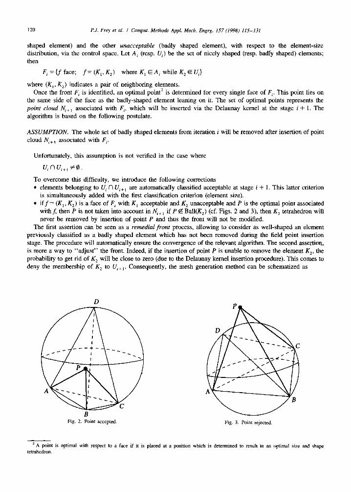
120 P.J. Frey et al. I Comput. Methods Appl. Mech. Engrg. 157 (1998) 115-131
shaped element) and the other unacceptable (badly shaped element), with respect to the element-size distribution, via the control space. Let Ai (resp. U,) be the set of nicely shaped (resp. badly shaped) elements; then
F,=Cfface; f=(Kr,K*) whereK,EAiwhileK,EUi}
where (K,, K,) indicates a pair of neighboring elements. Once the front E’, is identified, an optimal point* is determined for every single face of Fi. This point lies on
the same side of the face as the badly-shaped element leaning on it. The set of optimal points represents the point cloud Ni+ I associated with Fi, which will be inserted via the Delaunay kernel at the stage i + 1. The algorithm is based on the following postulate.
ASSUMPTION. The whole set of badly shaped elements from iteration i will be removed after insertion of point cloud N,,, associated with F,.
Unfortunately, this assumption is not verified in the case where
To overcome this difficulty, we introduce the following corrections l elements belonging to U, II Ui + 1 are automatically classified acceptable at stage i + 1. This latter criterion
is simultaneously added with the first classification criterion (element size). l if f = (K, , K,) is a face of Fi with K, acceptable and K, unacceptable and P is the optimal point associated
with 5 then P is not taken into account in Ni + 1 if P 62 Ball(K,) (cf. Figs. 2 and 3), then K, tetrahedron will never be removed by insertion of point P and thus the front will not be modified.
The first assertion can be seen as a remedial front process, allowing to consider as well-shaped an element previously classified as a badly shaped element which has not been removed during the field point insertion stage. The procedure will automatically ensure the convergence of the relevant algorithm. The second assertion, is more a way to “adjust” the front. Indeed, if the insertion of point P is unable to remove the element K2, the probability to get rid of K2 will be close to zero (due to the Delaunay kernel insertion procedure). This comes to deny the membership of K2 to Vi+ 1. Consequently, the mesh generation method can be schematized as
B Fig. 2. Point accepted. Fig. 3. Point rejected.
’ A point is optimal with respect to a face if it is placed at a position which is determined to result in an optimal size and shape tetrahedron.
P.J. Frey et al. I Comput. Methods Appl. Mech. Engrg. 157 (1998) 115-131 121
Scheme of the mesh generator
l initializations
-F,=$,i= I;
l while Fi_, Z0
- loop over faces f of Fi_ I ;
f=(K,,Kz), K, EA;_I, ‘2E’i-l * compute location of P, optimal point associated with f; * store P in N; if P E Ball(K,);
l filtration of N,; l creation of T, by inserting N, in Ti_ , ; l identification of F,;
-loop over K, K 12 Ai_1
* if KElJ_, then KEA,_,; * else K classified according to a classification criterion (see section below);
l increment i.
REMARKS. The initial front contains the boundary faces of the domain. This is equivalent to classifying all
external (resp. internal) tetrahedra as well-shaped (resp. bad-shaped) elements, defining thus the set A,, (resp. U,). During the insertion of Ni in Ti _ 1, members of A i _ 1 can be removed. In this scheme, we still have to define
the classification criterion and the filtration of field points process.
Classijkation criterion. An element is said to be acceptable if its edge lengths are optimal with respect to the
given size map (this seems to be the most reasonable way to classify the elements). Notice that with any other exclusive criterion (for instance based on the circumsphere radius, cf. Rebay [2]), the aforementioned
assumption is generally not verified. Let K be a tetrahedron. K is classified as acceptable if and only if
Va edge of K l(a)<&
where l(a) is the normalized edge length of a with respect to the control space.
Filtration of the field points. As every point of Ni point cloud is created apart from the others, a filtration process can remove from Ni a point which violates the size criterion (via the control space) when compared with
a previously selected point of Ni. Let Q be an arbitrary point of &, different from I? Q is filtered if and only if there exists a selected point P of
Ni such that
5.3. Optimal point-creation and point-placement
As mentioned in the scheme (see previous section), we describe now the optimal point creation with respect to
a front face, leading to the creation of an ideal tetrahedron. This latter being identified through the control space.
Thus, we l describe the control space; l introduce the notion of normalized length; and l define the ideal tetrahedron (via this space) based on a front face and propose a method to construct this
element.
5.3.1. Control space
The control space associated with a given domain 64 of Iw3 is by definition 0 supplied with a continuous size field. This space can be defined from a mesh of fl and a discrete size field associated with every single vertex of this mesh, namely a background mesh. Using an interpolation of the discrete field with respect to the mesh, it is then possible to derive a continuous size field.
122 P.J. Frey et al. 1 Comput. Methods Appl. Mech. Engrg. 157 (1998) 115-131
The background mesh is defined by the boundary mesh T( 9, 9) of the domain. To obtain the discrete field associated with the mesh vertices, it is only needed to define the size at every vertex. Let P be a vertex of the
background mesh, l if P is a vertex of F, then the size at P can be defined by
h(P) = I,,,(‘) + ‘ma,tp)
2
where Zmi,(P) (resp. Z,,,(P)) represents the euclidian edge length of the largest (resp. smallest) edge of F
connected to P,
l if P is a Steiner point, then
where a represents the set of edges having P as endpoint and h, is the requested size at the vertex opposite to P along the edge a.
Subsequently, the discrete size map is well defined. For every point Q of 0, a tetrahedron K exists in the background mesh enclosing it. Let (c~~i)(r~~~~) be the barycentric coordinates of Q in K, then h(Q) can be defined by the way of an arithmetic interpolation
4
h(Q) = C aih(Pi) i=l
where Pi, (1 C i < 4) are the vertices of K.
REMARK. In this case the background mesh is an invariant defined by the boundary mesh of the domain T( 9, 9). An alternate solution is to consider the T _ , as the background mesh for the insertion of the points of
Ni. This is equivalent to modifying the size field at each iteration of the generation of a point cloud associated with a front.
The normalized edge length of any edge of the current mesh can be estimated through this control space.
5.3.2. Normalized edge length computation
Let AB be a mesh edge. To compute the normalized edge length of AB, it is required to know the size specification along this edge. To this end, the edge is embedded in the background mesh and every intersection
point with a tetrahedron face represents a size specification along the edge. In a similar manner, the size specification at both ends of AB is determined through the background mesh. Let us assume that the intersection
with the tetrahedra of the background mesh is an empty set. The only information along AB is given by h(A) and h(B). Under this assumption, the normalized edge length Z(AB) of AB is defined by
I(AB) = d(AB) O’ j& dt i
where d(AB) is the Euclidean length of AB and
h(t) = h(A) + [h(B) - h(A)]t .
We obtain finally
d(AB ) ‘CAB) = h(B) _ h(A) log
In case of a very tiny variation between h(A) and h(B), (such as for instance, 0.9 < h,/h, < l.l), it is possible to simplify the previous formula and thus write
d(AB) E(AB) = 2 h(A) + h(B) ’
P.J. Frey et al. I Comput. Methods Appt. Mech. Engrg. 157 (1998) 115-131 123
Let us assume now that AB intersects the faces of the tetrahedral elements of the background mesh in m
points (Ci),<,+. Let us consider C, = A and C,,, + 1 = B, therefore we have
m
L(AB) = 2 l(C,C,+,) ; r=O
the size at any intersection point C, is well defined and the quantities l(C,C,+ , ) can be estimated through the previous formula.
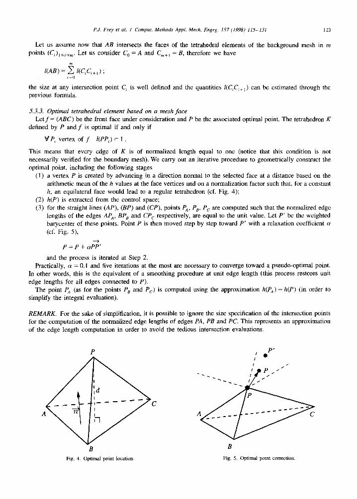
5.3.3. Optimal tetrahedral element based on a mesh face
Let f = (ABC) be the front face under consideration and P be the associated optimal point. The tetrahedron K
defined by P and f is optimal if and only if
V Pi vertex of f Z(PPi) = 1 .
This means that every edge of K is of normalized length equal to one (notice that this condition is not necessarily verified for the boundary mesh). We carry out an iterative procedure to geometrically construct the
optimal point, including the following stages
(1)
(2) (3)
a vertex P is created by advancing in a direction normal to the selected face at a distance based on the
arithmetic mean of the h values at the face vertices and on a normalization factor such that, for a constant h, an equilateral face would lead to a regular tetrahedron (cf. Fig. 4);
h(P) is extracted from the control space;
for the straight lines (AP), (BP) and (CP), points PA, PB, Pc are computed such that the normalized edge lengths of the edges AP,, BP, and CPc respectively, are equal to the unit value. Let P’ be the weighted barycenter of these points. Point P is then moved step by step toward P’ with a relaxation coefficient LY
(cf. Fig. 5),
and the process is iterated at Step 2.
Practically, (Y = 0.1 and five iterations at the most are necessary to converge toward a pseudo-optimal point. In other words, this is the equivalent of a smoothing procedure at unit edge length (this process restores unit
edge lengths for all edges connected to P).
The point P, (as for the points P, and Pc) is computed using the approximation h(P,) = h(P) (in order to simplify the integral evaluation).
REMARK. For the sake of simplification, it is possible to ignore the size specification of the intersection points
for the computation of the normalized edge lengths of edges PA, PB and PC. This represents an approximation
of the edge length computation in order to avoid the tedious intersection evaluations.
Fig. 4. Optimal point location. Fig. 5. Optimal point correction
124 P.J. Frey et al. I Comput. Methods Appl. Mech. Engrg. 157 (1998) 115-131
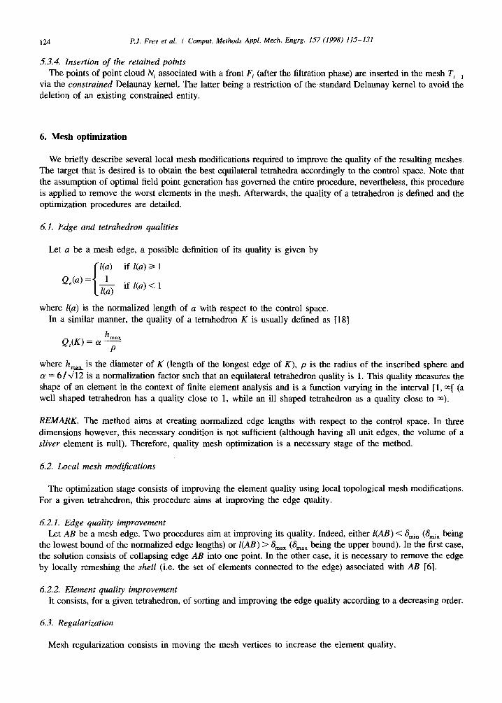
5.3.4. Insertion of the retained points
The points of point cloud Ni associated with a front F, (after the filtration phase) are inserted in the mesh Ti_I
via the constrained Delaunay kernel. The latter being a restriction of the standard Delaunay kernel to avoid the
deletion of an existing constrained entity.
6. Mesh optimization
We briefly describe several local mesh modifications required to improve the quality of the resulting meshes. The target that is desired is to obtain the best equilateral tetrahedra accordingly to the control space. Note that
the assumption of optimal field point generation has governed the entire procedure, nevertheless, this procedure
is applied to remove the worst elements in the mesh. Afterwards, the quality of a tetrahedron is defined and the optimization procedures are detailed.
6.1. Edge and tetrahedron qualities
Let a be a mesh edge, a possible
if l(a) 2 1
if Z(a) < 1
definition of its quality is given by
where l(a) is the normalized length of a with respect to the control space.
In a similar manner, the quality of a tetrahedron K is usually defined as [ 181
Q,(K) = (Y +
where h,,, is the diameter of K (length of the longest edge of K), p is the radius of the inscribed sphere and
LY = 6/a is a normalization factor such that an equilateral tetrahedron quality is 1. This quality measures the shape of an element in the context of finite element analysis and is a function varying in the interval [l, m[ (a
well shaped tetrahedron has a quality close to 1, while an ill shaped tetrahedron as a quality close to m).
REMARK. The method aims at creating normalized edge lengths with respect to the control space. In three
dimensions however, this necessary condition is not sufficient (although having all unit edges, the volume of a sEiver element is null). Therefore, quality mesh optimization is a necessary stage of the method.
6.2. Local mesh modijcations
The optimization stage consists of improving the element quality using local topological mesh modifications. For a given tetrahedron, this procedure aims at improving the edge quality.
62.1. Edge quality improvement
Let AB be a mesh edge. Two procedures aim at improving its quality. Indeed, either Z(AB) < Smin (&, being the lowest bound of the normalized edge lengths) or Z(AB) > a,,,,, (a,,, being the upper bound). In the first case,
the solution consists of collapsing edge AB into one point. In the other case, it is necessary to remove the edge by locally remeshing the shell (i.e. the set of elements connected to the edge) associated with AB [6].
6.2.2. Element quality improvement
It consists, for a given tetrahedron, of sorting and improving the edge quality according to a decreasing order.
6.3. Regularization
Mesh regularization consists in moving the mesh vertices to increase the element quality.
P.J. Frey er al. f Comput. Methods Appl. Mech. Engrg. 157 (1998) 115-131 125
Let P be a free vertex3 and B(P) be the ball associated with P. (i.e. the set of elements sharing P). This latter
constitutes a star-shaped polyhedron with respect to P. We relocate P to increase the quality of B(P) (in
particular that of its worst element). Two methods are usually envisaged, Laplacian smoothing and optimal
smoothing. Afterwards only this latter is described.
6.3.1. Optimal vertex smoothing
It is essentially an iterative method. Let (P’) be the boundary faces of the polyhedron surrounding the elements of B(P). For each face f E (F), we define an ‘ideal’ point Pf, so that the tetrahedron based on f and Pf is equilateral and the latter is in the same side off with respect to P. In this case, the method consists to move P,
‘step-by-step’, to the centroid of points Pf, if the quality of the worst element is improved.
7. Generalization to governed mesh generation
We consider now a computation as part of an adaptive process. The principle idea of adaptive meshing is to
enable a higher accuracy solution at lower cost, through a more optimal distribution of mesh points for each
computed solution. The first solution of a problem is analyzed via an error-estimate and, thus gives the size which is required at
each vertex of the initial mesh. In this context, the mesh generator must provide a satisfactory mesh with respect to the specified size map. The main problem is that an exact characterization of the error requires a knowledge
of the solution itself, which is obviously impractical. While finite element error estimates have been developed
for simple elliptic problems, the difficulty is compounded for fluid dynamics problems by the fact that the governing equations represent a coupled system of non-linear hyperbolic partial differential equations. The true characterization of the error would require information from all variables. Mavriplis [17] cites, for instance, the
limits relative to the assumption that all error estimates rely on the fact that the computed solution is asymptotically close to the exact solution. This assumption does not hold, at least locally, due to the nonlinear
and hyperbolic character of the governing equations.
A direct consequence of the remark is that the idea of initiating the calculation with an extremely coarse mesh
(just fine enough to capture the essential geometry) and relying on adaptive meshing to generate a final suitable mesh is irrelevant (lots of features will never be captured). The initial mesh must have a good resolution in regions of expected solution activity.
The basic steps in an adaptive meshing solution strategy are
Adaptation scheme
Data of Supp,,,, representing the geometry of the boundary of the domain; Construction of the initial boundary discretization F0 according to a size map H_, defined Supp,,,,;
Initialize mesh TO using F, and K, as data; Adaptation loop, i = 1
Computation of the corresponding numerical solution; Use of an a posteriori error estimate to find out if the current mesh is suitable (or not), i.e. if the mesh is ‘stable’ and fine enough. If not,
- construction of a metric map Hj_l using the error estimate to govern the mesh generation process when iterated;
- discretization Fi of the support SuppgcO, of the domain governed by the control space CS, = (T, _ , , H, _ , ); - generation of an adapted mesh Ti based on F, and governed by C’S, - iteration i = i + 1.
REMARK. In the adaptation scheme, at stage i, the control space CS, is defined from the background mesh Ti_,
and the size map Hi_ 1 given by the error estimate.
3A vertex is free if it is not the endpoint of a given constrained edge or face or if it is not specified.
126 P.J. Frey et al. I Comput. Methods Appl. Mech. Engrg. 157 (1998) 115-131
The support Suppgeom is a geometric description of the boundary of the domain. At the difference of the
classical scheme exposed in this paper, the adapted scheme requires the re-meshing of this support (stage
discretization Fi of the support governed by the control space CS,).
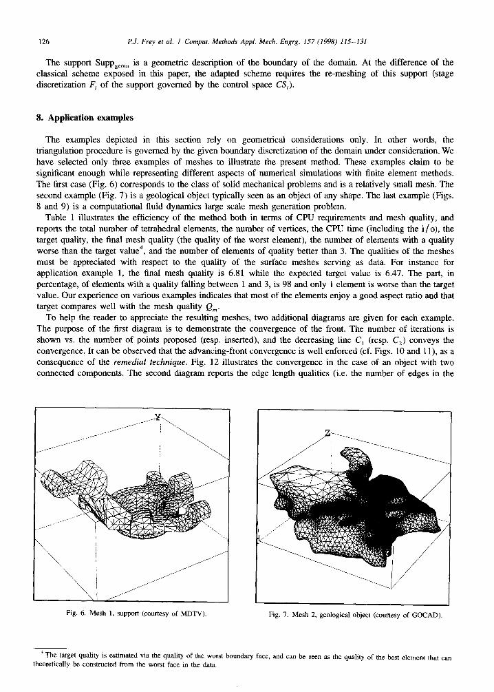
8. Application examples
The examples depicted in this section rely on geometrical considerations only. In other words, the
triangulation procedure is governed by the given boundary discretization of the domain under consideration. We
have selected only three examples of meshes to illustrate the present method. These examples claim to be significant enough while representing different aspects of numerical simulations with finite element methods.
The first case (Fig. 6) corresponds to the class of solid mechanical problems and is a relatively small mesh. The
second example (Fig. 7) is a geological object typically seen as an object of any shape. The last example (Figs. 8 and 9) is a computational fluid dynamics large scale mesh generation problem.
Table 1 illustrates the efficiency of the method both in terms of CPU requirements and mesh quality, and
reports the total number of tetrahedral elements, the number of vertices, the CPU time (including the i/o), the target quality, the final mesh quality (the quality of the worst element), the number of elements with a quality
worse than the target value4, and the number of elements of quality better than 3. The qualities of the meshes
must be appreciated with respect to the quality of the surface meshes serving as data. For instance for application example 1, the final mesh quality is 6.81 while the expected target value is 6.47. The part, in
percentage, of elements with a quality falling between 1 and 3, is 98 and only 1 element is worse than the target
value. Our experience on various examples indicates that most of the elements enjoy a good aspect ratio and that target compares well with the mesh quality Q,.
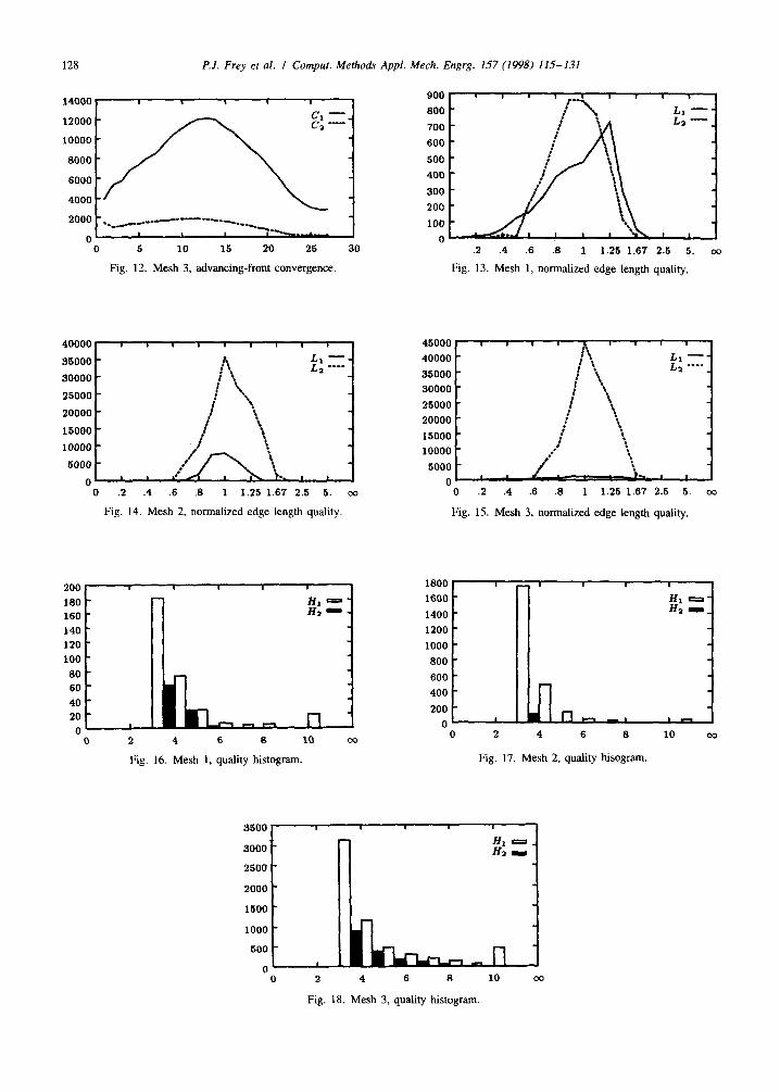
To help the reader to appreciate the resulting meshes, two additional diagrams are given for each example.
The purpose of the first diagram is to demonstrate the convergence of the front. The number of iterations is shown vs. the number of points proposed (resp. inserted), and the decreasing line C, (resp. C,) conveys the
convergence. It can be observed that the advancing-front convergence is well enforced (cf. Figs. 10 and 1 l), as a consequence of the remedial technique. Fig. 12 illustrates the convergence in the case of an object with two connected components. The second diagram reports the edge length qualities (i.e. the number of edges in the
Fig. 6. Mesh 1, support (courtesy of MDTV). Fig. 7. Mesh 2, geological object (courtesy of GOCAD).
It The target quality is estimated via the quality of the worst boundary face, and can be seen as the quality of the best element that can
theoretically be constructed from the worst face in the data.
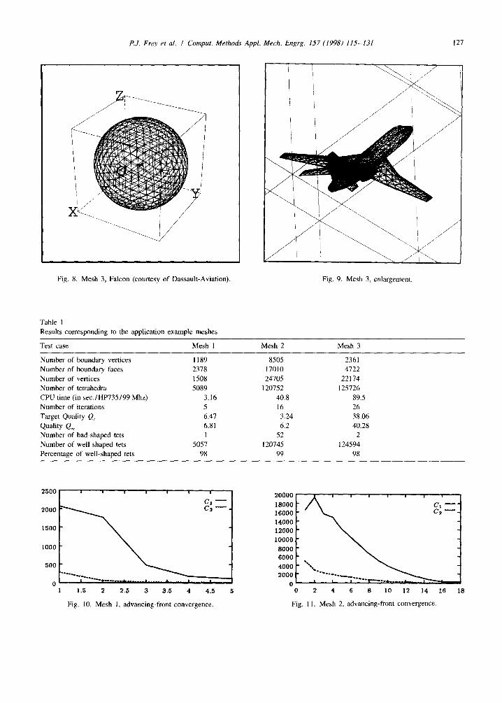
P.J. Frey et al. I Comput. Methods Appl. Mech. Engrg. 157 (1998) 115-131
Fig. 8. Mesh 3, Falcon (courtesy of Dassault-Aviation). Fig. 9. Mesh 3, enlargement.
Table 1 Results corresponding to the application example meshes
Test case Mesh I Mesh 2 Mesh 3
Number of boundary vertices 1189
Number of boundary faces 2378
Number of vertices 1508
Number of tetrahedra 5089
CPU time (in sec./HP735/99 Mhz :) 3.16
Number of iterations 5
Target Quality Q, 6.47
Quality Q, 6.81
Number of bad-shaped tets I Number of well-shaped tets 5057
Percentage of well-shaped tets 98
17010
24105
120752
40.8
16
3.24
6.2
52
120745
99
2361
4722
22174
125726
89.5
26
38.06
40.28
L
124594
98
2500 , I I I I I I
Cl - Ca --- -
1500 -
1000 -
500 -
1 1.5 2 2.5 3 3.5 4 4.5 5
Fig. IO. Mesh 1, advancing-front convergence.
12000 - 10000 -
8000 - 6000 -
0 2 4 6 8 10 12 14 16 18
Fig. 11. Mesh 2, advancing-front convergence.
128 P.J. Frey et al. I Comput. Methods Appl. Mech. Engrg. 157 (1998) 115-131
.‘_.c-.---------w._.__
0 5 10 15 20 25 30
Fig. 12. Mesh 3, advancing-front convergence.
40000‘ 1 1 1 I I 1 1 I I
35000 - .t Jh--
30000 - : ? La ----
25000 -
20000 -
15000 -
10000 -
5000 - 0 ._ , ,
0 .2 .4 .6 .8 1 1.25 1.67 2.5 5. CQ
Fig. 14. Mesh 2, normalized edge length quality.
200 I 1 I 1 1
180 - Hl- 160 - Hn - -
140 -
120 -
100 -
80 -
60 -
40 -
20 - I -mm r-l
0. 0 2 4 6 8 10 co
Fig. 16. Mesh 1, quality histogram.
800 -
700 -
600 -
500 -
400 -
300 -
200 -
.2 .4 .6 .8 1 1.25 1.67 2.5 5. 00
Fig. 13. Mesh 1, normalized edge length quality.
40000 -
35000 -
30000 -
25000 -
20000 -
15000 -
10000 -
0 .2 .4 .6 .8 1 1.25 1.67 2.5 5. co
Fig. 15. Mesh 3, normalized edge length quality.
1800
1600
1400
1200
1000
800
600
400
200
0 :II
0 2
-
m l-l, 1 I _
4 6 8 10 Co
Fig. 17. Mesh 2, quality hisogram.
v 3000 - HI -. Ha I
2500 -
2000 -
1500 -
1000 -
500 -
0 2 4 6 8 10
Fig. 18. Mesh 3, quality histogram.
P.J. Frey et al. I Comput. Methods Appl. Mech. Engrg. I57 (1998) 115-131 129
final mesh with a given edge length in the control space) for the initial surface triangulation (noted as 15,) and the final mesh (noted as L2). These diagrams (Figs. 13-15) show that the mesh is satisfactory in the control space and can be used for instance to perform finite element computations.
The histogram of mesh quality is given for each example before and after mesh optimization (lines H, and Hz, respectively). For a better understanding, the quality values better than 3 are not printed. The goal is to obtain an histogram skewed toward the left values and with as few as possible values worse than the target value Q,. Figs. 16-18 show the histogram quality.
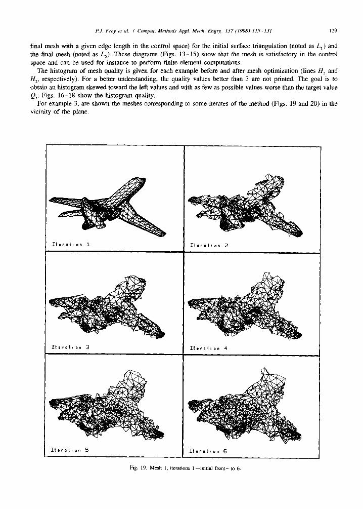
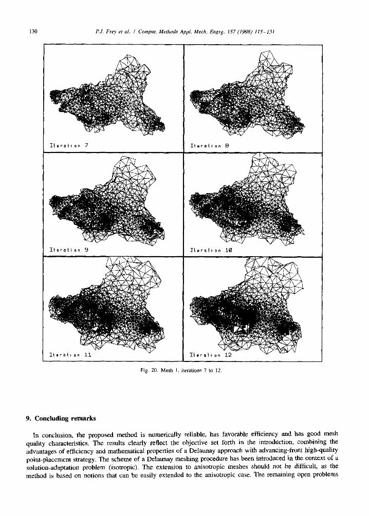
For example 3, are shown the meshes corresponding to some iterates of the method (Figs. 19 and 20) in the vicinity of the plane.
Iteratl on 3 IterOti on 4
IterOti on 5 Itoroti on 6
Fig. 19. Mesh 1, iterations l-initial front-to 6
P.J. Frey et al. I Comput. Methods Appl. Mech. Engrg. 157 (1998) 115-131
Fig. 20. Mesh 1, iterations 7 to 12
9. Concluding remarks
In conclusion, the proposed method is numerically reliable, has favorable efficiency and has good mesh quality characteristics. The results clearly reflect the objective set forth in the introduction, combining the advantages of efficiency and mathematical properties of a DeIaunay approach with advancing-front high-quality point-placement strategy. The scheme of a Delaunay meshing procedure has been introduced in the context of a solution-adaptation problem (isotropic). The extension to anisotropic meshes should not be difficult, as the method is based on notions that can be easily extended to the anisotropic case. The remaining open problems
P.J. Frey et al. I Comput. Methods Appl. Mech. Engrg. 157 (1998) 115-131 131
and extensions concern the implementation of the Delaunay kernel in the anisotropic case, the suitable definition
of the geometric support of the domain and the adapted remeshing of the surface with respect to the given
metric map (which constitutes a brand new stage with respect to the classical case).
References
[l] D.J. Mavriplis, Unstructured mesh generation and adaptivity, ICASE report #95-26, Apr 1995.
[2] S. Rebay, Efficient unstructured mesh generation by means of Delaunay triangulation and BowyerlWatson algorithm, 3rd Int. Conf. on
Numerical Grid Generation in Comp. Fluid Dyn., Barcelona, Spain, June 1991.
[3] J.D. Muller, P.L. Roe and H. Deconinck, A frontal approach for node generation in Delaunay triangulations, Unstructured grid methods
for advection dominated flows, VKI Lecture notes, pp. 9-l-9-7, AGARD Publication R-787, March 1992.
[4] D.L. Marcum and N.l? Weatherill, Unstructured grid generation using iterative point insertion and local reconnection, 41AA J. 33(9)
(1995) 1619-1625.
[5] M.L. Merriam, An efficient advancing front algorithm for Delaunay triangulation, AIAA paper 91-0792, January 1991.
[6] E. Briire de 1’Isle and P.L. George, Optimization of tetrahedral meshes, I. Babuska, W.D. Henshaw, J.E. Oliger, J.E. Flaherty, J.E.
Hopcroft and T. Tezduyar, eds., 75 (1995) 97-128.
[7] H. Borouchaki, P.L. George, F. Hecht, P Laug and E. Sahel, Delaunay mesh generation governed by metric specifications. Part I:
Algorithms, Finite Elements Anal. Des., 25 (1997) 61-83.
[8] PL. George, Automatic mesh generation. Application to Finite Element Methods (Wiley, 1991).
[9] F. Hermeline, Triangulation automatique d’un polyedre en dimension N, R.A.I.R.O. Analyse Num. 3 (1986) 231-246.
[lo] A. Bowyer, Computing Dirichlet tessellations, Comput. J. (1991) 162-169.
[l l] D.F. Watson, Computing the n-dimensional Delaunay tesselation with application toVoronoi’ polytopes, Comput. J. 24 (1981) 167-172.
[12] P.L. George and F. Hermeline, Delaunay’s mesh of a convex polyhedron in dimension d. Application for arbitrary polyhedra, Int. J.
Numer. Methods Engrg. 33 (1992) 975-995.
[13] H. Borouchaki, P.L. George and S.H. Lo, Optimal Delaunay point insertion, Int. J. Numer. Methods Engrg., 39 (1996) 3407-3437.
[14] T.J. Baker, Automatic mesh generation for complex three-dimensional regions using a constrained Delaunay triangulation, Engrg.
Comput. 5 (1989) 161-175.
[ 151 J. Peraire, J. Peiro, L. Formaggia, K. Morgan and O.C. Zienkiewicz, Finite element Euler computations in three dimensions, Int. J.
Numer. Methods Engrg. 26 (1988) 2135-2159.
[16] R. Lohner and P. Pa&h, Three-dimensional grid generation by the advancing-front method, Int. J. Numer. Methods Fluids 8 (1988)
1135-1149.
[17] D.J. Mavriplis, An advancing front Delaunay triangulation algorithm designed for robustness, ICASE report #92-49, October 1992.
[18] VN. Parthasarathy, C.M. Griachen and A.F. Hathaway, A comparison of tetrahedron quality measures, Finite Element Anal. Des. 15
(1993) 255-261.
[19] S.H. Lo, Automatic mesh generation and adaptation by using contours, Int. J. Numer. Methods Engrg. 31 (1991) 689-707.


![Using Transactions in Delaunay Mesh Generation2. Delaunay Mesh Generation A Delaunay mesh is a mesh over a set of points which satisfies the Delaunay property [4]. This property,](https://img.dokumen.tips/doc/110x75/5e78132d55760c30656ba589/using-transactions-in-delaunay-mesh-generation-2-delaunay-mesh-generation-a-delaunay.jpg)