Embed Size (px)
Citation preview
Chapter 34: Constraint Logic Programming over Finite Domains 445
34 Constraint Logic Programming over FiniteDomains
34.1 Introduction
The clp(FD) solver described in this chapter is an instance of the general Constraint LogicProgramming scheme introduced in [Jaffar & Michaylov 87]. This constraint domain isparticularly useful for modeling discrete optimization and verification problems such asscheduling, planning, packing, timetabling etc. The treatise [Van Hentenryck 89] is anexcellent exposition of the theoretical and practical framework behind constraint solving infinite domains, and summarizes the work up to 1989.
This solver has the following highlights:
• Two classes of constraints are handled internally: primitive constraints and globalconstraints.
• The constraints described in this chapter are automatically translated to conjunctionsof primitive and global library constraints.
• The truth value of a primitive constraint can be reflected into a 0/1-variable (reifica-tion).
• New primitive constraints can be added by writing so-called indexicals.
• New global constraints can be written in Prolog, by means of a programming interface.
This library fully supports multiple SICStus run-times in a process.
The rest of this chapter is organized as follows: How to load the solver and how to writesimple programs is explained in Section 34.2 [CLPFD Interface], page 446. A description ofall constraints that the solver provides is contained in Section 34.3 [Available Constraints],page 450. The predicates for searching for solution are documented in Section 34.4 [Enumer-ation Predicates], page 465. The predicates for getting execution statistics are documentedin Section 34.5 [Statistics Predicates], page 469. A few example programs are given inSection 34.10 [Example Programs], page 487. Finally, Section 34.11 [Syntax Summary],page 490 contains syntax rules for all expressions.
The following sections discuss advanced features and are probably only relevant to experi-enced users: How to control the amount of information presented in answers to queries isexplained in Section 34.6 [Answer Constraints], page 470. The solver’s execution mechanismand primitives are described in Section 34.7 [The Constraint System], page 470. How to addnew global constraints via a programming interface is described in Section 34.8 [DefiningGlobal Constraints], page 471. How to define new primitive constraints with indexicals isdescribed in Section 34.9 [Defining Primitive Constraints], page 479.
446 SICStus Prolog
34.1.1 Referencing this Software
When referring to this implementation of clp(FD) in publications, please use the followingreference:
Carlsson M., Ottosson G., Carlson B. An Open-Ended Finite Domain Con-straint Solver, Proc. Programming Languages: Implementations, Logics, andPrograms, 1997.
34.1.2 Acknowledgments
The first version of this solver was written as part of Key Hyckenberg’s MSc thesis in 1995,with contributions from Greger Ottosson at the Computing Science Department, UppsalaUniversity. The code was later rewritten by Mats Carlsson. Peter Szeredi contributedmaterial for this manual chapter.
The development of this software was supported by the Swedish National Board for Techni-cal and Industrial Development (NUTEK) under the auspices of Advanced Software Tech-nology (ASTEC) Center of Competence at Uppsala University.
We include a collection of examples, some of which have been distributed with the INRIAimplementation of clp(FD) [Diaz & Codognet 93].
34.2 Solver Interface
The solver is available as a library module and can be loaded with a query
:- use_module(library(clpfd)).
The solver contains predicates for checking the consistency and entailment of finite domainconstraints, as well as solving for solution values for your problem variables.
In the context of this constraint solver, a finite domain is a subset of small integers, and afinite domain constraint denotes a relation over a tuple of small integers. Hence, only smallintegers and unbound variables are allowed in finite domain constraints.
All domain variables, i.e. variables that occur as arguments to finite domain constraintsget associated with a finite domain, either explicitly declared by the program, or implicitlyimposed by the constraint solver. Temporarily, the domain of a variable may actually beinfinite, if it does not have a finite lower or upper bound. If during the computation avariable receives a new lower or upper bound that cannot be represented as a small integer,an overflow condition is issued. This is expressed as silent failure or as a representationerror, subject to the overflow option of fd_flag/3.
Chapter 34: Constraint Logic Programming over Finite Domains 447
The domain of all variables gets narrower and narrower as more constraints are added. Ifa domain becomes empty, the accumulated constraints are unsatisfiable, and the currentcomputation branch fails. At the end of a successful computation, all domains have usuallybecome singletons, i.e. the domain variables have become assigned.
The domains do not become singletons automatically. Usually, it takes some amount ofsearch to find an assignment that satisfies all constraints. It is the programmer’s responsi-bility to do so. If some domain variables are left unassigned in a computation, the garbagecollector will preserve all constraint data that is attached to them.
Please note: the behavior of the predicates assert/1, findall/3, raise_exception/1
and friends is undefined on non-ground terms containing domain variables. If you needto apply these operations to a term containing domain variables, fd_copy_term/3 may beused to decompose the term into a template and a symbolic representation of the relevantconstraints.
The heart of the constraint solver is a scheduler for indexicals [Van Hentenryck et al. 92]and global constraints. Both entities act as coroutines performing incremental constraintsolving or entailment checking. They wake up by changes in the domains of its arguments.All constraints provided by this package are implemented as indexicals or global constraints.New constraints can be defined by the user.
Indexicals are reactive functional rules, which take part in the solver’s basic constraintsolving algorithm, whereas each global constraint is associated with its particular constraintsolving algorithm. The solver maintains two scheduling queues, giving priority to the queueof indexicals.
The feasibility of integrating the indexical approach with a Prolog based on the WAM wasclearly demonstrated by Diaz’s clp(FD) implementation [Diaz & Codognet 93], one of thefastest finite domains solvers around.
34.2.1 Posting Constraints
A constraint is called as any other Prolog predicate. When called, the constraint is postedto the store. For example:
| ?- X in 1..5, Y in 2..8, X+Y #= T.
X in 1..5,
Y in 2..8,
T in 3..13
| ?- X in 1..5, T in 3..13, X+Y #= T.
X in 1..5,
T in 3..13,
Y in -2..12

448 SICStus Prolog
Note that the answer constraint shows the domains of nonground query variables, but notany constraints that may be attached to them.
34.2.2 A Constraint Satisfaction Problem
Constraint satisfaction problems (CSPs) are a major class of problems for which this solveris ideally suited. In a CSP, the goal is to pick values from pre-defined domains for certainvariables so that the given constraints on the variables are all satisfied.
As a simple CSP example, let us consider the Send More Money puzzle. In this problem,the variables are the letters S, E, N, D, M, O, R, and Y. Each letter represents a digitbetween 0 and 9. The problem is to assign a value to each digit, such that SEND + MOREequals MONEY.
A program that solves the puzzle is given below. The program contains the typical threesteps of a clp(FD) program:
1. declare the domains of the variables
2. post the problem constraints
3. look for a feasible solution via backtrack search, or look for an optimal solution viabranch-and-bound search
Sometimes, an extra step precedes the search for a solution: the posting of surrogate con-straints to break symmetries or to otherwise help prune the search space. No surrogateconstraints are used in this example.
The domains of this puzzle are stated via the domain/3 goal and by requiring that S and Mbe greater than zero. The two problem constraint of this puzzle are the equation (sum/8)and the constraint that all letters take distinct values (all_different/1). Finally, thebacktrack search is performed by labeling/2. Different search strategies can be encodedin the Type parameter. In the example query, the default search strategy is used (select theleftmost variable, try values in ascending order).

Chapter 34: Constraint Logic Programming over Finite Domains 449
:- use_module(library(clpfd)).
mm([S,E,N,D,M,O,R,Y], Type) :-
domain([S,E,N,D,M,O,R,Y], 0, 9), % step 1
S#>0, M#>0,
all_different([S,E,N,D,M,O,R,Y]), % step 2
sum(S,E,N,D,M,O,R,Y),
labeling(Type, [S,E,N,D,M,O,R,Y]). % step 3
sum(S, E, N, D, M, O, R, Y) :-
1000*S + 100*E + 10*N + D
+ 1000*M + 100*O + 10*R + E
#= 10000*M + 1000*O + 100*N + 10*E + Y.
| ?- mm([S,E,N,D,M,O,R,Y], []).
D = 7,
E = 5,
M = 1,
N = 6,
O = 0,
R = 8,
S = 9,
Y = 2
34.2.3 Reified Constraints
Instead of merely posting constraints it is often useful to reflect its truth value into a 0/1-variable B, so that:
• the constraint is posted if B is set to 1
• the negation of the constraint is posted if B is set to 0
• B is set to 1 if the constraint becomes entailed
• B is set to 0 if the constraint becomes disentailed
This mechanism is known as reification. Several frequently used operations can be definedin terms of reified constraints, such as blocking implication [Saraswat 90] and the cardinalityoperator [Van Hentenryck & Deville 91], to name a few. A reified constraint is written:
| ?- Constraint #<=> B.
where Constraint is reifiable. As an example of a constraint that uses reification, considerexactly(X,L,N), which is true if X occurs exactly N times in the list L. It can be definedthus:
450 SICStus Prolog
exactly(_, [], 0).
exactly(X, [Y|L], N) :-
X #= Y #<=> B,
N #= M+B,
exactly(X, L, M).
34.3 Available Constraints
This section describes the classes of constraints that can be used with this solver.
34.3.1 Arithmetic Constraints
?Expr RelOp ?Expr
defines an arithmetic constraint. The syntax for Expr and RelOp is defined bya grammar (see Section 34.11.2 [Syntax of Arithmetic Expressions], page 492).Note that the expressions are not restricted to being linear. Constraints overnon-linear expressions, however, will usually yield less constraint propagationthan constraints over linear expressions.
Arithmetic constraints can be reified as e.g.:
| ?- X in 1..2, Y in 3..5, X#=<Y #<=> B.
B = 1,
X in 1..2,
Y in 3..5
Linear arithmetic constraints, except equalities, maintain interval-consistency and their rei-fied versions detect interval-entailment and -disentailment; see Section 34.7 [The ConstraintSystem], page 470.
The following constraints are among the library constraints that general arithmetic con-straints compile to. They express a relation between a sum or a scalar product and avalue, using a dedicated algorithm, which avoids creating any temporary variables holdingintermediate values. If you are computing a sum or a scalar product, it can be much moreefficient to compute lists of coefficients and variables and post a single sum or scalar productconstraint than to post a sequence of elementary constraints.
sum(+Xs, +RelOp, ?Value)
where Xs is a list of integers or domain variables, RelOp is a relational symbolas above, and Value is an integer or a domain variable. True if Xs RelOp Value.Cannot be reified.
scalar_product(+Coeffs, +Xs, +RelOp, ?Value)
where Coeffs is a list of length n of integers, Xs is a list of length n of integers ordomain variables, RelOp is a relational symbol as above, and Value is an integeror a domain variable. True if Coeffs*Xs RelOp Value. Cannot be reified.

Chapter 34: Constraint Logic Programming over Finite Domains 451
The following constraint is a special case of scalar_product/4 where RelOp is #=, andwhich is domain-consistent in the Xs:
knapsack(+Coeffs, +Xs, ?Value)
where Coeffs is a list of length n of non-negative integers, Xs is a list of length nof non-negative integers or domain variables, and Value is an integer or a domainvariable. Any domain variables must have finite bounds. True if Coeffs*Xs =Value. Cannot be reified.
34.3.2 Membership Constraints
domain(+Variables, +Min, +Max)
where Variables is a list of domain variables or integers, Min is an integer orthe atom inf (minus infinity), and Max is an integer or the atom sup (plusinfinity). True if the variables all are elements of the range Min..Max. Cannotbe reified.
?X in +Range
defines a membership constraint. X is an integer or a domain variable and Rangeis a ConstantRange (see Section 34.11.1 [Syntax of Indexicals], page 491). Trueif X is an element of the range.
?X in_set +FDSet
defines a membership constraint. X is an integer or a domain variable andFDSet is an FD set term (see Section 34.8.3 [FD Set Operations], page 475).True if X is an element of the FD set.
in/2 and in_set/2 constraints can be reified. They maintain domain-consistency andtheir reified versions detect domain-entailment and -disentailment; see Section 34.7 [TheConstraint System], page 470.
34.3.3 Propositional Constraints
Propositional combinators can be used to combine reifiable constraints into propositionalformulae over such constraints. Such formulae are goal expanded by the system into se-quences of reified constraints and arithmetic constraints. For example,
X #= 4 #\/ Y #= 6
expresses the disjunction of two equality constraints.
The leaves of propositional formulae can be reifiable constraints, the constants 0 and 1,or 0/1-variables. New primitive, reifiable constraints can be defined with indexicals asdescribed in Section 34.9 [Defining Primitive Constraints], page 479. The following propo-sitional combinators are available:
#\ :Q

452 SICStus Prolog
True if the constraint Q is false.
:P #/\ :Q
True if the constraints P and Q are both true.
:P #\ :Q
True if exactly one of the constraints P and Q is true.
:P #\/ :Q
True if at least one of the constraints P and Q is true.
:P #=> :Q
:Q #<= :P
True if the constraint Q is true or the constraint P is false.
:P #<=> :Q
True if the constraints P and Q are both true or both false.
Note that the reification scheme introduced in Section 34.2.3 [Reified Constraints], page 449is a special case of a propositional constraint.
34.3.4 Combinatorial Constraints
The constraints listed here are sometimes called symbolic constraints. They are currentlynot reifiable. Unless documented otherwise, they maintain (at most) interval-consistencyin their arguments; see Section 34.7 [The Constraint System], page 470.
count(+Val,+List,+RelOp,?Count)
where Val is an integer, List is a list of integers or domain variables, Countan integer or a domain variable, and RelOp is a relational symbol as in Sec-tion 34.3.1 [Arithmetic Constraints], page 450. True if N is the number ofelements of List that are equal to Val and N RelOp Count. Thus, count/4 isa generalization of exactly/3 (not an exported constraint), which was used inan example earlier.
count/4 maintains domain-consistency, but in practice, the following constraintis a better alternative.
global_cardinality(+Xs,+Vals)
global_cardinality(+Xs,+Vals,+Options)
where Xs = [X1, . . . , Xd] is a list of integers or domain variables, and Vals =[K1 − V1, . . . ,Kn − Vn] is a list of pairs where each key Ki is a unique integerand Vi is a domain variable or an integer. True if every element of Xs is equalto some key and for each pair Ki − Vi, exactly Vi elements of Xs are equal toKi.
If either Xs or Vals is ground, and in many other special cases, global_
cardinality/[2,3] maintains domain-consistency, but generally, interval-consistency cannot be guaranteed. A domain-consistency algorithm [Regin 96]is used, roughly linear in the total size of the domains.

Chapter 34: Constraint Logic Programming over Finite Domains 453
Options is a list of zero or more of the following:
cost(Cost,Matrix)
A cost is associated with the constraint and reflected into the do-main variable Cost. Matrix should be a d×n matrix, represented asa list of d lists, each of length n. Assume that each Xi equals Kpi
.The cost of the constraint is then Matrix [1, p1]+ · · ·+Matrix [d, pd].
With this option, a domain-consistency algorithm [Regin 99] isused, the complexity of which is roughly O(d(m + n log n)) wherem is the total size of the domains.
element(?X,+List,?Y)
where X and Y are integers or domain variables and List is a list of integersor domain variables. True if the X:th element of List is Y. Operationally, thedomains of X and Y are constrained so that for every element in the domain ofX, there is a compatible element in the domain of Y, and vice versa.
This constraint uses an optimized algorithm for the special case where List isground.
element/3 maintains domain-consistency in X and interval-consistency in Listand Y.
relation(?X,+MapList,?Y)
where X and Y are integers or domain variables and MapList is a list of in-teger-ConstantRange pairs, where the integer keys occur uniquely (see Sec-tion 34.11.1 [Syntax of Indexicals], page 491). True if MapList contains a pairX-R and Y is in the range denoted by R.
Operationally, the domains of X and Y are constrained so that for every elementin the domain of X, there is a compatible element in the domain of Y, and viceversa.
If MapList is not ground, the constraint must be wrapped in call/1 to postponegoal expansion until runtime.
An arbitrary binary constraint can be defined with relation/3. relation/3
is implemented in terms of the following, more general constraint, with whicharbitrary relations can be defined compactly:
case(+Template, +Tuples, +Dag)
case(+Template, +Tuples, +Dag, +Options)
Template is an arbitrary non-ground Prolog term. Its variables are merelyplace-holders; they should not occur outside the constraint nor inside Tuples.
Tuples is a list of terms of the same shape as Template. They should not shareany variables with Template.
Dag is a list of nodes of the form node(ID,X,Successors), where X is a place-holder variable. The set of all X should equal the set of variables in Template.The first node in the list is the root node. Let rootID denote its ID.
Nodes are either internal nodes or leaf nodes. In the former case, Successorsis a list of terms (Min..Max)-ID2, where the ID2 refers to a child node. Inthe latter case, Successors is a list of terms (Min..Max). In both cases, the(Min..Max) should form disjoint intervals.

454 SICStus Prolog
ID is a unique, integer identifier of a node.
Each path from the root node to a leaf node corresponds to one set of tuplesadmitted by the relation expressed by the constraint. Each variable in Templateshould occur exactly once on each path, and there must not be any cycles.
Options is a list of zero or more of the following. It can be used to control thewaking and pruning conditions of the constraint, as well as to identify the leafnodes reached by the tuples:
leaves(TLeaf,Leaves)
TLeaf is a place-holder variable. Leaves is a list of variables of thesame length as Tuples. This option effectively extends the relationby one argument, corresponding to the ID of the leaf node reachedby a particular tuple.
on(Spec) Specifies how eagerly the constraint should react to domain changesof X.
prune(Spec)
Specifies the extent to which the constraint should prune the do-main of X.
Spec is one of the following, where X is a place-holder variable occurring inTemplate or equal to TLeaf:
dom(X) wake up when the domain of X has changed, resp. perform fullpruning on X. This is the default for all variables mentioned in theconstraint.
min(X) wake up when the lower bound of X has changed, resp. prune onlythe lower bound of X.
max(X) wake up when the upper bound of X has changed, resp. prune onlythe upper bound of X.
minmax(X)
wake up when the lower or upper bound of X has changed, resp.prune only the bounds of X.
val(X) wake up when X has become ground, resp. only prune X when itsdomain has been narrowed to a singleton.
none(X) ignore domain changes of X, resp. never prune X.
The constraint holds if path(rootID,Tuple,Leaf) holds for each Tuple in Tuplesand Leaf is the corresponding element of Leaves if given (otherwise, Leaf is afree variable).
path(ID,Tuple,Leaf) holds if Dag contains a term node(ID,Var,Successors),Var is the unique k:th element of Template, i is the k:th element of Tuple, and:
• The node is an internal node, and
1. Successors contains a term (Min..Max)-Child,
2. Min ≤ i ≤ Max , and
3. path(Child,Tuple,Leaf) holds; or
Chapter 34: Constraint Logic Programming over Finite Domains 455
• The node is a leaf node, and
1. Successors contains a term (Min..Max),
2. Min ≤ i ≤ Max , and Leaf = ID.
For example, recall that element(X,L,Y) wakes up when the domain of X orthe lower or upper bound of Y has changed, performs full pruning of X, butonly prunes the bounds of Y. The following two constraints:
element(X, [1,1,1,1,2,2,2,2], Y),
element(X, [10,10,20,20,10,10,30,30], Z)
can be replaced by the following single constraint, which is equivalent declara-tively as well as wrt. pruning and waking. The fourth argument illustrates theleaf feature:
elts(X, Y, Z, L) :-
case(f(A,B,C), [f(X,Y,Z)],
[node(0, A,[(1..2)-1,(3..4)-2,(5..6)-3,(7..8)-4]),
node(1, B,[(1..1)-5]),
node(2, B,[(1..1)-6]),
node(3, B,[(2..2)-5]),
node(4, B,[(2..2)-7]),
node(5, C,[(10..10)]),
node(6, C,[(20..20)]),
node(7, C,[(30..30)])],
[on(dom(A)),on(minmax(B)),on(minmax(C)),
prune(dom(A)),prune(minmax(B)),prune(minmax(C)),
leaves(_,[L])]).
The DAG of the previous example has the following shape:

456 SICStus Prolog
DAG corresponding to elts/4
A couple of sample queries:
Chapter 34: Constraint Logic Programming over Finite Domains 457
| ?- elts(X, Y, Z, L).
L in 5..7,
X in 1..8,
Y in 1..2,
Z in 10..30
| ?- elts(X, Y, Z, L), Z #>= 15.
L in 6..7,
X in(3..4)\/(7..8),
Y in 1..2,
Z in 20..30
| ?- elts(X, Y, Z, L), Y = 1.
Y = 1,
L in 5..6,
X in 1..4,
Z in 10..20
| ?- elts(X, Y, Z, L), L = 5.
Z = 10,
X in(1..2)\/(5..6),
Y in 1..2
all_different(+Variables)
all_different(+Variables, +Options)
all_distinct(+Variables)
all_distinct(+Variables, +Options)
where Variables is a list of domain variables with bounded domains or integers.Each variable is constrained to take a value that is unique among the variables.Declaratively, this is equivalent to an inequality constraint for each pair ofvariables.
Options is a list of zero or more of the following:
on(On) How eagerly to wake up the constraint. One of:
dom (the defaultfor all_distinct/[1,2] and assignment/[2,3]), towake up when the domain of a variable is changed;
min to wake up when the lower bound of a domain ischanged;
max to wake up when the upper bound of a domain ischanged;
minmax to wake up when some bound of a domain is changed;
val (the default for all_different/[1,2]), to wake upwhen a variable becomes ground.

458 SICStus Prolog
consistency(Cons)
Which algorithm to use, one of:
global The default for all_distinct/[1,2] andassignment/[2,3]. A domain-consistency algorithm[Regin 94] is used, roughly linear in the total size ofthe domains.
local The default for all_different/[1,2]. An algorithmachieving exactly the same pruning as a set of pair-wise inequality constraints is used, roughly linear inthe number of variables.
bound An interval-consistency algorithm [Mehlhorn 00] isused. This algorithm is nearly linear in the numberof variables and values.
The following is a constraint over two lists of length n of variables. Each variable is con-strained to take a value in [1, n] that is unique for its list. Furthermore, the lists are dualin a sense described below.
assignment(+Xs, +Ys)
assignment(+Xs, +Ys, +Options)
where Xs = [X1, . . . , Xn] and Ys = [Y1, . . . , Yn] are lists of domain variables orintegers. True if all Xi, Yi ∈ [1, n] and Xi = j ≡ Yj = i.
Options is a list of zero or more of the following, where Boolean must be true
or false (false is the default):
on(On) Same meaning as for all_different/2.
consistency(Cons)
Same meaning as for all_different/2.
circuit(Boolean)
If true, circuit(Xs,Ys) must hold for the constraint to be true.
cost(Cost,Matrix)
A cost is associated with the constraint and reflected into the do-main variable Cost. Matrix should be an n×n matrix, representedas a list of lists. The cost of the constraint is Matrix [1, X1] + · · ·+Matrix [n, Xn].
With this option, a domain-consistency algorithm [Sellmann 02] isused, the complexity of which is roughly O(n(m + n log n)) wherem is the total size of the domains.
The following constraint can be thought of as constraining n nodes in a graph to form aHamiltonian circuit. The nodes are numbered from 1 to n. The circuit starts in node 1,visits each node, and returns to the origin.

Chapter 34: Constraint Logic Programming over Finite Domains 459
circuit(+Succ)
circuit(+Succ, +Pred)
where Succ is a list of length n of domain variables or integers. The i:th elementof Succ (Pred) is the successor (predecessor) of i in the graph. True if the valuesform a Hamiltonian circuit.
The following constraint can be thought of as constraining n tasks, each with a start timeSj and a duration Dj, so that no tasks ever overlap. The tasks can be seen as competingfor some exclusive resource.
serialized(+Starts,+Durations)
serialized(+Starts,+Durations,+Options)
where Starts = [S1, . . . , Sn] and Durations = [D1, . . . , Dn] are lists of domainvariables with finite bounds or integers. Durations must be non-negative. Trueif Starts and Durations denote a set of non-overlapping tasks, i.e.:
∀i, j ∈ [1, n] ∧ i < j :
Si + Di ≤ Sj∨
Sj + Dj ≤ Si∨
Di = 0∨
Dj = 0
Theserialized/[2,3] constraint is merely a special case of cumulative/[4,5]
(see below).
Options is a list of zero or more of the following, where Boolean must be true
or false (false is the default, except for the bounds_only option):
precedences(Ps)
Ps encodes a set of precedence constraints to apply to the tasks.Ps should be a list of terms of one of the forms:
• d(i, j, k), where i and j should be task numbers, and k shouldbe a positive integer or sup, denoting:
{
Si + k ≤ Sj ∨ Sj ≤ Si, if k is an integer
Sj ≤ Si, if k is sup
• i-j in r, where i and j should be task numbers, and r shouldbe a ConstantRange (see Section 34.11.1 [Syntax of Indexicals],page 491), denoting:
Si − Sj = Dij ∧ Dij ∈ r
resource(R)
R is unified with a term that can be passed to order_resource/2
(see Section 34.4 [Enumeration Predicates], page 465) in order tofind a consistent ordering of the tasks.
460 SICStus Prolog
path_consistency(Boolean)
if true, a redundant path-consistency algorithm will be used insidethe constraint in an attempt to improve the pruning.
static_sets(Boolean)
if true, a redundant algorithm will be used, which reasons aboutthe set of tasks that must precede (be preceded by) a given task,in an attempt to tighten the lower (upper) bound of a given startvariable.
edge_finder(Boolean)
if true, a redundant algorithm will be used, which attempts toidentify tasks that necessarily precede or are preceded by some setof tasks.
decomposition(Boolean)
if true, an attempt is made to decompose the constraint each timeit is resumed.
bounds_only(Boolean)
if true, the constraints will only prune the bounds of the Si vari-ables, and not inside the domains.
Whether it’s worthwhile to switch on any of the latter five options is highlyproblem dependent.
serialized/3 can model a set of tasks to be serialized with sequence-dependentsetup times. For example, the following constraint models three tasks, all withduration 5, where task 1 must precede task 2 and task 3 must either completebefore task 2 or start at least 10 time units after task 2 started:
?- domain([S1,S2,S3], 0, 20),
serialized([S1,S2,S3], [5,5,5],
[precedences([d(2,1,sup),d(2,3,10)])]).
S1 in 0..15,
S2 in 5..20,
S3 in 0..20
The bounds of S1 and S2 changed because of the precedence constraint. SettingS2 to 5 will propagate S1=0 and S3 in 15..20.
The following constraint can be thought of as constraining n tasks to be placed in timeand on m machines. Each machine has a resource limit, which is interpreted as a lower orupper bound on the total amount of resource used on that machine at any point in timethat intersects with some task.
A task is represented by a term task(Oi, Di, Ei,Hi,Mi) where Oi is the start time, Di theduration, Ei the end time, Hi the resource consumption, and Mi a machine identifier.
A machine is represented by a term machine(Mj, Lj) where Mj is the identifier and Lj isthe resource limit of the machine.

Chapter 34: Constraint Logic Programming over Finite Domains 461
All fields are domain variables with bounded domains, or integers. Lj must be an integer.Di must be non-negative, but Hi may be either positive or negative. Negative resourceconsumption is interpreted as resource production.
cumulatives(+Tasks,+Machines)
cumulatives(+Tasks,+Machines,+Options)
Options is a list of zero or more of the following, where Boolean must be true
or false (false is the default):
bound(B) If lower (the default), each resource limit is treated as a lowerbound. If upper, each resource limit is treated as an upper bound.
prune(P) If all (the default), the constraint will try to prune as many vari-ables as possible. If next, only variables that occur in the firstnon-ground task term (wrt. the order given when the constraintwas posted) can be pruned.
generalization(Boolean)
If true, extra reasoning based on assumptions on machine assign-ment will be done to infer more.
task_intervals(Boolean)
If true, extra global reasoning will be performed in an attempt toinfer more.
The following constraint can be thought of as constraining n tasks, each with a start timeSj, a duration Dj, and a resource amount Rj, so that the total resource consumption doesnot exceed Limit at any time:
cumulative(+Starts,+Durations,+Resources,?Limit)
cumulative(+Starts,+Durations,+Resources,?Limit,+Options)
where Starts = [S1, . . . , Sn], Durations = [D1, . . . , Dn], and Resource =[R1, . . . , Rn] are lists of domain variables with finite bounds or integers, andLimit is a domain variable with finite bounds or an integer. Durations, Re-sources and Limit must be non-negative. Let:
a = min(S1, . . . , Sn)
b = max(S1 + D1, . . . , Sn + Dn)
Rij =
{
Rj, if Sj ≤ i < Sj + Dj
0, otherwise
The constraint holds if:
∀a ≤ i < b : Ri1 + · · · + Rin ≤ Limit
If given, Options should be of the same form as in serialized/3, except theresource(R) option is not useful in cumulative/5.
The cumulative/4 constraint is due to Aggoun and Beldiceanu [Aggoun &Beldiceanu 93].
462 SICStus Prolog
The following constraint captures the relation between a list of values, a list of the valuesin ascending order, and their positions in the original list:
sorting(+Xs,+Ps,+Ys)
where Xs = [X1, . . . , Xn], Ps = [P1, . . . , Pn], and Ys = [Y1, . . . , Yn] are lists ofdomain variables or integers. The constraint holds if the following are true:
• Ys is in ascending order.
• Ps is a permutation of [1, n].
• ∀i ∈ [1, n] : Xi = YPi
In practice, the underlying algorithm [Mehlhorn 00] is likely to achieve interval-consistency, and is guaranteed to do so if Ps is ground or completely free.
The following constraints model a set or lines or rectangles, respectively, so that no pair ofobjects overlap:
disjoint1(+Lines)
disjoint1(+Lines,+Options)
where Lines is a list of terms F (Sj, Dj) or F (Sj, Dj, Tj), Sj and Dj are domainvariables with finite bounds or integers denoting the origin and length of line j
respectively, F is any functor, and the optional Tj is an atomic term denotingthe type of the line. Tj defaults to 0 (zero).
Options is a list of zero or more of the following, where Boolean must be true
or false (false is the default):
decomposition(Boolean)
if true, an attempt is made to decompose the constraint each timeit is resumed.
global(Boolean)
if true, a redundant algorithm using global reasoning is used toachieve more complete pruning.
wrap(Min,Max)
If used, the space in which the lines are placed should be thoughtof as a circle where positions Min and Max coincide, where Minand Max should be integers. That is, the space wraps around.Furthermore, this option forces the domains of the origin variablesto be inside [Min,Max-1].
margin(T1,T2,D)
This option imposes a minimal distance D between the end point ofany line of type T1 and the origin of any line of type T2. D shouldbe a positive integer or sup. If sup is used, all lines of type T2 mustbe placed before any line of type T1.
This option interacts with the wrap/2 option in the sense thatdistances are counted with possible wrap-around, and the distancebetween any end point and origin is always finite.
Chapter 34: Constraint Logic Programming over Finite Domains 463
The file library(’clpfd/examples/bridge.pl’) contains an example wheredisjoint1/2 is used for scheduling non-overlapping tasks.
disjoint2(+Rectangles)
disjoint2(+Rectangles,+Options)
where Rectangles is a list of terms F (Sj1 , Dj1 , Sj2 , Dj2) orF (Sj1 , Dj1 , Sj2 , Dj2 , Tj), Sj1 and Dj1 are domain variables with finite boundsor integers denoting the origin and size of rectangle j in the X dimension, Sj2
and Dj2 are the values for the Y dimension, F is any functor, and the optionalTj is an atomic term denoting the type of the rectangle. Tj defaults to 0 (zero).
Options is a list of zero or more of the following, where Boolean must be true
or false (false is the default):
decomposition(Boolean)
If true, an attempt is made to decompose the constraint each timeit is resumed.
global(Boolean)
If true, a redundant algorithm using global reasoning is used toachieve more complete pruning.
wrap(Min1,Max1,Min2,Max2)
Min1 and Max1 should be either integers or the atoms inf and sup
respectively. If they are integers, the space in which the rectanglesare placed should be thought of as a cylinder wrapping around the Xdimension where positions Min1 and Max1 coincide. Furthermore,this option forces the domains of the Sj1 variables to be inside[Min1,Max1-1].
Min2 and Max2 should be either integers or the atoms inf and sup
respectively. If they are integers, the space in which the rectanglesare placed should be thought of as a cylinder wrapping around the Ydimension where positions Min2 and Max2 coincide. Furthermore,this option forces the domains of the Sj2 variables to be inside[Min2,Max2-1].
If all four are integers, the space is a toroid wrapping around bothdimensions.
margin(T1,T2,D1,D2)
This option imposes minimal distances D1 in the X dimension andD2 in the Y dimension between the end point of any rectangle oftype T1 and the origin of any rectangle of type T2. D1 and D2
should be positive integers or sup. If sup is used, all rectanglesof type T2 must be placed before any rectangle of type T1 in therelevant dimension.
This option interacts with the wrap/4 option in the sense thatdistances are counted with possible wrap-around, and the distancebetween any end point and origin is always finite.
The file library(’clpfd/examples/squares.pl’) contains an example wheredisjoint2/2 is used for tiling squares.

464 SICStus Prolog
synchronization(Boolean)
Let the assignment dimension and the temporal dimension denote the two di-mensions, no matter which is the X and which is the Y dimension. If Booleanis true, a redundant algorithm is used to achieve more complete pruning forthe following case:
• All rectangles have size 1 in the assignment dimension.
• Some rectangles have the same origin and size in the temporal dimension,and that origin is not yet fixed.
The following example shows an artificial placement problem involving 25 rect-angles including four groups of rectangles whose left and right borders mustbe aligned. If Synch is true, it can be solved with first-fail labeling in 23backtracks. If Synch is false, 60 million backtracks do not suffice to solve it.
ex([O1,Y1a,Y1b,Y1c,
O2,Y2a,Y2b,Y2c,Y2d,
O3,Y3a,Y3b,Y3c,Y3d,
O4,Y4a,Y4b,Y4c],
Synch) :-
domain([Y1a,Y1b,Y1c,
Y2a,Y2b,Y2c,Y2d,
Y3a,Y3b,Y3c,Y3d,
Y4a,Y4b,Y4c], 1, 5),
O1 in 1..28,
O2 in 1..26,
O3 in 1..22,
O4 in 1..25,
disjoint2([t(1,1,5,1), t(20,4,5,1),
t(1,1,4,1), t(14,4,4,1),
t(1,2,3,1), t(24,2,3,1),
t(1,2,2,1), t(21,1,2,1),
t(1,3,1,1), t(14,2,1,1),
t(O1,3,Y1a,1),
t(O1,3,Y1b,1),
t(O1,3,Y1c,1),
t(O2,5,Y2a,1),
t(O2,5,Y2b,1),
t(O2,5,Y2c,1),
t(O2,5,Y2d,1),
t(O3,9,Y3a,1),
t(O3,9,Y3b,1),
t(O3,9,Y3c,1),
t(O3,9,Y3d,1),
t(O4,6,Y4a,1),
t(O4,6,Y4b,1),
t(O4,6,Y4c,1)],
[synchronization(Synch)]).

Chapter 34: Constraint Logic Programming over Finite Domains 465
The following constraints express the fact that several vectors of domain variables are inascending lexicographic order:
lex_chain(+Vectors)
lex_chain(+Vectors,+Options)
where Vectors is a list of vectors (lists) of domain variables with finite bounds orintegers. The constraint holds if Vectors are in ascending lexicographic order.
Options is a list of zero or more of the following:
op(Op) If Op is the atom #=< (the default), the constraints holds if Vectorsare in non-descending lexicographic order. If Op is the atom #<, theconstraints holds if Vectors are in strictly ascending lexicographicorder.
among(Least,Most,Values)
If given, Least and Most should be integers such that 0 ≤ Least ≤Most and Values should be a list of distinct integers. This optionimposes the additional constraint on each vector in Vectors that atleast Least and at most Most elements should belong to Values.
In the absence of an among/3 option, the underlying algorithm [Carlsson &Beldiceanu 02] guarantees domain-consistency.
34.3.5 User-Defined Constraints
New, primitive constraints can be added defined by the user on two different levels. On ahigher level, constraints can be defined using the global constraint programming interface;see Section 34.8 [Defining Global Constraints], page 471. Such constraints can embodyspecialized algorithms and use the full power of Prolog. They cannot be reified.
On a lower level, new primitive constraints can be defined with indexicals. In this case,they take part in the basic constraint solving algorithm and express custom designed rulesfor special cases of the overall local propagation scheme. Such constraints are called FDpredicates; see Section 34.9 [Defining Primitive Constraints], page 479. They can optionallybe reified.
34.4 Enumeration Predicates
As is usually the case with finite domain constraint solvers, this solver is not complete.That is, it does not ensure that the set of posted constraints is satisfiable. One must resortto search (enumeration) to check satisfiability and get particular solutions.
The following predicates provide several variants of search:

466 SICStus Prolog
indomain(?X)
where X is a domain variable with a bounded domain or an integer. Assigns,in increasing order via backtracking, a feasible value to X.
labeling(:Options, +Variables)
where Variables is a list of domain variables or integers and Options is a listof search options. The domain variables must all have bounded domains. Trueif an assignment of the variables can be found, which satisfies the posted con-straints.
first_bound(+BB0, -BB)
later_bound(+BB0, -BB)
Provides an auxiliary service for the value(Enum) option (see below).
minimize(:Goal,?X)
maximize(:Goal,?X)
Uses a branch-and-bound algorithm with restart to find an assignment thatminimizes (maximizes) the domain variable X. Goal should be a Prolog goalthat constrains X to become assigned, and could be a labeling/2 goal. Thealgorithm calls Goal repeatedly with a progressively tighter upper (lower) boundon X until a proof of optimality is obtained, at which time Goal and X are unifiedwith values corresponding to the optimal solution.
The Options argument of labeling/2 controls the order in which variables are selected forassignment (variable choice heuristic), the way in which choices are made for the selectedvariable (value choice heuristic), and whether all solutions or a single, optimal solutionshould be found. The options are divided into four groups. One option may be selected pergroup. Also, the number of assumptions (choices) made during the search can be collected.Finally, a discrepancy limit can be imposed.
The following options control the order in which the next variable is selectedfor assignment.
leftmost The leftmost variable is selected. This is the default.
min The leftmost variable with the smallest lower bound is selected.
max The leftmost variable with the greatest upper bound is selected.
ff The first-fail principle is used: the leftmost variable with the small-est domain is selected.
ffc The most constrained heuristic is used: a variable with the small-est domain is selected, breaking ties by (a) selecting the variablethat has the most constraints suspended on it and (b) selecting theleftmost one.
variable(Sel)
Sel is a predicate to select the next variable. Given Vars,the variables that remain to label, it will be called asSel(Vars,Selected,Rest).

Chapter 34: Constraint Logic Programming over Finite Domains 467
Sel is expected to succeed determinately, unifying Selected and Restwith the selected variable and the remaining list, respectively.
Sel should be a callable term, optionally with a module pre-fix, and the arguments Vars,Selected,Rest will be appended toit. For example, if Sel is mod:sel(Param), it will be called asmod:sel(Param,Vars,Selected,Rest).
The following options control the way in which choices are made for the selectedvariable X:
step Makes a binary choice between X #= B and X #\= B, where B is thelower or upper bound of X. This is the default.
enum Makes a multiple choice for X corresponding to the values in itsdomain.
bisect Makes a binary choice between X #=< M and X #> M, where M is themidpoint of the domain of X. This strategy is also known as domainsplitting.
value(Enum)
Enum is a predicate that should narrow the domain of X, pos-sibly but not necessarily to a singleton. It will be called asEnum(X,Rest,BB0,BB) where Rest is the list of variables that needlabeling except X, and BB0 and BB are parameters described be-low.
Enum is expected to succeed nondeterminately, narrowing the do-main of X, and to backtrack one or more times, providing alter-native narrowings. To ensure that branch-and-bound search workscorrectly, it must call the auxiliary predicate first_bound(BB0,BB) in its first solution. Similarly, it must call the auxiliary predicatelater_bound(BB0,BB) in any alternative solution.
Enum should be a callable term, optionally with a module pre-fix, and the arguments X,Rest,BB0,BB will be appended to it.For example, if Enum is mod:enum(Param), it will be called asmod:enum(Param,X,Rest,BB0,BB).
The following options control the order in which the choices are made for theselected variable X. Not useful with the value(Enum) option:
up The domain is explored in ascending order. This is the default.
down The domain is explored in descending order.
The following options control whether all solutions should be enumerated bybacktracking or whether a single solution that minimizes (maximizes) X is re-turned, if one exists.
all All solutions are enumerated. This is the default.

468 SICStus Prolog
minimize(X)
maximize(X)
Uses a branch-and-bound algorithm to find an assignment that min-imizes (maximizes) the domain variable X. The labeling should con-strain X to become assigned for all assignments of Variables. It isuseful to combine this option with the time_out/2 option (see be-low).
The following option counts the number of assumptions (choices) made duringthe search:
assumptions(K)
When a solution is found, K is unified with the number of choicesmade.
A limit on the discrepancy of the search can be imposed:
discrepancy(D)
On the path leading to the solution there are at most D choicepointsin which a non-leftmost branch was taken.
Finally, a time limit on the search can be imposed:
time_out(Time,Flag)
This is equivalent to a goal time_out(labeling(...),Time,Flag)(see Chapter 49 [Timeout], page 767). Furthermore, if combinedwith the minimize(V) or maximize(V) option, and the time limitis reached, the values of Variables and V will be those of the bestsolution found.
For example, to enumerate solutions using a static variable ordering, use:
| ?- constraints(Variables),
labeling([], Variables).
%same as [leftmost,step,up,all]
To minimize a cost function using branch-and-bound search, a dynamic variable orderingusing the first-fail principle, and domain splitting exploring the upper part of domains first,use:
| ?- constraints(Variables, Cost),
labeling([ff,bisect,down,minimize(Cost)], Variables).
The file library(’clpfd/examples/tsp.pl’) contains an example of user-defined variableand value choice heuristics.
As opposed to the predicates above, which search for consistent assignments to domainvariables, the following predicate searches for a consistent ordering among tasks competingfor an exclusive resource, without necessarily fixing their start times:

Chapter 34: Constraint Logic Programming over Finite Domains 469
order_resource(+Options, +Resource)
where Options is a list of search options and Resource represents a resourceas returned by serialized/3 (see Section 34.3.4 [Combinatorial Constraints],page 452) on which tasks must be serialized. True if a total ordering can beimposed on the tasks, enumerating all such orderings via backtracking.
The search options control the construction of the total ordering. It may containat most one of the following atoms, selecting a strategy:
first The ordering is built by repetitively selecting some task to be placedbefore all others.
last The ordering is built by repetitively selecting some task to be placedafter all others.
and at most one of the following atoms, controlling which task to select ateach step. If first is chosen (the default), the task with the smallest value isselected; otherwise, the task with the greatest value is selected.
est The tasks are ordered by earliest start time.
lst The tasks are ordered by latest start time.
ect The tasks are ordered by earliest completion time.
lct The tasks are ordered by latest completion time.
[first,est] (the default) and [last,lct] can be good heuristics.
34.5 Statistics Predicates
The following predicates can be used to get execution statistics.
fd_statistics(?Key, ?Value)
This allows a program to access execution statistics specific to this solver. Gen-eral statistics about CPU time and memory consumption etc. is available fromthe built-in predicate statistics/2.
For each of the possible keys Key, Value is unified with the current value of acounter, which is simultaneously zeroed. The following counters are maintained.See Section 34.7 [The Constraint System], page 470, for details of what they allmean:
resumptions
The number of times a constraint was resumed.
entailments
The number of times a (dis)entailment was detected by a constraint.
prunings The number of times a domain was pruned.
backtracks
The number of times a contradiction was found by a domain beingwiped out, or by a global constraint signalling failure. Other causes

470 SICStus Prolog
of backtracking, such as failed Prolog tests, are not covered by thiscounter.
constraints
The number of constraints created.
fd_statistics
Displays on the standard error stream a summary of the above statistics. Allcounters are zeroed.
34.6 Answer Constraints
By default, the answer constraint only shows the projection of the store onto the variablesthat occur in the query, but not any constraints that may be attached to these variables,nor any domains or constraints attached to other variables. This is a conscious decision, asno efficient algorithm for projecting answer constraints onto the query variables is knownfor this constraint system.
It is possible, however, to get a complete answer constraint including all variables thattook part in the computation and their domains and attached constraints. This is done byasserting a clause for the following predicate:
clpfd:full_answer hook
If false (the default), the answer constraint, as well as constraints projected byclpfd:project_attributes/2, clpfd:attribute_goal/2 and their callers,only contain the domains of the query variables. If true, those constraintscontain the domains and any attached constraints of all variables. Initiallydefined as a dynamic predicate with no clauses.
34.7 The Constraint System
34.7.1 Definitions
The constraint system is based on domain constraints and indexicals. A domain constraintis an expression X::I, where X is a domain variable and I is a nonempty set of integers.
A set S of domain constraints is called a store. D(X, S), the domain of X in S, is definedas the intersection of all I such that X::I belongs to S. The store is contradictory if thedomain of some variable is empty; otherwise, it is consistent. A consistent store S′ is anextension of a store S iff, for all variables X, D(X, S′) is contained in D(X, S).
The following definitions, adapted from [Van Hentenryck et al. 95], define important notionsof consistency and entailment of constraints wrt. stores.
A ground constraint is true if it holds and false otherwise.

Chapter 34: Constraint Logic Programming over Finite Domains 471
A constraint C is domain-consistent wrt. S iff, for each variable Xi and value Vi in D(Xi, S),there exist values Vj in D(Xj, S), 1 ≤ j ≤ n ∧ i 6= j, such that C(V1, . . . , Vn) is true.
A constraint C is domain-entailed by S iff, for all values Vj in D(Xj, S), 1 ≤ j ≤ n,C(V1, . . . , Vn) is true.
Let D′(X, S) denote the interval [min(D(X, S)), max(D(X, S))].
A constraint C is interval-consistent wrt. S iff, for each variable Xi, there exist values Vj
and Wj in D′(Xj, S), 1 ≤ j ≤ n, i 6= j, such that C(V1, . . . ,min(D(Xi, S)), . . . , Vn) andC(W1, . . . ,max(D(Xi, S)), . . . ,Wn) are both true.
A constraint C is interval-entailed by S iff, for all values Vj in D′(Xj, S), 1 ≤ j ≤ n,C(V1, . . . , Vn) is true.
Finally, a constraint is domain-disentailed (interval-disentailed) by S iff its negation isdomain-entailed (interval-entailed) by S.
34.7.2 Pitfalls of Interval Reasoning
In most circumstances, arithmetic constraints maintain interval-consistency and detectinterval-entailment and -disentailment. There are cases where an interval-consistency main-taining constraint may detect a contradiction when the constraint is not yet interval-disentailed, as the following example illustrates. Note that X #\= Y maintains domain-consistency if both arguments are constants or variables:
| ?- X+Y #= Z, X=1, Z=6, Y in 1..10, Y #\= 5.
no
| ?- X+Y #= Z #<=> B, X=1, Z=6, Y in 1..10, Y #\= 5.
X = 1,
Z = 6,
Y in(1..4)\/(6..10),
B in 0..1
Since 1+5#=6 holds, X+Y #= Z is not interval-disentailed, although any attempt to make itinterval-consistent wrt. the store results in a contradictory store.
34.8 Defining Global Constraints
34.8.1 The Global Constraint Programming Interface
This section describes a programming interface by means of which new constraints canbe written. The interface consists of a set of predicates provided by this library module.Constraints defined in this way can take arbitrary arguments and may use any constraint

472 SICStus Prolog
solving algorithm, provided it makes sense. Reification cannot be expressed in this interface;instead, reification may be achieved by explicitly passing a 0/1-variable to the constraint inquestion.
Global constraints have state, which may be updated each time the constraint is resumed.The state information may be used e.g. in incremental constraint solving.
The following two predicates are the principal entrypoints for defining and posting newglobal constraints:
clpfd:dispatch_global(+Constraint, +State0, -State, -Actions) extendible
Tells the solver how to solve constraints of the form Constraint. Defined as adynamic, multifile predicate.
When defining a new constraint, a clause of this predicate must be added. Itsbody defines a constraint solving method and should always succeed determi-nately. When a global constraint is called or resumed, the solver will call thispredicate to deal with the constraint.
Please note: the constraint is identified by its principal functor;there is no provision for having two constraints with the same namein different modules. It is good practice to include a cut in everyclause of clpfd:dispatch_global/4.
State0 and State are the old and new state respectively.
The constraint solving method must not invoke the constraint solver recursivelye.g. by binding variables or posting new constraints; instead, Actions should beunified with a list of requests to the solver. Each request should be of thefollowing form:
exit The constraint has become entailed, and ceases to exist.
fail The constraint has become disentailed, causing the solver to back-track.
X = V The solver binds X to V.
X in R The solver constrains X to be a member of the ConstantRange R(see Section 34.11.1 [Syntax of Indexicals], page 491).
X in_set S
The solver constrains X to be a member of the FD set S (see Sec-tion 34.8.3 [FD Set Operations], page 475).
call(Goal)
The solver calls the goal or constraint Goal, which should be moduleprefixed unless it is a built-in predicate or an exported predicate ofthe clpfd module.
Goal is executed as any Prolog goal, but in a context where someconstraints may already be enqueued for execution, in which casethose constraints will run after the completion of the call request.
Chapter 34: Constraint Logic Programming over Finite Domains 473
fd_global(:Constraint, +State, +Susp)
fd_global(:Constraint, +State, +Susp, +Options)
where Constraint is a constraint goal, State is its initial state, and Susp is a termencoding how the constraint should wake up in response to domain changes.This predicate posts the constraint.
Susp is a list of F(Var) terms where Var is a variable to suspend on and F is afunctor encoding when to wake up:
dom(X) wake up when the domain of X has changed
min(X) wake up when the lower bound of X has changed
max(X) wake up when the upper bound of X has changed
minmax(X)
wake up when the lower or upper of X has changed
val(X) wake up when X has become ground
Options is a list of zero or more of the following:
source(Term)
By default, the symbolic form computed by fd_copy_term/3, andshown in the answer constraint if clpfd:full_answer holds, equalsConstraint, module name expanded. With this option, the symbolicform will instead be Term. In particular, if Term equals true,the constraint will not appear in the Body argument of fd_copy_term/3. This can be useful if you are posting some redundant(implied) constraint.
idempotent(Boolean)
If true (the default), the constraint solving method is assumedto be idempotent. That is, in the scope of clpfd:dispatch_
global/4, the solver will not check for the resumption conditionsfor the given constraint, while performing its Actions. If false,an action may well cause the solver to resume the constraint thatproduced the action.
If a variable occurs more than once in a global constraint that isbeing posted, or due to a variable-variable unification, the solverwill no longer trust the constraint solving method to be idempotent.
For an example of usage, see Section 34.8.4 [A Global Constraint Example], page 477.
The following predicate controls operational aspects of the constraint solver:
fd_flag(+FlagName, ?OldValue, ?NewValue)
OldValue is the value of the FD flag FlagName, and the new value of FlagNameis set to NewValue. The possible FD flag names and values are:
overflow Determines the behavior on integer overflow conditions. Possiblevalues:
error Raises a representation error (the default).

474 SICStus Prolog
fail Silently fails.
debug Controls the visibility of constraint propagation. Possible valuesare on and off (the default). For iternal use by library(fdbg).
34.8.2 Reflection Predicates
The constraint solving method needs access to information about the current domainsof variables. This is provided by the following predicates, which are all constant timeoperations.
fd_var(?X)
Checks that X is currently an unbound variable that is known to the CLPFDsolver.
fd_min(?X, ?Min)
where X is a domain variable (or an integer). Min is unified with the smallestvalue in the current domain of X, i.e. an integer or the atom inf denoting minusinfinity.
fd_max(?X, ?Max)
where X is a domain variable (or an integer). Max is unified with the upperbound of the current domain of X, i.e. an integer or the atom sup denotinginfinity.
fd_size(?X, ?Size)
where X is a domain variable (or an integer). Size is unified with the size ofthe current domain of X, if the domain is bounded, or the atom sup otherwise.
fd_set(?X, ?Set)
where X is a domain variable (or an integer). Set is unified with an FD set termdenoting the internal representation of the current domain of X; see below.
fd_dom(?X, ?Range)
where X is a domain variable (or an integer). Range is unified with a Con-stantRange (see Section 34.11.1 [Syntax of Indexicals], page 491) denoting thethe current domain of X.
fd_degree(?X, ?Degree)
where X is a domain variable (or an integer). Degree is unified with the numberof constraints that are attached to X.
Please note: this number may include some constraints that havebeen detected as entailed. Also, Degree is not the number of neigh-bors of X in the constraint network.
The following predicates can be used for computing the set of variables that are (transitively)connected via constraints to some given variable(s).

Chapter 34: Constraint Logic Programming over Finite Domains 475
fd_neighbors(+Var, -Neighbors)
Given a domain variable Var, Neighbors is the set of variables that can bereached from Var via constraints posted so far.
fd_closure(+Vars, -Closure)
Given a list Vars of domain variables, Closure is the set of variables (includingVars) that can be transitively reached via constraints posted so far. Thus,fd_closure/2 is the transitive closure of fd_neighbors/2.
The following predicate can be used for computing a symbolic form of the constraints thatare transitively attached to some term. This is useful e.g. in the context of asserting orcopying terms, as these operations are not supported on terms containing domain variables:
fd_copy_term(+Term, -Template, -Body)
Given a term Term containing domain variables, Template is a copy of the sameterm with all variables renamed to new variables such that executing Body willpost constraints equivalent to those that Term is attached to.
For example:
| ?- X in 0..1, Y in 10..11, X+5 #=< Y,
fd_copy_term(f(X,Y), Template, Body).
Body = _A in_set[[0|1]],_B in_set[[10|11]],clpfd:’t>=u+c’(_B,_A,5),
Template = f(_A,_B),
X in 0..1,
Y in 10..11
34.8.3 FD Set Operations
The domains of variables are internally represented compactly as FD set terms. The detailsof this representation are subject to change and should not be relied on. Therefore, anumber of operations on FD sets are provided, as such terms play an important role in theinterface. The following operations are the primitive ones:
is_fdset(+Set)
Set is a valid FD set.
empty_fdset(?Set)
Set is the empty FD set.
fdset_parts(?Set, ?Min, ?Max, ?Rest)
Set is an FD set, which is a union of the non-empty interval [Min,Max] and theFD set Rest, and all elements of Rest are greater than Max+1. Min and Maxare both integers or the atoms inf and sup, denoting minus and plus infinity,respectively. Either Set or all the other arguments must be ground.
The following operations can all be defined in terms of the primitive ones, but in most cases,a more efficient implementation is used:

476 SICStus Prolog
empty_interval(+Min, +Max)
[Min,Max] is an empty interval.
fdset_interval(?Set, ?Min, ?Max)
Set is an FD set, which is the non-empty interval [Min,Max].
fdset_singleton(?Set, ?Elt)
Set is an FD set containing Elt only. At least one of the arguments must beground.
fdset_min(+Set, -Min)
Min is the lower bound of Set.
fdset_max(+Set, -Min)
Max is the upper bound of Set. This operation is linear in the number ofintervals of Set.
fdset_size(+Set, -Size)
Size is the cardinality of Set, represented as sup if Set is infinite. This operationis linear in the number of intervals of Set.
list_to_fdset(+List, -Set)
Set is the FD set containing the elements of List. Slightly more efficient if Listis ordered.
fdset_to_list(+Set, -List)
List is an ordered list of the elements of Set, which must be finite.
range_to_fdset(+Range, -Set)
Set is the FD set containing the elements of the ConstantRange (see Sec-tion 34.11.1 [Syntax of Indexicals], page 491) Range.
fdset_to_range(+Set, -Range)
Range is a constant interval, a singleton constant set, or a union of such, de-noting the same set as Set.
fdset_add_element(+Set1, +Elt -Set2)
Set2 is Set1 with Elt inserted in it.
fdset_del_element(+Set1, +Elt, -Set2)
Set2 is like Set1 but with Elt removed.
fdset_disjoint(+Set1, +Set2)
The two FD sets have no elements in common.
fdset_intersect(+Set1, +Set2)
The two FD sets have at least one element in common.
fdset_intersection(+Set1, +Set2, -Intersection)
Intersection is the intersection between Set1 and Set2.
fdset_intersection(+Sets, -Intersection)
Intersection is the intersection of all the sets in Sets.
fdset_member(?Elt, +Set)
is true when Elt is a member of Set. If Elt is unbound, Set must be finite.
Chapter 34: Constraint Logic Programming over Finite Domains 477
fdset_eq(+Set1, +Set2)
Is true when the two arguments represent the same set i.e. they are identical.
fdset_subset(+Set1, +Set2)
Every element of Set1 appears in Set2.
fdset_subtract(+Set1, +Set2, -Difference)
Difference contains all and only the elements of Set1 that are not also in Set2.
fdset_union(+Set1, +Set2, -Union)
Union is the union of Set1 and Set2.
fdset_union(+Sets, -Union)
Union is the union of all the sets in Sets.
fdset_complement(+Set, -Complement)
Complement is the complement of Set wrt. inf..sup.
34.8.4 A Global Constraint Example
The following example defines a new global constraint exactly(X,L,N), which is true if Xoccurs exactly N times in the list L of integers and domain variables. N must be an integerwhen the constraint is posted. A version without this restriction and defined in terms ofreified equalities was presented earlier; see Section 34.2.3 [Reified Constraints], page 449.
This example illustrates the use of state information. The state has two components: thelist of variables that could still be X, and the number of variables still required to be X.
The constraint is defined to wake up on any domain change.

478 SICStus Prolog
% exactly.pl
/*
An implementation of exactly(I, X[1]...X[m], N):
Necessary condition: 0 =< N =< m.
Rewrite rules:
[1] |= X[i]=I 7→ exactly(I, X[1]...X[i-1],X[i+1]...X[m], N-1):
[2] |= X[i]\=I 7→ exactly(I, X[1]...X[i-1],X[i+1]...X[m], N):
[3] |= N=0 7→ X[1]\=I ... X[m]\=I
[4] |= N=m 7→ X[1]=I ... X[m]=I
*/
:- use_module(library(clpfd)).
% the entrypoint
exactly(I, Xs, N) :-
dom_suspensions(Xs, Susp),
fd_global(exactly(I,Xs,N), state(Xs,N), Susp).
dom_suspensions([], []).
dom_suspensions([X|Xs], [dom(X)|Susp]) :-
dom_suspensions(Xs, Susp).
% the solver method
:- multifile clpfd:dispatch_global/4.
clpfd:dispatch_global(exactly(I,_,_), state(Xs0,N0), state(Xs,N), Actions) :-
exactly_solver(I, Xs0, Xs, N0, N, Actions).
exactly_solver(I, Xs0, Xs, N0, N, Actions) :-
ex_filter(Xs0, Xs, N0, N, I),
length(Xs, M),
( N=:=0 -> Actions = [exit|Ps], ex_neq(Xs, I, Ps)
; N=:=M -> Actions = [exit|Ps], ex_eq(Xs, I, Ps)
; N>0, N<M -> Actions = []
; Actions = [fail]
).

Chapter 34: Constraint Logic Programming over Finite Domains 479
% exactly.pl
% rules [1,2]: filter the X’s, decrementing N
ex_filter([], [], N, N, _).
ex_filter([X|Xs], Ys, L, N, I) :- X==I, !,
M is L-1,
ex_filter(Xs, Ys, M, N, I).
ex_filter([X|Xs], Ys0, L, N, I) :-
fd_set(X, Set),
fdset_member(I, Set), !,
Ys0 = [X|Ys],
ex_filter(Xs, Ys, L, N, I).
ex_filter([_|Xs], Ys, L, N, I) :-
ex_filter(Xs, Ys, L, N, I).
% rule [3]: all must be neq I
ex_neq(Xs, I, Ps) :-
fdset_singleton(Set0, I),
fdset_complement(Set0, Set),
eq_all(Xs, Set, Ps).
% rule [4]: all must be eq I
ex_eq(Xs, I, Ps) :-
fdset_singleton(Set, I),
eq_all(Xs, Set, Ps).
eq_all([], _, []).
eq_all([X|Xs], Set, [X in_set Set|Ps]) :-
eq_all(Xs, Set, Ps).
end_of_file.
% sample queries: | ?- exactly(5,[A,B,C],1), A=5. A = 5, B
in(inf..4)\/(6..sup), C in(inf..4)\/(6..sup)
| ?- exactly(5,[A,B,C],1), A in 1..2, B in 3..4.
C = 5,
A in 1..2,
B in 3..4
34.9 Defining Primitive Constraints
Indexicals are the principal means of defining constraints, but it is usually not necessaryto resort to this level of programming—most commonly used constraints are available ina library and/or via macro-expansion. The key feature about indexicals is that they givethe programmer precise control over aspects of the operational semantics of the constraints.

480 SICStus Prolog
Trade-offs can be made between the computational cost of the constraints and their pruningpower. The indexical language provides many degrees of freedom for the user to select thelevel of consistency to be maintained depending on application-specific needs.
34.9.1 Indexicals
An indexical is a reactive functional rule of the form X in R, where R is a set valued rangeexpression (see below). See Section 34.11.1 [Syntax of Indexicals], page 491, for a grammardefining indexicals and range expressions.
Indexicals can play one of two roles: propagating indexicals are used for constraint solving,and checking indexicals are used for entailment checking. When a propagating indexicalfires, R is evaluated in the current store S, which is extended by adding the new domainconstraint X::S(R) to the store, where S(R) denotes the value of R in S. When a checkingindexical fires, it checks if D(X, S) is contained in S(R), and if so, the constraint corre-sponding to the indexical is detected as entailed.
34.9.2 Range Expressions
A range expression has one of the following forms, where Ri denote range expressions, Ti
denote integer valued term expressions, S(Ti) denotes the integer value of Ti in S, X denotesa variable, I denotes an integer, and S denotes the current store.
dom(X) evaluates to D(X, S)
{T1, \ldots, Tn}
evaluates to {S(T1), . . . , S(Tn)}. Any Ti containing a variable that is not “quan-tified” by unionof/3 will cause the indexical to suspend until this variable hasbeen assigned.
T1..T2 evaluates to the interval between S(T1) and S(T2).
R1/\R2 evaluates to the intersection of S(R1) and S(R2)
R1\/R2 evaluates to the union of S(R1) and S(R2)
\R2 evaluates to the complement of S(R2)
R1+R2
R1+T2 evaluates to S(R2) or S(T2) added pointwise to S(R1)
-R2 evaluates to S(R2) negated pointwise
R1-R2
R1-T2
T1-R2 evaluates to S(R2) or S(T2) subtracted pointwise from S(R1) or S(T1)
R1 mod R2
R1 mod T2 evaluates to S(R1) pointwise modulo S(R2) or S(T2)
Chapter 34: Constraint Logic Programming over Finite Domains 481
R1 ? R2 evaluates to S(R2) if S(R1) is a non-empty set; otherwise, evaluates to theempty set. This expression is commonly used in the context (R1 ? (inf..sup)
\/ R3), which evaluates to S(R3) if S(R1) is an empty set; otherwise, evaluatesto inf..sup. As an optimization, R3 is not evaluated while the value of R1 isa non-empty set.
unionof(X,R1,R2)
evaluates to the union of S(E1), . . . , S(EN), where each EI has been formedby substituting K for X in R2, where K is the I:th element of S(R1). SeeSection 34.10.2 [N Queens], page 488, for an example of usage.
Please note: if S(R1) is infinite, the evaluation of the indexical willbe abandoned, and the indexical will simply suspend.
switch(T,MapList)
evaluates to S(E) if S(T1) equals K and MapList contains a pair K-E. Other-wise, evaluates to the empty set. If T contains a variable that is not “quantified”by unionof/3, the indexical will suspend until this variable has been assigned.
When used in the body of an FD predicate (see Section 34.9.8 [Goal Expanded Constraints],page 486), a relation/3 expression expands to two indexicals, each consisting of a switch/2expression nested inside a unionof/3 expression. Thus, the following constraints are equiv-alent:
p(X, Y) +: relation(X, [1-{1},2-{1,2},3-{1,2,3}], Y).
q(X, Y) +:
X in unionof(B,dom(Y),switch(B,[1-{1,2,3},2-{2,3},3-{3}])),
Y in unionof(B,dom(X),switch(B,[1-{1},2-{1,2},3-{1,2,3}])).
34.9.3 Term Expressions
A term expression has one of the following forms, where T1 and T2 denote term expressions,X denotes a variable, I denotes an integer, and S denotes the current store.
min(X) evaluates to the minimum of D(X, S)
max(X) evaluates to the maximum of D(X, S)
card(X) evaluates to the size of D(X, S)
X evaluates to the integer value of X. The indexical will suspend until X isassigned.
I an integer
inf minus infinity
sup plus infinity
-T1 evaluates to S(T1) negated
482 SICStus Prolog
T1+T2 evaluates to the sum of S(T1) and S(T2)
T1-T2 evaluates to the difference of S(T1) and S(T2)
T1*T2 evaluates to the product of S(T1) and S(T2), where S(T2) must not be negative
T1/>T2 evaluates to the quotient of S(T1) and S(T2), rounded up, where S(T2) mustbe positive
T1/<T2 evaluates to the quotient of S(T1) and S(T2), rounded down, where S(T2) mustbe positive
T1 mod T2 evaluates to the modulo of S(T1) and S(T2)
34.9.4 Monotonicity of Indexicals
A range R is monotone in S iff the value of R in S′ is contained in the value of R in S, forevery extension S′ of S. A range R is anti-monotone in S iff the value of R in S is containedin the value of R in S′, for every extension S′ of S. By abuse of notation, we will say thatX in R is (anti-)monotone iff R is (anti-)monotone.
The consistency or entailment of a constraint C expressed as indexicals X in R in a storeS is checked by considering the relationship between D(X, S) and S(R), together withthe (anti-)monotonicity of R in S. The details are given in Section 34.9.6 [Execution ofPropagating Indexicals], page 485 and Section 34.9.7 [Execution of Checking Indexicals],page 486.
The solver checks (anti-)monotonicity by requiring that certain variables occurring in theindexical be ground. This sufficient condition can sometimes be false for an (anti-)monotoneindexical, but such situations are rare in practice.
34.9.5 FD Predicates
The following example defines the constraint X+Y = T as an FD predicate in terms of threeindexicals. Each indexical is a rule responsible for removing values detected as incompatiblefrom one particular constraint argument. Indexicals are not Prolog goals; thus, the exampledoes not express a conjunction. However, an indexical may make the store contradictory,in which case backtracking is triggered:
plus(X,Y,T) +:
X in min(T) - max(Y) .. max(T) - min(Y),
Y in min(T) - max(X) .. max(T) - min(X),
T in min(X) + min(Y) .. max(X) + max(Y).
The above definition contains a single clause used for constraint solving. The first indexicalwakes up whenever the bounds of S(T ) or S(Y ) are updated, and removes from D(X, S) anyvalues that are not compatible with the new bounds of T and Y . Note that in the event of“holes” in the domains of T or Y , D(X, S) may contain some values that are incompatible

Chapter 34: Constraint Logic Programming over Finite Domains 483
with X + Y = T but go undetected. Like most built-in arithmetic constraints, the abovedefinition maintains interval-consistency, which is significantly cheaper to maintain thandomain-consistency and suffices in most cases. The constraint could for example be usedas follows:
| ?- X in 1..5, Y in 2..8, plus(X,Y,T).
X in 1..5,
Y in 2..8,
T in 3..13
Thus, when an FD predicate is called, the ‘+:’ clause is activated.
The definition of a user constraint has to specify what domain constraints should be addedto the constraint store when the constraint is posted. Therefore the FD predicate contains aset of indexicals, each representing a domain constraint to be added to the constraint store.The actual domain constraint depends on the constraint store itself. For example, the thirdindexical in the above FD predicate prescribes the domain constraint ‘T :: 3..13’ if thestore contains ‘X :: 1..5, Y :: 2..8’. As the domain of some variables gets narrower, theindexical may enforce a new, stricter constraint on some other variables. Therefore such anindexical (called a propagating indexical) can be viewed as an agent reacting to the changesin the store by enforcing further changes in the store.
In general there are three stages in the lifetime of a propagating indexical. When it is postedit may not be evaluated immediately (e.g. has to wait until some variables are ground beforebeing able to modify the store). Until the preconditions for the evaluation are satisfied, theagent does not enforce any constraints. When the indexical becomes evaluable the resultingdomain constraint is added to the store. The agent then waits and reacts to changes inthe domains of variables occurring in the indexical by re-evaluating it and adding the new,stricter constraint to the store. Eventually the computation reaches a phase when no furtherrefinement of the store can result in a more precise constraint (the indexical is entailed bythe store), and then the agent can cease to exist.
A necessary condition for the FD predicate to be correctly defined is the following: for anystore mapping each variable to a singleton domain the execution of the indexicals shouldsucceed without contradiction exactly when the predicate is intended to be true.
There can be several alternative definitions for the same user constraint with differentstrengths in propagation. For example, the definition of plusd below encodes the sameX+Y=T constraint as the plus predicate above, but maintaining domain-consistency:

484 SICStus Prolog
plusd(X,Y,T) +:
X in dom(T) - dom(Y),
Y in dom(T) - dom(X),
T in dom(X) + dom(Y).
| ?- X in {1}\/{3}, Y in {10}\/{20}, plusd(X, Y, T).
X in{1}\/{3},
Y in{10}\/{20},
T in{11}\/{13}\/{21}\/{23}
This costs more in terms of execution time, but gives more precise results. For singletondomains plus and plusd behave in the same way.
In our design, general indexicals can only appear in the context of FD predicate definitions.The rationale for this restriction is the need for general indexicals to be able to suspendand resume, and this ability is only provided by the FD predicate mechanism.
If the program merely posts a constraint, it suffices for the definition to contain a singleclause for solving the constraint. If a constraint is reified or occurs in a propositionalformula, the definition must contain four clauses for solving and checking entailment of theconstraint and its negation. The role of each clause is reflected in the “neck” operator.The following table summarizes the different forms of indexical clauses corresponding toa constraint C. In all cases, Head should be a compound term with all arguments beingdistinct variables:
Head +: Indexicals.
The clause consists of propagating indexicals for solving C.
Head -: Indexicals.
The clause consists of propagating indexicals for solving the negation of C.
Head +? Indexical.
The clause consists of a single checking indexical for testing entailment of C.
Head -? Indexical.
The clause consists of a single checking indexical for testing entailment of thenegation of C.
When a constraint is reified, the solver spawns two reactive agents corresponding to detect-ing entailment and disentailment. Eventually, one of them will succeed in this and conse-quently will bind B to 0 or 1. A third agent is spawned, waiting for B to become assigned,at which time the constraint (or its negation) is posted. In the mean time, the constraintmay have been detected as (dis)entailed, in which case the third agent is dismissed. Thewaiting is implemented by means of the coroutining facilities of SICStus Prolog.
As an example of a constraint with all methods defined, consider the following libraryconstraint defining a disequation between two domain variables:

Chapter 34: Constraint Logic Programming over Finite Domains 485
’x\\=y’(X,Y) +:
X in \{Y},
Y in \{X}.
’x\\=y’(X,Y) -:
X in dom(Y),
Y in dom(X).
’x\\=y’(X,Y) +?
X in \dom(Y).
’x\\=y’(X,Y) -?
X in {Y}.
The following sections provide more precise coding rules and operational details for indexi-cals. X in R denotes an indexical corresponding to a constraint C. S denotes the currentstore.
34.9.6 Execution of Propagating Indexicals
Consider the definition of a constraint C containing a propagating indexical X in R. LetTV (X, C, S) denote the set of values for X that can make C true in some ground extensionof the store S. Then the indexical should obey the following coding rules:
• all arguments of C except X should occur in R
• if R is ground in S, S(R) = TV (X, C, S)
If the coding rules are observed, S(R) can be proven to contain TV (X, C, S) for all storesin which R is monotone. Hence it is natural for the implementation to wait until R becomesmonotone before admitting the propagating indexical for execution. The execution of X in
R thus involves the following:
• If D(X, S) is disjoint from S(R), a contradiction is detected.
• If D(X, S) is contained in S(R), D(X, S) does not contain any values known to beincompatible with C, and the indexical suspends, unless R is ground in S, in whichcase C is detected as entailed.
• Otherwise, D(X, S) contains some values that are known to be incompatible with C.Hence, X::S(R) is added to the store (X is pruned), and the indexical suspends, unlessR is ground in S, in which case C is detected as entailed.
A propagating indexical is scheduled for execution as follows:
• it is evaluated initially as soon as it has become monotone
• it is re-evaluated when one of the following conditions occurs:
1. the domain of a variable Y that occurs as dom(Y ) or card(Y ) in R has beenupdated
2. the lower bound of a variable Y that occurs as min(Y ) in R has been updated
3. the upper bound of a variable Y that occurs as max(Y ) in R has been updated

486 SICStus Prolog
34.9.7 Execution of Checking Indexicals
Consider the definition of a constraint C containing a checking indexical X in R. LetFV (X, C, S) denote the set of values for X that can make C false in some ground extensionof the store S. Then the indexical should obey the following coding rules:
• all arguments of C except X should occur in R
• if R is ground in S, S(R) = TV (X, C, S)
If the coding rules are observed, S(R) can be proven to exclude FV (X, C, S) for all storesin which R is anti-monotone. Hence it is natural for the implementation to wait until R be-comes anti-monotone before admitting the checking indexical for execution. The executionof X in R thus involves the following:
• If D(X, S) is contained in S(R), none of the possible values for X can make C false,and so C is detected as entailed.
• Otherwise, if D(X, S) is disjoint from S(R) and R is ground in S, all possible valuesfor X will make C false, and so C is detected as disentailed.
• Otherwise, D(X, S) contains some values that could make C true and some that couldmake C false, and the indexical suspends.
A checking indexical is scheduled for execution as follows:
• it is evaluated initially as soon as it has become anti-monotone
• it is re-evaluated when one of the following conditions occurs:
1. the domain of X has been pruned, or X has been assigned
2. the domain of a variable Y that occurs as dom(Y ) or card(Y ) in R has beenpruned
3. the lower bound of a variable Y that occurs as min(Y ) in R has been increased
4. the upper bound of a variable Y that occurs as max(Y ) in R has been decreased
34.9.8 Goal Expanded Constraints
The arithmetic, membership, and propositional constraints described earlier are trans-formed at compile time to conjunctions of goals of library constraints.
Sometimes it is necessary to postpone the expansion of a constraint until runtime, e.g. if thearguments are not instantiated enough. This can be achieved by wrapping call/1 aroundthe constraint.
Although space economic (linear in the size of the source code), the expansion of a con-straint to library goals can have an overhead compared to expressing the constraint in termsof indexicals. Temporary variables holding intermediate values may have to be introduced,and the grain size of the constraint solver invocations can be rather small. The translation

Chapter 34: Constraint Logic Programming over Finite Domains 487
of constraints to library goals has been greatly improved in the current version, so theseproblems have virtually disappeared. However, for backward compatibility, an implementa-tion by compilation to indexicals of the same constraints is also provided. An FD predicatemay be defined by a single clause:
Head +: Constraint.
where Constraint is an arithmetic constraint or an element/3 or a relation/3 constraint.This translation is only available for ‘+:’ clauses; thus, Head cannot be reified.
In the case of arithmetic constraints, the constraint must be over linear terms (see Sec-tion 34.11.1 [Syntax of Indexicals], page 491). The memory consumption of the FD pred-icate will be quadratic in the size of the source code. The alternative version of sum/8 inSection 34.10.1 [Send More Money], page 487 illustrates this technique.
In the case of element(X,L,Y) or relation(X,L,Y), the memory consumption of the FDpredicate will be linear in the size of the source code. The execution time of the initialevaluation of the FD predicate will be linear in the size of the initial domains for X and Y;if these domains are infinite, no propagation will take place.
34.10 Example Programs
This section contains a few example programs. The first two programs are included in abenchmark suite that comes with the distribution. The benchmark suite is run by typing:
| ?- compile(library(’clpfd/examples/bench’)).
| ?- bench.
34.10.1 Send More Money
Let us return briefly to the Send More Money problem (see Section 34.2.2 [A ConstraintSatisfaction Problem], page 448). Its sum/8 predicate will expand to a space-efficient con-junction of library constraints. A faster but more memory consuming version is definedsimply by changing the neck symbol of sum/8 from ‘:-’ to ‘+:’, thus turning it into an FDpredicate:
sum(S, E, N, D, M, O, R, Y) +:
1000*S + 100*E + 10*N + D
+ 1000*M + 100*O + 10*R + E
#= 10000*M + 1000*O + 100*N + 10*E + Y.

488 SICStus Prolog
34.10.2 N Queens
The problem is to place N queens on an NxN chess board so that no queen is threatenedby another queen.
The variables of this problem are the N queens. Each queen has a designated row. Theproblem is to select a column for it.
The main constraint of this problem is that no queen threaten another. This is encodedby the no_threat/3 constraint and holds between all pairs (X,Y) of queens. It could bedefined as
no_threat(X, Y, I) :-
X #\= Y,
X+I #\= Y,
X-I #\= Y.
However, this formulation introduces new temporary domain variables and creates twelvefine-grained indexicals. Worse, the disequalities only maintain interval-consistency and somay miss some opportunities for pruning elements in the middle of domains.
A better idea is to formulate no_threat/3 as an FD predicate with two indexicals, as shownin the program below. This constraint will not fire until one of the queens has been assigned(the corresponding indexical does not become monotone until then). Hence, the constraintis still not as strong as it could be.
For example, if the domain of one queen is 2..3, then it will threaten any queen placed incolumn 2 or 3 on an adjacent row, no matter which of the two open positions is chosen forthe first queen. The commented out formulation of the constraint captures this reasoning,and illustrates the use of the unionof/3 operator. This stronger version of the constraintindeed gives less backtracking, but is computationally more expensive and does not pay offin terms of execution time, except possibly for very large chess boards.
It is clear that no_threat/3 cannot detect any incompatible values for a queen with domainof size greater than three. This observation is exploited in the third version of the constraint.
The first-fail principle is appropriate in the enumeration part of this problem.

Chapter 34: Constraint Logic Programming over Finite Domains 489
:- use_module(library(clpfd)).
queens(N, L, LabelingType) :-
length(L, N),
domain(L, 1, N),
constrain_all(L),
labeling(LabelingType, L).
constrain_all([]).
constrain_all([X|Xs]) :-
constrain_between(X, Xs, 1),
constrain_all(Xs).
constrain_between(_X, [], _N).
constrain_between(X, [Y|Ys], N) :-
no_threat(X, Y, N),
N1 is N+1,
constrain_between(X, Ys, N1).
% version 1: weak but efficient
no_threat(X, Y, I) +:
X in \({Y} \/ {Y+I} \/ {Y-I}),
Y in \({X} \/ {X+I} \/ {X-I}).
/*
% version 2: strong but very inefficient version
no_threat(X, Y, I) +:
X in unionof(B,dom(Y),\({B} \/ {B+I} \/ {B-I})),
Y in unionof(B,dom(X),\({B} \/ {B+I} \/ {B-I})).
% version 3: strong but somewhat inefficient version
no_threat(X, Y, I) +:
X in (4..card(Y)) ? (inf..sup) \/
unionof(B,dom(Y),\({B} \/ {B+I} \/ {B-I})),
Y in (4..card(X)) ? (inf..sup) \/
unionof(B,dom(X),\({B} \/ {B+I} \/ {B-I})).
*/
| ?- queens(8, L, [ff]).
L = [1,5,8,6,3,7,2,4]
490 SICStus Prolog
34.10.3 Cumulative Scheduling
This example is a very small scheduling problem. We consider seven tasks where each taskhas a fixed duration and a fixed amount of used resource:
Task Duration Resourcet1 16 2t2 6 9t3 13 3t4 7 7t5 5 10t6 18 1t7 4 11
The goal is to find a schedule that minimizes the completion time for the schedule while notexceeding the capacity 13 of the resource. The resource constraint is succinctly captured by acumulative/4 constraint. Branch-and-bound search is used to find the minimal completiontime.
This example was adapted from [Beldiceanu & Contejean 94].
:- use_module(library(clpfd)).
:- use_module(library(lists), [append/3]).
schedule(Ss, End) :-
length(Ss, 7),
Ds = [16, 6,13, 7, 5,18, 4],
Rs = [ 2, 9, 3, 7,10, 1,11],
domain(Ss, 1, 30),
domain([End], 1, 50),
after(Ss, Ds, End),
cumulative(Ss, Ds, Rs, 13),
append(Ss, [End], Vars),
labeling([minimize(End)], Vars). % label End last
after([], [], _).
after([S|Ss], [D|Ds], E) :- E #>= S+D, after(Ss, Ds, E).
%% End of file
| ?- schedule(Ss, End).
Ss = [1,17,10,10,5,5,1],
End = 23
34.11 Syntax Summary
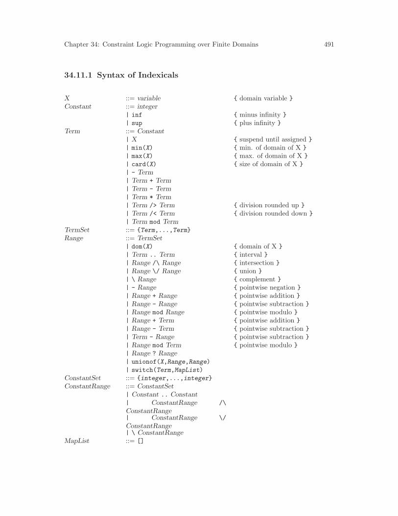
Chapter 34: Constraint Logic Programming over Finite Domains 491
34.11.1 Syntax of Indexicals
X ::= variable { domain variable }
Constant ::= integer| inf { minus infinity }
| sup { plus infinity }
Term ::= Constant| X { suspend until assigned }
| min(X) { min. of domain of X }
| max(X) { max. of domain of X }
| card(X) { size of domain of X }
| - Term| Term + Term| Term - Term| Term * Term| Term /> Term { division rounded up }
| Term /< Term { division rounded down }
| Term mod TermTermSet ::= {Term,...,Term}
Range ::= TermSet| dom(X) { domain of X }
| Term .. Term { interval }| Range /\ Range { intersection }
| Range \/ Range { union }
| \ Range { complement }| - Range { pointwise negation }
| Range + Range { pointwise addition }
| Range - Range { pointwise subtraction }
| Range mod Range { pointwise modulo }
| Range + Term { pointwise addition }
| Range - Term { pointwise subtraction }
| Term - Range { pointwise subtraction }
| Range mod Term { pointwise modulo }
| Range ? Range| unionof(X,Range,Range)
| switch(Term,MapList)
ConstantSet ::= {integer,...,integer}
ConstantRange ::= ConstantSet| Constant .. Constant| ConstantRange /\
ConstantRange| ConstantRange \/
ConstantRange| \ ConstantRange
MapList ::= []
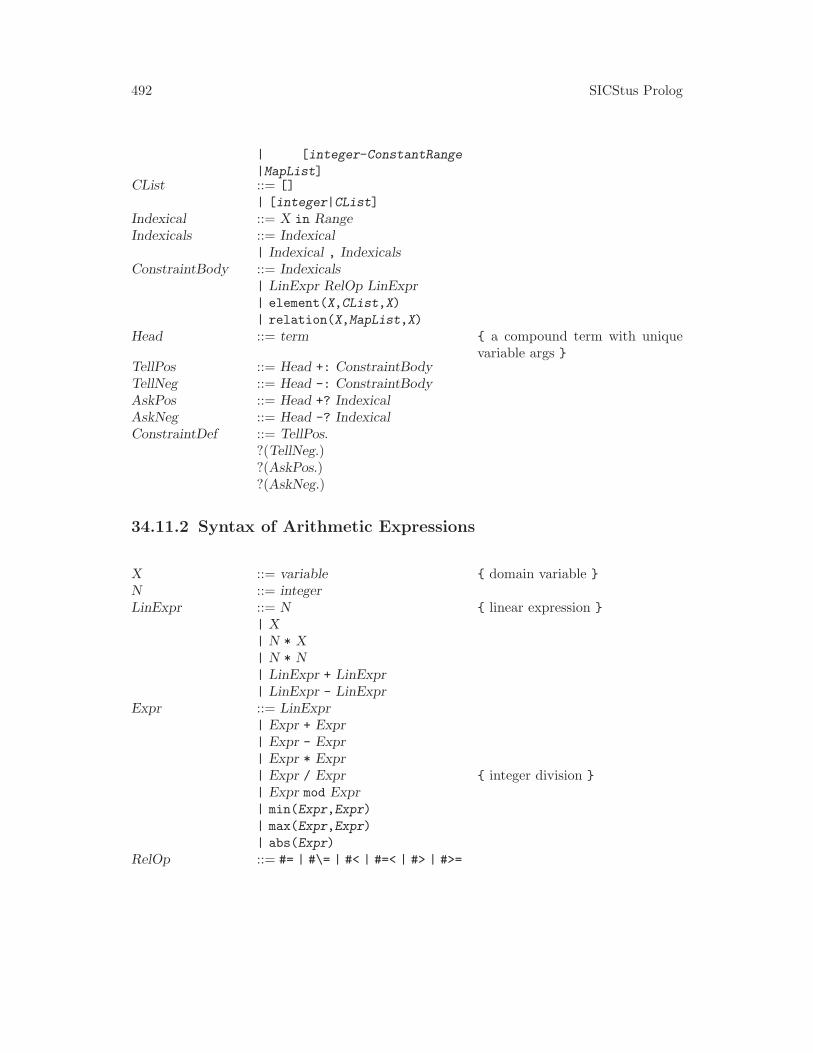
492 SICStus Prolog
| [integer-ConstantRange
|MapList]CList ::= []
| [integer|CList]
Indexical ::= X in RangeIndexicals ::= Indexical
| Indexical , IndexicalsConstraintBody ::= Indexicals
| LinExpr RelOp LinExpr| element(X,CList,X)
| relation(X,MapList,X)
Head ::= term { a compound term with uniquevariable args }
TellPos ::= Head +: ConstraintBodyTellNeg ::= Head -: ConstraintBodyAskPos ::= Head +? IndexicalAskNeg ::= Head -? IndexicalConstraintDef ::= TellPos.
?(TellNeg.)?(AskPos.)?(AskNeg.)
34.11.2 Syntax of Arithmetic Expressions
X ::= variable { domain variable }
N ::= integerLinExpr ::= N { linear expression }
| X| N * X| N * N| LinExpr + LinExpr| LinExpr - LinExpr
Expr ::= LinExpr| Expr + Expr| Expr - Expr| Expr * Expr| Expr / Expr { integer division }
| Expr mod Expr| min(Expr,Expr)
| max(Expr,Expr)
| abs(Expr)
RelOp ::= #= | #\= | #< | #=< | #> | #>=

Chapter 34: Constraint Logic Programming over Finite Domains 493
34.11.3 Operator Declarations
:- op(1200, xfx, [+:,-:,+?,-?]).
:- op(760, yfx, #<=>).
:- op(750, xfy, #=>).
:- op(750, yfx, #<=).
:- op(740, yfx, #\/).
:- op(730, yfx, #\).
:- op(720, yfx, #/\).
:- op(710, fy, #\).
:- op(700, xfx, [in,in_set]).
:- op(700, xfx, [#=,#\=,#<,#=<,#>,#>=]).
:- op(550, xfx, ..).
:- op(500, fy, \).
:- op(490, yfx, ?).
:- op(400, yfx, [/>,/<]).


![Constraint Logic Programming - MathUniPDfrossi/gulp.pdf · solvers added to a LP language becomes almost unlimited (e.g., [110]). 2.1 Finite Domains A popular class of constraints](https://img.dokumen.tips/doc/110x75/5f43502ab529c74c64766ec3/constraint-logic-programming-mathunipd-frossigulppdf-solvers-added-to-a-lp.jpg)


![arXiv:1502.04969v3 [math.NA] 10 Feb 2016 · 2018-05-02 · patch together several cubic domains to obtain this topology.) The operator is not elliptic, unless an additional constraint](https://img.dokumen.tips/doc/110x75/5fb9d80f0a4bc244cb63c731/arxiv150204969v3-mathna-10-feb-2016-2018-05-02-patch-together-several-cubic.jpg)