Embed Size (px)
Citation preview
University of Birmingham Research Archive
e-theses repository This unpublished thesis/dissertation is copyright of the author and/or third parties. The intellectual property rights of the author or third parties in respect of this work are as defined by The Copyright Designs and Patents Act 1988 or as modified by any successor legislation. Any use made of information contained in this thesis/dissertation must be in accordance with that legislation and must be properly acknowledged. Further distribution or reproduction in any format is prohibited without the permission of the copyright holder.
2nd of 5 files
Chapters 3 and 4
EFFECT OF STRESS ON INITIATION AND PROPAGATION OF LOCALIZED CORROSION IN
ALUMINIUM ALLOYS By
SUKANTA GHOSH
A thesis submitted to University of Birmingham
for the degree of DOCTOR OF PHILOSOPHY
Metallurgy and Materials School of Engineering
University of Birmingham
November 2007
Chapter 3. Experimental Procedure
108
3 EXPERIMENTAL PROCEDURE
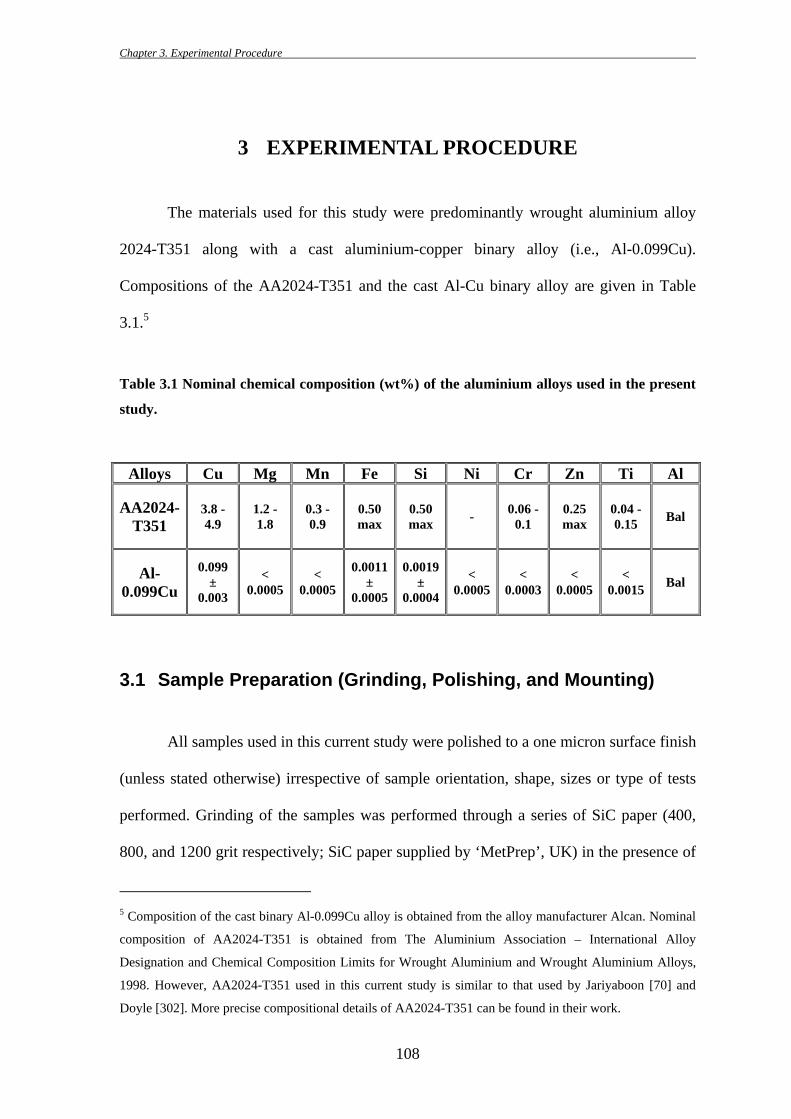
The materials used for this study were predominantly wrought aluminium alloy
2024-T351 along with a cast aluminium-copper binary alloy (i.e., Al-0.099Cu).
Compositions of the AA2024-T351 and the cast Al-Cu binary alloy are given in Table
3.1.5
Table 3.1 Nominal chemical composition (wt%) of the aluminium alloys used in the present
study.
Alloys Cu Mg Mn Fe Si Ni Cr Zn Ti Al
AA2024-T351
3.8 -4.9
1.2 -1.8
0.3 - 0.9
0.50 max
0.50 max - 0.06 -
0.1 0.25 max
0.04 - 0.15 Bal
Al-0.099Cu
0.099 ±
0.003
< 0.0005
< 0.0005
0.0011 ±
0.0005
0.0019 ±
0.0004
< 0.0005
< 0.0003
< 0.0005
< 0.0015 Bal
3.1 Sample Preparation (Grinding, Polishing, and Mounting)
All samples used in this current study were polished to a one micron surface finish
(unless stated otherwise) irrespective of sample orientation, shape, sizes or type of tests
performed. Grinding of the samples was performed through a series of SiC paper (400,
800, and 1200 grit respectively; SiC paper supplied by ‘MetPrep’, UK) in the presence of
5 Composition of the cast binary Al-0.099Cu alloy is obtained from the alloy manufacturer Alcan. Nominal
composition of AA2024-T351 is obtained from The Aluminium Association – International Alloy
Designation and Chemical Composition Limits for Wrought Aluminium and Wrought Aluminium Alloys,
1998. However, AA2024-T351 used in this current study is similar to that used by Jariyaboon [70] and
Doyle [302]. More precise compositional details of AA2024-T351 can be found in their work.
Chapter 3. Experimental Procedure
109
ethanol on the grinding machine. Contact of water during grinding was avoided as water
can attack the active ‘S’ phases present in the AA2024-T351 microstructure. Polishing of
the 1200 grit-ground samples was performed in 6 μm, 3 μm and 1 μm diamond
suspension (i.e., Struers “DiaDuo”) on “Mol” and “Nap” polishing cloths (Struers)
respectively. Samples were degreased and cleaned ultrasonically in ethanol for 2-3
minutes between different steps of grinding and polishing. After the final polish to one
micron diamond paste and ultrasonically cleaning, the samples were dried using a
conventional air blower.
A few samples were also mounted in epoxy resin for large scale ‘in beaker’
electrochemical tests (see Chapter 4) in order to expose only one surface with controlled
dimension. An electrical connection was created at the back of the samples with soldered
copper wire prior to the mounting of the samples in the epoxy resin. Resin was added in
sufficient quantity so that the connection at the back of the sample was completely
covered. Met Prep Variset 20 resin was used on these occasions and cured at room
temperature for at least 2 hours before electrochemical testing.
3.2 Characterization Techniques (Microstructural and Others)
Several characterizations techniques were used in this current study in order to
have a better understanding of the corrosion process associated with different
microstructural features. In many cases analysis of different intermetallic particles (as
well as intermetallic particle free areas) in AA2024-T351 were performed before and
after the electrochemical tests to emphasize the local changes happening during the
exposure.
Chapter 3. Experimental Procedure
110
3.2.1 Metallographic Etching
Metallographic etching of the cast Al-0.099Cu binary alloy was performed using
an etchant made of 2% HF + 10 % HNO3 to reveal the cast microstructure of the alloy.
The etchant was gently rubbed on the one micron polished sample surface using a cotton
bud for approximately 30 seconds and then rinsed with de-ionised water. Whenever
required the procedure was repeated for shorter times in order to achieve a clearly visible
grain structure. Etching of AA2024-T351 was not performed in this current study but was
performed on the same material in other work [70, 302].
3.2.2 Optical Microscopy
Optical microscopy was performed with a Zeiss Axiolab direct microscope with
magnifications up to 400X. The optical microscope was equipped with a KS300 3.0
Imaging system (Imaging Associates, UK) for further image analysis. Corroded surfaces
were cleaned (i.e., ultrasonically in ethanol, de-ionised water and then dried) prior to the
optical micrography.
3.2.3 Scanning Electron Microscopy (SEM)
Electron microscopy was performed using JEOL 6060, 6300, 7000 FEG-SEM
(JEOL Instruments, Japan) and a Philips XL-30 (Philips Instruments, UK). The
microscopes were used in both secondary and backscattered mode with an accelerating
voltage of 15-20 kV and a working distance of 10mm. In most cases, the samples were
Chapter 3. Experimental Procedure
111
mounted on aluminium stubs with adhesive carbon tape and silver paint in order to obtain
good electrical contact between the samples and the sample holder. All electron
microscopes were equipped with an EDX detector for chemical compositional analysis.
Analysis of the EDX data was carried out using INCA software (Oxford Instruments,
UK). SEMs quipped with EDX were used to perform composition analysis of different
intermetallic particles (before and after the electrochemical tests) as well as to document
the surface morphology after electrochemical experiments. A Hitachi FEG-SEM (Model
S-4000) in conjunction with a 10 kN servo-electric loading stage was used for in situ
study of intermetallic particle/alloy matrix delamination as a function of applied stress
(see Chapter 6).
3.2.4 Atomic Force Microscopy
Atomic force microscopy (Q-Scope 350 AFM, supplied by Quesant Instrument
Corporation, US) in contact mode was used in this current study to characterize the
corrosion behaviour of individual intermetallic particles subjected to electrochemical
investigation using a micro-capillary electrochemical cell. Morphology of the
intermetallic particles and the surrounding matrix were investigated before and after the
corrosion (potentiodynamic, potentiostatic or free corrosion/open circuit potential) tests.
A maximum scan area of 80 µm × 80 µm and maximum depth of 5 µm was achieved
using this set up. A scan rate of 1 Hz was used for good quality images. Analysis of the
AFM data was performed using Q-AnalysisTM software. It was found that flatness of the
samples was very crucial to obtain good tomographic images of the intermetallic
particles. Throughout the AFM experiments, care was taken to ensure that the top surface
Chapter 3. Experimental Procedure
112
of the specimens remained flat using a leveller. AFM was predominantly used to study
the nature of grooving (depth and width of the grooves, discontinuous vs. continuous etc.)
around the intermetallic particles during the current study (see Chapter 5 and 6).
3.2.5 Line Profilometry
A Stylet Profilometer DekTak® 6M (from Vecco, US) was used to measure the
surface dissolution of AA2024-T351 samples during the surface treatment for ‘S’ phase
removal (see Chapter 4). Prior to surface treatment, one part of the sample’s surface (one
micron surface finish) was covered with ‘Stop-Off’ lacquer and rest left uncovered. The
whole sample was then subjected to surface treatment. After the surface treatment, the
‘Stop-Off’ lacquer was removed and line profilometric analysis was performed at the
junction between the surface-treated and untreated areas on the sample. Step heights
between these two areas gave an estimation of material dissolution during the surface
treatment. A stylet of 2.5 µm radius with a force of 3 mg was used during the
profilometric analysis. The length measured was 2000 µm for a total duration of 60 s.
3.2.6 Optical Profilometry
High resolution optical profilometry was carried out with an Altisurf 500 white
light profilometer (from Cotec, France) with a sensor having a dynamic range of 50 nm –
300 µm. This technology involves a white light source (quartz-halogen) that is focused
onto a sample through a lens that displays a high level of chromatic aberration. The
chromatic aberration is then used to precisely measure the position of a particular surface
Chapter 3. Experimental Procedure
113
element with respect to a reference point. This non-contact technique can give accurate
height information (to a resolution of 5 nanometres) about the 3D surface structure of any
material over an area of up to 10 square centimetres. Results were evaluated using
Altimap software (see Chapter 5).
3.2.7 Surface Mapping using Microhardness Markers
A microhardness tester was used as a surface mapping tool in this current study
rather than measuring the hardness of the material (see Chapter 5 and 6). A Mitutoyo
MVK-H1 hardness testing machine (Mitutoyo Ltd, UK) with a load of 100g was used to
create the indentation marks. The sample surface (polished to one micron) was marked
with a grid of indentations as shown in Figure 3.1. Indentations with a diagonal length of
~ 34 µm (at 100g load) were made at a distance of one mm from each other. An
indentation was also created adjacent to the grid for reference. The samples with
indentation marks on their surface were subjected to SEM analysis prior to the
electrochemical tests. Different types of intermetallic particles (as well as areas without
any intermetallic particles) were identified/analysed using EDX and their co-ordinates
were noted with respect to their nearest indentation mark.

Chapter 3. Experimental Procedure
114
Figure 3.1 Schematic of AA2024-T351 surface mapped with microhardness indentations.
Indentations are made at a distance of one mm from each other. One extra indentation is
made adjacent to the grid as the reference point. These indentations have a diagonal length
of about 34 µm when 100 g load is maintained. L = Longitudinal direction, T = Transverse
direction.
After the SEM analysis, the surface mapped samples were lightly polished with
one micron diamond paste to remove any possible carbon deposition and contamination
on the surface. Relatively deep indentations with 100g load ensured the presence of marks
even after light repolishing. This process provided the easier way of particle identification
before and after micro-capillary electrochemical cell test. It should be noted that though
Fe-Mn particles were visible via optical microscopy, smaller S phase particles were
difficult to image using the lower magnification optics attached with the micro-capillary
electrochemical cell test set up. After the micro-capillary electrochemical tests (with an
exposed area of 40 µm diameter), the exposed intermetallic particles (or the particle free
matrix) were again subjected to SEM and EDX analysis based on their previously
determined co-ordinate position with respect to the nearest microhardness markers.
1 mm
1 mm
T
L
1 mm
1 mm
1 mm
1 mm
T
L
Chapter 3. Experimental Procedure
115
3.3 Surface Treatment
Prior to the surface treatment, all samples were finally polished to one micron
surface finish as described in Section 3.1. Polished samples were then degreased with
methanol in an ultrasonic bath for 2 minutes. For the standard surface treatment, the
samples were etched in 3g/l sodium hydroxide (NaOH) for 10 minutes, rinsed under
running tap water for 2 minutes, desmutted for 30s in nitric acid [i.e., 1:2 (vol) of water :
70% nitric acid] and finally rinsed for 5 minutes under running tap water. In some cases
(whenever necessary), 10 mM CeCl3 salt was added in the nitric acid while desmutting.
3.4 Electrochemical Tests with ‘Large’ Exposure Area (‘In Beaker Cell’)
3.4.1 The Samples
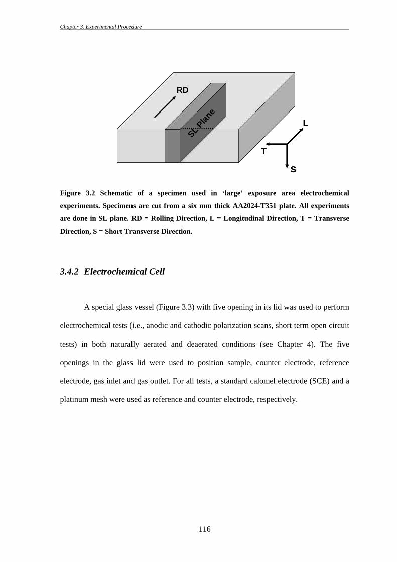
Samples of 35 mm length and 3 mm width were cut from a six mm thick AA2024-
T351 plate as shown in Figure 3.2. All experiments were performed on the SL plane of
the samples as indicated in the figure. One micron surface finish was used for all
experiments unless stated otherwise. Exposed areas of the samples were controlled by
lacquering (with ‘Stopping Off’ lacquer) the surface. Exposed areas were varied from 1.2
cm2 (24 mm × 5mm) to as small as 0.01 cm2 (1 mm × 1 mm) depending on the
experiments performed (see Chapter 4). A few samples were mounted in epoxy resin by
the process described in Section 3.1. Areas between the sample edge and the epoxy resin
were lacquered to avoid any crevice corrosion. In all cases lacquer was applied in several
layers and dried completely prior to any electrochemical tests.
Chapter 3. Experimental Procedure
116
Figure 3.2 Schematic of a specimen used in ‘large’ exposure area electrochemical
experiments. Specimens are cut from a six mm thick AA2024-T351 plate. All experiments
are done in SL plane. RD = Rolling Direction, L = Longitudinal Direction, T = Transverse
Direction, S = Short Transverse Direction.
3.4.2 Electrochemical Cell
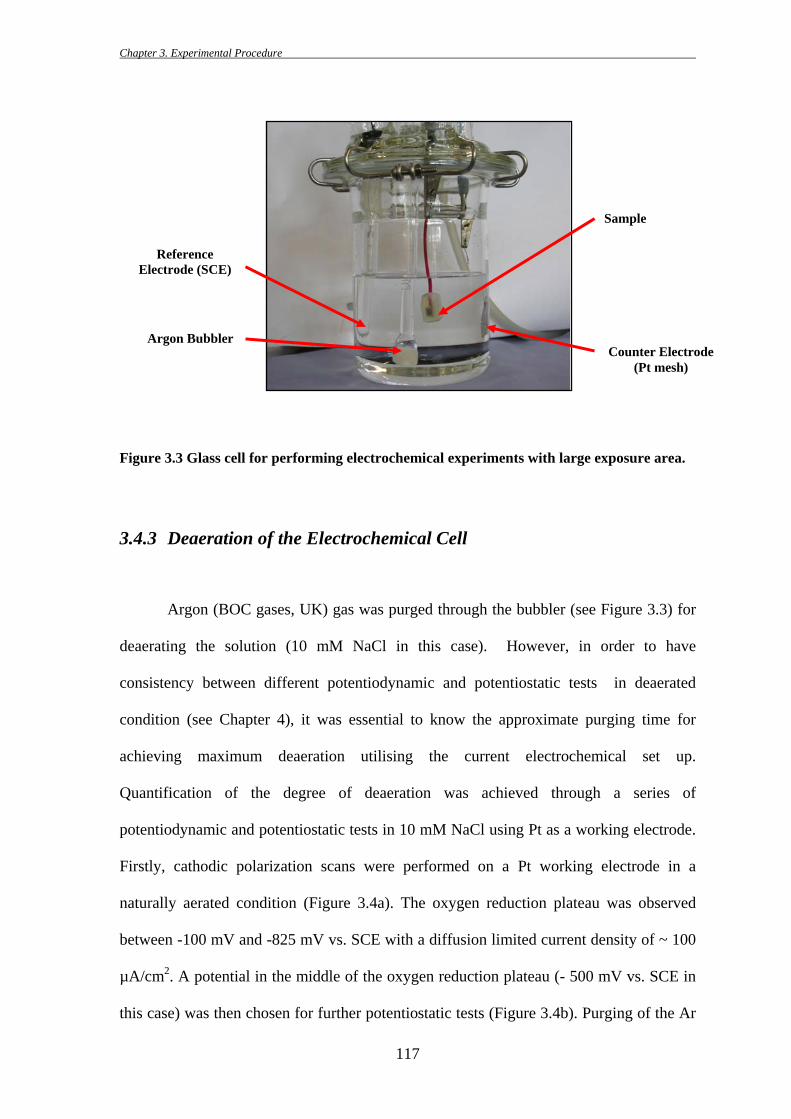
A special glass vessel (Figure 3.3) with five opening in its lid was used to perform
electrochemical tests (i.e., anodic and cathodic polarization scans, short term open circuit
tests) in both naturally aerated and deaerated conditions (see Chapter 4). The five
openings in the glass lid were used to position sample, counter electrode, reference
electrode, gas inlet and gas outlet. For all tests, a standard calomel electrode (SCE) and a
platinum mesh were used as reference and counter electrode, respectively.
L
S
T
RD
SL Plan
e
L
S
T
RD
SL Plan
e
Chapter 3. Experimental Procedure
117
Figure 3.3 Glass cell for performing electrochemical experiments with large exposure area.
3.4.3 Deaeration of the Electrochemical Cell
Argon (BOC gases, UK) gas was purged through the bubbler (see Figure 3.3) for
deaerating the solution (10 mM NaCl in this case). However, in order to have
consistency between different potentiodynamic and potentiostatic tests in deaerated
condition (see Chapter 4), it was essential to know the approximate purging time for
achieving maximum deaeration utilising the current electrochemical set up.
Quantification of the degree of deaeration was achieved through a series of
potentiodynamic and potentiostatic tests in 10 mM NaCl using Pt as a working electrode.
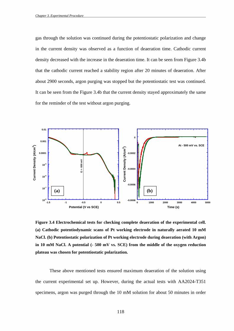
Firstly, cathodic polarization scans were performed on a Pt working electrode in a
naturally aerated condition (Figure 3.4a). The oxygen reduction plateau was observed
between -100 mV and -825 mV vs. SCE with a diffusion limited current density of ~ 100
µA/cm2. A potential in the middle of the oxygen reduction plateau (- 500 mV vs. SCE in
this case) was then chosen for further potentiostatic tests (Figure 3.4b). Purging of the Ar
Sample
Counter Electrode (Pt mesh)
Reference Electrode (SCE)
Argon Bubbler
Chapter 3. Experimental Procedure
118
gas through the solution was continued during the potentiostatic polarization and change
in the current density was observed as a function of deaeration time. Cathodic current
density decreased with the increase in the deaeration time. It can be seen from Figure 3.4b
that the cathodic current reached a stability region after 20 minutes of deaeration. After
about 2900 seconds, argon purging was stopped but the potentiostatic test was continued.
It can be seen from the Figure 3.4b that the current density stayed approximately the same
for the reminder of the test without argon purging.
Figure 3.4 Electrochemical tests for checking complete deaeration of the experimental cell.
(a) Cathodic potentiodynamic scans of Pt working electrode in naturally aerated 10 mM
NaCl. (b) Potentiostatic polarization of Pt working electrode during deaeration (with Argon)
in 10 mM NaCl. A potential (- 500 mV vs. SCE) from the middle of the oxygen reduction
plateau was chosen for potentiostatic polarization.
These above mentioned tests ensured maximum deaeration of the solution using
the current experimental set up. However, during the actual tests with AA2024-T351
specimens, argon was purged through the 10 mM solution for about 50 minutes in order
10-8
10-7
10-6
10-5
0.0001
0.001
0.01
-1.5 -1 -0.5 0 0.5
Cur
rent
Den
sity
(A/c
m2 )
Potential (V vs SCE)
E =
-500
mV
-0.0008
-0.0006
-0.0004
-0.0002
0
0 1000 2000 3000 4000 5000
Cur
rent
Den
sity
(A/c
m2 )
Time (s)
At - 500 mV vs. SCE
(a) (b)

Chapter 3. Experimental Procedure
119
to minimise the presence of any residual oxygen. AA2024-T351 specimens were kept
above the solution inside the closed cell during deaeration and were pushed into the
solution before beginning of the electrochemical tests at the end of argon purging. At the
end of 50 minutes of purging, the argon bubbler was lifted just above the solution level
and kept purging with a very slow flow rate. This ensured the presence of argon blanket
inside the cell during the electrochemical tests.
3.4.4 Potentiodynamic Polarization Experiments
Potentiodynamic polarization experiments were carried out utilising a Solartron
1280 or 1285 potentiostat controlled via computer through CorrWare V2.0 software.
3.4.4.1 Anodic Polarization Scans
Anodic polarization scans were performed on one micron surface finished
AA2024-T351 samples in both surface treated and untreated conditions at room
temperature. 10 mM NaCl solution in naturally aerated and deaerated conditions was used
to perform the test. Scans were started at 20 mV negative to the open circuit potential and
continued with a scan rate of 1 mV/s to the anodic (i.e., positive) direction. Prior to the
start of the experiment, samples were held at open circuit for one to five minutes
depending on the stability of the potentials.
Chapter 3. Experimental Procedure
120
3.4.4.2 Cathodic Polarization Scans
The cathodic polarization scans were performed in naturally aerated 10 mM NaCl
as well as in different buffer solutions at room temperature (see Chapter 4). Scans were
started at 20 mV positive to the open circuit and continued with a scan rate of 1 mV/s to
the cathodic (i.e., negative) direction until -1.8 V vs. the reference. Buffer solutions [171,
303] used in the experiments were:
i) 0.1 M H3BO3 adjusted to pH 7 by the addition of 1 M NaOH
ii) 0.1 M Na2HPO4 adjusted to pH 7 by 4 M H3PO4
3.4.5 Potentiostatic Polarization Experiments
Samples were polished to one micron and surface treated as required. In a few
cases 800 grit surface finish were also used as rough surface were thought to enhance the
possibility of detecting metastable activities by increasing its frequency of occurrence.
However, at any given potential, comparison of the corrosion properties between the
surface treated and untreated samples were always made under similar surface finishing.
Different sample areas (i.e., from 1.2 cm2 to as small as 0.01 cm2) were used to capture
the metastable pitting transients. These experiments were also carried out with Solartron
1280 or 1285 potentiostat operating with CorrWare V2.0 software.
All the tests were performed in 10 mM NaCl solution either in naturally aerated or
deaerated condition at room temperature (see Chapter 4). Based on the anodic
polarization scans different potentials were chosen for further potentiostatic polarizations.
Potentials were varied from -575 mV vs. SCE (in the passive region) to -500 mV vs. SCE
Chapter 3. Experimental Procedure
121
(close to pitting potential) to find transients correspond to metastable pitting. The data
was collected at a frequency of 10 Hz (10 points/s). Higher the frequency of data
collection ensured a greater chance to capture each transients and obtaining a smooth
curve. Samples were inspected in optical as well as under SEM to identify and quantify in
size the metastable and stable pitting associated with the electrochemical data.
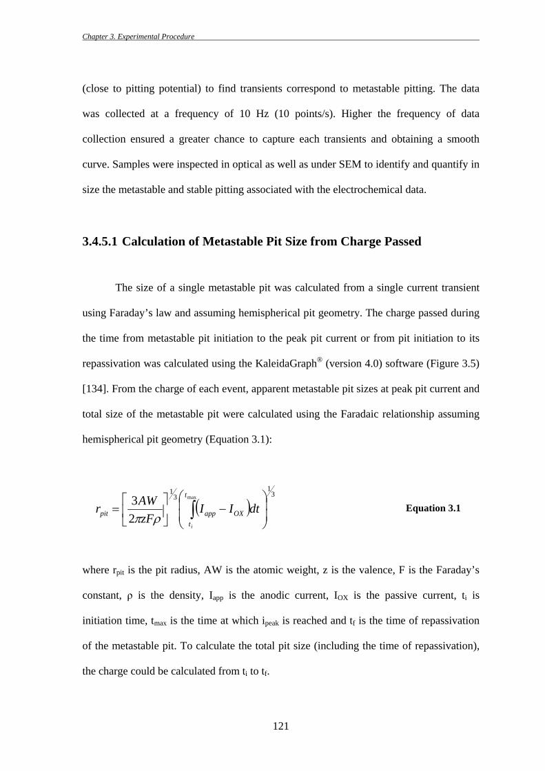
3.4.5.1 Calculation of Metastable Pit Size from Charge Passed
The size of a single metastable pit was calculated from a single current transient
using Faraday’s law and assuming hemispherical pit geometry. The charge passed during
the time from metastable pit initiation to the peak pit current or from pit initiation to its
repassivation was calculated using the KaleidaGraph® (version 4.0) software (Figure 3.5)
[134]. From the charge of each event, apparent metastable pit sizes at peak pit current and
total size of the metastable pit were calculated using the Faradaic relationship assuming
hemispherical pit geometry (Equation 3.1):
( )3
13
1max
23
⎟⎟⎠
⎞⎜⎜⎝
⎛−⎥
⎦
⎤⎢⎣
⎡= ∫
t
tOXapppit
i
dtIIzFAWr
ρπ Equation 3.1
where rpit is the pit radius, AW is the atomic weight, z is the valence, F is the Faraday’s
constant, ρ is the density, Iapp is the anodic current, IOX is the passive current, ti is
initiation time, tmax is the time at which ipeak is reached and tf is the time of repassivation
of the metastable pit. To calculate the total pit size (including the time of repassivation),
the charge could be calculated from ti to tf.
Chapter 3. Experimental Procedure
122
Figure 3.5 Schematic showing the limits of numerical integration of a metastable pitting
event.
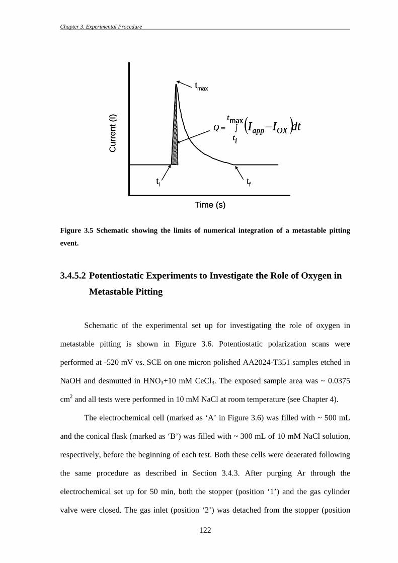
3.4.5.2 Potentiostatic Experiments to Investigate the Role of Oxygen in
Metastable Pitting
Schematic of the experimental set up for investigating the role of oxygen in
metastable pitting is shown in Figure 3.6. Potentiostatic polarization scans were
performed at -520 mV vs. SCE on one micron polished AA2024-T351 samples etched in
NaOH and desmutted in HNO3+10 mM CeCl3. The exposed sample area was ~ 0.0375
cm2 and all tests were performed in 10 mM NaCl at room temperature (see Chapter 4).
The electrochemical cell (marked as ‘A’ in Figure 3.6) was filled with ~ 500 mL
and the conical flask (marked as ‘B’) was filled with ~ 300 mL of 10 mM NaCl solution,
respectively, before the beginning of each test. Both these cells were deaerated following
the same procedure as described in Section 3.4.3. After purging Ar through the
electrochemical set up for 50 min, both the stopper (position ‘1’) and the gas cylinder
valve were closed. The gas inlet (position ‘2’) was detached from the stopper (position
Time (s)
Cur
rent
(I)
( )dtIIt
itOXappQ ∫= −max
ti
tmax
tf
Time (s)
Cur
rent
(I)
( )dtIIt
itOXappQ ∫= −max
ti
tmax
tf
Chapter 3. Experimental Procedure
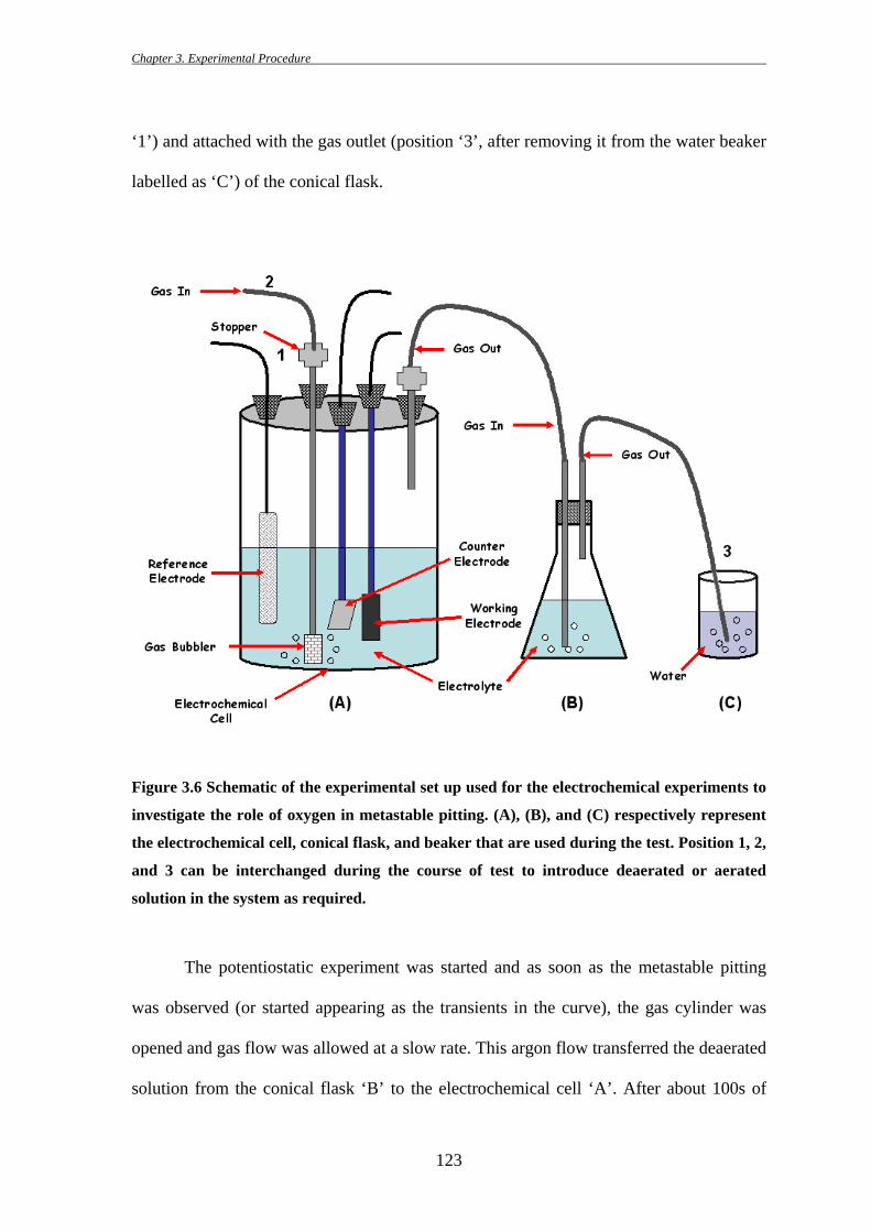
123
‘1’) and attached with the gas outlet (position ‘3’, after removing it from the water beaker
labelled as ‘C’) of the conical flask.
Figure 3.6 Schematic of the experimental set up used for the electrochemical experiments to
investigate the role of oxygen in metastable pitting. (A), (B), and (C) respectively represent
the electrochemical cell, conical flask, and beaker that are used during the test. Position 1, 2,
and 3 can be interchanged during the course of test to introduce deaerated or aerated
solution in the system as required.
The potentiostatic experiment was started and as soon as the metastable pitting
was observed (or started appearing as the transients in the curve), the gas cylinder was
opened and gas flow was allowed at a slow rate. This argon flow transferred the deaerated
solution from the conical flask ‘B’ to the electrochemical cell ‘A’. After about 100s of
Chapter 3. Experimental Procedure
124
potentiostatic hold, ~ 100 mL of deaerated solution was transferred to the electrochemical
cell ‘A’. Aerated solution (prepared in a separate glass vessel by passing air through the
solution for 40 minutes) was added in the electrochemical cell with a syringe through the
port used for the gas bubbler. Two batches of aerated solution were added at different
time intervals during the experiment with a quantity of 100 mL and 150 mL, respectively.
Both deaerated and aerated solution during the experiment was introduced in the system
with minimum of agitation.
3.4.6 Open Circuit Potential (OCP) Measurements
Open circuit potential (also referred as corrosion potential) tests of one micron
polished AA2024-T351 samples were performed in naturally aerated 10 mM NaCl in
both as-received and surface treated conditions at room temperature. Open circuit
potentials of these samples were measured either for a short time period (i.e., 15-30
minutes) or over a longer period (i.e., 3-4 days).
Solartron potentiostats (1280 or 1285) were used to collect the open circuit
potentials of the samples during the short duration exposure (i.e., 30 mins) in the beaker
cell (as shown in Figure 3.3). Epoxy resin mounted samples were used for long term open
circuit tests which were performed for 3-4 days by immersing the samples in
conventional beakers containing ~ 500 ml of naturally aerated 10 mM NaCl solution.
These beakers were immersed in a thermal bath maintained at 25˚C in order to control the
thermal fluctuations during the day-night continuous exposure. Corrosion potentials
(OCP) of these samples were monitored using a Keithley data logger Multimeter (Model
2000, Keithley Instruments, UK) with up to 10 channels being recorded simultaneously.
Chapter 3. Experimental Procedure
125
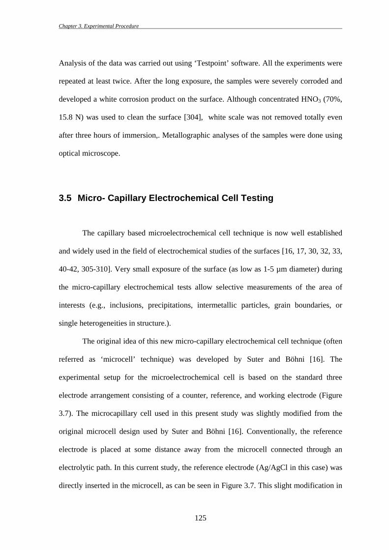
Analysis of the data was carried out using ‘Testpoint’ software. All the experiments were
repeated at least twice. After the long exposure, the samples were severely corroded and
developed a white corrosion product on the surface. Although concentrated HNO3 (70%,
15.8 N) was used to clean the surface [304], white scale was not removed totally even
after three hours of immersion,. Metallographic analyses of the samples were done using
optical microscope.
3.5 Micro- Capillary Electrochemical Cell Testing
The capillary based microelectrochemical cell technique is now well established
and widely used in the field of electrochemical studies of the surfaces [16, 17, 30, 32, 33,
40-42, 305-310]. Very small exposure of the surface (as low as 1-5 µm diameter) during
the micro-capillary electrochemical tests allow selective measurements of the area of
interests (e.g., inclusions, precipitations, intermetallic particles, grain boundaries, or
single heterogeneities in structure.).
The original idea of this new micro-capillary electrochemical cell technique (often
referred as ‘microcell’ technique) was developed by Suter and Böhni [16]. The
experimental setup for the microelectrochemical cell is based on the standard three
electrode arrangement consisting of a counter, reference, and working electrode (Figure
3.7). The microcapillary cell used in this present study was slightly modified from the
original microcell design used by Suter and Böhni [16]. Conventionally, the reference
electrode is placed at some distance away from the microcell connected through an
electrolytic path. In this current study, the reference electrode (Ag/AgCl in this case) was
directly inserted in the microcell, as can be seen in Figure 3.7. This slight modification in
Chapter 3. Experimental Procedure
126
the microcell design allowed experiments to be performed at lower concentration (0.1 M
NaCl) compared to the conventional microcell setup (0.5 M NaCl was the lowest
concentration possible in the conventional microcell setup possibly due to the IR drop
related issues).
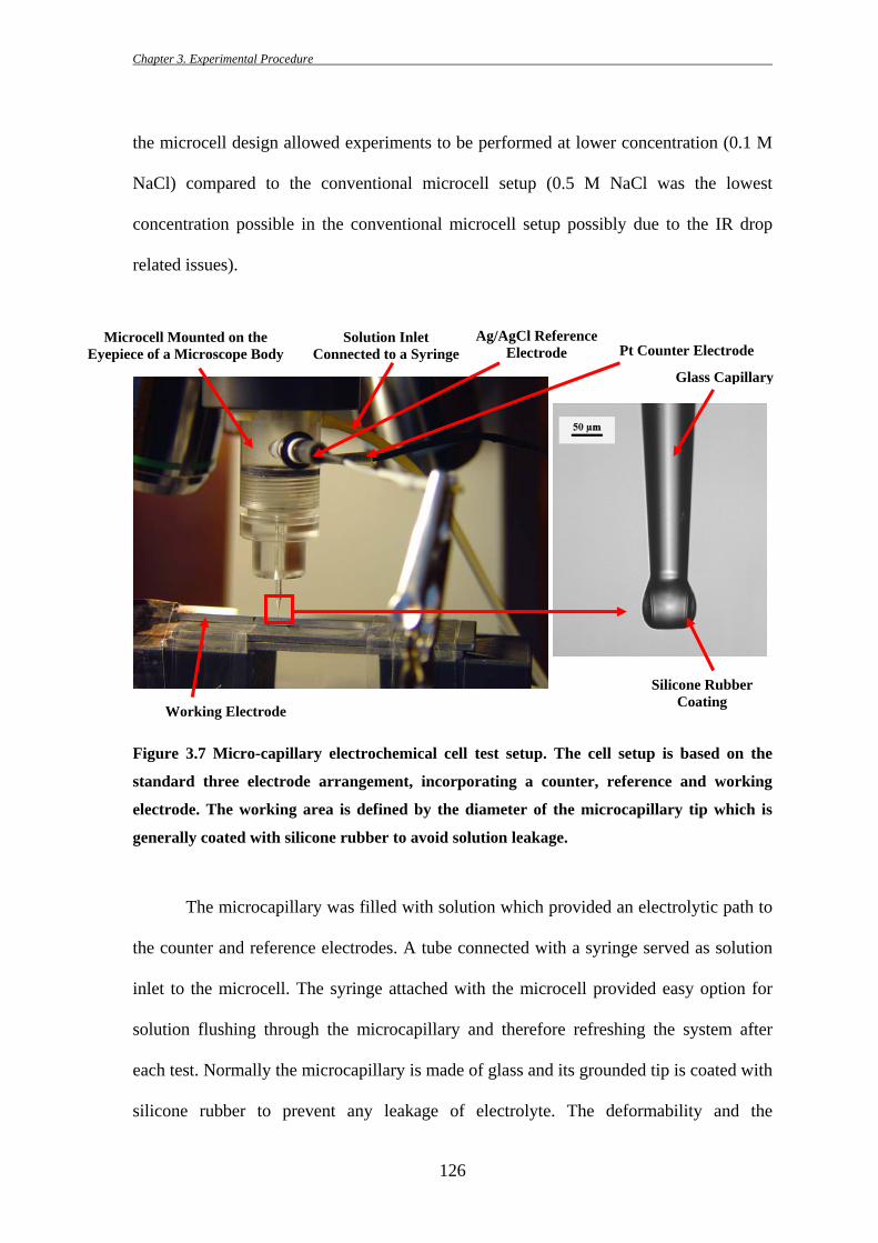
Figure 3.7 Micro-capillary electrochemical cell test setup. The cell setup is based on the
standard three electrode arrangement, incorporating a counter, reference and working
electrode. The working area is defined by the diameter of the microcapillary tip which is
generally coated with silicone rubber to avoid solution leakage.
The microcapillary was filled with solution which provided an electrolytic path to
the counter and reference electrodes. A tube connected with a syringe served as solution
inlet to the microcell. The syringe attached with the microcell provided easy option for
solution flushing through the microcapillary and therefore refreshing the system after
each test. Normally the microcapillary is made of glass and its grounded tip is coated with
silicone rubber to prevent any leakage of electrolyte. The deformability and the
Ag/AgCl Reference Electrode Pt Counter Electrode
Solution Inlet Connected to a Syringe
Microcell Mounted on the Eyepiece of a Microscope Body
Working Electrode
Glass Capillary
Silicone Rubber Coating
Chapter 3. Experimental Procedure
127
hydrophobic behaviour of the silicone rubber provides major advantages during
electrochemical measurement [17]. Excellent deformability of the silicone rubber permits
testing on a rough surface and the hydrophobic nature of silicone prevents formation of
crevices due to solution leakage under the seal.
Throughout this current micro-capillary electrochemical study (see Chapter 5 and
6), capillary tip diameter of was maintained at 40 µm (i.e., equivalent exposure area of 40
µm diameter). These microcapillaries were prepared by heating and pulling a borosilicate
glass capillary (Harvard Apparatus, 2.0 mm outer diameter and 1.16 inner diameter) using
a capillary puller (Narishige) once the melting temperature of the borosilicate glass was
reached. The pulled capillaries were then ground in 4000 grit SiC paper in the presence of
a lubricant (glycerine in this case) till the desired capillary diameter was reached.
Polished glass capillaries were then cleaned with ethanol, dried and coated with silicone
rubber (RS 555-588 Silicone Rubber Compound, RS Components, Northants, UK). A
stream of ethanol was passed through the microcapillary in order to flush out the silicone
inside the capillary without destroying the fine tip and silicone rubber skirt. A relatively
thick layer of silicone (normally the thickness of the silicone layer at the capillary tip was
equivalent to one-fifth of the capillary tip diameter) was applied to the capillary tip by
repeating this process several times. As the silicone cured very slowly, an interval of
about 30 min was maintained between two consecutive coatings to ensure hardening of
each layer. Microcapillaries coated with silicone were stored overnight prior to their use
in the microcell.
The fully assembled micro-capillary electrochemical cell setup along with
reference and counter electrode was then fixed at the revolving nosepiece on an optical
microscope, replacing an objective (Figure 3.7). The specimen was mounted on the
microscope stage. This arrangement enabled the search for a microstructural site utilising
Chapter 3. Experimental Procedure
128
different magnifications before switching to the microcapillary. It also allowed precise
positioning of the capillary on the area of interest. The microscope was attached with a
camera which allowed imaging of the surface under investigation before and after the
tests. The entire micro-capillary electrochemical cell setup was placed in a Faraday cage
to avoid any noise disturbance from adjacent equipment. Detailed discussion about the
micro-capillary electrochemical cell technique including capillary preparation can be
found elsewhere [17].
The micro-capillary electrochemical setup used in this study was connected to a
low noise CH potentiostat (CH Instruments, Model CHI600B) or with a modified high-
resolution potentiostat with a current detection limit of 20 fA (Jaissle Electronik GmbH,
Waiblingen, Germany 1002T-NC-3).6 Specimens used in this study were mechanically
ground by SiC papers (from 400 to 1200 grit) and polished with several grades of
diamond suspensions (from 6 µm to 1 µm). During grinding, sample contact with water
was avoided by using ethanol as a lubricant (as water can partially attack the S phases
which were later electrochemically tested). Detailed description of grinding and polishing
has been given earlier. Samples were cleaned ultrasonically in ethanol for 2-3 minutes
between different steps of grinding and polishing. After the final polish to one micron
diamond paste and ultrasonically cleaning, the samples were dried using a conventional
air blower.
It was found that the time between the final polishing and performing the micro-
capillary electrochemical tests were crucial. So, after final polishing, samples were kept
1.5 – 2 hours in air before starting the tests. All tests on a single specimen were
6 Microcapillary electrochemical cell experiments with the ‘Jaissle’ potentiostat were performed in the
LRRS, Université de Bourgogne, Dijon, France as a part of an International collaboration funded by the
Royal Society, UK.
Chapter 3. Experimental Procedure
129
performed on the same day as it was found that leaving the sample overnight sometime
gave problem in running the tests.7 Naturally aerated NaCl solution of 0.1 M and 0.5 M
concentration was used in the micro-capillary electrochemical tests. All experiments in
the microcapillary electrochemical cell were carried out at room temperature. All
potentiodynamic scans were started at a specified potential (-1000 mV, -800 mV, -700
mV vs. Ag/AgCl etc.) without any delay at open circuit potential. The scan rate (or sweep
rate) for all potentiodynamic scans was set at 1 mV/s. The controlling computer programs
were set in such a way that, the potentiodynamic experiments were terminated once the
current reached a value of 10 nA.
In many cases, microhardness markers were used to identify specific intermetallic
particle location. These markers helped in finding the particles on the specimen surface
and made capillary positioning easier. The compositions of those intermetallic particles
were confirmed using EDS analysis. After SEM and EDS investigations the surface
mapped specimens (i.e., array of microhardness markers 1 mm apart from each other on
the specimen surface along with identified areas of interest with respect to the grid
markers – see Section 3.2.7) were lightly polished in one micron diamond paste prior to
the micro-capillary electrochemical tests.
7 Samples stored overnight sometimes showed problem in creating proper contact (which was necessary to
run the electrochemical test) between the capillary and the specimen. Sometimes the potentiodynamic scans
showed almost a constant cathodic current and sudden breakdown without showing any definite open
circuit potential and passive region.
Chapter 3. Experimental Procedure
130
3.6 Mechanical Tests Associated with Stress Assisted Localized Corrosion Studies
3.6.1 Mechanical Testing of AA2024-T351
Tensile samples were made from the mid-plane of a rolled AA2024-T351 plate of
6 mm thickness. The rolled plate was milled on both faces to make the samples
approximately 3 mm thick. Samples were cut in such a way that the applied stress was
parallel to the rolling direction of the plate. The gauge length of the samples was fixed to
40 mm whereas the width of the specimen was 15 mm. Samples were ground to 1200 grit
sand paper to ensure a smooth surface finish. A Zwick 1484 twin screw re-circulating ball
universal tensile tester with a 200 kN (dynamic ± 200 kN) load cell mounted on an X-
head was used for the tensile tests. As the specimens were flat, 100 kN Instron strip grips
mounted axially in the load train were used during the course of experiment. The cross
head speed of the tensile machine was maintained at 1 mm/min and this speed yielded a
strain rate of 4.17 × 10⁻⁴ s-1. Each experiment was carried out until the specimen fractured
(see Chapter 6). A PC based data acquisition system was used to control the machine
operation and data recording. Raw data was taken out, plotted, and analysed using
‘KaleidaGraph’ software. Elastic modulus (E), proof stress at 0.2% strain (referred as
Yield Stress in this current study), stress at maximum load (ultimate tensile strength) and
strain at fracture was calculated for each specimen of AA2024-T351. Tensile tests were
also performed on a sensitized temper of AA2024 (i.e., heat treated at 250˚C for 2 h,
followed by water quenching) in similar manner.8
8 In this case, stress was applied perpendicular to the rolling direction.
Chapter 3. Experimental Procedure
131
3.6.2 Four Point Bend Stressing Set Up for In Situ SEM Studies
Samples were prepared from the middle section of a 6 mm thick plate of AA2024-
T351. Top and bottom faces of the plate were milled first and then samples with 34.5 mm
length, 10 mm width and 3 mm thickness were manufactured from it using a diamond
blade cutter (Figure 3.8). Samples were cut in different orientations such that stress could
be applied parallel and perpendicular to the stressing direction. Samples were then
polished to 1 micron diamond surface finish and finally polished with colloidal silica.
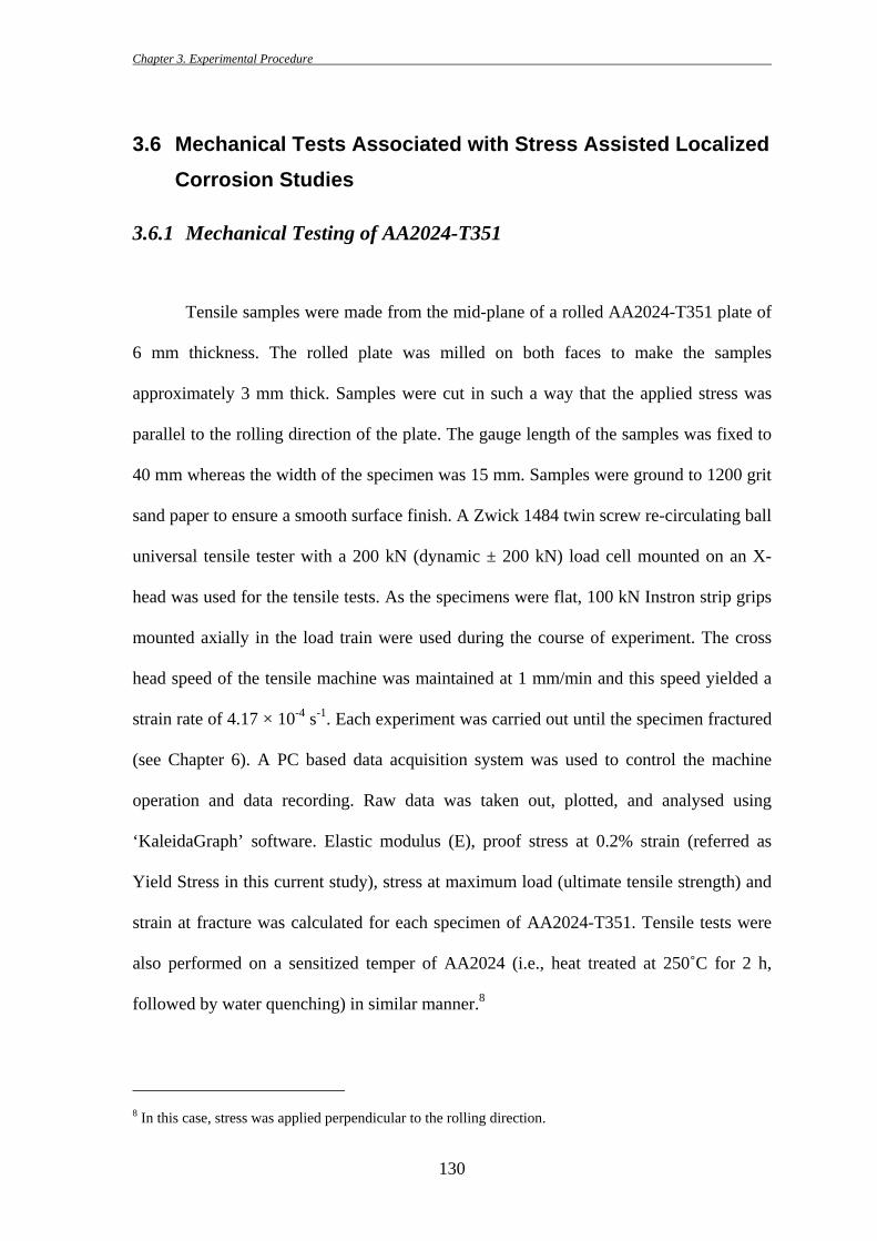
A four point bending set up was used (Figure 3.9) in the stressing stage for in situ9
study using a high resolution Hitachi FEG-SEM (Model S-4000). The applied load using
this four-point bend set up was calculated using Equation 3.2.
aWT
P3
2max
maxσ
= Equation 3.2
where, P = Applied load, σ = Stress, W = Width of the specimen, T = Thickness of the
specimen, and a = 9 mm in this case.
It was very difficult to control the effective load using the load cell attached with
the four-point bend test set up in the servo electric stressing stage. It has also to be noted
that the load cell on the servo electric stressing stage is calibrated for tensile-tensile
loading and not for four-point bend set up. Hence, a strain gauge was used to calculate the
applied stress (as a percentage of yield stress) more precisely. Tokyo Sokki Kenkyuyo
FLK-1-23 strain gauges (3 mm long and 1 mm wide) were mounted on the top surface of
9 In these in situ experiments, stress was applied on the sample during the SEM analysis (i.e., when the
sample mounted on the stressing stage was actually inside the vacuum chamber of the microscope).
Chapter 3. Experimental Procedure
132
the sample using superglue (Figure 3.8). After firmly fixing the strain gauge to the
surface, it was coated with silicone rubber to prevent the superglue from dissolving
during the final stage of cleaning with ethanol.
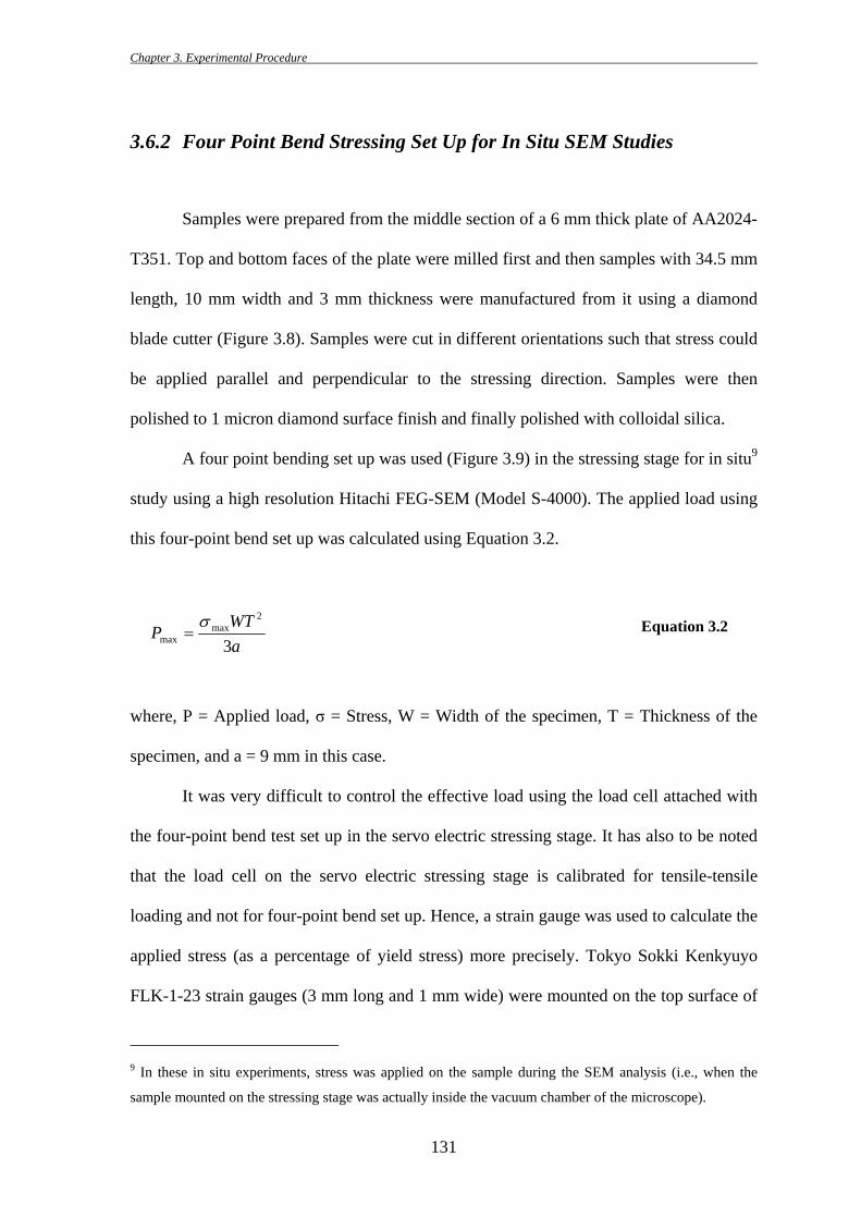
Figure 3.8 Orientations of the specimen prepared from the AA2024-T351 rolled plate. RD =
Rolling Direction, L = Longitudinal Direction, T = Transverse Direction, S = Short
Transverse Direction. Load is applied parallel or perpendicular to the rolling direction.
Observations are made on the L-T plane of the sample. Strain gauge is fixed on the top of
the surface.
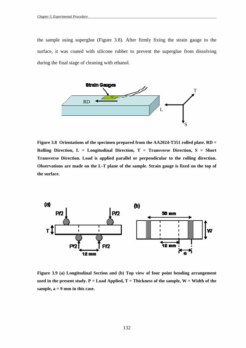
Figure 3.9 (a) Longitudinal Section and (b) Top view of four point bending arrangement
used in the present study. P = Load Applied, T = Thickness of the sample, W = Width of the
sample, a = 9 mm in this case.
T
L
S
RD
Chapter 3. Experimental Procedure
133
0
500
1000
1500
2000
2500
0 2000 4000 6000 8000 1 104 1.2 104 1.4 104 1.6 104
LoadingUnloading
Load
(N)
Micro Strain
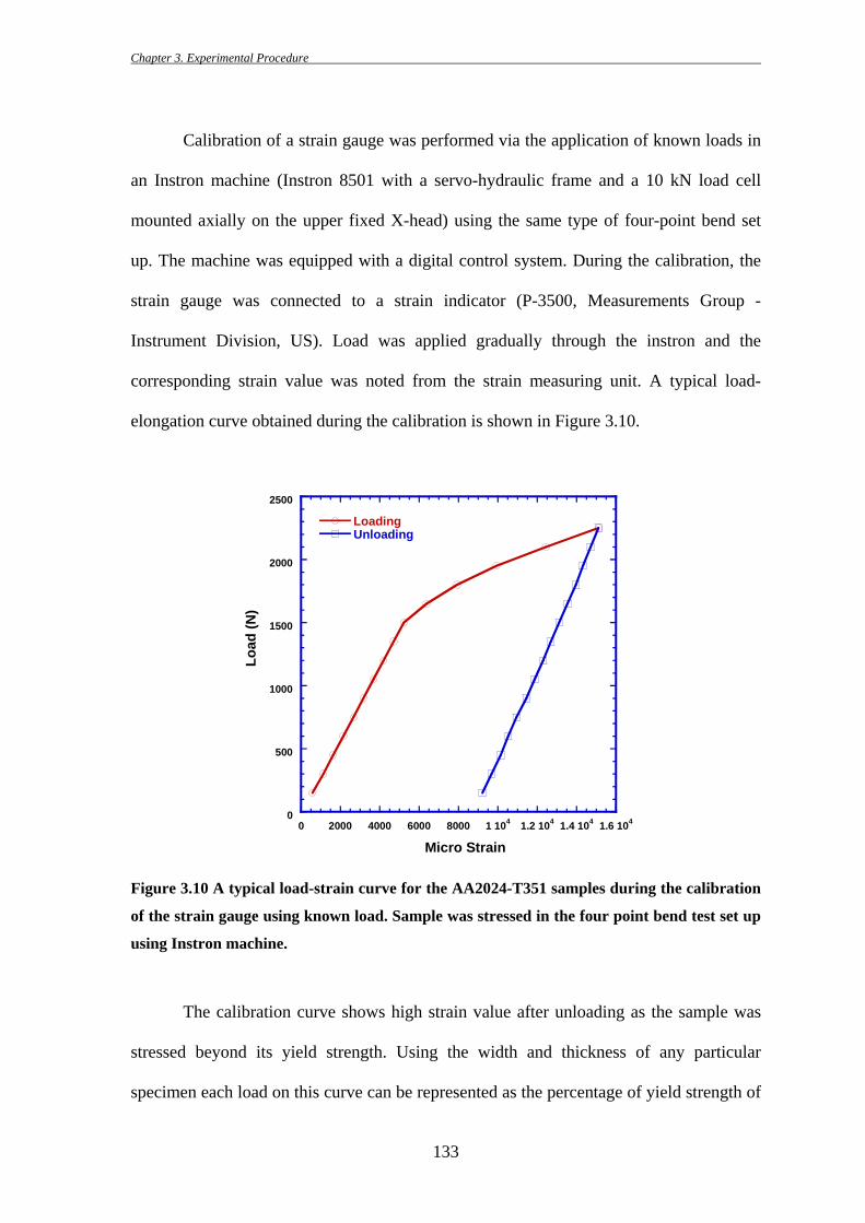
Calibration of a strain gauge was performed via the application of known loads in
an Instron machine (Instron 8501 with a servo-hydraulic frame and a 10 kN load cell
mounted axially on the upper fixed X-head) using the same type of four-point bend set
up. The machine was equipped with a digital control system. During the calibration, the
strain gauge was connected to a strain indicator (P-3500, Measurements Group -
Instrument Division, US). Load was applied gradually through the instron and the
corresponding strain value was noted from the strain measuring unit. A typical load-
elongation curve obtained during the calibration is shown in Figure 3.10.
Figure 3.10 A typical load-strain curve for the AA2024-T351 samples during the calibration
of the strain gauge using known load. Sample was stressed in the four point bend test set up
using Instron machine.
The calibration curve shows high strain value after unloading as the sample was
stressed beyond its yield strength. Using the width and thickness of any particular
specimen each load on this curve can be represented as the percentage of yield strength of
Chapter 3. Experimental Procedure
134
AA2024-T351. For example, using four-point bending stage geometry, load required to
reach the 90% of the yield strength (Y.S. ~375 MPa) for a particular AA2024-T351
sample was calculated to be about 1250N. The calibration curve showed the strain value
at this load as 4130e-06. During the in situ FEG-SEM experiments using the servo-
electric stressing stage, the sample was strained until the strain gauge output showed the
value of 4130e-06. This ensured any desired stress level in the specimens irrespective of
the load value read from the load cell.
3.6.3 FEG-SEM Observations Under In Situ Applied Stress
After the strain gauge was mounted on the specimen and silicone rubber was fully
cured, the specimen was loaded. It is important to measure the sample dimension prior to
its loading in the stage as any inaccurate measurement would result in to the wrong
calculation of load. Generally a strain gauge mounted on the sample surface and coated
with silicone rubber was left in air for 5-6 hours to ensure complete drying of the silicone
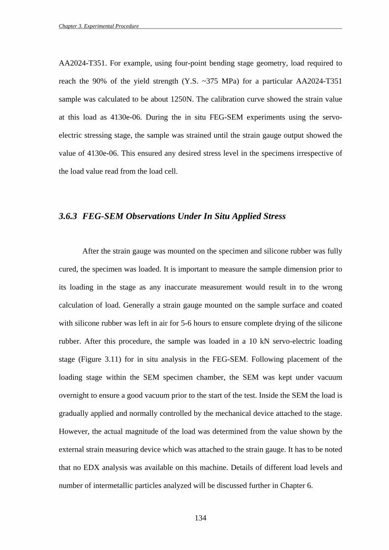
rubber. After this procedure, the sample was loaded in a 10 kN servo-electric loading
stage (Figure 3.11) for in situ analysis in the FEG-SEM. Following placement of the
loading stage within the SEM specimen chamber, the SEM was kept under vacuum
overnight to ensure a good vacuum prior to the start of the test. Inside the SEM the load is
gradually applied and normally controlled by the mechanical device attached to the stage.
However, the actual magnitude of the load was determined from the value shown by the
external strain measuring device which was attached to the strain gauge. It has to be noted
that no EDX analysis was available on this machine. Details of different load levels and
number of intermetallic particles analyzed will be discussed further in Chapter 6.
Chapter 3. Experimental Procedure
135
Figure 3.11 Four-point bend test set up with 10 KN servo electric loading stage.
3.7 Electrochemical Testing with an Applied Stress
3.7.1 Capillary Cell Electrochemical Studies Under Applied Plastic Stress
Using a 3-point Bend Set Up
Local electrochemical measurements in combination with a 3-point bending frame
were used to investigate the effect of applied plastic stress on the corrosion properties of
aluminium alloys. Local electrochemical measurements were performed on the L-T plane
of the wrought AA2024-T351 samples as well as on the cast Al-0.099Cu binary alloy.
AA2024-T351 samples were prepared in similar fashion as described for the four-point
bend in situ/SEM tests. The cast binary alloy was provided in the form of a 10 mm thick
plate. The top and bottom faces of the 10 mm thick plate was milled first and then
samples with 34.5 mm length, 10 mm width and 3 mm thickness were cut from it using
diamond blade cutter. All samples were polished to one micron diamond surface finish,
Specimen Instrumented Strain Gauge Four Point Bend Frame
Load Cell
Chapter 3. Experimental Procedure
136
rinsed in deionised water, ultrasonically cleaned in ethanol and dried prior to the test
following similar procedure described earlier.
Freshly polished sample shows some variability during the potentiodynamic scans
possibly due to the relatively unstable passive film on the surface. It was earlier reported
that leaving the polished sample in air for one day might bring some consistency in the
potentiodynamic scans in the unstressed condition [311]. This delay after polishing
ensures that the formation of the oxide film developing on the fresh metal surfaces has
reached its stable state. However, the delay after polishing do not influence the
conclusions derived from the potentiodynamic tests on unstressed vs. stressed samples.
Throughout this whole study, the time between the polishing and performing tests was
noted for each test.
Figure 3.12 shows the capillary cell electrochemical test set up. Except the
differences in the capillary, the capillary cell method is similar to that of the micro-
capillary electrochemical cell (as described in Section 3.5). Instead of a 40 µm diameter
glass capillary (as used in micro-capillary electrochemical cell - Section 3.5), an
approximately 1 mm diameter pipette (plastic pipette Finntip 60, supplied by Aldrich;
with an exposure area of 1.2 mm2) was used in the capillary cell used. The local cell
assembly (Figure 3.12) consisting of a pipette tip, a Pt wire counter electrode and
Ag/AgCl reference electrode was linked with a ‘GillAC’ ACM potentiostat or a “Field
Machine” potentiostat or a low noise potentiostat (CH Instruments, Model CHI600B).
Electrochemical tests were performed in naturally aerated 0.01 M or 0.1 M NaCl
solution at room temperature. Before the polarization, open circuit potential (OCP) of the
exposed area was monitored for 60-300 seconds. After the initial hold, anodic
polarization was started at a negative potential of 50 mV (i.e., 50 mV in the cathodic
domain) with respect to the OCP. Scan rate for all the experiments were 1 mV/s.
Chapter 3. Experimental Procedure
137
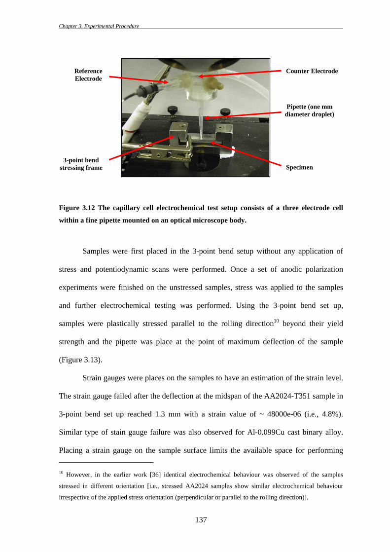
Figure 3.12 The capillary cell electrochemical test setup consists of a three electrode cell
within a fine pipette mounted on an optical microscope body.
Samples were first placed in the 3-point bend setup without any application of
stress and potentiodynamic scans were performed. Once a set of anodic polarization
experiments were finished on the unstressed samples, stress was applied to the samples
and further electrochemical testing was performed. Using the 3-point bend set up,
samples were plastically stressed parallel to the rolling direction10 beyond their yield
strength and the pipette was place at the point of maximum deflection of the sample
(Figure 3.13).
Strain gauges were places on the samples to have an estimation of the strain level.
The strain gauge failed after the deflection at the midspan of the AA2024-T351 sample in
3-point bend set up reached 1.3 mm with a strain value of ~ 48000e-06 (i.e., 4.8%).
Similar type of stain gauge failure was also observed for Al-0.099Cu cast binary alloy.
Placing a strain gauge on the sample surface limits the available space for performing 10 However, in the earlier work [36] identical electrochemical behaviour was observed of the samples
stressed in different orientation [i.e., stressed AA2024 samples show similar electrochemical behaviour
irrespective of the applied stress orientation (perpendicular or parallel to the rolling direction)].
Counter ElectrodeReference Electrode
Pipette (one mm diameter droplet)
Specimen 3-point bend
stressing frame
Chapter 3. Experimental Procedure
138
electrochemical experiments. So, to maintain the equivalent stress level for all the tests,
all samples were subjected to midspan deflection of 1.6 mm (i.e., strain > 5%). It should
be noted that, the strain level for the capillary cell electrochemical tests using 3-point
bend set up was much higher than the in situ FEG-SEM tests for particle delamination
using 4-point bend set up. The maximum strain in 4-point bend tests was 0.9% where as
in 3-point bend tests strain level was always > 5%.
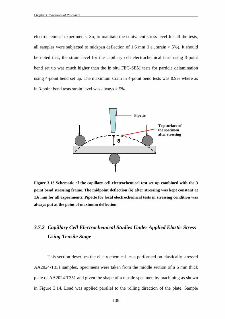
Figure 3.13 Schematic of the capillary cell electrochemical test set up combined with the 3
point bend stressing frame. The midpoint deflection (δ) after stressing was kept constant at
1.6 mm for all experiments. Pipette for local electrochemical tests in stressing condition was
always put at the point of maximum deflection.
3.7.2 Capillary Cell Electrochemical Studies Under Applied Elastic Stress
Using Tensile Stage
This section describes the electrochemical tests performed on elastically stressed
AA2024-T351 samples. Specimens were taken from the middle section of a 6 mm thick
plate of AA2024-T351 and given the shape of a tensile specimen by machining as shown
in Figure 3.14. Load was applied parallel to the rolling direction of the plate. Sample
δδ
Pipette
Top surface of the specimen after stressing
Chapter 3. Experimental Procedure
139
preparation and the local electrochemistry set up (capillary cell, exposed area ~ 1.2 mm2)
were similar to that of described in Section 3.7.1. All measurements included in this
section were performed using a low noise potentiostat (CH Instruments, Model
CHI600B). AA2024-T351 specimens were stored in air at least one day after polishing to
ensure a stable passive film on the specimen surface.
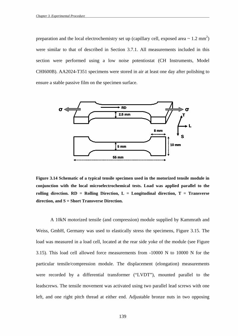
Figure 3.14 Schematic of a typical tensile specimen used in the motorized tensile module in
conjunction with the local microelectrochemical tests. Load was applied parallel to the
rolling direction. RD = Rolling Direction, L = Longitudinal direction, T = Transverse
direction, and S = Short Transverse Direction.
A 10kN motorized tensile (and compression) module supplied by Kammrath and
Weiss, GmbH, Germany was used to elastically stress the specimens, Figure 3.15. The
load was measured in a load cell, located at the rear side yoke of the module (see Figure
3.15). This load cell allowed force measurements from -10000 N to 10000 N for the
particular tensile/compression module. The displacement (elongation) measurements
were recorded by a differential transformer (“LVDT”), mounted parallel to the
leadscrews. The tensile movement was activated using two parallel lead screws with one
left, and one right pitch thread at either end. Adjustable bronze nuts in two opposing
2.5 mm
10 mm
8 mm
5 mm
55 mm
RDσ σT
L
S
2.5 mm
10 mm
8 mm
5 mm
55 mm
RDσ σ2.5 mm
10 mm
8 mm
5 mm
55 mm
RD
2.5 mm
10 mm
8 mm
5 mm
55 mm
RDσ σT
L
S
T
L
S
Chapter 3. Experimental Procedure
140
“yokes” bear these leadscrews, and applied the force evenly. A DC motor and two sets of
worm gears applied the downgeared main shaft rotation. This resulted in a self-locking
mechanism of high rigidity, where the experiment forces were all enclosed in the
rectangular load frame. One of the advantages of this design is the fact that both yokes
apply the movement equally to both sides of the specimen. The tensile module was
controlled by the DDS controller/microprocessor supplied with the module. This
controller can be operated independently or through a computer using DDS software. The
microprocessor provided pre-selected displacement speed over a range of 0.1 µm/s to 20
µm/s.
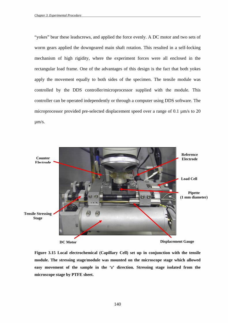
Figure 3.15 Local electrochemical (Capillary Cell) set up in conjunction with the tensile
module. The stressing stage/module was mounted on the microscope stage which allowed
easy movement of the sample in the ‘z’ direction. Stressing stage isolated from the
microscope stage by PTFE sheet.
Load Cell
Displacement Gauge DC Motor
Reference Electrode
Pipette (1 mm diameter)
Counter Electrode
Tensile Stressing Stage
Chapter 3. Experimental Procedure
141
The most important factor while performing these experiments was to make sure
that the specimen was completely isolated from the tensile stage, specially from the load
cell. Any contact of the specimen with the stressing stage made it impossible to perform
any electrochemical tests as the stage itself acted as a source of constant current. So, first
the stressing stage was isolated from the microscope stage using a non-conductive PTFE
sheet. The specimens were normally held by a metal grip in the stressing stage. These
grips were made from Zircaloy and then heat treated for 12 hrs at 650˚C. This heat
treatment formed a thick and non-conductive oxide layer on the surface of the grips. Use
of these grips during the tests ensured complete isolation of the test specimen.
Before putting the specimen in the stressing stage, the load and elongation value
of the set up was brought to zero using the microprocessor control. The thickness and the
width of the specimens were measured carefully before mounting them in the stressing
stage. The screws used for tightening the grips were also covered using PTFE tape to
ensure electrical isolation of the specimen. Complete isolation of the specimen was
checked repeatedly using a hand held voltmeter. Normally after tightening the screws on
the specimen, load value showed a negative value. Load value was brought to zero using
the stress stage controls. Based on the sample cross section, the desired load (in N) was
calculated as a fraction of yield stress of AA2024-T351. For example, an AA2024-T351
specimen with a cross section of 12.5 mm2 was calculated to need about 3280 N (i.e., 375
× 12.5 × 0.7) of load for stressing to 70% of its yield stress (as yield stress of AA2024-
T351 is 375 MPa). In this current study tests on AA2024-T351 specimens were carried
out at a stress level of 45%, 70%, and 90% of its yield strength. Stress was assumed to be
distributed uniformly through out the specimen in the elastic region.
Electrochemical tests of the unstressed specimen were performed at the areas
slightly far from the middle of the specimen. Once the experiments were completed on
Chapter 3. Experimental Procedure
142
the specimen in the unstressed condition, the specimen was stressed to the pre-calculated
load. Displacement speed during the stressing was kept between 2-5 µm/s. The software
simultaneously gave the load (N) vs. time (s) curve or load (N) vs. elongation (µm) curve.
The tensile module was used in two ways for keeping the load constant at the desired
level. After reaching to the pre-calculated load, the motor was stopped and hence the
sample stayed at that particular load. However, there was also a ‘constant load’ option
with the tensile module which allows the specimens to be kept at a particular load. Load
was monitored as a function of time during the course of experiments. In few occasions a
40-50 N decrease in the load had been observed over a period of 3-4 hours. Any further
decrease in the load was compensated by stressing the specimen again to the original
value. Once the tests were completed, the specimen was brought back to zero load and
taken out of the stressing module.
All experiments on AA2024-T351 to find out the effect of elastic stress were
performed in naturally aerated 0.01 M NaCl at room temperature. Before the polarization,
the open circuit potential (OCP) of the exposed area was monitored for 60-300 seconds.
After the initial hold, anodic polarization was started at a negative potential of 50 mV
(i.e., 50 mV in the cathodic domain) with respect to the OCP. Potentiodynamic scans
were performed in similar fashion as it was described in Section 3.7.1 (i.e., at a scan rate
of 1 mV/s).
As the potentiodynamic scans were not conclusive enough to find out the effect of
low applied elastic stresses (i.e., 45% and 70% Y.S.) on the corrosion properties
(corrosion and breakdown potentials, passive current densities etc.) of the AA2024-T351
specimens, effect of applied stress was further investigated using a potentiostatic
polarization technique and calculating the charge passed within a defined time span.
According to Faraday’s Law, the higher the dissolution of the exposed material, the
Chapter 3. Experimental Procedure
143
higher the amount of charge passed. During the potentiostatic tests, data was collected in
the form of current (A) vs. time (s) through the software controlling the CHI600B
potentiostat. Data collection frequency was set at 10 Hz. After the completion of the test,
collected data was converted into text format and analysed by a commercial software
named ‘KaleidaGraph (version 4.0)’. Current passed during the tests was converted to
current density depending on the exposed area (~1.2 mm2 in this case) and plotted as a
function of time (s). As the charge in coulomb (C) is represented by the multiplication of
current in ampere (A) with time in second (s), the KaleidaGraph software was used to
integrate the current (A) vs. time (s) plot obtained from the potentiostatic test. The
KaleidaGraph software was used to run a macro for calculating the indefinite integral,
yielding a new curve. This macro found the incremental area under the curve, given the
X-Y data points [in this case time (s) and current (A)] describing the curve. Integration of
the current density (A/cm2) vs. time (s) plot resulted in a new curve with charge density
(C/cm2) vs. time (s). Each point on this curve indicated the density of the total charge
passed until that time during the experiment.
3.7.3 Micro-Capillary Electrochemical Cell Studies Under Applied
Elastic/Plastic Stress Using Tensile Stage
This section describes the micro-capillary electrochemical cell (with an exposed
area of 40 µm diameter) tests performed on the elastically/plastically stressed AA2024-
T351 samples. Specimens were taken from the middle section of a 6 mm thick plate of
AA2024-T351 and given the shape of a double notch flat tensile specimen with two
semicircular notches at the middle by machining. The typical shape and dimension of
Chapter 3. Experimental Procedure
144
such tensile specimen is shown in Figure 3.16. Load was applied perpendicular to the
rolling direction of the plate. Sample preparation and the local electrochemical set up
were similar to that of described in Section 3.7.2. Apart from the specimen shape, the
main difference between these two sections is that, in this current section, a capillary
diameter of 40 µm was used instead of 1 mm diameter pipette (as used in Section 3.7.2).
As the same 10kN motorized tensile (and compression) module supplied by Kammrath
and Weiss, GmbH, Germany was used in both cases to stress the specimens, the specimen
mounting on the stressing stage and operating procedure were similar. The small
exposure area of this technique allowed the possibility of performing a series of
electrochemical tests as a function of stress on a particular notched specimen with a stress
distribution (both elastic and plastic) around the notch.
A numerical simulation based on the finite element method was performed to
calculate the surface stress on notched tensile AA2024-T351 specimens (schematic of
such specimen is shown in Figure 3.16).11 QUA4 elements composed of four nodes
located at the four geometric corners of quadrangles were used in the meshing and the
density of elements was chosen such that the size of an element was around 1 µm. The
different equations and the conventions used in the mechanical analysis can be found
elsewhere [312]. The matrix was assumed to behave like an isotropic elastic-plastic
medium (E = 83 GPa and n = 0.33). The elastic-plastic material model used for the matrix
was determined by fitting an experimental stress-strain curve (as described in Section
3.6.1) with the finite-element method model. The surface stress field was calculated under
constant loading conditions. Stress distribution around the semicircular notch at the
middle of the specimen varied depending on the applied global stress. The applied global 11 Numerical analysis was performed by Vincent Vignal from LRRS, Université de Bourgogne, Dijon,
France as a part of an International collaboration funded by the Royal Society, UK.
Chapter 3. Experimental Procedure
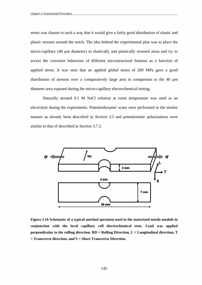
145
stress was chosen in such a way that it would give a fairly good distribution of elastic and
plastic stresses around the notch. The idea behind the experimental plan was to place the
micro-capillary (40 µm diameter) in elastically and plastically stressed areas and try to
access the corrosion behaviour of different microstructural features as a function of
applied stress. It was seen that an applied global stress of 200 MPa gave a good
distribution of stresses over a comparatively large area in comparison to the 40 µm
diameter area exposed during the micro-capillary electrochemical testing.
Naturally aerated 0.1 M NaCl solution at room temperature was used as an
electrolyte during the experiments. Potentiodynamic scans were performed in the similar
manner as already been described in Section 3.5 and potentiostatic polarizations were
similar to that of described in Section 3.7.2.
Figure 3.16 Schematic of a typical notched specimen used in the motorized tensile module in
conjunction with the local capillary cell electrochemical tests. Load was applied
perpendicular to the rolling direction. RD = Rolling Direction, L = Longitudinal direction, T
= Transverse direction, and S = Short Transverse Direction.
4 mm
7 mm
55 mm
2 mm
RDσ σL
T
S4 mm
7 mm
55 mm
2 mm
RDσ σ
4 mm
7 mm
55 mm
2 mm
RD
4 mm
7 mm
55 mm
2 mm
RDσ σL
T
S
L
T
S
Chapter 3. Experimental Procedure
146
TS
LRD
TS
LRD
3.8 X-Ray Synchrotron Tomography
3.8.1 Sample Preparation for the Synchrotron Studies
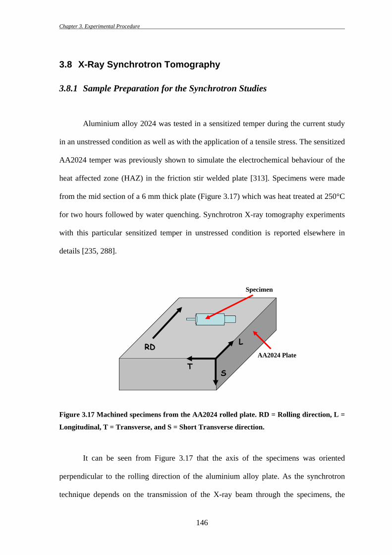
Aluminium alloy 2024 was tested in a sensitized temper during the current study
in an unstressed condition as well as with the application of a tensile stress. The sensitized
AA2024 temper was previously shown to simulate the electrochemical behaviour of the
heat affected zone (HAZ) in the friction stir welded plate [313]. Specimens were made
from the mid section of a 6 mm thick plate (Figure 3.17) which was heat treated at 250°C
for two hours followed by water quenching. Synchrotron X-ray tomography experiments
with this particular sensitized temper in unstressed condition is reported elsewhere in
details [235, 288].
Figure 3.17 Machined specimens from the AA2024 rolled plate. RD = Rolling direction, L =
Longitudinal, T = Transverse, and S = Short Transverse direction.
It can be seen from Figure 3.17 that the axis of the specimens was oriented
perpendicular to the rolling direction of the aluminium alloy plate. As the synchrotron
technique depends on the transmission of the X-ray beam through the specimens, the
Specimen
AA2024 Plate
Chapter 3. Experimental Procedure
147
specimen size was dictated by the incident beam energy and several other parameters
(i.e., X-ray scintillator efficiency, signal to noise ration etc.) of the beam line set up. Both
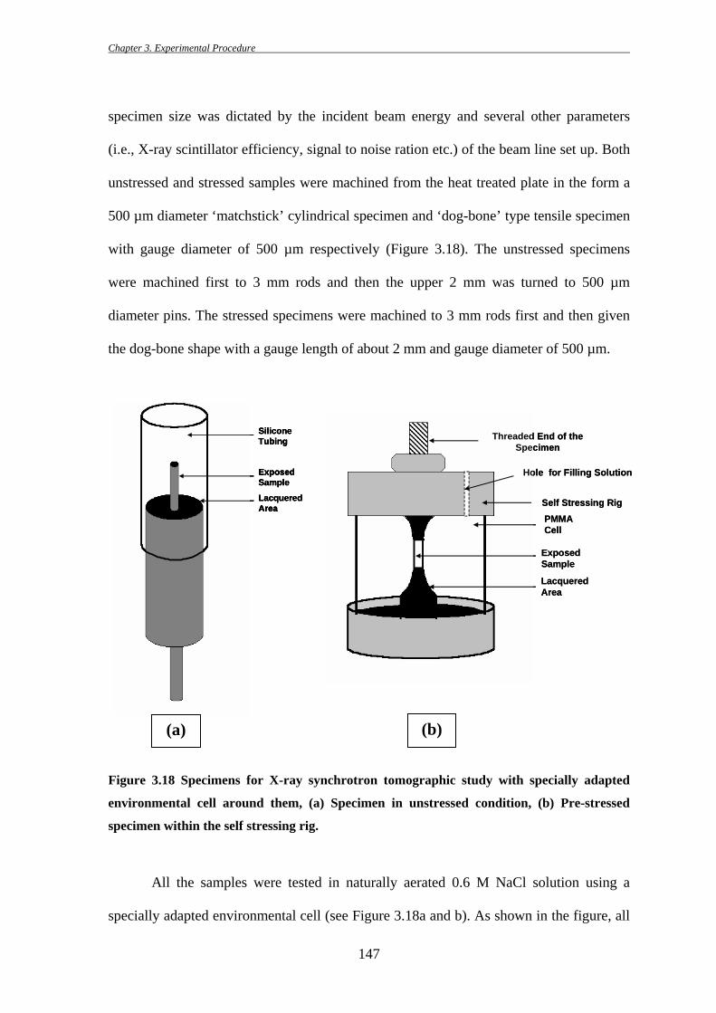
unstressed and stressed samples were machined from the heat treated plate in the form a
500 µm diameter ‘matchstick’ cylindrical specimen and ‘dog-bone’ type tensile specimen
with gauge diameter of 500 µm respectively (Figure 3.18). The unstressed specimens
were machined first to 3 mm rods and then the upper 2 mm was turned to 500 µm
diameter pins. The stressed specimens were machined to 3 mm rods first and then given
the dog-bone shape with a gauge length of about 2 mm and gauge diameter of 500 µm.
Figure 3.18 Specimens for X-ray synchrotron tomographic study with specially adapted
environmental cell around them, (a) Specimen in unstressed condition, (b) Pre-stressed
specimen within the self stressing rig.
All the samples were tested in naturally aerated 0.6 M NaCl solution using a
specially adapted environmental cell (see Figure 3.18a and b). As shown in the figure, all
Silicone Tubing
Exposed Sample
LacqueredArea
Silicone Tubing
Exposed Sample
LacqueredArea
Silicone Tubing
Exposed Sample
LacqueredArea Self Stressing Rig
PMMA Cell
Exposed Sample
LacqueredArea
Hole for Filling Solution
Threaded End of the Specimen
Self Stressing RigPMMA Cell
Exposed Sample
LacqueredArea
Hole for Filling Solution
Threaded End of the Specimen
(a) (b)
Chapter 3. Experimental Procedure
148
samples (both unstressed and stressed specimens) were lacquered with Stopping Off
Lacquer to avoid any unwanted material exposure or crevicing. Silicone tubing and
PMMA polymer was used around the unstressed and stressed sample respectively to form
the environmental cell. Dog bone tensile specimens with 500 µm diameters were stressed
to 70% and 90% of the yield stress (yield stress of sensitized temper AA2024 was
determined to be about 375 MPa from the average of two repeat experiments) prior to the
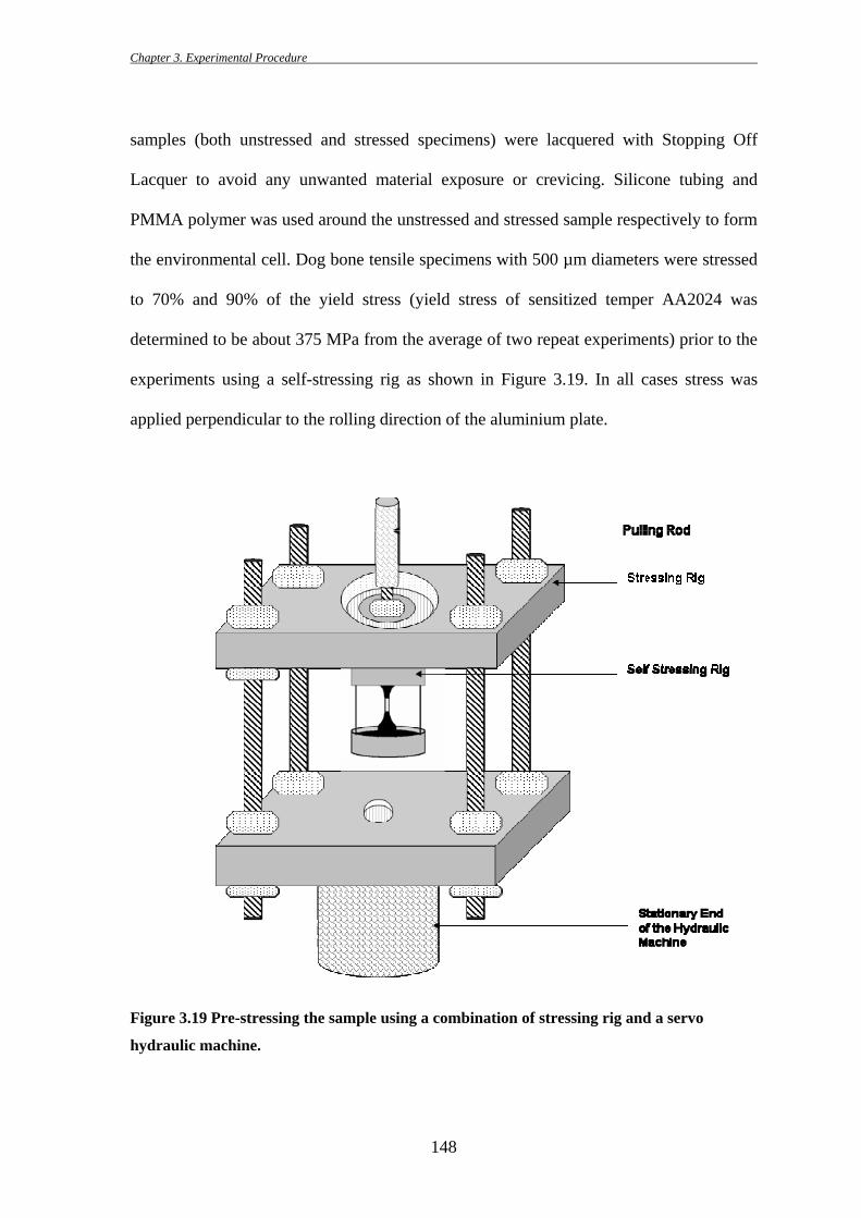
experiments using a self-stressing rig as shown in Figure 3.19. In all cases stress was
applied perpendicular to the rolling direction of the aluminium plate.
Figure 3.19 Pre-stressing the sample using a combination of stressing rig and a servo
hydraulic machine.
Chapter 3. Experimental Procedure
149
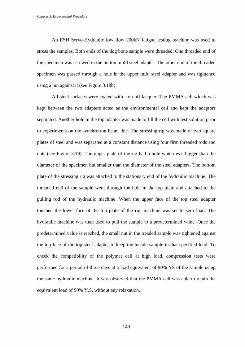
An ESH Servo-Hydraulic low flow 200kN fatigue testing machine was used to
stress the samples. Both ends of the dog bone sample were threaded. One threaded end of
the specimen was screwed in the bottom mild steel adapter. The other end of the threaded
specimen was passed through a hole in the upper mild steel adapter and was tightened
using a nut against it (see Figure 3.18b).
All steel surfaces were coated with stop off lacquer. The PMMA cell which was
kept between the two adapters acted as the environmental cell and kept the adaptors
separated. Another hole in the top adapter was made to fill the cell with test solution prior
to experiments on the synchrotron beam line. The stressing rig was made of two square
plates of steel and was separated at a constant distance using four firm threaded rods and
nuts (see Figure 3.19). The upper plate of the rig had a hole which was bigger than the
diameter of the specimen but smaller than the diameter of the steel adapters. The bottom
plate of the stressing rig was attached to the stationary end of the hydraulic machine. The
threaded end of the sample went through the hole in the top plate and attached to the
pulling rod of the hydraulic machine. When the upper face of the top steel adapter
touched the lower face of the top plate of the rig, machine was set to zero load. The
hydraulic machine was then used to pull the sample to a predetermined value. Once the
predetermined value is reached, the small nut in the treaded sample was tightened against
the top face of the top steel adapter to keep the tensile sample in that specified load. To
check the compatibility of the polymer cell at high load, compression tests were
performed for a period of three days at a load equivalent of 90% YS of the sample using
the same hydraulic machine. It was observed that the PMMA cell was able to retain the
equivalent load of 90% Y.S. without any relaxation.
Chapter 3. Experimental Procedure
150
3.8.2 Synchrotron Experiments in the Beam Line and the Reconstruction
Procedure
In situ12 Synchrotron tomographic experiments were performed on the Materials
Science beam line X04SA at the Swiss Light Source (SLS), Paul Scherrer Institute, in
Switzerland [262] to quantify the effect of applied stress on the propagation of localized
corrosion (IGC) as a function of time. Tomographic scans were performed on unstressed
and stressed AA2024 (sensitized temper) specimens exposed to 0.6 M NaCl solution at
room temperature at open circuit. Times for each tomographic scans were between 40 and
60 min in duration. A sequence of tomographic scans was then performed on each
specimen at certain interval during the exposure up to a maximum of two days. As
described earlier (see Figure 3.18a and b), the environmental cell around the specimens
were filled, at the beam line, with solution before the start of the first scan of respective
specimens. Deionized water was added to the environmental cell whenever necessary
during the exposure to compensate the solution loss due to evaporation.
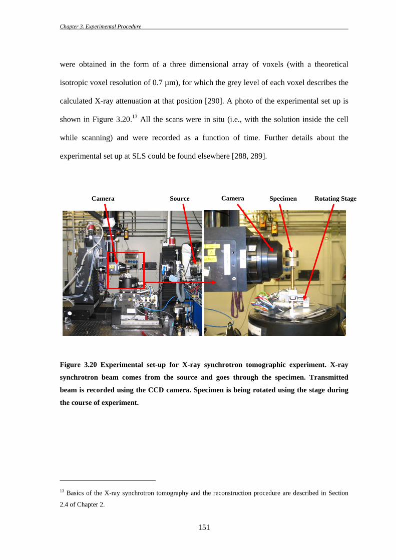
The energy of the monochromatic X-ray beam was set to 17.5 keV. The distance
between the sample and the CCD camera detector was 30 mm (Figure 3.20). The X-ray
detector system optics were set up so that the radiographic images were magnified by 40x
between the scintillator and the CCD camera, which was set to acquire 1024 × 1024
pixels of data. During the 180° rotation of the sample (using a 0.3 s exposure/projection),
a series of 1023 radiographs (2D) were taken. The recorded radiographs were
reconstructed to 3D volumes using filtered back projection algorithm [314]. The data
12 During the in situ experiments, specimens within the environmental cell (i.e., specimens immersed in the
corrosive solution) were placed in the synchrotron beam line for tomographic scan. This technique allowed
real time monitoring of the corrosion process.
Chapter 3. Experimental Procedure
151
were obtained in the form of a three dimensional array of voxels (with a theoretical
isotropic voxel resolution of 0.7 µm), for which the grey level of each voxel describes the
calculated X-ray attenuation at that position [290]. A photo of the experimental set up is
shown in Figure 3.20.13 All the scans were in situ (i.e., with the solution inside the cell
while scanning) and were recorded as a function of time. Further details about the
experimental set up at SLS could be found elsewhere [288, 289].
Figure 3.20 Experimental set-up for X-ray synchrotron tomographic experiment. X-ray
synchrotron beam comes from the source and goes through the specimen. Transmitted
beam is recorded using the CCD camera. Specimen is being rotated using the stage during
the course of experiment.
13 Basics of the X-ray synchrotron tomography and the reconstruction procedure are described in Section
2.4 of Chapter 2.
Camera Specimen Rotating StageCamera Source
Chapter 3. Experimental Procedure
152
3.8.3 3D Visualization and Analysis of the Tomographic Data
Visualization and 3D analysis of the tomography data from the synchrotron
experiments were performed using the commercial 3D visualization and modelling
software ‘Amira’. Using this software, two dimensional tomographs were combined
together to provide a 3D representation of the corrosion attack morphology and its
interaction with the alloy microstructure.
Reconstructed raw data (in the “rec.DMP” format) were directly loaded into the
software as a stack of 2D slices. Various data processing modules (e.g., contrast control)
helped in simple and efficient manipulation of the image. The image segment editor14 of
this particular software (i.e., ‘Amira’) was used to label voxels corresponding to the alloy
matrix, intermetallic particles and corrosion based the differences in their contrast values.
The labelled regions of each specimen were then represented in three dimensions (3D) as
triangular surface grids suitable for numerical analysis and simulations. Different features
(e.g., corrosion attacks, alloy matrix) were labelled in different colours and the specimen
matrix material has been rendered translucent in order to observe the morphology of
corrosion attacks within the interior of the specimen. With the input of voxel sizes in 3D
space (i.e., 0.7 µm in x, y, and z axis in this case), quantitative analysis of the labelled
regions were performed.
Volume of both the corrosion attacks and the samples exposed during the
tomographic scans were calculated using the software. Based on these calculations,
growth rate of corrosion attacks as a function of exposure time were expressed as volume
of metal loss as a percentage of specimen volume (see Chapter 7).
14 Segmentation is a process of dividing an image data into different segments for 3D model reconstruction.
Chapter 4. Effect of Surface Treatment and Its Beneficial Effect on the Corrosion Properties of AA2024-T351
153
4 EFFECT OF SURFACE TREATMENT AND ITS
BENEFICIAL EFFECT ON THE CORROSION
PROPERTIES OF AA2024-T351
High strength aluminium alloy 2024-T351 is susceptible to localized corrosion in
the forms of pitting and intergranular corrosion, which can be potential sites for initiation
of cracks and thereby could result in catastrophic failure. Two predominant categories of
second-phase intermetallic particles have been identified in AA2024-T3: elongated or
irregular shaped Al-Cu-Fe-Mn containing particles [Al6(CuFeMn) or with other
stoichiometric relationships; in short they will be termed as “Fe-Mn” particle throughout
this study] which are generally believed to act as cathode during the corrosion process
[7-9, 11, 175, 186, 187, 191] and ‘S’ (Al2CuMg) phase intermetallic particles which show
initial anodic behaviour during the corrosion process. However, dealloying of ‘S’ phase
particles can then lead to Cu enrichment on the particles and make them cathodically
active. Hence, ‘S’ phase particles are thought to be the key contributor for the poor
corrosion resistance of AA2024 [8, 12, 14, 37, 40, 43, 46, 174, 185, 198].
The key purpose of this study is to examine the effectiveness of a surface
treatment technique in removing deleterious ‘S’ phase particles from the surface and
thereby improving the corrosion properties of AA2024-T351. The effects of ‘S’ phase
particle removal on the initiation of localized corrosion in AA2024-T351 have been
investigated using several electrochemical techniques during this present study.
Chapter 4. Effect of Surface Treatment and Its Beneficial Effect on the Corrosion Properties of AA2024-T351
154
4.1 Microstructural Characterization of AA2024-T351
Scanning Electron Microscopic (SEM) analysis of polished AA2024-T351 was
performed in both high low and high magnification to reveal the general microstructure as
well as the morphology of the individual intermetallic particles. EDS spectrums were use
to quantify the composition of each types of intermetallic particles and the base metal
matrix. Figure 4.1(a) shows the general microstructure of AA2024-T351 base metal
surface as revealed by low magnification SEM micrographs. The presence of a large
number of constituent intermetallic particles can easily be seen from the micrographs.
Sometimes the intermetallic particles are formed as clusters and after cold rolling they
break up and often align parallel to the rolling direction. Figure 4.1(a) also shows the
presence of some pre-existing hole or pores in the sample. Presence of such holes/pores in
the AA2024-T351 had also been confirmed using synchrotron studies and will be
discussed later in Chapter 7. EDS analysis showed that the matrix of AA2024-T351
mainly consists of ~ 93 wt% Al, ~ 1.2 wt% Mg, ~ 4 wt% Cu with small amount of
impurity element like Fe, Mn and Si.
4.1.1 The Intermetallic Particles
Two predominant categories of coarse intermetallic particles have been identified
in the microstructure as shown in Figure 4.1(b) and Figure 4.1(c). The first type is
irregular in shape and in the size range of 10-20 µm containing mainly Fe-Mn-Cu-Al
(Figure 4.1b). In very few occasions these Fe-containing intermetallic particles are found
to contain Si.
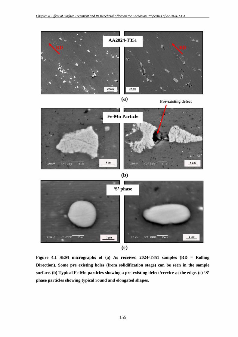
Chapter 4. Effect of Surface Treatment and Its Beneficial Effect on the Corrosion Properties of AA2024-T351
155
Figure 4.1 SEM micrographs of (a) As received 2024-T351 samples (RD = Rolling
Direction). Some pre existing holes (from solidification stage) can be seen in the sample
surface. (b) Typical Fe-Mn particles showing a pre-existing defect/crevice at the edge. (c) ‘S’
phase particles showing typical round and elongated shapes.
(b)
(a)
(c)
AA2024-T351
Fe-Mn Particle
‘S’ phase
Pre-existing defect
RD RD
Chapter 4. Effect of Surface Treatment and Its Beneficial Effect on the Corrosion Properties of AA2024-T351
156
These particles are sometimes found to be broken into fragments during the
subsequent thermo-mechanical treatment as they are harder than the matrix. This is
consistent with the findings of others [7, 8, 81]. Pre-existing defects/crevices at the edge
of Fe-containing particles are also found in several occasions (e.g. Figure 4.1b; further
SEM and AFM analysis of such pre-existing defects can be found in Chapter 6) which is
consistent with the observations of other researcher [235]. By comparison, the second
types of coarse intermetallic particles containing Al-Cu-Mg are rounded and smooth in
appearance within the size range of 2-5 µm (Figure 4.1c,). In a few cases these Al-Cu-Mg
particles are found to be in an elongated shape and as large as ~ 10 µm in size. A small
number of rounded and smooth particles are seen to contain Al and Cu. However, the
numbers of Fe-containing particles having Si and Al-Cu particles are insignificant
compared to the Fe-Mn-Cu-Al particles or Al-Cu-Mg particles. So, this study will
primarily be focused on Fe-Mn-Cu-Al and Al-Cu-Mg intermetallic particles. Typical
examples of EDS spectra of different types of intermetallic particles are shown in Figure
4.2. Compositional analysis of the two predominant types of intermetallic particles is
shown in Table 4.1. Forty different particles of each type (ten particles each from four
different AA2024-T351 samples) were analysed and the elemental compositional mean
with their standard deviation were calculated. Table 4.1 shows the weight and atomic
percentage of each element in different intermetallics.
The Al-Cu-Mg particles in AA2024 have been reported as Al2CuMg or ‘S’ phase
by several authors [5-9, 11, 19, 43-45, 70, 76, 80, 174, 198, 204, 211, 315]. It can clearly
be seen from Table 4.1 that Al-Cu-Mg particles of this study closely follow the
stoichiometric composition of Al2CuMg and hence can be assigned as ‘S’ phase. As
stated earlier, Al-Cu particles are less often observed in AA2024 compared to ‘S’ phase
particles.
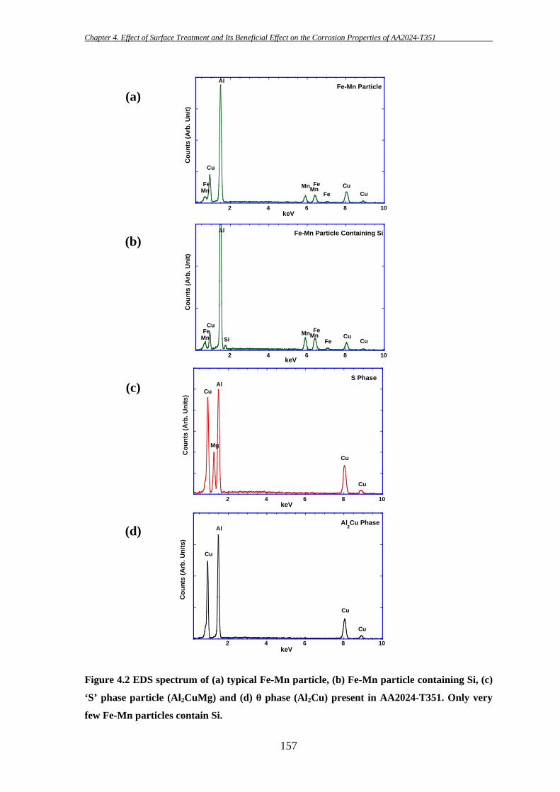
Chapter 4. Effect of Surface Treatment and Its Beneficial Effect on the Corrosion Properties of AA2024-T351
157
Figure 4.2 EDS spectrum of (a) typical Fe-Mn particle, (b) Fe-Mn particle containing Si, (c)
‘S’ phase particle (Al2CuMg) and (d) θ phase (Al2Cu) present in AA2024-T351. Only very
few Fe-Mn particles contain Si.
(a)
(b)
(c)
(d)
2 4 6 8 10
Cou
nts
(Arb
. Uni
t)
keV
Mn
Al
CuCu
Cu
MnFe
FeMnFe
Fe-Mn Particle
2 4 6 8 10
Cou
nts
(Arb
. Uni
t)
keV
Mn
Al
CuCu
CuMnFe
FeMnFe
Si
Fe-Mn Particle Containing Si
2 4 6 8 10
Cou
nts
(Arb
. Uni
ts)
keV
Mg
Al
Cu
Cu
Cu
S Phase
2 4 6 8 10
Cou
nts
(Arb
. Uni
ts)
keV
Al
Cu
Cu
Cu
Al2Cu Phase

Chapter 4. Effect of Surface Treatment and Its Beneficial Effect on the Corrosion Properties of AA2024-T351
158
Table 4.1 Composition (Weight and Atomic % ± Standard Deviation) of intermetallic
particles in AA2024-T351
Element Al Cu Mg Fe Mn
Wt.% At.% Wt.% At.% Wt.% At.% Wt.% At.% Wt.% At.%
‘S’ phase 41.3 ± 3.5
54 ± 3.5
44 ± 3.7
24.7 ± 2.8
14.5 ± 2
21 ± 2.7 - - - -
Fe-Mn Particle
55.6 ± 3.3
73.6 ± 2.4
27.9 ± 5.5
15.8 ± 3.4 - - 7.8
± 1.2 5
± 0.9 8.8
± 3.3 5.7 ± 2
In this present study the Al-Cu particles are found to consist of Al (wt% ~ 48.4±2,
at% ~ 68.8±1.8) and Cu (wt% ~ 51.6±2, at% ~ 31.2±1.8). So, from the stoichiometric
relationship the Al-Cu particles could be assigned as Al2Cu and is consistent with the
findings of other researchers [75]. These Al2Cu particles are small, rounded (1-2 µm) and
generally found as isolated individual particles.
However, the Fe-containing intermetallic particles from this present study seem to
follow a stoichiometric relationship close to Al15Cu3(Fe,Mn). Several compositions of Fe-
containing intermetallic particles have been reported in the literature, Al6(CuFeMn) [9,
11], Cu2AlFe7 [9, 73, 204], Al7Cu2(Fe,Mn) [76], (Fe,Mn)xSi(Al,Cu)y [75, 78]. A very few
Fe-containing intermetallic particles in this current study have been found to contain
significant amounts of Si. Only one particle (among the 40 Fe-containing particles
analyzed) showed the presence of ~2 wt% of Si. So, the current study emphasize the fact
as pointed out by other researchers [7, 75] that the Fe-containing intermetallic particles in
AA2024 may not always possess a particular and definite stoichiometric relationship.
Hence the Fe-rich intermetallic particles will be referred as Fe-Mn particles/phase in this
current study.
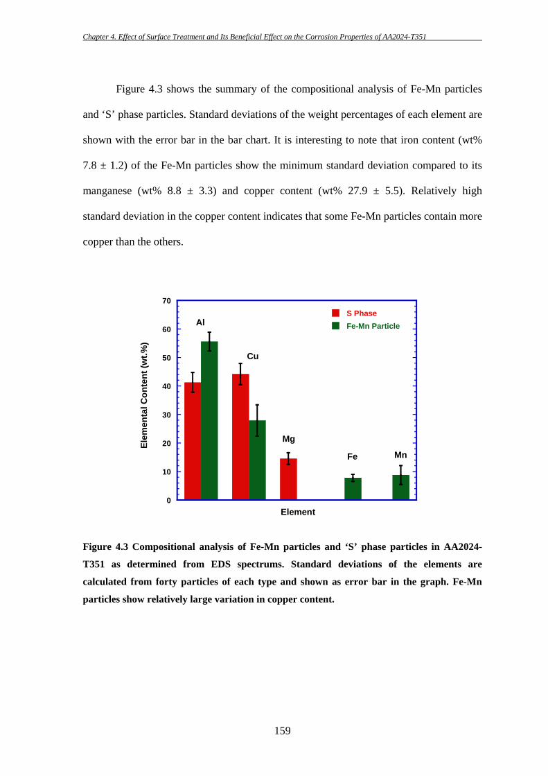
Chapter 4. Effect of Surface Treatment and Its Beneficial Effect on the Corrosion Properties of AA2024-T351
159
0
10
20
30
40
50
60
70S Phase Fe-Mn Particle
Elem
enta
l Con
tent
(wt.%
)
Element
Al
Cu
Mg
Fe Mn
Figure 4.3 shows the summary of the compositional analysis of Fe-Mn particles
and ‘S’ phase particles. Standard deviations of the weight percentages of each element are
shown with the error bar in the bar chart. It is interesting to note that iron content (wt%
7.8 ± 1.2) of the Fe-Mn particles show the minimum standard deviation compared to its
manganese (wt% 8.8 ± 3.3) and copper content (wt% 27.9 ± 5.5). Relatively high
standard deviation in the copper content indicates that some Fe-Mn particles contain more
copper than the others.
Figure 4.3 Compositional analysis of Fe-Mn particles and ‘S’ phase particles in AA2024-
T351 as determined from EDS spectrums. Standard deviations of the elements are
calculated from forty particles of each type and shown as error bar in the graph. Fe-Mn
particles show relatively large variation in copper content.
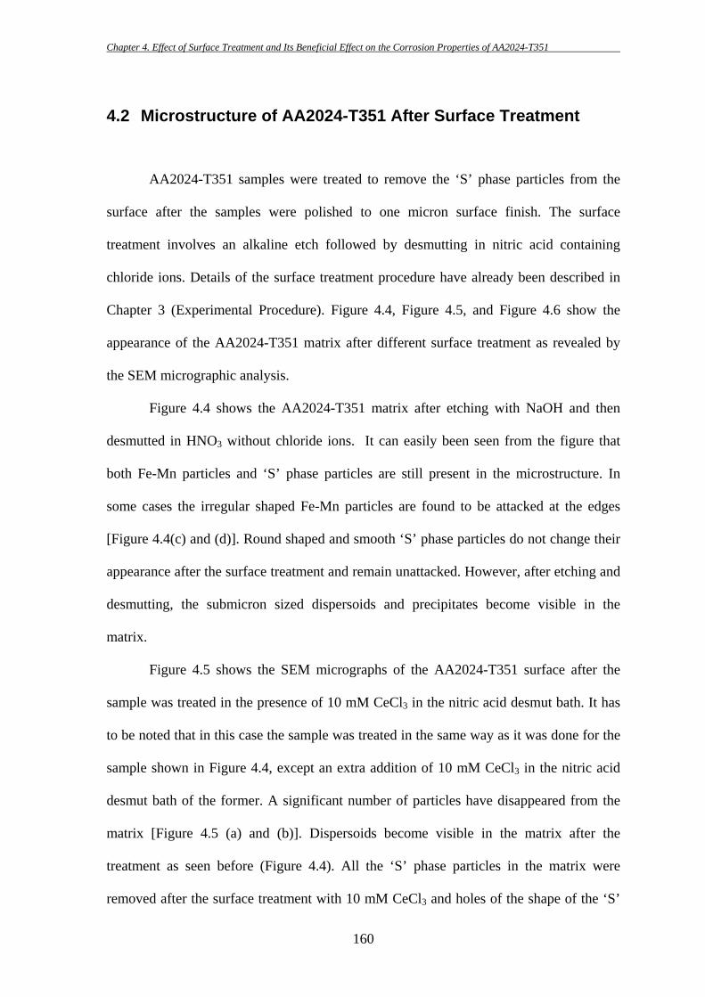
Chapter 4. Effect of Surface Treatment and Its Beneficial Effect on the Corrosion Properties of AA2024-T351
160
4.2 Microstructure of AA2024-T351 After Surface Treatment
AA2024-T351 samples were treated to remove the ‘S’ phase particles from the
surface after the samples were polished to one micron surface finish. The surface
treatment involves an alkaline etch followed by desmutting in nitric acid containing
chloride ions. Details of the surface treatment procedure have already been described in
Chapter 3 (Experimental Procedure). Figure 4.4, Figure 4.5, and Figure 4.6 show the
appearance of the AA2024-T351 matrix after different surface treatment as revealed by
the SEM micrographic analysis.
Figure 4.4 shows the AA2024-T351 matrix after etching with NaOH and then
desmutted in HNO3 without chloride ions. It can easily been seen from the figure that
both Fe-Mn particles and ‘S’ phase particles are still present in the microstructure. In
some cases the irregular shaped Fe-Mn particles are found to be attacked at the edges
[Figure 4.4(c) and (d)]. Round shaped and smooth ‘S’ phase particles do not change their
appearance after the surface treatment and remain unattacked. However, after etching and
desmutting, the submicron sized dispersoids and precipitates become visible in the
matrix.
Figure 4.5 shows the SEM micrographs of the AA2024-T351 surface after the
sample was treated in the presence of 10 mM CeCl3 in the nitric acid desmut bath. It has
to be noted that in this case the sample was treated in the same way as it was done for the
sample shown in Figure 4.4, except an extra addition of 10 mM CeCl3 in the nitric acid
desmut bath of the former. A significant number of particles have disappeared from the
matrix [Figure 4.5 (a) and (b)]. Dispersoids become visible in the matrix after the
treatment as seen before (Figure 4.4). All the ‘S’ phase particles in the matrix were
removed after the surface treatment with 10 mM CeCl3 and holes of the shape of the ‘S’
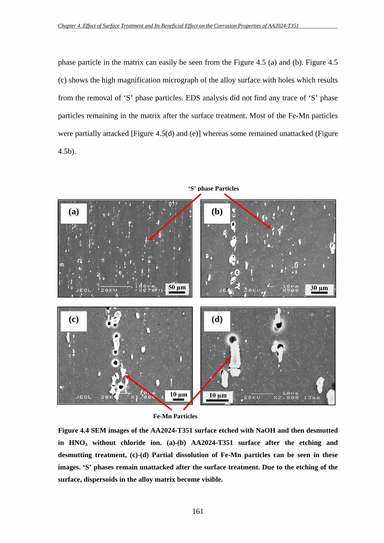
Chapter 4. Effect of Surface Treatment and Its Beneficial Effect on the Corrosion Properties of AA2024-T351
161
phase particle in the matrix can easily be seen from the Figure 4.5 (a) and (b). Figure 4.5
(c) shows the high magnification micrograph of the alloy surface with holes which results
from the removal of ‘S’ phase particles. EDS analysis did not find any trace of ‘S’ phase
particles remaining in the matrix after the surface treatment. Most of the Fe-Mn particles
were partially attacked [Figure 4.5(d) and (e)] whereas some remained unattacked (Figure
4.5b).
Figure 4.4 SEM images of the AA2024-T351 surface etched with NaOH and then desmutted
in HNO3 without chloride ion. (a)-(b) AA2024-T351 surface after the etching and
desmutting treatment, (c)-(d) Partial dissolution of Fe-Mn particles can be seen in these
images. ‘S’ phases remain unattacked after the surface treatment. Due to the etching of the
surface, dispersoids in the alloy matrix become visible.
(a) (b)
(c) (d)
‘S’ phase Particles
Fe-Mn Particles
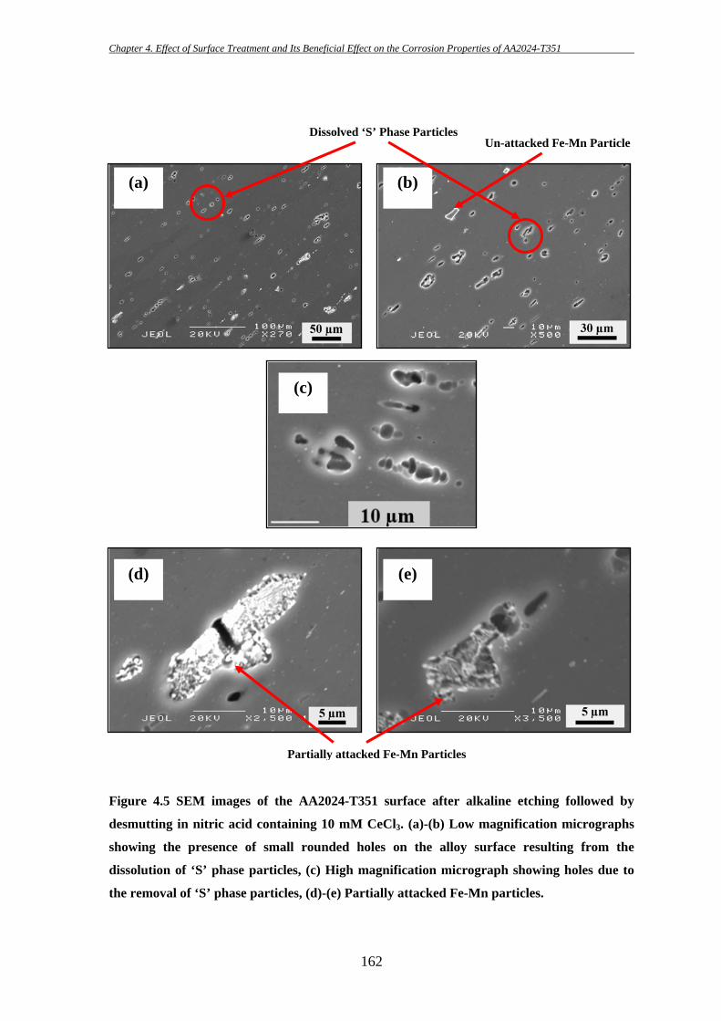
Chapter 4. Effect of Surface Treatment and Its Beneficial Effect on the Corrosion Properties of AA2024-T351
162
Figure 4.5 SEM images of the AA2024-T351 surface after alkaline etching followed by
desmutting in nitric acid containing 10 mM CeCl3. (a)-(b) Low magnification micrographs
showing the presence of small rounded holes on the alloy surface resulting from the
dissolution of ‘S’ phase particles, (c) High magnification micrograph showing holes due to
the removal of ‘S’ phase particles, (d)-(e) Partially attacked Fe-Mn particles.
(d) (e)
Partially attacked Fe-Mn Particles
(c)
(a) (b)
Dissolved ‘S’ Phase ParticlesUn-attacked Fe-Mn Particle
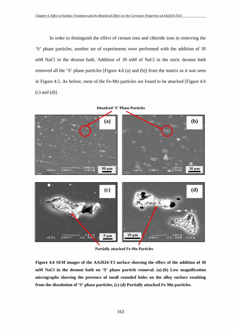
Chapter 4. Effect of Surface Treatment and Its Beneficial Effect on the Corrosion Properties of AA2024-T351
163
In order to distinguish the effect of cerium ions and chloride ions in removing the
‘S’ phase particles, another set of experiments were performed with the addition of 30
mM NaCl in the desmut bath. Addition of 30 mM of NaCl in the nitric desmut bath
removed all the ‘S’ phase particles [Figure 4.6 (a) and (b)] from the matrix as it was seen
in Figure 4.5. As before, most of the Fe-Mn particles are found to be attacked [Figure 4.6
(c) and (d)].
Figure 4.6 SEM images of the AA2024-T3 surface showing the effect of the addition of 30
mM NaCl in the desmut bath on ‘S’ phase particle removal. (a)-(b) Low magnification
micrographs showing the presence of small rounded holes on the alloy surface resulting
from the dissolution of ‘S’ phase particles, (c)-(d) Partially attacked Fe-Mn particles.
(a) (b)
Dissolved ‘S’ Phase Particles
(c) (d)
Partially attacked Fe-Mn Particles
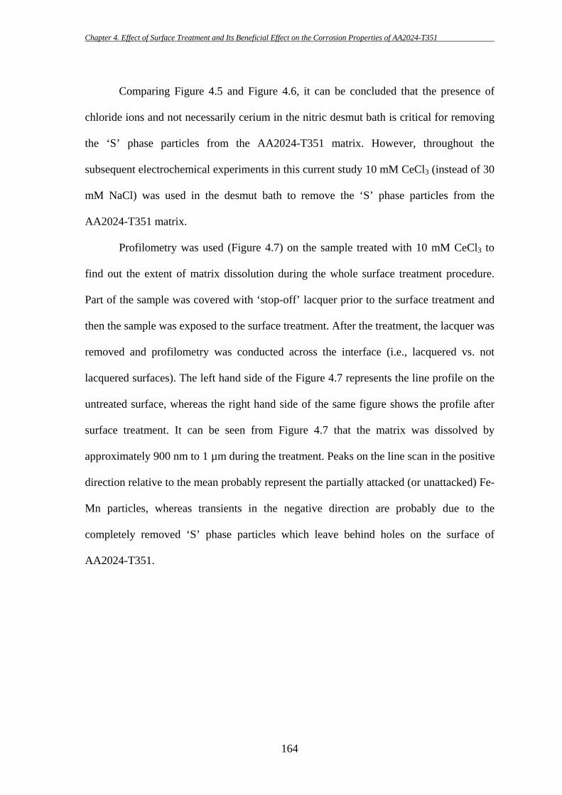
Chapter 4. Effect of Surface Treatment and Its Beneficial Effect on the Corrosion Properties of AA2024-T351
164
Comparing Figure 4.5 and Figure 4.6, it can be concluded that the presence of
chloride ions and not necessarily cerium in the nitric desmut bath is critical for removing
the ‘S’ phase particles from the AA2024-T351 matrix. However, throughout the
subsequent electrochemical experiments in this current study 10 mM CeCl3 (instead of 30
mM NaCl) was used in the desmut bath to remove the ‘S’ phase particles from the
AA2024-T351 matrix.
Profilometry was used (Figure 4.7) on the sample treated with 10 mM CeCl3 to
find out the extent of matrix dissolution during the whole surface treatment procedure.
Part of the sample was covered with ‘stop-off’ lacquer prior to the surface treatment and
then the sample was exposed to the surface treatment. After the treatment, the lacquer was
removed and profilometry was conducted across the interface (i.e., lacquered vs. not
lacquered surfaces). The left hand side of the Figure 4.7 represents the line profile on the
untreated surface, whereas the right hand side of the same figure shows the profile after
surface treatment. It can be seen from Figure 4.7 that the matrix was dissolved by
approximately 900 nm to 1 µm during the treatment. Peaks on the line scan in the positive
direction relative to the mean probably represent the partially attacked (or unattacked) Fe-
Mn particles, whereas transients in the negative direction are probably due to the
completely removed ‘S’ phase particles which leave behind holes on the surface of
AA2024-T351.
Chapter 4. Effect of Surface Treatment and Its Beneficial Effect on the Corrosion Properties of AA2024-T351
165
-1500
-1000
-500
0
500
0 500 1000 1500 2000
Hei
ght (
nm)
Distance (µm)
Untreated
Surface treated
~ 1 µm
Figure 4.7 Line profilometric study (using Stylet Profilometer DekTak® 6M) showing the
depth of attack during the surface treatment as measured between the untreated and
treated part of the same AA2024-T351 sample. Surface treatment resulted in almost one
micron depth of alloy dissolution.
4.3 Anodic Potentiodynamic Polarization Measurements
4.3.1 In Naturally Aerated 10 mM NaCl Solution
Anodic potentiodynamic polarization scans were performed in naturally aerated
10 mM NaCl solution at room temperature on as received and different surface treated
samples as shown in Figure 4.8. Scans were performed with a rate of 1 mV/s and on
freshly polished exposed sample area of 1.2 cm2 of one micron surface finish. Apart from
the etched and surface treated samples, scans were also performed on the samples only
dipped in HNO3 for 30s after polishing. These scans are represented with the blue colour.
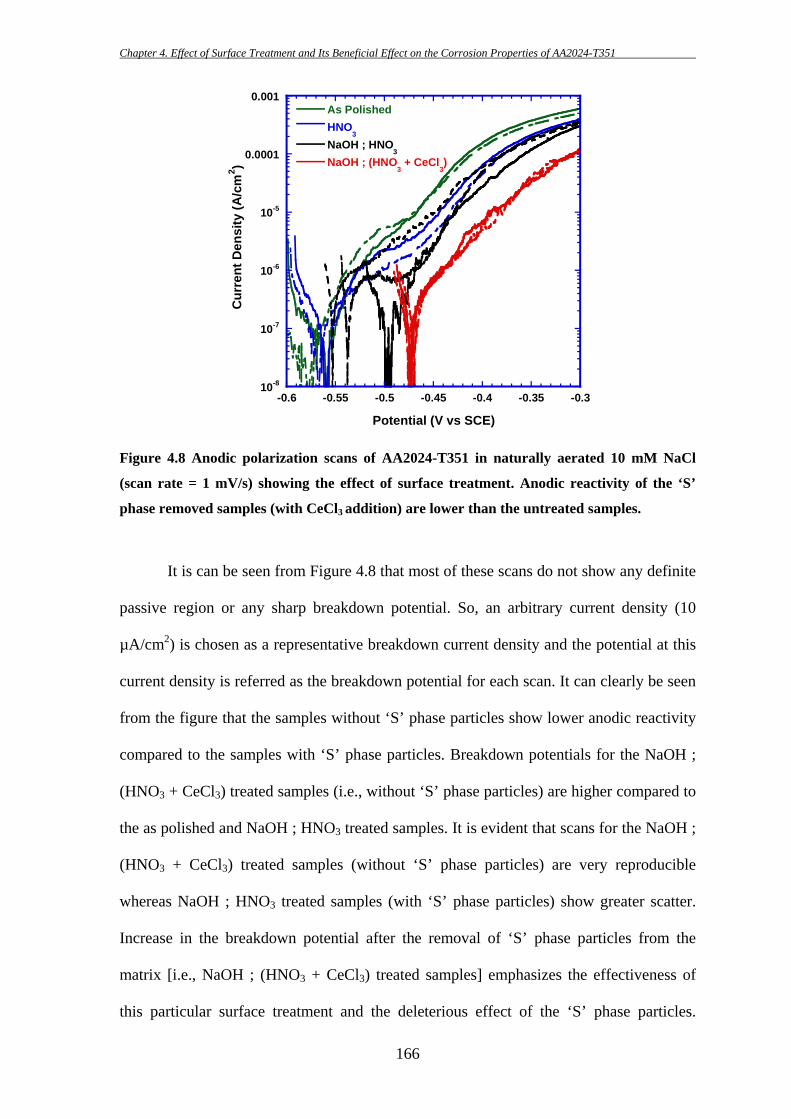
Chapter 4. Effect of Surface Treatment and Its Beneficial Effect on the Corrosion Properties of AA2024-T351
166
10-8
10-7
10-6
10-5
0.0001
0.001
-0.6 -0.55 -0.5 -0.45 -0.4 -0.35 -0.3
As PolishedHNO
3NaOH ; HNO
3NaOH ; (HNO
3 + CeCl
3)
Cur
rent
Den
sity
(A/c
m2 )
Potential (V vs SCE)
Figure 4.8 Anodic polarization scans of AA2024-T351 in naturally aerated 10 mM NaCl
(scan rate = 1 mV/s) showing the effect of surface treatment. Anodic reactivity of the ‘S’
phase removed samples (with CeCl3 addition) are lower than the untreated samples.
It is can be seen from Figure 4.8 that most of these scans do not show any definite
passive region or any sharp breakdown potential. So, an arbitrary current density (10
µA/cm2) is chosen as a representative breakdown current density and the potential at this
current density is referred as the breakdown potential for each scan. It can clearly be seen
from the figure that the samples without ‘S’ phase particles show lower anodic reactivity
compared to the samples with ‘S’ phase particles. Breakdown potentials for the NaOH ;
(HNO3 + CeCl3) treated samples (i.e., without ‘S’ phase particles) are higher compared to
the as polished and NaOH ; HNO3 treated samples. It is evident that scans for the NaOH ;
(HNO3 + CeCl3) treated samples (without ‘S’ phase particles) are very reproducible
whereas NaOH ; HNO3 treated samples (with ‘S’ phase particles) show greater scatter.
Increase in the breakdown potential after the removal of ‘S’ phase particles from the
matrix [i.e., NaOH ; (HNO3 + CeCl3) treated samples] emphasizes the effectiveness of
this particular surface treatment and the deleterious effect of the ‘S’ phase particles.
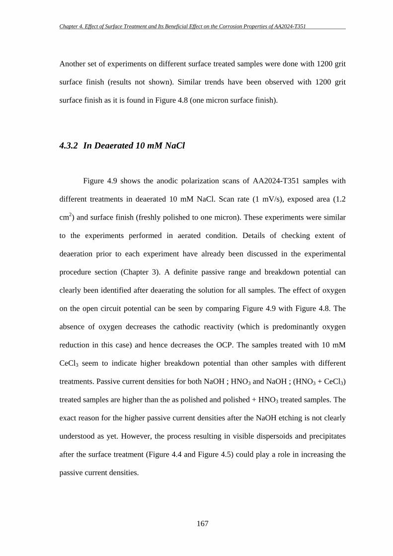
Chapter 4. Effect of Surface Treatment and Its Beneficial Effect on the Corrosion Properties of AA2024-T351
167
Another set of experiments on different surface treated samples were done with 1200 grit
surface finish (results not shown). Similar trends have been observed with 1200 grit
surface finish as it is found in Figure 4.8 (one micron surface finish).
4.3.2 In Deaerated 10 mM NaCl
Figure 4.9 shows the anodic polarization scans of AA2024-T351 samples with
different treatments in deaerated 10 mM NaCl. Scan rate (1 mV/s), exposed area (1.2
cm2) and surface finish (freshly polished to one micron). These experiments were similar
to the experiments performed in aerated condition. Details of checking extent of
deaeration prior to each experiment have already been discussed in the experimental
procedure section (Chapter 3). A definite passive range and breakdown potential can
clearly been identified after deaerating the solution for all samples. The effect of oxygen
on the open circuit potential can be seen by comparing Figure 4.9 with Figure 4.8. The
absence of oxygen decreases the cathodic reactivity (which is predominantly oxygen
reduction in this case) and hence decreases the OCP. The samples treated with 10 mM
CeCl3 seem to indicate higher breakdown potential than other samples with different
treatments. Passive current densities for both NaOH ; HNO3 and NaOH ; (HNO3 + CeCl3)
treated samples are higher than the as polished and polished + HNO3 treated samples. The
exact reason for the higher passive current densities after the NaOH etching is not clearly
understood as yet. However, the process resulting in visible dispersoids and precipitates
after the surface treatment (Figure 4.4 and Figure 4.5) could play a role in increasing the
passive current densities.
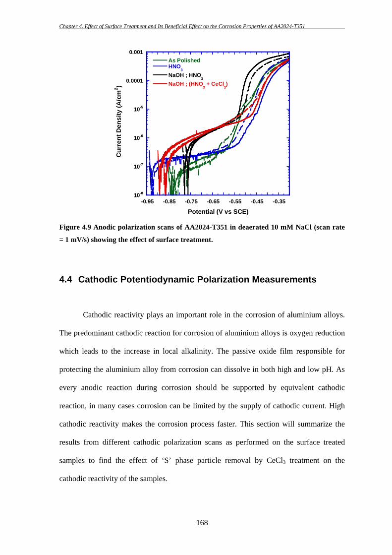
Chapter 4. Effect of Surface Treatment and Its Beneficial Effect on the Corrosion Properties of AA2024-T351
168
10-8
10-7
10-6
10-5
0.0001
0.001
-0.95 -0.85 -0.75 -0.65 -0.55 -0.45 -0.35
As PolishedHNO
3NaOH ; HNO
3
NaOH ; (HNO3 + CeCl
3)
Cur
rent
Den
sity
(A/c
m2 )
Potential (V vs SCE)
Figure 4.9 Anodic polarization scans of AA2024-T351 in deaerated 10 mM NaCl (scan rate
= 1 mV/s) showing the effect of surface treatment.
4.4 Cathodic Potentiodynamic Polarization Measurements
Cathodic reactivity plays an important role in the corrosion of aluminium alloys.
The predominant cathodic reaction for corrosion of aluminium alloys is oxygen reduction
which leads to the increase in local alkalinity. The passive oxide film responsible for
protecting the aluminium alloy from corrosion can dissolve in both high and low pH. As
every anodic reaction during corrosion should be supported by equivalent cathodic
reaction, in many cases corrosion can be limited by the supply of cathodic current. High
cathodic reactivity makes the corrosion process faster. This section will summarize the
results from different cathodic polarization scans as performed on the surface treated
samples to find the effect of ‘S’ phase particle removal by CeCl3 treatment on the
cathodic reactivity of the samples.
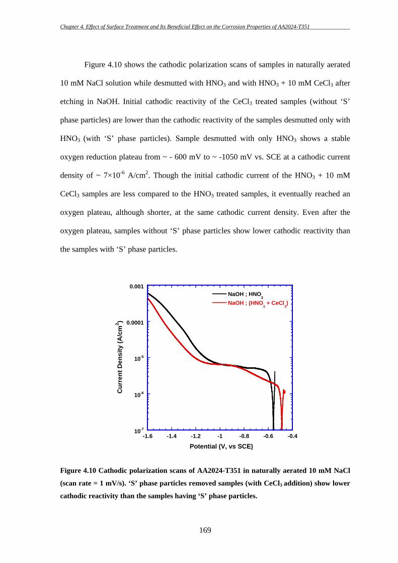
Chapter 4. Effect of Surface Treatment and Its Beneficial Effect on the Corrosion Properties of AA2024-T351
169
10-7
10-6
10-5
0.0001
0.001
-1.6 -1.4 -1.2 -1 -0.8 -0.6 -0.4
NaOH ; HNO3
NaOH ; (HNO3 + CeCl
3)
Cur
rent
Den
sity
(A/c
m2 )
Potential (V, vs SCE)
Figure 4.10 shows the cathodic polarization scans of samples in naturally aerated
10 mM NaCl solution while desmutted with HNO3 and with HNO3 + 10 mM CeCl3 after
etching in NaOH. Initial cathodic reactivity of the CeCl3 treated samples (without ‘S’
phase particles) are lower than the cathodic reactivity of the samples desmutted only with
HNO3 (with ‘S’ phase particles). Sample desmutted with only HNO3 shows a stable
oxygen reduction plateau from ~ - 600 mV to ~ -1050 mV vs. SCE at a cathodic current
density of ~ 7×10⁻⁶ A/cm2. Though the initial cathodic current of the HNO3 + 10 mM
CeCl3 samples are less compared to the HNO3 treated samples, it eventually reached an
oxygen plateau, although shorter, at the same cathodic current density. Even after the
oxygen plateau, samples without ‘S’ phase particles show lower cathodic reactivity than
the samples with ‘S’ phase particles.
Figure 4.10 Cathodic polarization scans of AA2024-T351 in naturally aerated 10 mM NaCl
(scan rate = 1 mV/s). ‘S’ phase particles removed samples (with CeCl3 addition) show lower
cathodic reactivity than the samples having ‘S’ phase particles.
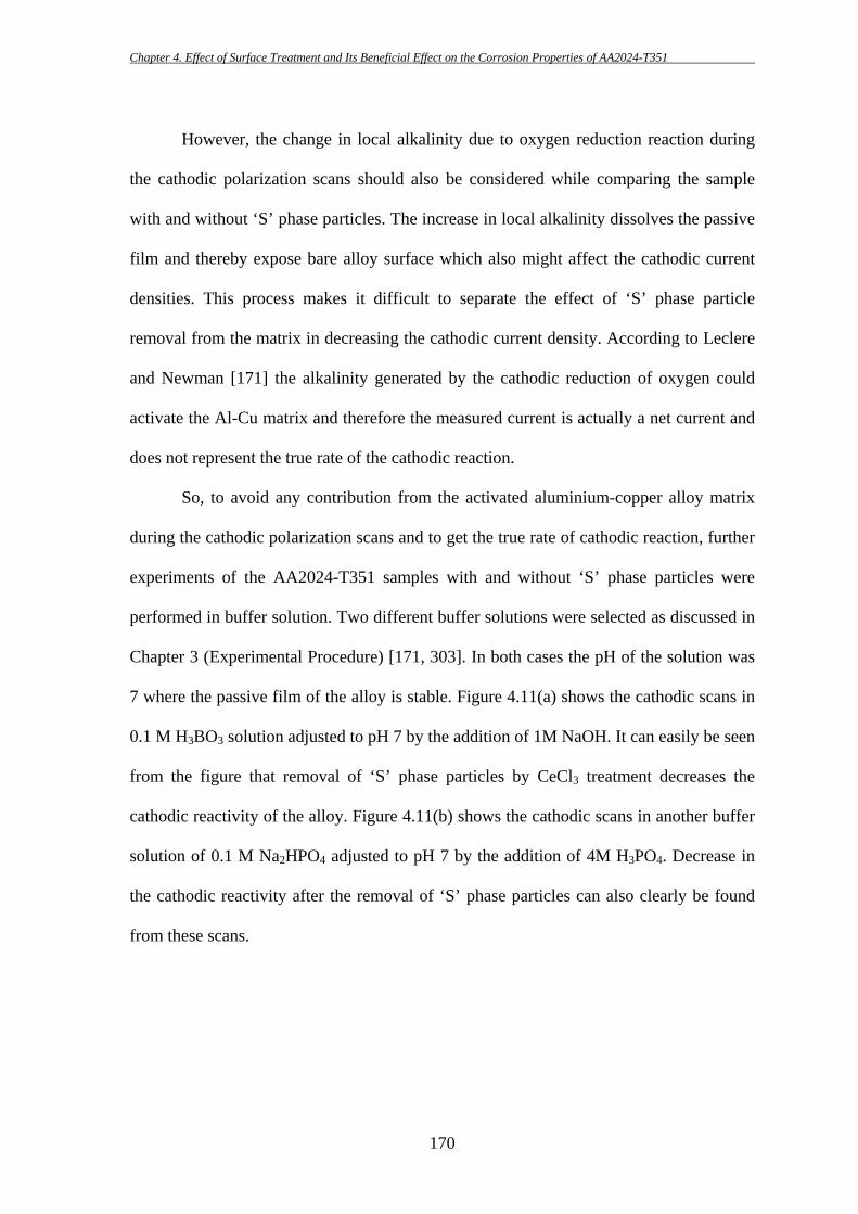
Chapter 4. Effect of Surface Treatment and Its Beneficial Effect on the Corrosion Properties of AA2024-T351
170
However, the change in local alkalinity due to oxygen reduction reaction during
the cathodic polarization scans should also be considered while comparing the sample
with and without ‘S’ phase particles. The increase in local alkalinity dissolves the passive
film and thereby expose bare alloy surface which also might affect the cathodic current
densities. This process makes it difficult to separate the effect of ‘S’ phase particle
removal from the matrix in decreasing the cathodic current density. According to Leclere
and Newman [171] the alkalinity generated by the cathodic reduction of oxygen could
activate the Al-Cu matrix and therefore the measured current is actually a net current and
does not represent the true rate of the cathodic reaction.
So, to avoid any contribution from the activated aluminium-copper alloy matrix
during the cathodic polarization scans and to get the true rate of cathodic reaction, further
experiments of the AA2024-T351 samples with and without ‘S’ phase particles were
performed in buffer solution. Two different buffer solutions were selected as discussed in
Chapter 3 (Experimental Procedure) [171, 303]. In both cases the pH of the solution was
7 where the passive film of the alloy is stable. Figure 4.11(a) shows the cathodic scans in
0.1 M H3BO3 solution adjusted to pH 7 by the addition of 1M NaOH. It can easily be seen
from the figure that removal of ‘S’ phase particles by CeCl3 treatment decreases the
cathodic reactivity of the alloy. Figure 4.11(b) shows the cathodic scans in another buffer
solution of 0.1 M Na2HPO4 adjusted to pH 7 by the addition of 4M H3PO4. Decrease in
the cathodic reactivity after the removal of ‘S’ phase particles can also clearly be found
from these scans.
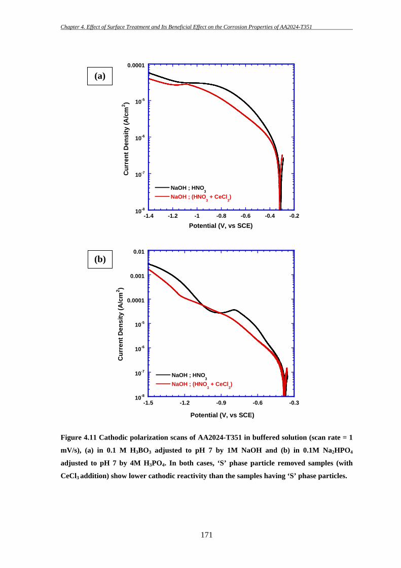
Chapter 4. Effect of Surface Treatment and Its Beneficial Effect on the Corrosion Properties of AA2024-T351
171
Figure 4.11 Cathodic polarization scans of AA2024-T351 in buffered solution (scan rate = 1
mV/s), (a) in 0.1 M H3BO3 adjusted to pH 7 by 1M NaOH and (b) in 0.1M Na2HPO4
adjusted to pH 7 by 4M H3PO4. In both cases, ‘S’ phase particle removed samples (with
CeCl3 addition) show lower cathodic reactivity than the samples having ‘S’ phase particles.
(a)
(b)
10-8
10-7
10-6
10-5
0.0001
-1.4 -1.2 -1 -0.8 -0.6 -0.4 -0.2
NaOH ; HNO3
NaOH ; (HNO3 + CeCl
3)
Cur
rent
Den
sity
(A/c
m2 )
Potential (V, vs SCE)
10-8
10-7
10-6
10-5
0.0001
0.001
0.01
-1.5 -1.2 -0.9 -0.6 -0.3
NaOH ; HNO3
NaOH ; (HNO3 + CeCl
3)
Cur
rent
Den
sity
(A/c
m2 )
Potential (V, vs SCE)
Chapter 4. Effect of Surface Treatment and Its Beneficial Effect on the Corrosion Properties of AA2024-T351
172
4.5 Open Circuit Potential (OCP) Measurements
4.5.1 Short Term OCP measurements
Short term OCP measurement of the AA2024-T351 samples desmutted with
HNO3 and with HNO3 + 10mM CeCl3 were performed in naturally aerated 10 mM NaCl
Figure 4.12. The main objective of this short term exposure is to capture the initial
potential fluctuations with high data collection frequency and to analyze the sample
surface with optical microscopy after the experiment. Samples exposed for short times
have less chance of generating a layer of corrosion products on the surface and so it is
possible to take micrographs of the attack morphologies.
Figure 4.12 shows the variations in the open circuit potentials as a function of
time for samples with ‘S’ phase particles (desmutted with HNO3) and without ‘S’ phase
particles (desmutted with HNO3 + 10 mM CeCl3). It can be seen from the figure that
samples desmutted with HNO3 have a lot of transients/fluctuations in the OCP, whereas
samples desmutted with HNO3 + 10 mM CeCl3 show very smooth OCP curve. The
transients/fluctuations in the OCP are thought to be correlated with the corrosion process
on the sample surface. Samples desmutted with HNO3 has shown few sudden drops in
potentials (e.g., at ~ 700 and ~ 950 s) which are indicative of pitting corrosion. HNO3 +
10 mM CeCl3 desmutted samples show lower open circuit potential initially, but after
about 400 s the OCP value starts to increase and becomes similar to that of the HNO3
desmutted samples (~ - 500 mV vs. SCE).
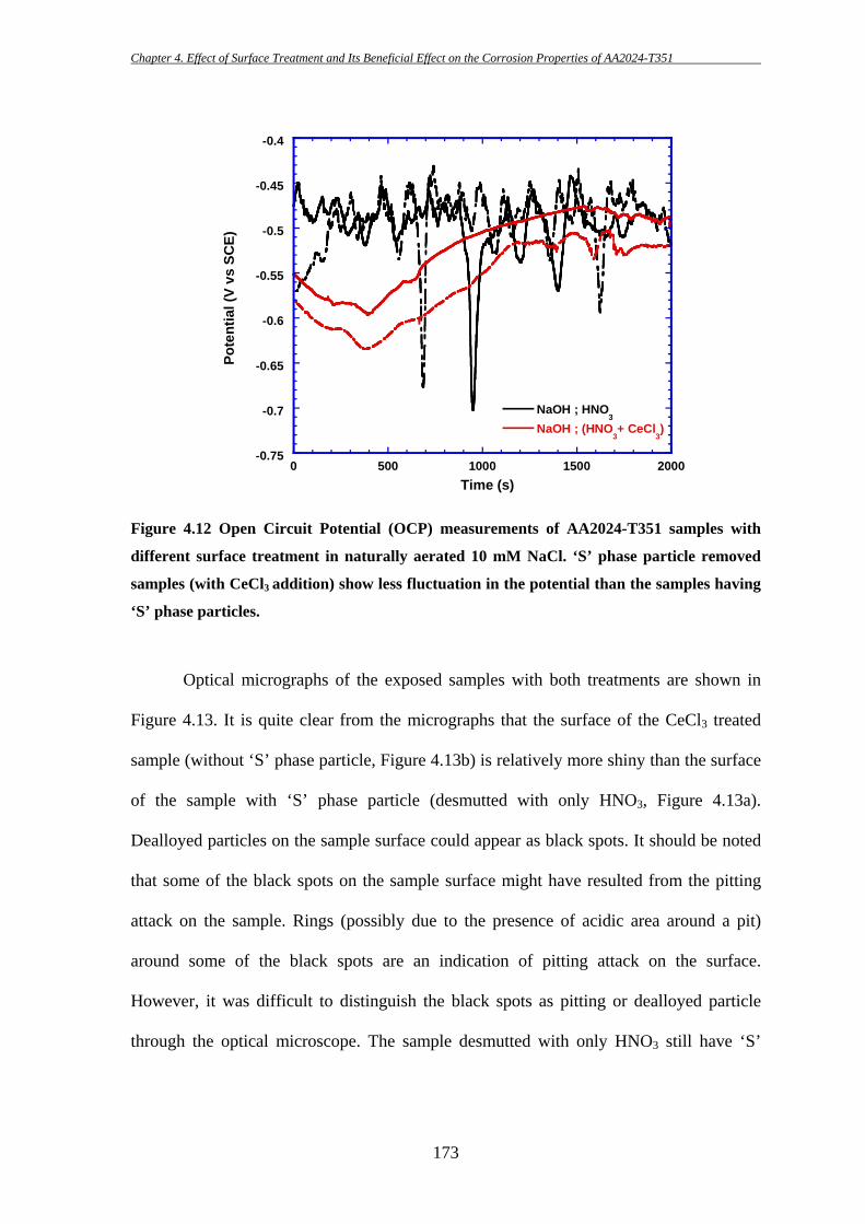
Chapter 4. Effect of Surface Treatment and Its Beneficial Effect on the Corrosion Properties of AA2024-T351
173
-0.75
-0.7
-0.65
-0.6
-0.55
-0.5
-0.45
-0.4
0 500 1000 1500 2000
NaOH ; HNO3
NaOH ; (HNO3+ CeCl
3)
Pote
ntia
l (V
vs S
CE)
Time (s)
Figure 4.12 Open Circuit Potential (OCP) measurements of AA2024-T351 samples with
different surface treatment in naturally aerated 10 mM NaCl. ‘S’ phase particle removed
samples (with CeCl3 addition) show less fluctuation in the potential than the samples having
‘S’ phase particles.
Optical micrographs of the exposed samples with both treatments are shown in
Figure 4.13. It is quite clear from the micrographs that the surface of the CeCl3 treated
sample (without ‘S’ phase particle, Figure 4.13b) is relatively more shiny than the surface
of the sample with ‘S’ phase particle (desmutted with only HNO3, Figure 4.13a).
Dealloyed particles on the sample surface could appear as black spots. It should be noted
that some of the black spots on the sample surface might have resulted from the pitting
attack on the sample. Rings (possibly due to the presence of acidic area around a pit)
around some of the black spots are an indication of pitting attack on the surface.
However, it was difficult to distinguish the black spots as pitting or dealloyed particle
through the optical microscope. The sample desmutted with only HNO3 still have ‘S’
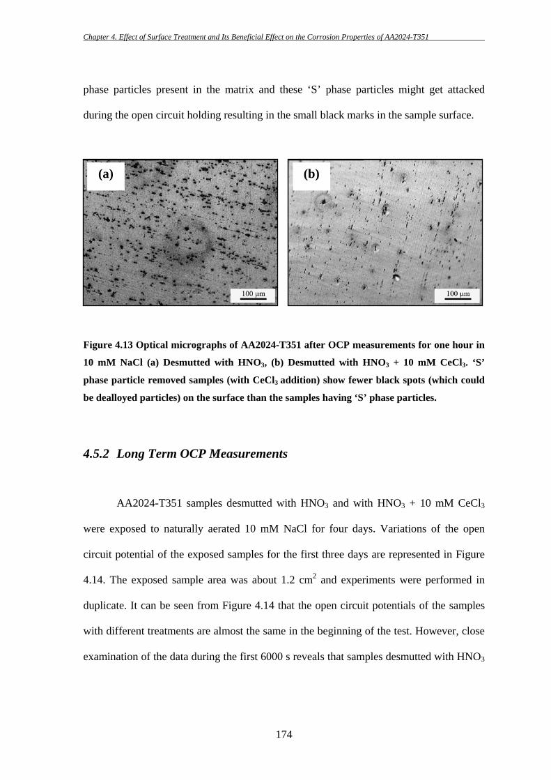
Chapter 4. Effect of Surface Treatment and Its Beneficial Effect on the Corrosion Properties of AA2024-T351
174
phase particles present in the matrix and these ‘S’ phase particles might get attacked
during the open circuit holding resulting in the small black marks in the sample surface.
Figure 4.13 Optical micrographs of AA2024-T351 after OCP measurements for one hour in
10 mM NaCl (a) Desmutted with HNO3, (b) Desmutted with HNO3 + 10 mM CeCl3. ‘S’
phase particle removed samples (with CeCl3 addition) show fewer black spots (which could
be dealloyed particles) on the surface than the samples having ‘S’ phase particles.
4.5.2 Long Term OCP Measurements
AA2024-T351 samples desmutted with HNO3 and with HNO3 + 10 mM CeCl3
were exposed to naturally aerated 10 mM NaCl for four days. Variations of the open
circuit potential of the exposed samples for the first three days are represented in Figure
4.14. The exposed sample area was about 1.2 cm2 and experiments were performed in
duplicate. It can be seen from Figure 4.14 that the open circuit potentials of the samples
with different treatments are almost the same in the beginning of the test. However, close
examination of the data during the first 6000 s reveals that samples desmutted with HNO3
(a) (b)
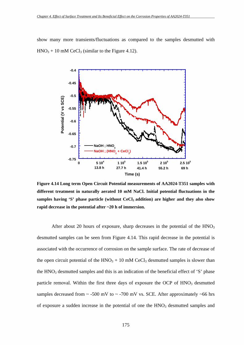
Chapter 4. Effect of Surface Treatment and Its Beneficial Effect on the Corrosion Properties of AA2024-T351
175
-0.75
-0.7
-0.65
-0.6
-0.55
-0.5
-0.45
-0.4
0 5 104 1 105 1.5 105 2 105 2.5 105
NaOH ; HNO3
NaOH ; (HNO3 + CeCl
3)
Pote
ntia
l (V
vs S
CE)
Time (s)13.8 h 27.7 h 41.4 h 55.2 h 69 h
show many more transients/fluctuations as compared to the samples desmutted with
HNO3 + 10 mM CeCl3 (similar to the Figure 4.12).
Figure 4.14 Long term Open Circuit Potential measurements of AA2024-T351 samples with
different treatment in naturally aerated 10 mM NaCl. Initial potential fluctuations in the
samples having ‘S’ phase particle (without CeCl3 addition) are higher and they also show
rapid decrease in the potential after ~20 h of immersion.
After about 20 hours of exposure, sharp decreases in the potential of the HNO3
desmutted samples can be seen from Figure 4.14. This rapid decrease in the potential is
associated with the occurrence of corrosion on the sample surface. The rate of decrease of
the open circuit potential of the HNO3 + 10 mM CeCl3 desmutted samples is slower than
the HNO3 desmutted samples and this is an indication of the beneficial effect of ‘S’ phase
particle removal. Within the first three days of exposure the OCP of HNO3 desmutted
samples decreased from ~ -500 mV to ~ -700 mV vs. SCE. After approximately ~66 hrs
of exposure a sudden increase in the potential of one the HNO3 desmutted samples and

Chapter 4. Effect of Surface Treatment and Its Beneficial Effect on the Corrosion Properties of AA2024-T351
176
gradual increase in one HNO3 + 10 mM CeCl3 desmutted samples can be observed. This
could probably be due to the formation of a scale of corrosion product on the corroding
surface.
After the test, the samples were found to be covered with white corrosion product.
Macrographs of the corroded samples are shown in Figure 4.15. Visual observations
showed some difference in sample appearance between the samples desmutted with
HNO3 and the samples desmutted with HNO3 + 10 mM CeCl3. Continuous corrosion
product cover can be seen on top of the HNO3 desmutted samples [Figure 4.15(a)]
whereas corrosion product seems to be discontinuous in some parts of the samples
desmutted with HNO3 + 10 mM CeCl3. It was attempted to remove the corrosion product
from the samples by cleaning with 70% (15.8 N) HNO3 [304]. However, the corrosion
product remained unattacked even after cleaning in HNO3 as it can be seen from Figure
4.15. Typical optical micrographs of the exposed samples after cleaning are shown in
Figure 4.16. Pitting could be observed on both types of samples as black spots on the
surface beneath the corrosion product layer. Ideally the cathodic regions should be
enriched with copper as a result of dealloying and should be seen as copper coloured
areas under the microscope. In contrast, the anodic regions are acidic in nature and are
expected to appear shiny in the microstructure.
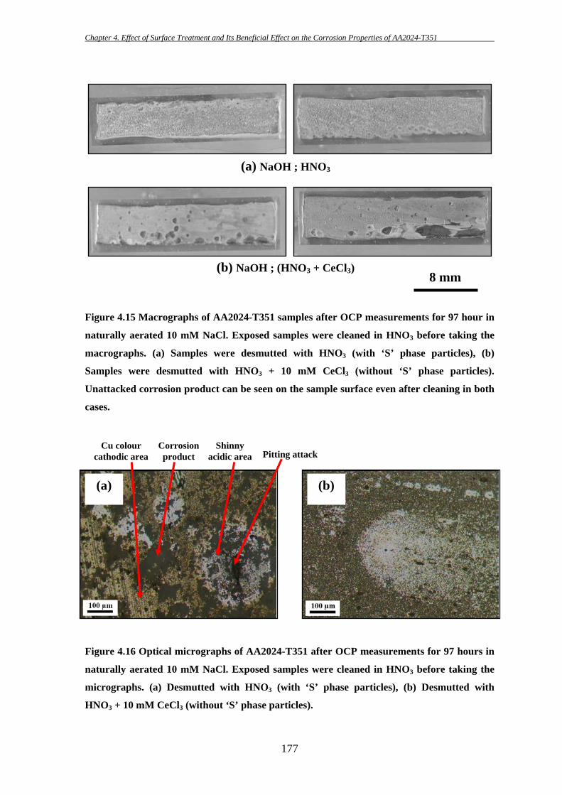
Chapter 4. Effect of Surface Treatment and Its Beneficial Effect on the Corrosion Properties of AA2024-T351
177
Figure 4.15 Macrographs of AA2024-T351 samples after OCP measurements for 97 hour in
naturally aerated 10 mM NaCl. Exposed samples were cleaned in HNO3 before taking the
macrographs. (a) Samples were desmutted with HNO3 (with ‘S’ phase particles), (b)
Samples were desmutted with HNO3 + 10 mM CeCl3 (without ‘S’ phase particles).
Unattacked corrosion product can be seen on the sample surface even after cleaning in both
cases.
Figure 4.16 Optical micrographs of AA2024-T351 after OCP measurements for 97 hours in
naturally aerated 10 mM NaCl. Exposed samples were cleaned in HNO3 before taking the
micrographs. (a) Desmutted with HNO3 (with ‘S’ phase particles), (b) Desmutted with
HNO3 + 10 mM CeCl3 (without ‘S’ phase particles).
8 mm
(a) NaOH ; HNO3
(b) NaOH ; (HNO3 + CeCl3)
(a) (b)
Pitting attack Shinny
acidic areaCu colour
cathodic area Corrosion product
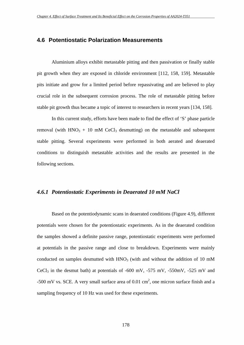
Chapter 4. Effect of Surface Treatment and Its Beneficial Effect on the Corrosion Properties of AA2024-T351
178
4.6 Potentiostatic Polarization Measurements
Aluminium alloys exhibit metastable pitting and then passivation or finally stable
pit growth when they are exposed in chloride environment [112, 158, 159]. Metastable
pits initiate and grow for a limited period before repassivating and are believed to play
crucial role in the subsequent corrosion process. The role of metastable pitting before
stable pit growth thus became a topic of interest to researchers in recent years [134, 158].
In this current study, efforts have been made to find the effect of ‘S’ phase particle
removal (with HNO3 + 10 mM CeCl3 desmutting) on the metastable and subsequent
stable pitting. Several experiments were performed in both aerated and deaerated
conditions to distinguish metastable activities and the results are presented in the
following sections.
4.6.1 Potentiostatic Experiments in Deaerated 10 mM NaCl
Based on the potentiodynamic scans in deaerated conditions (Figure 4.9), different
potentials were chosen for the potentiostatic experiments. As in the deaerated condition
the samples showed a definite passive range, potentiostatic experiments were performed
at potentials in the passive range and close to breakdown. Experiments were mainly
conducted on samples desmutted with HNO3 (with and without the addition of 10 mM
CeCl3 in the desmut bath) at potentials of -600 mV, -575 mV, -550mV, -525 mV and
-500 mV vs. SCE. A very small surface area of 0.01 cm2, one micron surface finish and a
sampling frequency of 10 Hz was used for these experiments.
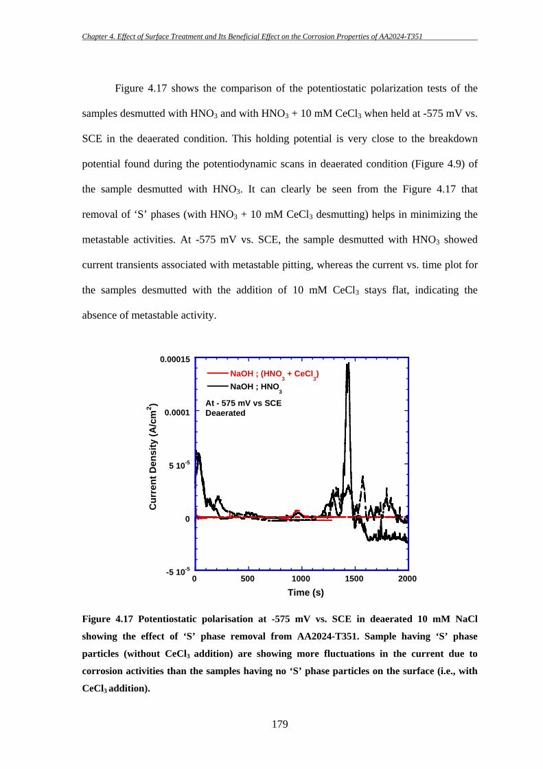
Chapter 4. Effect of Surface Treatment and Its Beneficial Effect on the Corrosion Properties of AA2024-T351
179
-5 10-5
0
5 10-5
0.0001
0.00015
0 500 1000 1500 2000
NaOH ; (HNO3 + CeCl
3)
NaOH ; HNO3
Cur
rent
Den
sity
(A/c
m2 )
Time (s)
At - 575 mV vs SCEDeaerated
Figure 4.17 shows the comparison of the potentiostatic polarization tests of the
samples desmutted with HNO3 and with HNO3 + 10 mM CeCl3 when held at -575 mV vs.
SCE in the deaerated condition. This holding potential is very close to the breakdown
potential found during the potentiodynamic scans in deaerated condition (Figure 4.9) of
the sample desmutted with HNO3. It can clearly be seen from the Figure 4.17 that
removal of ‘S’ phases (with HNO3 + 10 mM CeCl3 desmutting) helps in minimizing the
metastable activities. At -575 mV vs. SCE, the sample desmutted with HNO3 showed
current transients associated with metastable pitting, whereas the current vs. time plot for
the samples desmutted with the addition of 10 mM CeCl3 stays flat, indicating the
absence of metastable activity.
Figure 4.17 Potentiostatic polarisation at -575 mV vs. SCE in deaerated 10 mM NaCl
showing the effect of ‘S’ phase removal from AA2024-T351. Sample having ‘S’ phase
particles (without CeCl3 addition) are showing more fluctuations in the current due to
corrosion activities than the samples having no ‘S’ phase particles on the surface (i.e., with
CeCl3 addition).
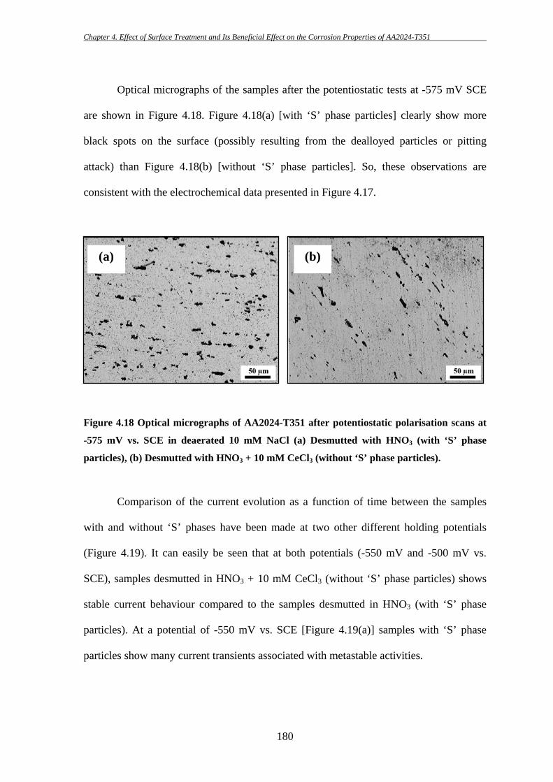
Chapter 4. Effect of Surface Treatment and Its Beneficial Effect on the Corrosion Properties of AA2024-T351
180
Optical micrographs of the samples after the potentiostatic tests at -575 mV SCE
are shown in Figure 4.18. Figure 4.18(a) [with ‘S’ phase particles] clearly show more
black spots on the surface (possibly resulting from the dealloyed particles or pitting
attack) than Figure 4.18(b) [without ‘S’ phase particles]. So, these observations are
consistent with the electrochemical data presented in Figure 4.17.
Figure 4.18 Optical micrographs of AA2024-T351 after potentiostatic polarisation scans at
-575 mV vs. SCE in deaerated 10 mM NaCl (a) Desmutted with HNO3 (with ‘S’ phase
particles), (b) Desmutted with HNO3 + 10 mM CeCl3 (without ‘S’ phase particles).
Comparison of the current evolution as a function of time between the samples
with and without ‘S’ phases have been made at two other different holding potentials
(Figure 4.19). It can easily be seen that at both potentials (-550 mV and -500 mV vs.
SCE), samples desmutted in HNO3 + 10 mM CeCl3 (without ‘S’ phase particles) shows
stable current behaviour compared to the samples desmutted in HNO3 (with ‘S’ phase
particles). At a potential of -550 mV vs. SCE [Figure 4.19(a)] samples with ‘S’ phase
particles show many current transients associated with metastable activities.
(a) (b)(a) (b)
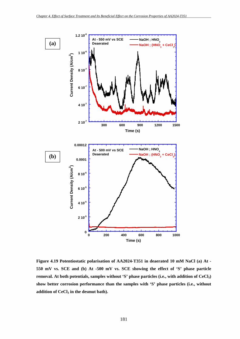
Chapter 4. Effect of Surface Treatment and Its Beneficial Effect on the Corrosion Properties of AA2024-T351
181
Figure 4.19 Potentiostatic polarisation of AA2024-T351 in deaerated 10 mM NaCl (a) At -
550 mV vs. SCE and (b) At -500 mV vs. SCE showing the effect of ‘S’ phase particle
removal. At both potentials, samples without ‘S’ phase particles (i.e., with addition of CeCl3)
show better corrosion performance than the samples with ‘S’ phase particles (i.e., without
addition of CeCl3 in the desmut bath).
(a)
(b)
2 10-7
4 10-7
6 10-7
8 10-7
1 10-6
1.2 10-6
300 600 900 1200 1500
NaOH ; HNO3
NaOH ; (HNO3 + CeCl
3)
Cur
rent
Den
sity
(A/c
m2 )
Time (s)
At - 550 mV vs SCEDeaerated
0
2 10-5
4 10-5
6 10-5
8 10-5
0.0001
0.00012
0 200 400 600 800 1000
NaOH ; HNO3
NaOH ; (HNO3 + CeCl
3)
Cur
rent
Den
sity
(A/c
m2 )
Time (s)
At - 500 mV vs SCEDeaerated
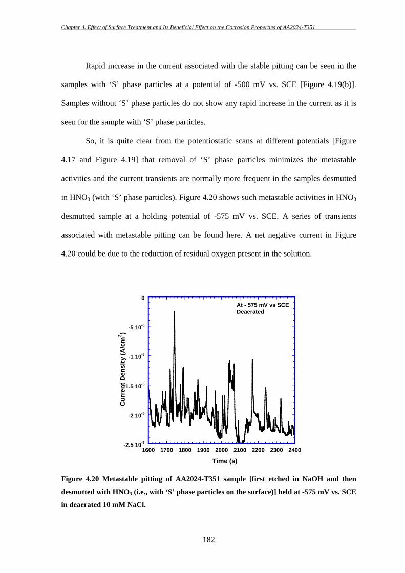
Chapter 4. Effect of Surface Treatment and Its Beneficial Effect on the Corrosion Properties of AA2024-T351
182
-2.5 10-5
-2 10-5
-1.5 10-5
-1 10-5
-5 10-6
0
1600 1700 1800 1900 2000 2100 2200 2300 2400
Time (s)
Cur
rent
Den
sity
(A/c
m2 )
At - 575 mV vs SCEDeaerated
Rapid increase in the current associated with the stable pitting can be seen in the
samples with ‘S’ phase particles at a potential of -500 mV vs. SCE [Figure 4.19(b)].
Samples without ‘S’ phase particles do not show any rapid increase in the current as it is
seen for the sample with ‘S’ phase particles.
So, it is quite clear from the potentiostatic scans at different potentials [Figure
4.17 and Figure 4.19] that removal of ‘S’ phase particles minimizes the metastable
activities and the current transients are normally more frequent in the samples desmutted
in HNO3 (with ‘S’ phase particles). Figure 4.20 shows such metastable activities in HNO3
desmutted sample at a holding potential of -575 mV vs. SCE. A series of transients
associated with metastable pitting can be found here. A net negative current in Figure
4.20 could be due to the reduction of residual oxygen present in the solution.
Figure 4.20 Metastable pitting of AA2024-T351 sample [first etched in NaOH and then
desmutted with HNO3 (i.e., with ‘S’ phase particles on the surface)] held at -575 mV vs. SCE
in deaerated 10 mM NaCl.
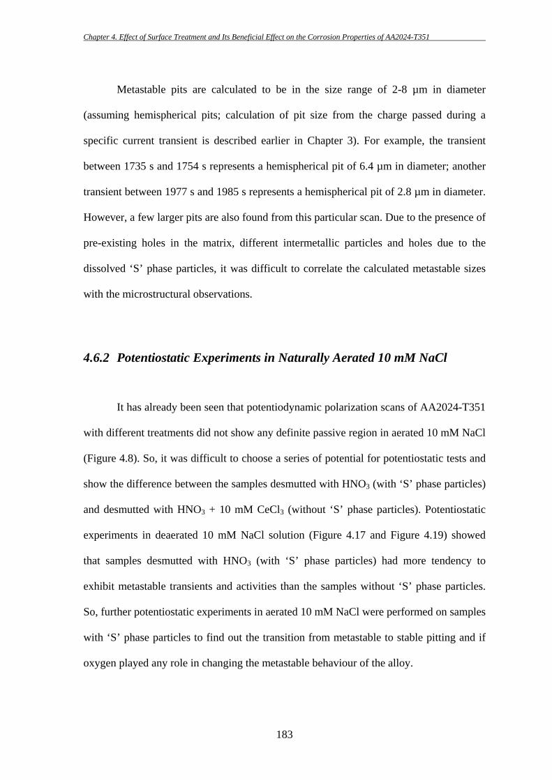
Chapter 4. Effect of Surface Treatment and Its Beneficial Effect on the Corrosion Properties of AA2024-T351
183
Metastable pits are calculated to be in the size range of 2-8 µm in diameter
(assuming hemispherical pits; calculation of pit size from the charge passed during a
specific current transient is described earlier in Chapter 3). For example, the transient
between 1735 s and 1754 s represents a hemispherical pit of 6.4 µm in diameter; another
transient between 1977 s and 1985 s represents a hemispherical pit of 2.8 µm in diameter.
However, a few larger pits are also found from this particular scan. Due to the presence of
pre-existing holes in the matrix, different intermetallic particles and holes due to the
dissolved ‘S’ phase particles, it was difficult to correlate the calculated metastable sizes
with the microstructural observations.
4.6.2 Potentiostatic Experiments in Naturally Aerated 10 mM NaCl
It has already been seen that potentiodynamic polarization scans of AA2024-T351
with different treatments did not show any definite passive region in aerated 10 mM NaCl
(Figure 4.8). So, it was difficult to choose a series of potential for potentiostatic tests and
show the difference between the samples desmutted with HNO3 (with ‘S’ phase particles)
and desmutted with HNO3 + 10 mM CeCl3 (without ‘S’ phase particles). Potentiostatic
experiments in deaerated 10 mM NaCl solution (Figure 4.17 and Figure 4.19) showed
that samples desmutted with HNO3 (with ‘S’ phase particles) had more tendency to
exhibit metastable transients and activities than the samples without ‘S’ phase particles.
So, further potentiostatic experiments in aerated 10 mM NaCl were performed on samples
with ‘S’ phase particles to find out the transition from metastable to stable pitting and if
oxygen played any role in changing the metastable behaviour of the alloy.
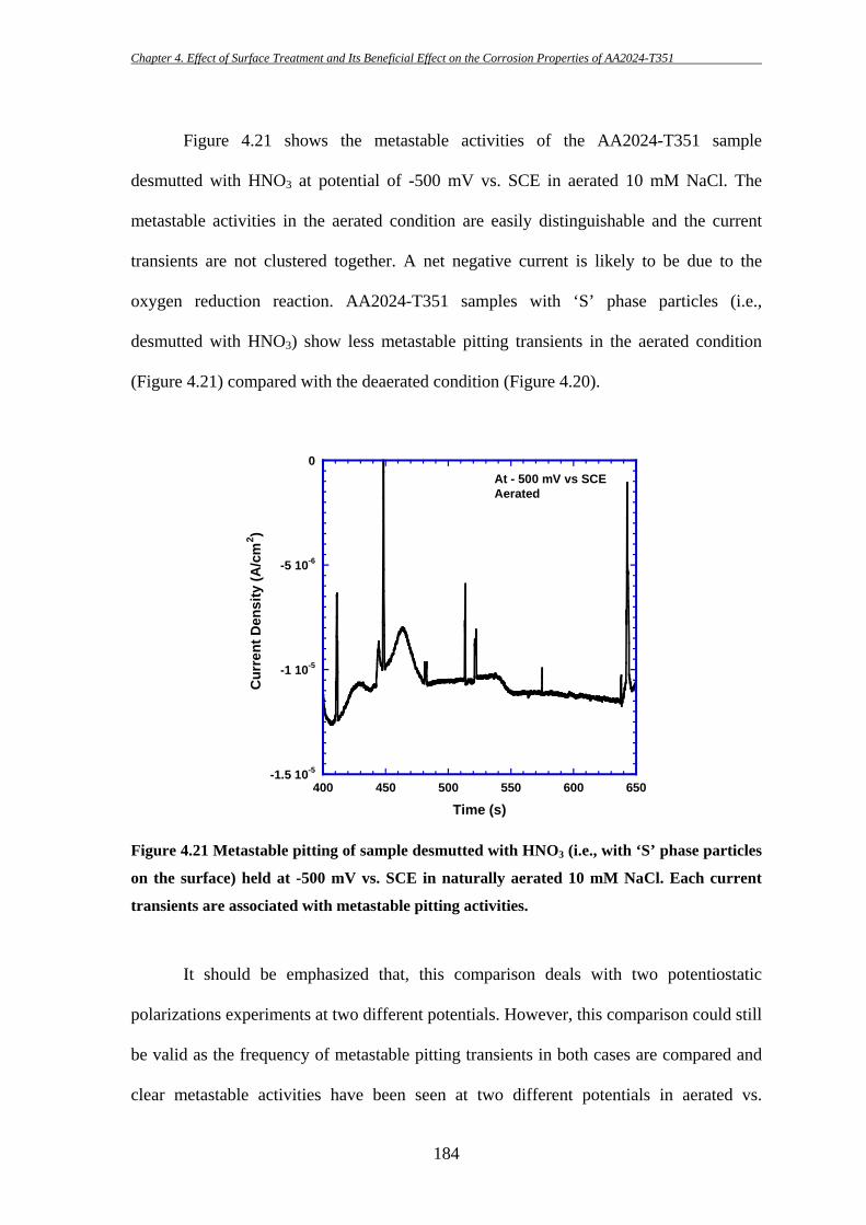
Chapter 4. Effect of Surface Treatment and Its Beneficial Effect on the Corrosion Properties of AA2024-T351
184
-1.5 10-5
-1 10-5
-5 10-6
0
400 450 500 550 600 650
Cur
rent
Den
sity
(A/c
m2 )
Time (s)
At - 500 mV vs SCEAerated
Figure 4.21 shows the metastable activities of the AA2024-T351 sample
desmutted with HNO3 at potential of -500 mV vs. SCE in aerated 10 mM NaCl. The
metastable activities in the aerated condition are easily distinguishable and the current
transients are not clustered together. A net negative current is likely to be due to the
oxygen reduction reaction. AA2024-T351 samples with ‘S’ phase particles (i.e.,
desmutted with HNO3) show less metastable pitting transients in the aerated condition
(Figure 4.21) compared with the deaerated condition (Figure 4.20).
Figure 4.21 Metastable pitting of sample desmutted with HNO3 (i.e., with ‘S’ phase particles
on the surface) held at -500 mV vs. SCE in naturally aerated 10 mM NaCl. Each current
transients are associated with metastable pitting activities.
It should be emphasized that, this comparison deals with two potentiostatic
polarizations experiments at two different potentials. However, this comparison could still
be valid as the frequency of metastable pitting transients in both cases are compared and
clear metastable activities have been seen at two different potentials in aerated vs.

Chapter 4. Effect of Surface Treatment and Its Beneficial Effect on the Corrosion Properties of AA2024-T351
185
-1.2 10-7
-1 10-7
-8 10-8
-6 10-8
-4 10-8
-2 10-8
0
2 10-8
445 446 447 448 449 450 451 452 453
Cur
rent
(A)
Time (s)
I peak
I OX
ti t
maxtf
At - 500 mV vs SCEAerated
deaerated solution (i.e., -575 mV vs. SCE for deaerated condition and -500 mV vs. SCE
for aerated condition). Metastable activities in the aerated condition are less even at a
higher potential (i.e., at -500 vs. SCE) as compared with the deaerated condition (i.e., at
-575 vs. SCE).
Figure 4.22 shows the shape of a typical metastable pit current peak. A rapid
increase in the current (at time ti) occurs on the onset of metastable pitting and at tmax the
peak current Ipeak is reached. The metastable pit can not sustain its growth, so
repassivation starts at tmax and finish at tf where the current return to its base value (i.e.,
passive current Iox). Based on the charge passed from time ti to tf (in Figure 4.22), the
diameter of the metastable pit is calculated to be about 2.3 µm.
Figure 4.22 Analysis of a single metastable pit of the AA2024-T351 sample desmutted with
HNO3 (i.e., with ‘S’ phase particles on the surface) held at -500 mV vs. SCE in naturally
aerated 10 mM NaCl. Total charge under such current transients can be calculated to find
out the metastable pit size assuming hemispherical pit geometry.

Chapter 4. Effect of Surface Treatment and Its Beneficial Effect on the Corrosion Properties of AA2024-T351
186
Several other metastable pit sizes are also calculated from Figure 4.21. Metastable
pit diameter between 410.2 s (ti) and 411.9 s (tf) is calculated to be approximately 2 µm.
Analysis showed that in deaerated solution metastable pits were approximately 2-8 µm in
diameter, whereas aerated experiments results in metastable pits of 1-4 µm in diameter.
These results on the alloy 2024-T351 are consistent with the findings of Pride et al. [134,
167] who reported metastable pitting in the same size range.
4.6.3 Role of Oxygen in Metastable Pitting
Comparison of the potentiostatic polarization scans in the deaerated and aerated
conditions as described in the earlier sections suggest that oxygen might play an
important role in the metastable pitting activities. The presence of oxygen in the system
seems to reduce the frequency of metastable pitting transients (comparison between
Figure 4.20 and Figure 4.21). The role of oxygen in reducing metastable activities is
clearly established in Figure 4.23 which shows the comparison of the potentiostatic tests
of AA2024-T351 samples desmutted in HNO3 in deaerated and aerated 10 mM NaCl at a
holding potential of -575 mV vs. SCE.
The initial increase in the current in both deaerated and aerated condition is
associated with the initiation of the localized attack. However, the subsequent decrease in
the current indicates that the localized attack does not propagate further. It is quite clear
from Figure 4.23 that metastable activities in the deaerated condition are more prominent
than in the aerated condition. After the initial decay, the current stays flat in the aerated
condition, whereas significant amount of current transients associated with metastable
pitting can be seen in the deaerated condition.
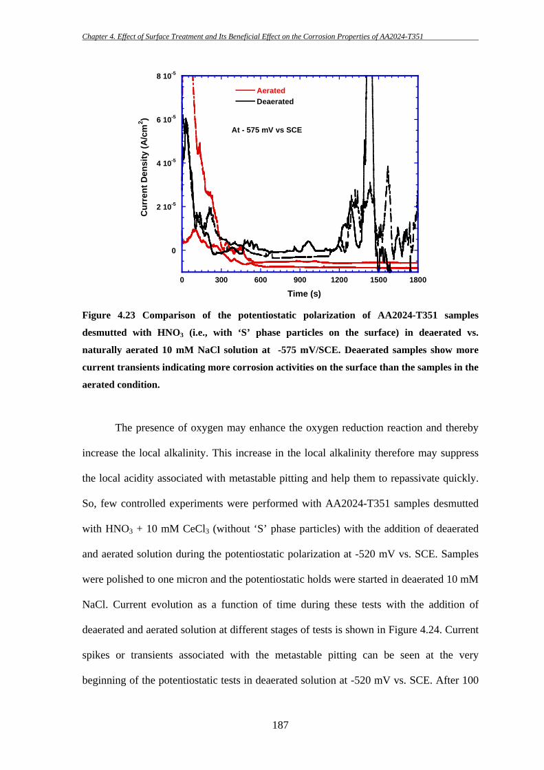
Chapter 4. Effect of Surface Treatment and Its Beneficial Effect on the Corrosion Properties of AA2024-T351
187
0
2 10-5
4 10-5
6 10-5
8 10-5
0 300 600 900 1200 1500 1800
AeratedDeaerated
At - 575 mV vs SCE
Cur
rent
Den
sity
(A/c
m2 )
Time (s)
Figure 4.23 Comparison of the potentiostatic polarization of AA2024-T351 samples
desmutted with HNO3 (i.e., with ‘S’ phase particles on the surface) in deaerated vs.
naturally aerated 10 mM NaCl solution at -575 mV/SCE. Deaerated samples show more
current transients indicating more corrosion activities on the surface than the samples in the
aerated condition.
The presence of oxygen may enhance the oxygen reduction reaction and thereby
increase the local alkalinity. This increase in the local alkalinity therefore may suppress
the local acidity associated with metastable pitting and help them to repassivate quickly.
So, few controlled experiments were performed with AA2024-T351 samples desmutted
with HNO3 + 10 mM CeCl3 (without ‘S’ phase particles) with the addition of deaerated
and aerated solution during the potentiostatic polarization at -520 mV vs. SCE. Samples
were polished to one micron and the potentiostatic holds were started in deaerated 10 mM
NaCl. Current evolution as a function of time during these tests with the addition of
deaerated and aerated solution at different stages of tests is shown in Figure 4.24. Current
spikes or transients associated with the metastable pitting can be seen at the very
beginning of the potentiostatic tests in deaerated solution at -520 mV vs. SCE. After 100
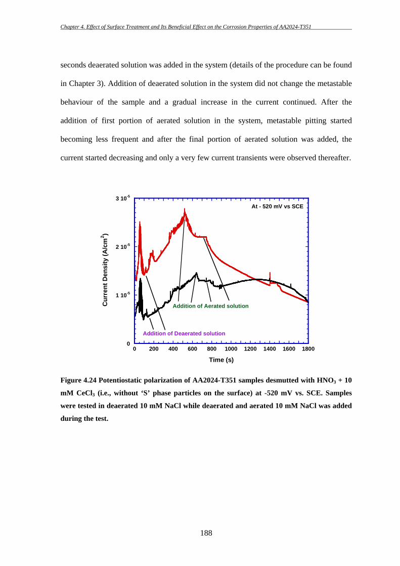
Chapter 4. Effect of Surface Treatment and Its Beneficial Effect on the Corrosion Properties of AA2024-T351
188
0
1 10-5
2 10-5
3 10-5
0 200 400 600 800 1000 1200 1400 1600 1800
Cur
rent
Den
sity
(A/c
m2 )
Time (s)
Addition of Deaerated solution
Addition of Aerated solution
At - 520 mV vs SCE
seconds deaerated solution was added in the system (details of the procedure can be found
in Chapter 3). Addition of deaerated solution in the system did not change the metastable
behaviour of the sample and a gradual increase in the current continued. After the
addition of first portion of aerated solution in the system, metastable pitting started
becoming less frequent and after the final portion of aerated solution was added, the
current started decreasing and only a very few current transients were observed thereafter.
Figure 4.24 Potentiostatic polarization of AA2024-T351 samples desmutted with HNO3 + 10
mM CeCl3 (i.e., without ‘S’ phase particles on the surface) at -520 mV vs. SCE. Samples
were tested in deaerated 10 mM NaCl while deaerated and aerated 10 mM NaCl was added
during the test.
Chapter 4. Effect of Surface Treatment and Its Beneficial Effect on the Corrosion Properties of AA2024-T351
189
4.7 Discussion
In this current study, two predominant categories of constituent intermetallics
particles have been identified in AA2024-T351 (Section 4.1). The first type is irregular in
shape and in the size range of 10-30 µm containing mainly Al-Cu-Fe-Mn (mentioned as
“Fe-Mn” particle throughout the study). Several other researchers [9, 11, 45, 56, 57, 72-
77, 204] have also documented presence of such type of coarse intermetallic particles in
AA2024 and therefore findings from the current study is consistent with those reported
earlier. In many cases, Fe-containing intermetallic particles are broken down in fragments
during subsequent thermo-mechanical treatment as seen in Figure 4.1(b) [7, 8, 81]. The
Fe-containing intermetallic particles from this present study seem to follow a
stoichiometric relationship close to Al15Cu3(Fe,Mn) [Table 4.1]. Very few Fe-containing
intermetallic particles in this current study have been found to have Si in it.
However, it should be noted that different batches of AA2024-T3 can have
different Si content and as a result some of the alloys reported in the literature show Fe-
rich intermetallic particles with Si and some other do not. For example, Chen et al. [8]
and Buchheit et al. [9] did not report the presence of Fe-rich intermetallic particle with Si
in AA2024-T3, whereas Campestrini [6] found Si containing Fe-rich intermetallic
particles in their study. Buchheit et al. [9] found that the ratio of Al to the sum of Cu, Fe,
and Mn was regularly 6 to 1 on an atomic percentage basis during their EDS analysis.
The average Cu:Fe:Mn ratio was 2:1:1 and varied little from particle to particle. Hence
they assigned the second largest category of Al-Cu-Fe-Mn particles to be chemically the
Al6(Cu,Fe,Mn) type. However, this current study emphasizes the fact as pointed out by
other researchers [7, 75] that the Fe-containing intermetallic particles may not possess
any definite stoichiometric relationship. Therefore, Fe-rich intermetallic particles in this
Chapter 4. Effect of Surface Treatment and Its Beneficial Effect on the Corrosion Properties of AA2024-T351
190
current study are referred as Fe-Mn phase/particles. Some of the Fe-Mn particles contain
more copper than the others as it is indicated by the relatively high standard deviation in
the copper content (Table 4.1 and Figure 4.3).
The second type of coarse intermetallic/constituent particle appeared as round and
smooth with a size range of 1-5 µm and were identified as Al2CuMg (‘S’ phase). The
number of ‘S’ phase particles in the matrix of AA2024-T351 are much higher that the Fe-
Mn particles. These findings are consistent with the literature as reported by several
researchers [5-9, 11, 19, 43-45, 70, 76, 80, 174, 198, 204, 211, 315]. In a few occasions
‘S’ phase particles are found to be in an elongated shape and as large as ~10 µm in size. A
small number of rounded and smooth particles are seen to contain Al and Cu. EDS
analysis show that stoichiometric of the Al-Cu particles are very close to Al2Cu and
therefore consistent with the findings of other researchers [75]. These Al2Cu particles are
small, rounded (1-2 µm) and generally found as isolated individual particles.
Intermetallic particles like ‘S’ phase particles and Fe-Mn particles play a crucial
role in determining the corrosion behaviour of AA2024-T351. Several researchers have
shown that pitting corrosion in aluminium alloys is normally associated with the
intermetallic particles [8-11, 14, 37, 38, 40, 42, 47, 48, 82, 123, 171, 173, 175, 181-197].
It is believed that Fe-Mn intermetallic particles generally act as cathode during the
corrosion process. Fe-Mn particles do not show selective dissolution, though pitting
sometime occurs at their periphery [7, 8, 11, 175, 186, 187]. In contrast, a number of
researchers have confirmed the anodic behaviour of ‘S’ phase particles by showing the
initiations of pits on the particles [8, 12, 37, 43, 46, 174, 185, 198]. It has to be mentioned
that, though the ‘S’ phase particles show initial anodic behaviour, they can then become
cathodically active because of dealloying and subsequent copper enrichment.
Chapter 4. Effect of Surface Treatment and Its Beneficial Effect on the Corrosion Properties of AA2024-T351
191
Electrochemical behaviour of each type of intermetallic particles will be discussed in
details in Chapter 5.
In order to find a suitable replacement for the chromate conversion coating as a
pretreatment technique, much focus has been given in the surface preparation of the
substrate by etching out the intermetallic particles (mostly cathodic in nature) from the
surface of the aluminium alloy. The fact that the chromate conversion coating is widely
used as a pretreatment technique because of its ability of inhibiting the cathodic oxygen
reduction reaction on the intermetallic particles and thereby minimising corrosion [74,
249, 250], researchers have tried to maintain this advantage (i.e., improved corrosion
properties and effectiveness in inhibiting the cathodic reaction) in the alternate
pretreatment methods [see Section 2.3 of Chapter 2 for more details]. Hence, one of the
main objectives of this chapter is to demonstrate an effective surface treatment technique
for removing deleterious ‘S’ phase particles from the surface of AA2024-T351 and to
investigate if the removal of ‘S’ phase particles can actually improve the corrosion
resistance of the alloy.
The effect of surface treatment on the appearance of different intermetallic
particles is shown in Section 4.2. It is found that addition of 10 mM CeCl3 in the nitric
acid desmut bath (after alkaline etching) completely removes the ‘S’ phase particles from
the surface of AA2024-T351 and partially attacks the Fe-Mn particles (Figure 4.5).
Desmutting only in a nitric acid bath (after alkaline etching) does not remove the ‘S’
phases from the matrix (Figure 4.4) although a few Fe-Mn particles are seen to be
attacked. Etching in sodium hydroxide does not remove the intermetallic particles
because in the alkaline environment Mg is stable and protects the ‘S’ phase particles.
These findings are also consistent with other researchers [19, 260] who found that
addition of rare earth chloride in the nitric acid bath helped in removing ‘S’ phase
Chapter 4. Effect of Surface Treatment and Its Beneficial Effect on the Corrosion Properties of AA2024-T351
192
intermetallic particles. However, the exact mechanism behind the ‘S’ phase particle
removal by the addition of CeCl3 in the desmut bath is not completely understood as yet.
Moulinier [19] showed that Cl- ions are actually responsible for removing the ‘S’ phase
particles, not the Ce3+ ions. In her study, addition of 30 mM NaCl showed similar effect
to that of the 10 mM CeCl3 addition in the desmut bath. But when 10 mM Ce(NO3)3 was
added to the desmut bath, ‘S’ phase remained unattacked. Addition of 30 mM NaCl in the
desmut bath in this current study has also shown a similar effect like 10 mM CeCl3
addition. So, it has clearly been established that Cl- ions are the actual responsible species
for removing ‘S’ phase particles.
During etching in NaOH, aluminium dissolves by forming aluminate ions,
Al(OH)4 and copper accumulates on the surface as a black deposit. Copper can react with
NaOH to form CuO which is a black oxide [see Section 2.3 for more details]. Matrix
dissolution during the surface treatment procedure is found to be approximately 900nm to
1µm (Figure 4.7). This value is consistent with the findings of others [19] with similar
surface treatments. Dissolution of the matrix mainly occurs during the etching process in
NaOH and additions of Cl- ions in the nitric acid desmut bath do not affect the extent of
matrix dissolution [19].
A series of anodic potentiodynamic polarization scans in both naturally aerated
and deaerated conditions show the beneficial effect of the surface treatment (i.e., ‘S’
phase particle removal) on the AA2024-T351 surface. In aerated condition (Figure 4.8),
samples without ‘S’ phase particles show lower anodic reactivity (and subsequent higher
breakdown potential) than the samples with ‘S’ phase particles. Beneficial effect of the
‘S’ phase particle removal by surface treatment can also be seen in the deaerated
condition (Figure 4.9) where samples without ‘S’ phase particles (i.e., with addition of
CeCl3 in the desmut bath) show higher breakdown potential than the samples with ‘S’
Chapter 4. Effect of Surface Treatment and Its Beneficial Effect on the Corrosion Properties of AA2024-T351
193
phase particles on the surface. Interestingly, the passive current density increases after the
samples are etched with sodium hydroxide. The exact reason for the higher passive
current densities after the NaOH etching is not clearly understood as yet. However, the
process resulting in visible dispersoids and precipitates after the surface treatment (Figure
4.4 and Figure 4.5) could play a role in increasing the passive current densities.
So, the improvement in the corrosion properties of AA2024-T351 after the ‘S’
phase particles removal in both aerated and deaerated condition establishes the
deleterious effect of ‘S’ phase particles in the corrosion initiation. These findings are
consistent with the researchers who identified ‘S’ phase particles as the most active phase
in AA2024-T351 and referred as the key contributor for the poor corrosion resistance of
AA2024-T351 [8, 9, 12, 37, 43, 46, 174, 185, 198] (further details about the corrosion
performances of ‘S’ phase particles and their role in pit initiation have already been
discussed in Section 2.2.1.2.1 of Chapter 2). Corrosion properties of these individual
intermetallic phases using microcapillary electrochemical cell (micro-cell) technique will
be discussed in details in Chapter 5. Initiation of localized corrosion in AA2024-T351 is
found in the form of pitting in all cases after the potentiodynamic scans.
Localized corrosion susceptibility of AA2024-T351 could be significantly
affected by the enhanced cathodic reactivity of the exposed area [70]. Addition of CeCl3
in the desmut bath not only enhances the dissolution of copper rich intermetallic particles
(i.e., ‘S’ phase particles) but also enhances the anodic dissolution of the copper
accumulated on the surface after etching [19]. ‘S’ phase particle initially behaves
anodically which results in the dealloying of Mg (and Al) from the particle. The particle
will soon become rich in Cu and start acting as cathode, as Cu is a better surface for
oxygen reduction. In several papers, Buchheit et al. [9, 14, 82, 123, 181, 182] described
the phenomena of Cu distribution in the surface during the corrosion process. So,
Chapter 4. Effect of Surface Treatment and Its Beneficial Effect on the Corrosion Properties of AA2024-T351
194
according to these observations and theories, addition of CeCl3 in the desmut bath should
result into the decrease in the cathodic reactivity of the AA2024-T351 as it removes the
‘S’ phase particles from the microstructure. Findings in this current study are consistent
with the proposed theories of other researchers as the addition of 10 mM CeCl3 in the
desmut bath reduce the cathodic reactivity of the AA2024-T351 sample (Figure 4.10).
Decrease in the cathodic reactivity after the removal of ‘S’ phase particles in this
current study is confirmed after the cathodic polarization scans in two different buffer
solutions (Figure 4.11). As discussed earlier, the increase in local alkalinity due to the
oxygen reduction reaction dissolves the passive film and exposes bare alloy surface which
also might affect the cathodic current densities. The use of buffer solution suppresses the
possibility of local alkalinity change and hence represent the true rate of the cathodic
reaction [171].
Open circuit potential (OCP, also referred as corrosion potential) measurements of
the surface treated AA2024-T351 samples without and with addition of 10 mM CeCl3 in
the desmut bath also proves the beneficial effects of ‘S’ phase particle removal from the
surface. Samples with ‘S’ phase particles (i.e., without addition of CeCl3) show more
fluctuations in the corrosion potential resulting from the corrosion activities (metastable
and stable pitting) on the surface (Figure 4.12 and Figure 4.13).
In chloride environments aluminium alloys exhibit metastable pitting and then
passivation or finally stable pit growth [112, 158, 159]. A number of researchers have
confirmed the anodic behaviour of ‘S’ phase particle by showing the initiations of pits on
the particles [8, 12, 37, 43, 46, 174, 185, 198]. So, based on these observations from
different researchers, AA2024-T351 samples with ‘S’ phase particles are expected to
show more metastable activities than the samples without ‘S’ phase particles. Figure 4.17
and Figure 4.19(a) prove the deleterious role of ‘S’ phase particles in initiating metastable
Chapter 4. Effect of Surface Treatment and Its Beneficial Effect on the Corrosion Properties of AA2024-T351
195
activities (and resulting stable pitting in later stages). At two different polarization
potentials during the potentiostatic tests, AA2024-T351 samples with ‘S’ phase particles
show more metastable transients than the samples without ‘S’ phase particles. At a
slightly higher holding potential (-500 mV/SCE), samples with ‘S’ phase particles (i.e.,
without CeCl3 addition in the desmut bath) show stable pit growth (indicated by the rapid
increase in the current density) whereas samples without ‘S’ phase particles show stable
current, Figure 4.19(b).
Individual current transient associated with the metastable pitting in aerated and
deaerated conditions (Figure 4.20, Figure 4.21) show that in the case of deaerated solution
metastable pits are approximately 2-8 µm in diameter, whereas aerated experiments result
into metastable pits of ~ 1-4 µm in diameter (assuming hemispherical pit geometry).
These results on the alloy 2024-T351 are consistent with the findings of Pride et al. [134,
167] who also reported metastable pitting in the same size range.
However, it should be noted that finding the right conditions for capturing the
metastable events during the corrosion of aluminium alloys is quite a challenging work.
Metastable pitting behaviour of AA2024-T351 has not been well documented in the open
literature. Metastable activities depend on many factors including alloy composition,
experimental conditions, surface finish etc. Capturing the current transient depend on the
sampling frequency, sample area, background noise level, applied potentials etc. [134].
Due to the presence of pre-existing holes in the matrix, different intermetallic particles
and holes due to the dissolved ‘S’ phase particles, it was difficult to correlate the
calculated metastable sizes with the microstructural observations. Hence, no criteria for
the transition from metastable pitting to stable pitting have been established in this current
study (details about the metastable to stable pitting criteria as given by other researchers
can be found in Section 2.2.1.3).
Chapter 4. Effect of Surface Treatment and Its Beneficial Effect on the Corrosion Properties of AA2024-T351
196
In an alloy like AA2024-T3, the growth of the metastable pits depends on several
factors including the locality of intermetallic cathodic sites and their related ohmic drops
[158]. Galvele [114] and Pride [167] used pit stability criteria of x.i ≥ 10-2 A/cm (x is the
pit depth and i is the pit current density), whereas Trueman [158] used a specific amount
of charge passed (20 µC, i.e., equivalent to 13.7 µm diameter of hemispherical pit) to
indicate the transition from metastable to stable pitting. But as described earlier, due to
the presence of several types of microstructural features (including resulting holes after
‘S’ phase particle removal) it was difficult to identify a particular metastable pitting in a
heterogeneous alloy like AA2024-T351. However, all the current transients analyzed in
this current study show pit size smaller than the transition criteria (from metastable to
stable pitting) set by the above mentioned researchers and thereby emphasizing the
metastable nature of the pitting whose sizes are calculated in this study.
As pit initiation in aluminium alloys is normally associated with the
intermetallic/constituent particles [8-11, 14, 37, 38, 40, 42, 47, 48, 82, 123, 171, 173, 175,
181-197], oxygen might play an important role in the metastable pitting activities in
AA2024-T351. Most of the intermetallic particles act as favourable place for oxygen
reduction (‘S’ phase particles initially behave anodically and the resulting Cu enrichment
on the surface makes it a favourable site for oxygen reduction). Hence, the presence of
oxygen may enhance the oxygen reduction reaction and thereby increase the local
alkalinity. Evidence of the increase in the local alkalinity adjacent to the intermetallic
particles is found from the presence trenching/grooving around the particles.15 Increase in
the local pH dissolves the passive film of the adjacent alloy matrix and forms a
trench/groove around the particle. These type of trenching formation between the matrix
15 See Chapter 5 for more details.
Chapter 4. Effect of Surface Treatment and Its Beneficial Effect on the Corrosion Properties of AA2024-T351
197
and the intermetallic particle has been extensively discussed in the literature [8, 40, 43,
48, 171, 175, 186, 198, 209]. Increase in the local alkalinity therefore may suppress the
local acidity associated with metastable pitting and help them to repassivate quickly. The
theory of suppression of pit initiation by the increase in local alkalinity in the presence of
oxygen has been supported by this current study and hence consistent with the findings of
Hoerlé et al. [316] whose proposed model provides a suitable framework for analyzing
the role of local acidity in the appearance of metastable transients during the corrosion of
aluminium alloys. Hoerlé’s model emphasizes on the local variations in the H+ protons as
the major controlling factor during the passive/active transitions of aluminium alloys. It
can be seen from this current study that the presence of oxygen in the system clearly
reduces the frequency metastable pitting transients (comparison between Figure 4.20 and
Figure 4.21). The role of oxygen in reducing metastable activities is clearly established in
Figure 4.23 which shows that the metastable activities in deaerated condition are more
prominent than in the aerated condition. Role of oxygen in metastable pitting of AA2024-
T351 is elaborated further in Figure 4.24. Addition of deaerated solution in the system did
not change the metastable behaviour of the sample, whereas addition of aerated solution
in the system reduced metastable activities in the system.
4.8 Conclusions
1. Addition of 30 mM Cl- (10 mM CeCl3 or 30 mM NaCl) in the desmut bath of a
surface treatment removes the ‘S’ phase intermetallic particles from the matrix of
AA2024-T351. SEM analysis also shows partial attack on the Fe-Mn particles by
the Cl- ions.
Chapter 4. Effect of Surface Treatment and Its Beneficial Effect on the Corrosion Properties of AA2024-T351
198
2. Removal of the ‘S’ phase particles has a beneficial effect on the corrosion
properties of AA2024-T351. It improves the corrosion resistance of the alloy by
increasing the pitting/breakdown potential.
3. Cathodic scans in different buffer solutions showed the decrease in cathodic
reactivity after the ‘S’ phase particles are removed by the addition of CeCl3 in the
desmut bath. This proves that the presence of ‘S’ phase particles on the alloy
surface can increase the cathodic reactivity of the aluminium alloy 2024. Higher
cathodic reactivity on the ‘S’ phase particles can increase the possibility of
alkaline corrosion in the matrix adjacent to the particle.
4. Microscopic analysis of the samples after short term exposure in 10 mM NaCl
revealed that the sample desmutted with CeCl3 have shown less amount of pitting
attack on the surface.
5. Metastable pitting could be observed for both samples (desmutted with and
without CeCl3) in appropriate experimental conditions. Removal of ‘S’ phase
particles from the matrix reduces the metastable activities.
6. HNO3 desmutted samples showed less metastable pitting transients in aerated
condition compared to deaerated experiment at different potentials. Metastable
activities in the aerated condition were easily distinguishable. Therefore, local
increases in the alkalinity due to the oxygen reduction in aerated condition seem
to inhibit pitting corrosion initiation.


![METALLOGRAPHIC ETCHING REAGENTS I, · PDF fileLoZi'S] MetallographicEtchingReagentsforCopper 643 typicalofthesemaybementionedtheworkofStead,^ofRosen](https://img.dokumen.tips/doc/110x75/5abe18367f8b9aa15e8c6682/metallographic-etching-reagents-i-s-metallographicetchingreagentsforcopper.jpg)