Embed Size (px)
Citation preview
2nd level analysis in fMRI
Arman Eshaghi, James Lu
Expert: Ged Ridgway

Motioncorrection
Smoothing
kernel
Spatialnormalisation
Standardtemplate
fMRI time-seriesStatistical Parametric Map
General Linear Model
Design matrix
Parameter Estimates
Where are we?
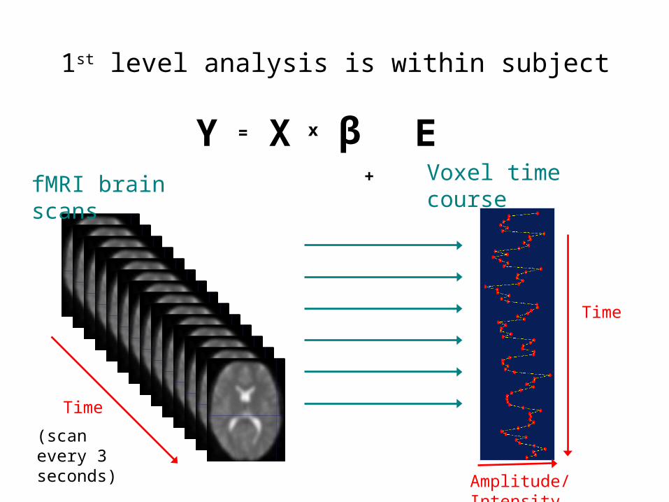
1st level analysis is within subject
Time
(scan every 3 seconds)
fMRI brain scans Voxel time course
Amplitude/Intensity
Time
Y = X x β + E
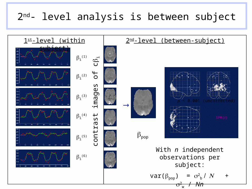
2nd- level analysis is between subject
p < 0.001 (uncorrected)
SPM{t}
1st-level (within subject) 2nd-level (between-subject)
cont
rast
imag
es o
f cb i
bi(1)
bi(2)
bi(3)
bi(4)
bi(5)
bi(6)
bpop
With n independent observations per subject:
var(bpop) = 2b / N + 2
w / Nn
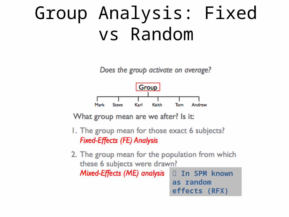
Group Analysis: Fixed vs Random
In SPM known as random effects (RFX)

Consider a single voxel for 12 subjects
Effect Sizes = [4, 3, 2, 1, 1, 2, ....]sw = [0.9, 1.2, 1.5, 0.5, 0.4, 0.7, ....]
• Group mean, m=2.67• Mean within subject variance sw =1.04• Between subject (std dev), sb =1.07

Group Analysis: Fixed-effects
Compare group effect with within-subject variance
NO inferences about the population
Because between subject variance not considered, you may get larger effects

FFX calculation
• Calculate a within subject variance over time
sw = [0.9, 1.2, 1.5, 0.5, 0.4, 0.7, 0.8, 2.1, 1.8, 0.8, 0.7, 1.1]
• Mean effect, m=2.67• Mean sw =1.04
Standard Error Mean (SEMW) = sw /sqrt(N)=0.04
• t=m/SEMW=62.7
• p=10-51

Fixed-effects Analysis in SPM
Fixed-effects• multi-subject 1st level design • each subjects entered as
separate sessions• create contrast across all
subjectsc = [ 1 -1 1 -1 1 -1 1 -1 1 -1 ]
• perform one sample t-test
Multisubject 1st level : 5 subjects x 1 run each
Subject 1
Subject 2
Subject 3
Subject 4
Subject 5

Group analysis: Random-effects
Takes into account between-subject variance
CAN make inferences about the population
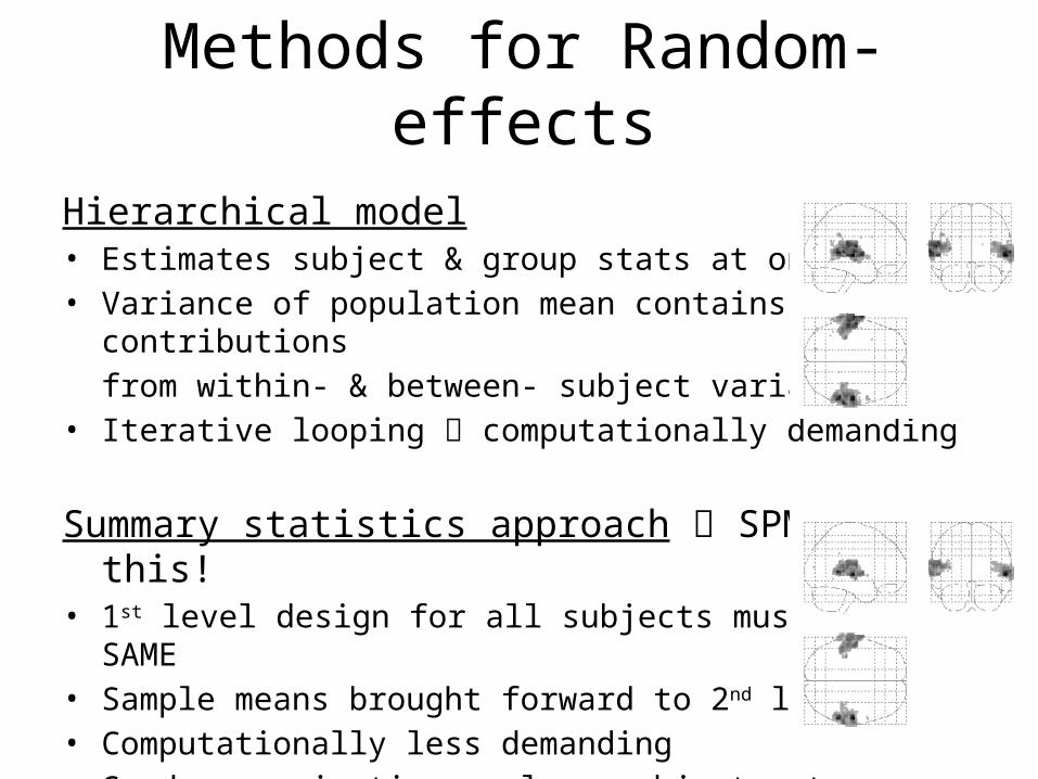
Methods for Random-effects
Hierarchical model• Estimates subject & group stats at once• Variance of population mean contains contributions
from within- & between- subject variance• Iterative looping computationally demanding
Summary statistics approach SPM uses this!• 1st level design for all subjects must be the SAME• Sample means brought forward to 2nd level• Computationally less demanding• Good approximation, unless subject extreme outlier

Random Effects Analysis- Summary Statistic Approach
• For group of N=12 subjects effect sizes are
c= [3, 4, 2, 1, 1, 2, 3, 3, 3, 2, 4, 4]
Group effect (mean), m=2.67Between subject variability (stand dev), sb =1.07
• This is called a Random Effects Analysis (RFX) because we are comparing the group effect to the between-subject variability.
• This is also known as a summary statistic approach because we are summarising the response of each subject by a single summary statistic – their effect size.
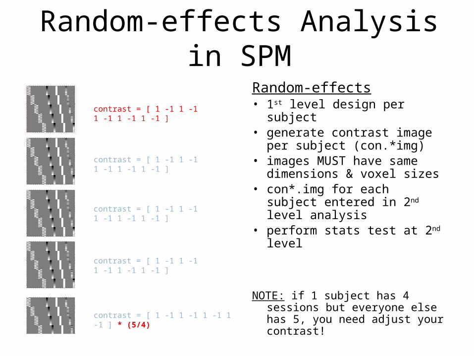
Random-effects Analysis in SPM
Random-effects• 1st level design per subject • generate contrast image per
subject (con.*img)• images MUST have same
dimensions & voxel sizes• con*.img for each subject
entered in 2nd level analysis• perform stats test at 2nd level
NOTE: if 1 subject has 4 sessions but everyone else has 5, you need adjust your contrast!
Subject #2 x 5 runs (1st level)
Subject #3 x 5 runs (1st level)
Subject #4 x 5 runs (1st level)
Subject #5 x 4 runs (1st level)
contrast = [ 1 -1 1 -1 1 -1 1 -1 1 -1 ]
contrast = [ 1 -1 1 -1 1 -1 1 -1 1 -1 ]
contrast = [ 1 -1 1 -1 1 -1 1 -1 1 -1 ]
contrast = [ 1 -1 1 -1 1 -1 1 -1 1 -1 ]
contrast = [ 1 -1 1 -1 1 -1 1 -1 ] * (5/4)
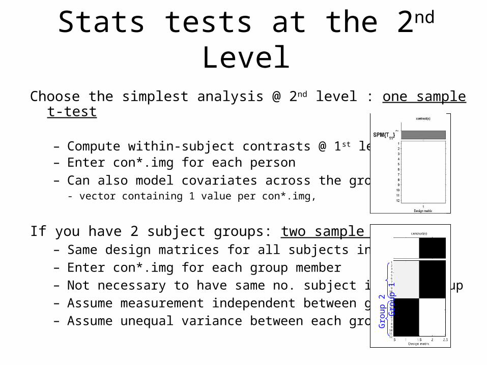
Choose the simplest analysis @ 2nd level : one sample t-test
– Compute within-subject contrasts @ 1st level– Enter con*.img for each person– Can also model covariates across the group
- vector containing 1 value per con*.img,
If you have 2 subject groups: two sample t-test– Same design matrices for all subjects in a group– Enter con*.img for each group member– Not necessary to have same no. subject in each group– Assume measurement independent between groups– Assume unequal variance between each group
Stats tests at the 2nd Level
123456789
101112
123456789
101112
Grou
p 2
G
roup
1

Stats tests at the 2nd Level
If you have no other choice: ANOVA
• Designs are much more complexe.g. within-subject ANOVA need covariate per subject
• BEWARE sphericity assumptions may be violated, need to account for
• Better approach:– generate main effects & interaction
contrasts at 1st levelc = [ 1 1 -1 -1] ; c = [ 1 -1 1 -1 ] ; c = [ 1 -1 -1 1]
– use separate t-tests at the 2nd level
Subj
ect 1
Subj
ect 2
Subj
ect 3
Subj
ect 4
Subj
ect 5
Subj
ect 6
Subj
ect 7
Subj
ect 8
Subj
ect 9
Subj
ect 1
0Su
bjec
t 11
Subj
ect 1
2
2x2 designAx Ao Bx Bo
One sample t-test equivalents:
A>B x>o A(x>o)>B(x>o)con.*imgs con.*imgs con.*imgs c = [ 1 1 -1 -1] c= [ 1 -1 1 -1] c = [ 1 -1 -1 1]
Setting up models for group analysis
• Overview – One sample T test– Two sample T test– Paired T test– One way ANOVA– One way ANOVA-repeated measure– Two way ANOVA– Difference between SPM and other software
packages
Setting up second level models
DATA VECTOR = DESIGN MATRIX * PARAMETERS + ERROR VECTOR
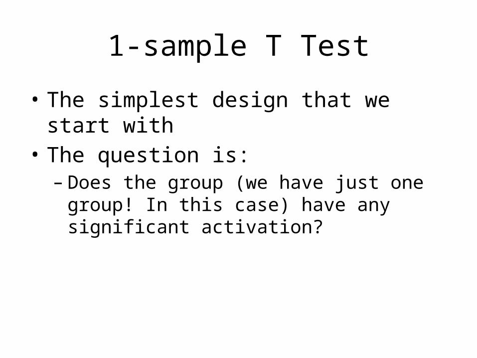
1-sample T Test
• The simplest design that we start with• The question is:
– Does the group (we have just one group! In this case) have any significant activation?

1-sample T Test
Xβ=
Design matrix for 10 subjects
β C=[1]

Two sample T-test in SPM
• There are different ways of constructing design matrix for a two sample T-test
• Example:– 5 subjects in group 1 – 5 subjects in group 2– Question: are these two groups have significant
difference in brain activation?
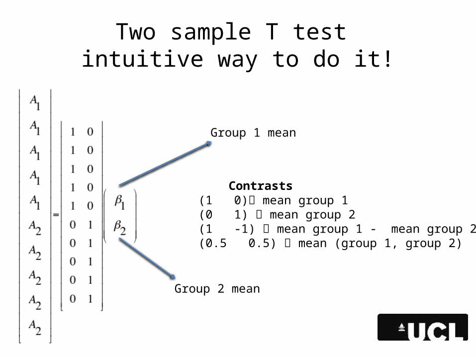
Two sample T test intuitive way to do it!
Group 1 mean
Group 2 mean
(1 0) mean group 1(0 1) mean group 2(1 -1) mean group 1 - mean group 2(0.5 0.5) mean (group 1, group 2)
Contrasts

2 sample T testsecond way to do it
β1
β2
Group 1 mean
Group 2 mean
β2+

What’s the contrast for mean of group 1 being significantly different from zero

Group 2 mean different from zero
Mean G1 – Mean G2
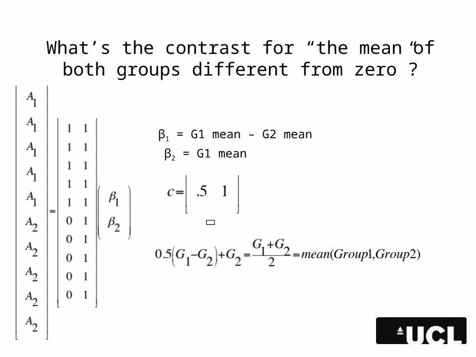
What’s the contrast for “the mean of both groups different from zero”?
β2 = G1 mean
β1 = G1 mean – G2 mean
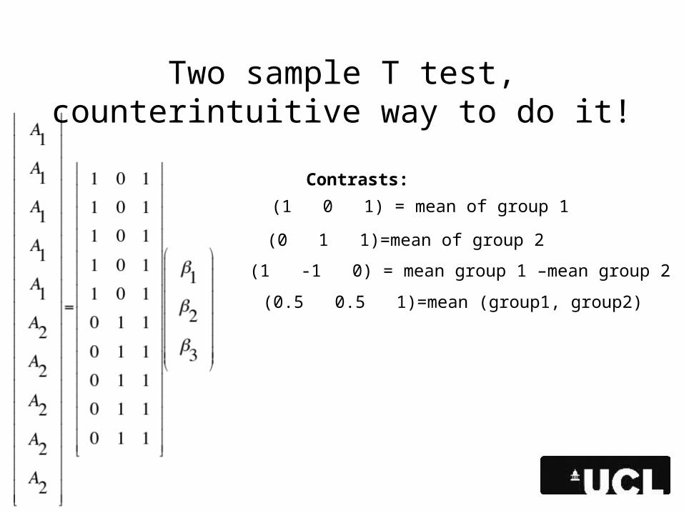
Two sample T test, counterintuitive way to do it!
Contrasts:(1 0 1) = mean of group 1
(0 1 1)=mean of group 2
(1 -1 0) = mean group 1 –mean group 2
(0.5 0.5 1)=mean (group1, group2)

Non estimable contrast (SPM)Rank deficient (FSL)
Suppose we do this contrast:C=[1 1 -1]

Paired T test
• The model underlying the paired T test model is just an extension of two sample T test
• It assumes that scans come in pairs• One scan in each pair• Each pair is a group• The mean of each pair is modeled separately
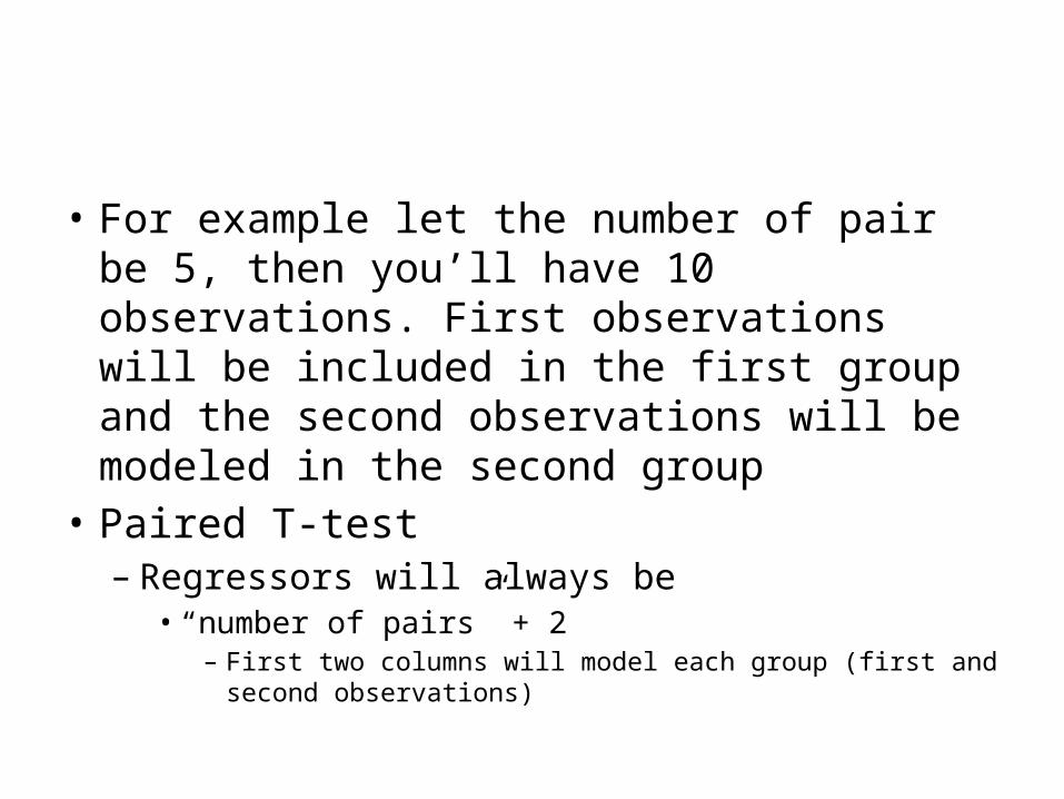
• For example let the number of pair be 5, then you’ll have 10 observations. First observations will be included in the first group and the second observations will be modeled in the second group
• Paired T-test – Regressors will always be
• “number of pairs” + 2– First two columns will model each group (first and second
observations)

Paired T test- SPM way to do it
Ho=β1<β2
C=[-1 1 0 0 0 0 0]

Paire
d T
Test
-FSL
-Fre
esur
fer w
ay to
do
itH0: Paired difference = 0
C=[1 0 0 0 0 ]

There is another way to do paired T test and that’s
when you model pairs at the first level and do a one
sample t test at the second level
ANOVA
• Factorial designs are mainstay of scientific experiments
• Data are collected for each level/factor • They should be analyzed using analysis of
variance• They are being used for the analysis in PET, EEG,
MEG, and fMRI– For PET analysis ANOVA is usually being done at first
level
fMRI and factorial design
• Factorial designs are cost efficient• ANOVA is used in second level• ANOVA uses F-tests to assess main effects and
also interaction effects based on the experimental design
• The level of a factor is also sometimes referred to as a ‘treatment’ or a ‘group’ and each factor/level combination is referred to as a ‘cell’ or ‘condition’. (SPM book)

One way between subject ANOVA
• Consider a one-way ANOVA with 4 groups and each group having 3 subjects, 12 observations in total
• SPM rule– Number of regressors = number of groups

One way between subject ANOVA-SPM
G1
G2
G3
G4
Mean of all
H0: G1=G2=G3=G4
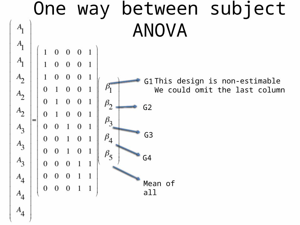
One way between subject ANOVA
G1
G2
G3
G4
Mean of all
This design is non-estimableWe could omit the last column
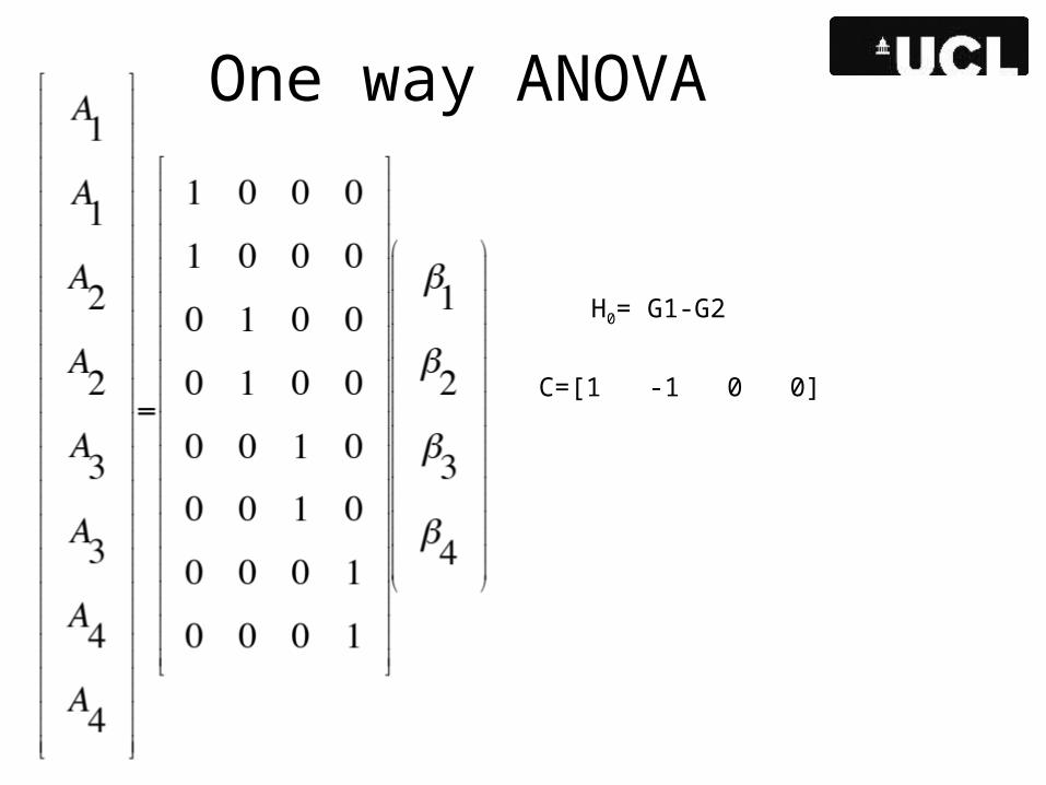
One way ANOVA
H0= G1-G2
C=[1 -1 0 0]

One way ANOVA
H0= G1=G2=G3=G4=0
c=
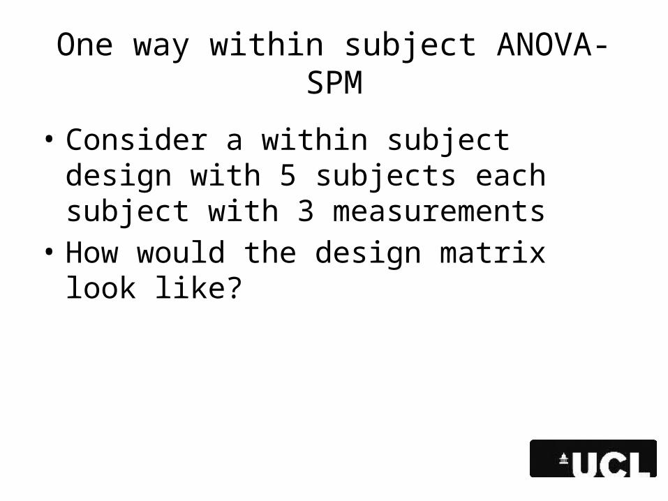
One way within subject ANOVA-SPM
• Consider a within subject design with 5 subjects each subject with 3 measurements
• How would the design matrix look like?

5 subjects each subject with 3 measurements
The first 3 columns are treatment effects andOther columns are subject effects
Contrast for group 1 different than 0C=[1 0 0 0 0 0 0 0]
Contrast for group 3 > group 1C=[-1 0 1 0 0 0 0 0]

Non-sphericity
• Due to the nature of the levels in an experiment, it may be the case that if a subject responds strongly to level i, he may respond strongly to level j. In other words, there may be a correlation between responses.
• The presence of non-spherecity makes us less assured of the significance of the data, so we use Greenhouse-Geisser correction.
• Mauchly’s sphericity test

Two Way within subject ANOVA
• It consist of main effects and interactions. Each factor has an associated main effect, which is the difference between the levels of that factor, averaging over the levels of all other factors. Each pair of factors has an associated interaction. Interactions represent the degree to which the effect of one factor depends on the levels of the other factor(s). A two-way ANOVA thus has two main effects and one interaction.
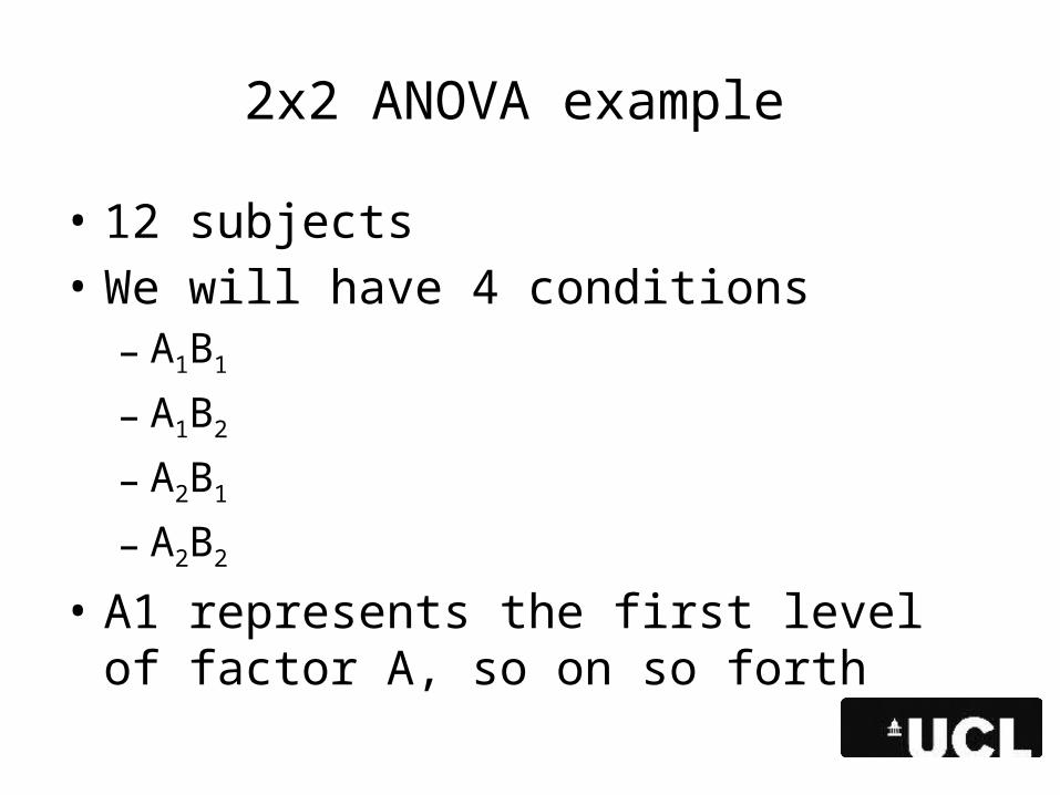
2x2 ANOVA example
• 12 subjects• We will have 4 conditions
– A1B1
– A1B2
– A2B1
– A2B2
• A1 represents the first level of factor A, so on so forth

2x2 ANOVA
The rows are ordered all subjects for cell A1B1, all for A1B2 etc
Difference of different levels of A, averagedOver B main effect of A

Design matrix for 2x2 ANOVA, rotated
White 1Gray 0Black -1
Main effect A Main effect BInteraction effect Subject effects

2x2 ANOVA model
• Main effect of A– [1 0 0 0]
• Main effect of B– [0 1 0 0]
• Interaction, AXB– [0 0 1 0]

Mumford rules for One way ANOVA-FSL
• Number of regressors for a factor = Number of levels – 1
• Factor with 4 levels– Xi=
• 1 if subject is from level i• -1 if case from level 4• 0 otherwise
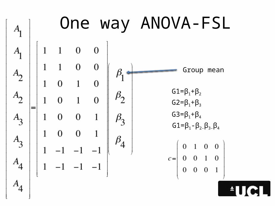
One way ANOVA-FSL
Group mean
G1=β1+β2
G3=β1+β4
G1=β1-β2-β3-β4
G2=β1+β3
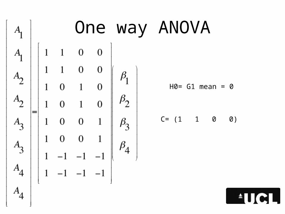
One way ANOVA
H0= G1 mean = 0
C= (1 1 0 0)

Is group 1 different from 4?
Contrast for group 1 is:(1 1 0 0)
Contrast for group 4 is(1 -1 -1 -1)
Contrast for G1-G4 will be(0 2 1 1)

2 Way ANOVA-FSL
• Mumford rules:– Setting up design matrix – Xi =
• 1 if case from level I• -1 if case from level n• 0 otherwise
• A has 3 levels, so 2 regressors• B has 2 levels, so 1 regressors

Two Way ANOVA-FSL
A B AB
Main factor A effect
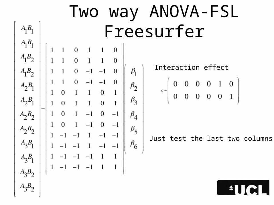
Two way ANOVA-FSL Freesurfer
Interaction effect
Just test the last two columns!

Two Way ANOVA
A1B1? Cell mean

The End