“2cee”A 21st Century

Effort Estimation MethodologyTim MenziesDan Baker

tim@menzies.usdbaker6@mix.wvu.edu

Jairus HihnKaren Lum

jhihn@jpl.nasa.govktlum@jpl.nasa.gov

22nd International Forum on COCOMO and Systems/Software Cost Modeling (2007)

2cee 2

Our Journey

• It became quickly apparent in the early stages of our research task that there was a major disconnect between the techniques used by estimation practitioners and the numerous ideas being addressed in the research community

• It also became clear that many fundamental estimation questions were not being addressed– What is a models real estimation uncertainty?– How many records required to calibrate?

• Answers have varied from 10-20 just for intercept and slope• If we do not have enough data what is the impact on model uncertainty

– Data is expensive to collect and maintain so want to keep cost drivers and effort multipliers as few as possible

• But what are the right ones?• When should we build domain specific models?

– What are the best functional forms?– What are the best ways to tune/calibrate a model?

2cee 3

Our Journey Continued• Data mining techniques provided us with the

rigorous tool set we needed to explore the many dimension of the problem we were addressing in a repeatable manner – Different Calibration and Validation Datasets– Analyze standard and non-standard models– Perform exhaustive searches over all parameters

and records in order to guide data pruning • Rows (Stratification)• Columns (variable reduction)

– Measure model performance by multiple measures– We have even been able to determine what

performance measures are best

2cee 4

Some Things We Learned Along the Way

2cee 5

Local Calibration Does Not Always Improve Performance

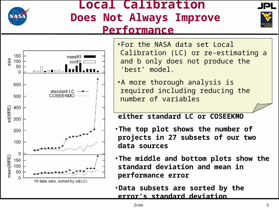
• Effort models were learned via either standard LC or COSEEKMO

• The top plot shows the number of projects in 27 subsets of our two data sources

• The middle and bottom plots show the standard deviation and mean in performance error

• Data subsets are sorted by the error’s standard deviation

• For the NASA data set Local Calibration (LC) or re-estimating a and b only does not produce the ‘best’ model.

• A more thorough analysis is required including reducing the number of variables

2cee 6

Stratification Does Not Always Improve Performance

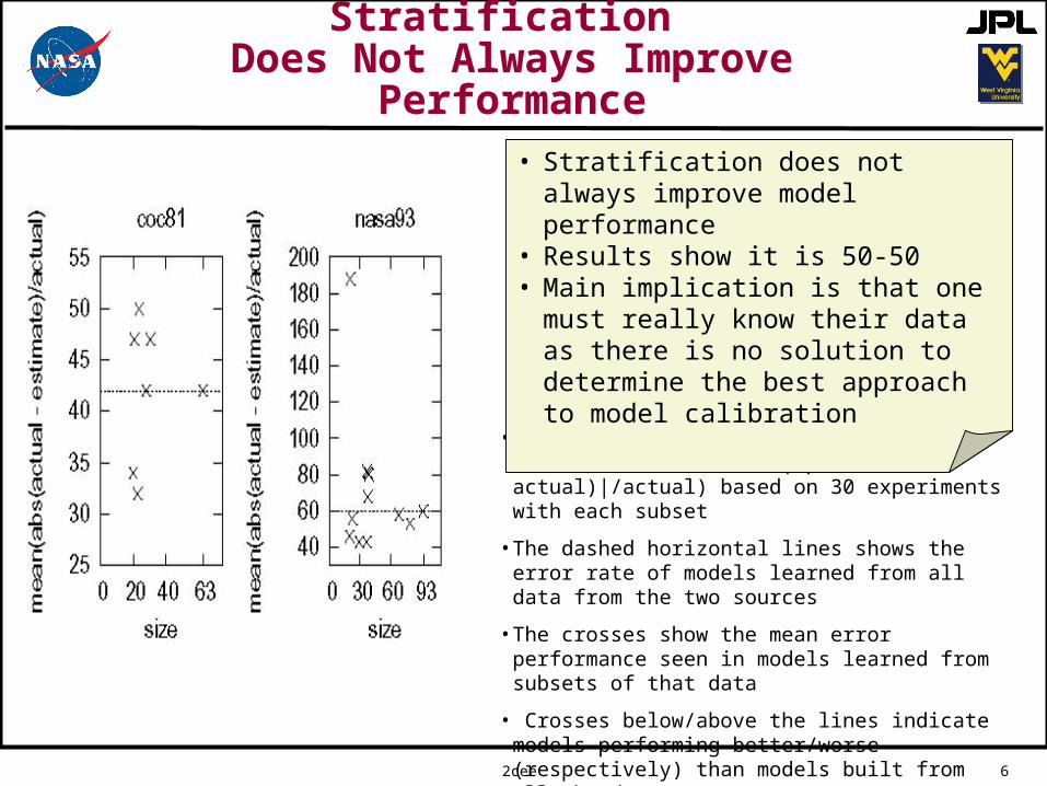
• The plots show mean performance error (i.e. |(predicted − actual)|/actual) based on 30 experiments with each subset

• The dashed horizontal lines shows the error rate of models learned from all data from the two sources

• The crosses show the mean error performance seen in models learned from subsets of that data

• Crosses below/above the lines indicate models performing better/worse (respectively) than models built from all the data

• Stratification does not always improve model performance

• Results show it is 50-50• Main implication is that one must really

know their data as there is no solution to determine the best approach to model calibration

2cee 7

Cost Driver Instability

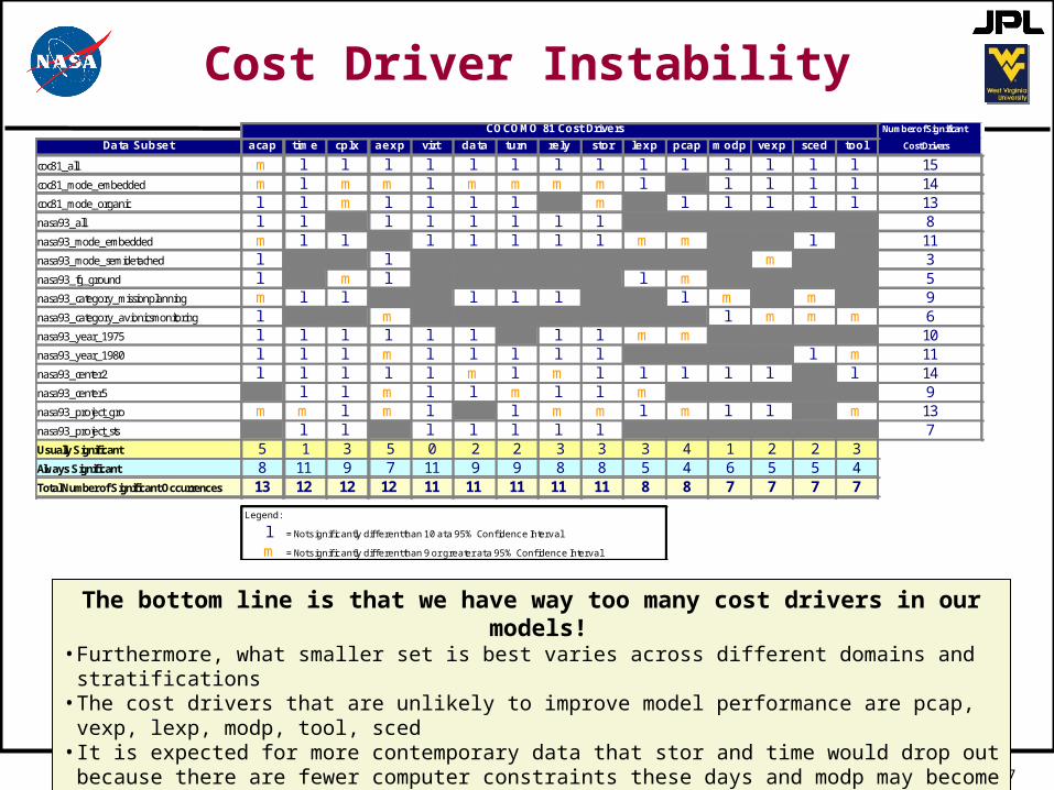
Data Subset acap time cplx aexp virt data turn rely stor lexp pcap modp vexp sced tool

coc81_all m l l l l l l l l l l l l l l 15coc81_mode_embedded m l m m l m m m m l l l l l 14coc81_mode_organic l l m l l l l m l l l l l 13nasa93_all l l l l l l l l 8nasa93_mode_embedded m l l l l l l l m m l 11nasa93_mode_semidetached l l m 3nasa93_fg_ground l m l l m 5nasa93_category_missionplanning m l l l l l l m m 9nasa93_category_avionicsmonitoring l m l m m m 6nasa93_year_1975 l l l l l l l l m m 10nasa93_year_1980 l l l m l l l l l l m 11nasa93_center2 l l l l l m l m l l l l l l 14nasa93_center5 l l m l l m l l m 9nasa93_project_gro m m l m l l m m l m l l m 13nasa93_project_sts l l l l l l l 7Usually Significant 5 1 3 5 0 2 2 3 3 3 4 1 2 2 3Always Significant 8 11 9 7 11 9 9 8 8 5 4 6 5 5 4Total Number of Significant Occurrences 13 12 12 12 11 11 11 11 11 8 8 7 7 7 7

Legend:

l = Not significantly different than 10 at a 95% Confidence Interval

m = Not significantly different than 9 or greater at a 95% Confidence Interval

COCOMO 81 Cost Drivers Number of Significant

Cost Drivers

The bottom line is that we have way too many cost drivers in our models!• Furthermore, what smaller set is best varies across different domains and stratifications• The cost drivers that are unlikely to improve model performance are pcap, vexp, lexp, modp, tool,

sced• It is expected for more contemporary data that stor and time would drop out because there are fewer

computer constraints these days and modp may become more significant

2cee 8

Some Good News

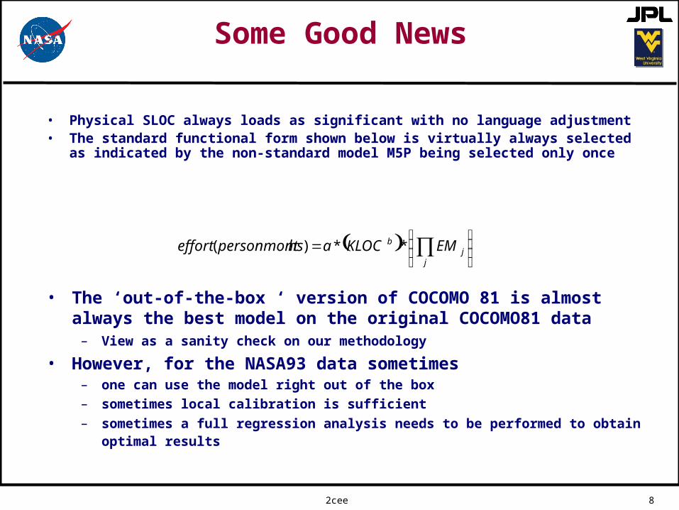
• Physical SLOC always loads as significant with no language adjustment• The standard functional form shown below is virtually always selected

as indicated by the non-standard model M5P being selected only once

( ) ⎟⎟⎠

⎞⎜⎜⎝

⎛= ∏

jj

b EMKLOCahspersonmonteffort **)(

• The ‘out-of-the-box ‘ version of COCOMO 81 is almost always the best model on the original COCOMO81 data

– View as a sanity check on our methodology

• However, for the NASA93 data sometimes – one can use the model right out of the box – sometimes local calibration is sufficient– sometimes a full regression analysis needs to be performed to obtain

optimal results

2cee 9

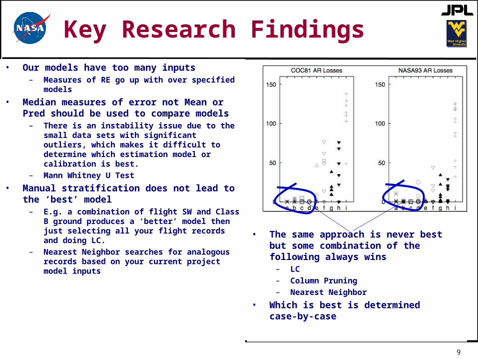
• The same approach is never best but some combination of the following always wins

– LC – Column Pruning– Nearest Neighbor

• Which is best is determined case-by-case

Key Research Findings• Our models have too many inputs

– Measures of RE go up with over specified models

• Median measures of error not Mean or Pred should be used to compare models

– There is an instability issue due to the small data sets with significant outliers, which makes it difficult to determine which estimation model or calibration is best.

– Mann Whitney U Test

• Manual stratification does not lead to the ‘best’ model

– E.g. a combination of flight SW and Class B ground produces a ‘better’ model then just selecting all your flight records and doing LC.

– Nearest Neighbor searches for analogous records based on your current project model inputs

2cee 10

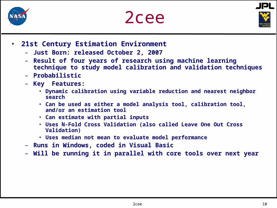
2cee• 21st Century Estimation Environment

– Just Born: released October 2, 2007– Result of four years of research using machine learning technique

to study model calibration and validation techniques – Probabilistic – Key Features:

• Dynamic calibration using variable reduction and nearest neighbor search

• Can be used as either a model analysis tool, calibration tool, and/or an estimation tool

• Can estimate with partial inputs • Uses N-Fold Cross Validation (also called Leave One Out Cross

Validation)• Uses median not mean to evaluate model performance

– Runs in Windows, coded in Visual Basic– Will be running it in parallel with core tools over next year

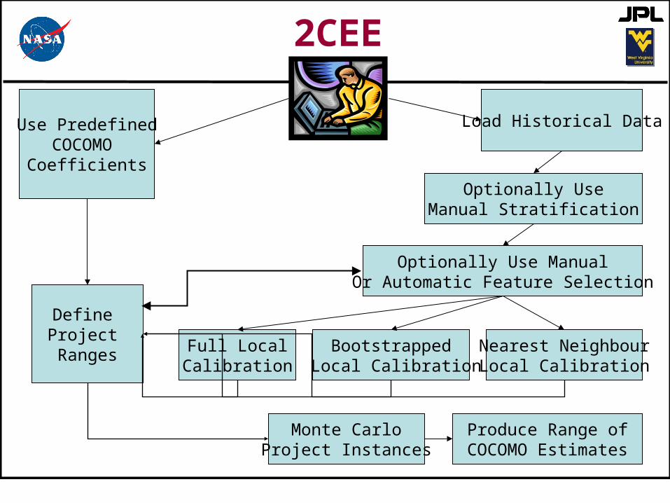
Load Historical DataUse PredefinedCOCOMO Coefficients

Bootstrapped Local Calibration

Full LocalCalibration

Nearest NeighbourLocal Calibration

Optionally Use ManualOr Automatic Feature Selection

Optionally UseManual Stratification

2CEE

Define Project Ranges

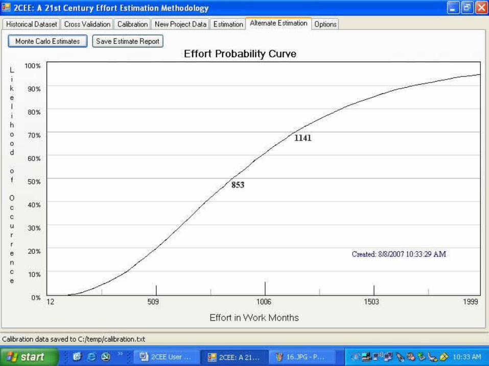
Monte CarloProject Instances

Produce Range ofCOCOMO Estimates

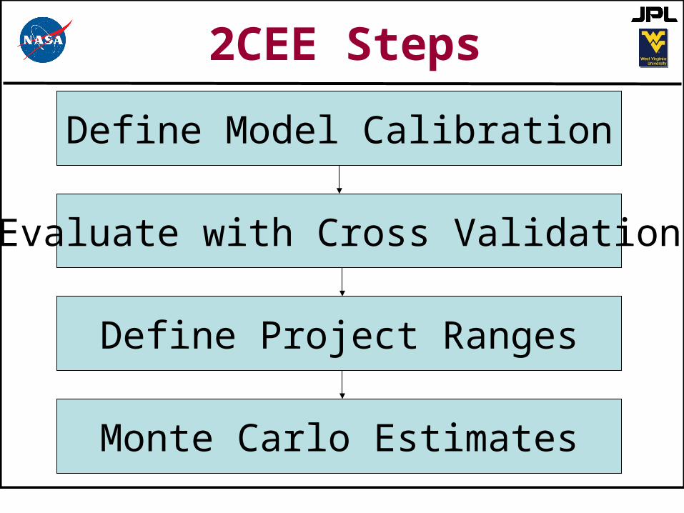
2CEE Steps

Define Model Calibration

Evaluate with Cross Validation

Define Project Ranges

Monte Carlo Estimates

2cee 14

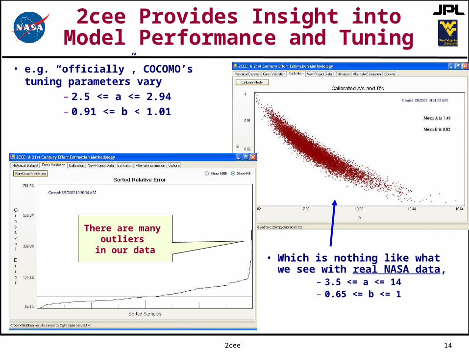
2cee Provides Insight into Model Performance and Tuning

• e.g. “officially”, COCOMO’s tuning parameters vary

– 2.5 <= a <= 2.94– 0.91 <= b < 1.01

• Which is nothing like whatwe see with real NASA data,

– 3.5 <= a <= 14– 0.65 <= b <= 1

There are many outliers

in our data

2cee 16

Karen will be available at the tool fair

Stop in and take a lookunder the hood

2cee 17

Bibliography

Current Research Publications

Selecting Best Practices for Effort Estimation, IEEE Transactions On Software Engineering, Nov 2006. (Menzies, Chen, Hihn, Lum)

Evidence-Based Cost Estimation for Better-Quality Software, IEEE Software, July/August 2006. (Menzies and Hihn )

Studies in Software Cost Model Behavior:Do We Really Understand Cost Model Performance?, Proceedings of the ISPA International Conference 2006, Seattle, WA. (Lum, Hihn, Menzies) (Best Paper Award)

Simple Software Cost Analysis: Safe or Unsafe?, Proceedings of the International Workshop on Predictor Models in Software Engineering (PROMISE 2005), St Louis, MS, 14 June 2005. (Menzies, Port, Hihn , Chen)

Feature Subset Selection Improves Software Cost Estimation. (PROMISE 2005), St Louis, MS, 14 June 2005. (Chen, Menzies, Port, Boehm)

Validation methods for calibrating software effort models, ICSE 2005 Proceedings, May 2005, St Louis, MS. May 2005. (Menzies, Port, Hihn, Chen)

Specialization and Extrapolation of Software Cost Models, Proceeding in Automation in Software Engineering Conference, Nov 2005. (Menzies, Chen, Port, Hihn)

Finding the Right Data for Software Cost Modeling, IEEE Software, Nov/Dec 2005. (Chen, Menzies, Port, Boehm)

2cee 18

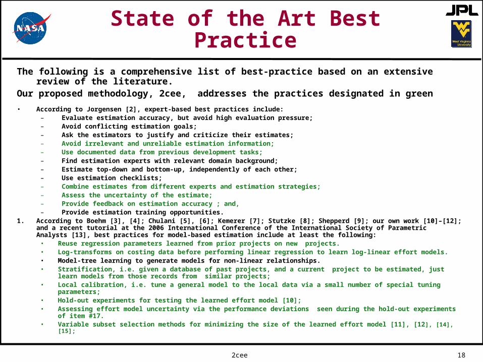
State of the Art Best Practice

The following is a comprehensive list of best-practice based on an extensive review of the literature.

Our proposed methodology, 2cee, addresses the practices designated in green

• According to Jorgensen [2], expert-based best practices include: – Evaluate estimation accuracy, but avoid high evaluation pressure; – Avoid conflicting estimation goals; – Ask the estimators to justify and criticize their estimates; – Avoid irrelevant and unreliable estimation information; – Use documented data from previous development tasks; – Find estimation experts with relevant domain background; – Estimate top-down and bottom-up, independently of each other; – Use estimation checklists; – Combine estimates from different experts and estimation strategies; – Assess the uncertainty of the estimate; – Provide feedback on estimation accuracy ; and, – Provide estimation training opportunities.

1. According to Boehm [3], [4]; Chulani [5], [6]; Kemerer [7]; Stutzke [8]; Shepperd [9]; our own work [10]–[12]; and a recent tutorial at the 2006 International Conference of the International Society of Parametric Analysts [13], best practices for model-based estimation include at least the following:

• Reuse regression parameters learned from prior projects on new projects. • Log-transforms on costing data before performing linear regression to learn log-linear effort models. • Model-tree learning to generate models for non-linear relationships. • Stratification, i.e. given a database of past projects, and a current project to be estimated, just learn

models from those records from similar projects; • Local calibration, i.e. tune a general model to the local data via a small number of special tuning

parameters; • Hold-out experiments for testing the learned effort model [10]; • Assessing effort model uncertainty via the performance deviations seen during the hold-out experiments

of item #17. • Variable subset selection methods for minimizing the size of the learned effort model [11], [12], [14], [15];