2.1 Merton’s firm value model

• Built upon a stochastic process of the firm’s value. [This is notthe book value of the assets, but more like the value that thefirm can be sold – including good view.]

• Aim to provide a link between the prices of equity and all debtinstruments issued by one particular firm

• Default occurs when the firm value falls to a low level such thatthe issuer cannot meet the par payment at maturity or couponpayments.

Potential applications

1. Relative value trading between shares and debt of one particularissuer.

2. Default risk assessment of a firm based upon its share price andfundamental (balance sheet) data.

Credit valuation model

1. Credit risk should be measured in terms of probabilities andmathematical expectations, rather than assessed by qualitativeratings.

2. Credit risk model should be based on current, rather than histor-ical measurements. The relevant variables are the actual marketvalues rather than accounting values. It should reflect the de-velopment in the borrower’s credit standing through time.

3. An assessment of the future earning power of the firm, com-pany’s operations, projection of cash flows, etc., has alreadybeen made by the aggregate of the market participants in thestock market. The stock price will be the first to reflect thechanging prospects. The challenge is how to interpret thechanging share prices properly.

4. The various liabilities of a firm are claims on the firm’s value,which often take the form of options, so the credit model shouldbe consistent with the theory of option pricing.

Firm value

• The value of a firm is the value of its business as a going con-cern. The firm’s business constitutes its assets, and the presentassessment of the future returns from the firm’s business con-stitutes the current value of the firm’s assets.

• The value of the firm’s assets is different from the bottom lineon the firm’s balance sheet. When the firm is bought or sold, thevalue traded is the ongoing business. The difference betweenthe amount paid for that value and the amount of book assetsis usually accounted for as the “good will”.

• The value of the firm’s assets can be measured by the price atwhich the total of the firm’s liabilities can be bought or sold.The various liabilities of the firm are claims on its assets. Theclaimants may include the debt holders, equity holder, etc.

• market value of firm asset

= market value of equity + market value of bonds

= share price times no. of shares + sum of market bond prices

Assumptions in the Merton model

1. The firm asset value Vt evolves according to

dV

V= µ dt + σ dZ

µ = instantaneous expected rate of return.

2. The liabilities of the firm consist only of a single debt with facevalue F . The debt is assumed not to have coupon nor embeddedoption feature.

3. The debt is viewed as a contingent claim on the firm’s asset.Default can be triggered only at maturity and this occurs whenVT < F .

4. Upon default, the firm is liquidated at zero cost and all theproceeds from liquidation are transferred to the debt holder.

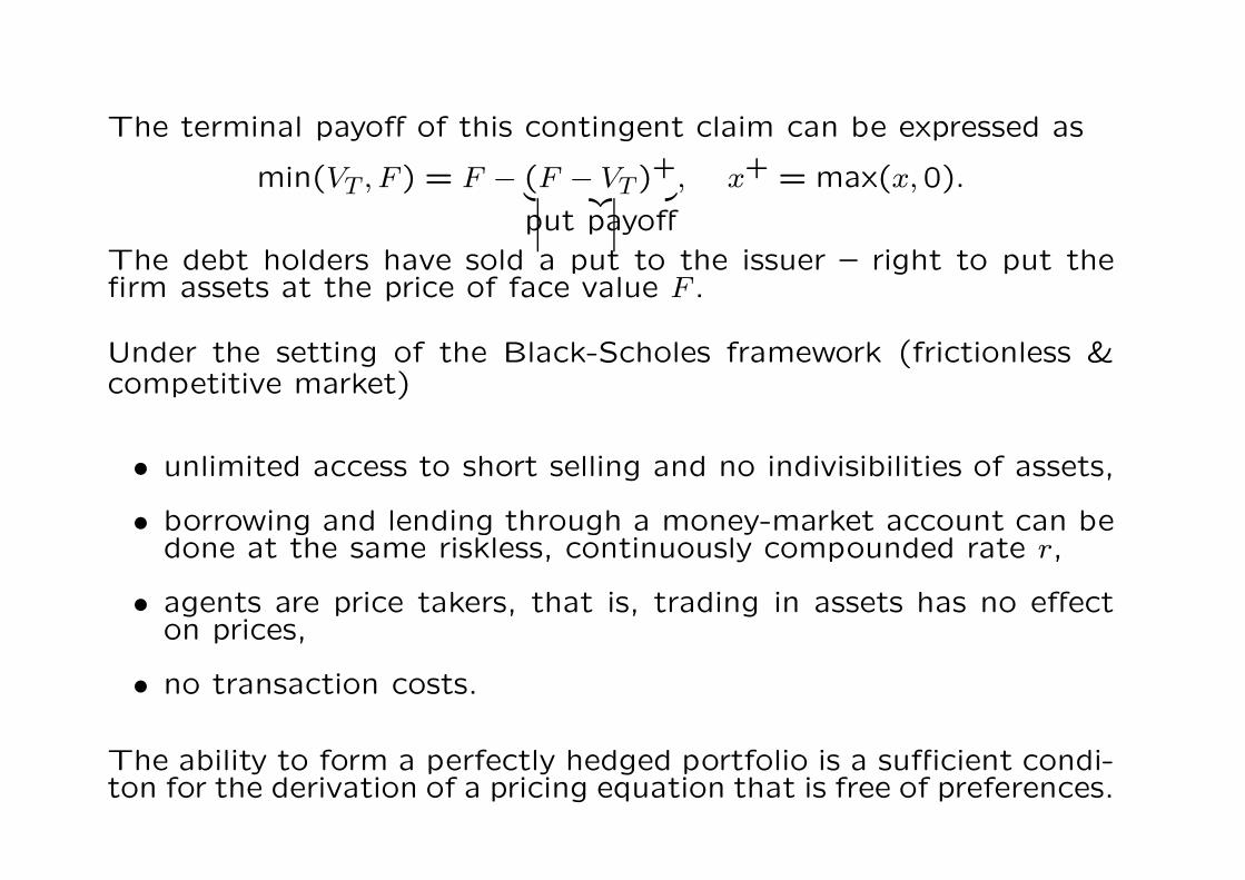
The terminal payoff of this contingent claim can be expressed as

min(VT , F) = F − (F − VT )+︸ ︷︷ ︸put payoff

, x+ = max(x,0).

The debt holders have sold a put to the issuer – right to put thefirm assets at the price of face value F .

Under the setting of the Black-Scholes framework (frictionless &competitive market)

• unlimited access to short selling and no indivisibilities of assets,

• borrowing and lending through a money-market account can bedone at the same riskless, continuously compounded rate r,

• agents are price takers, that is, trading in assets has no effecton prices,

• no transaction costs.

The ability to form a perfectly hedged portfolio is a sufficient condi-ton for the derivation of a pricing equation that is free of preferences.

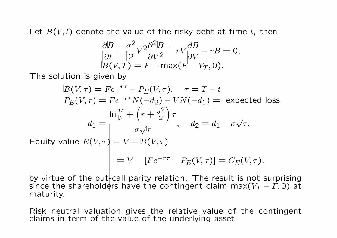
Let B(V, t) denote the value of the risky debt at time t, then

∂B

∂t+

σ2

2V 2∂2B

∂V 2+ rV

∂B

∂V− rB = 0,

B(V, T ) = F − max(F − VT ,0).

The solution is given by

B(V, τ) = Fe−rτ − PE(V, τ), τ = T − t

PE(V, τ) = Fe−rτN(−d2) − V N(−d1) = expected loss

d1 =ln V

F +(r + σ2

2

)τ

σ√

τ, d2 = d1 − σ

√τ .

Equity value E(V, τ) = V − B(V, τ)

= V − [Fe−rτ − PE(V, τ)] = CE(V, τ),

by virtue of the put-call parity relation. The result is not surprisingsince the shareholders have the contingent claim max(VT − F,0) atmaturity.

Risk neutral valuation gives the relative value of the contingentclaims in term of the value of the underlying asset.

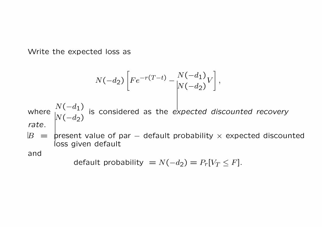
Write the expected loss as

N(−d2)

[Fe−r(T−t) −

N(−d1)

N(−d2)V

],

whereN(−d1)

N(−d2)is considered as the expected discounted recovery

rate.

B = present value of par − default probability × expected discountedloss given default

anddefault probability = N(−d2) = Pr[VT ≤ F ].

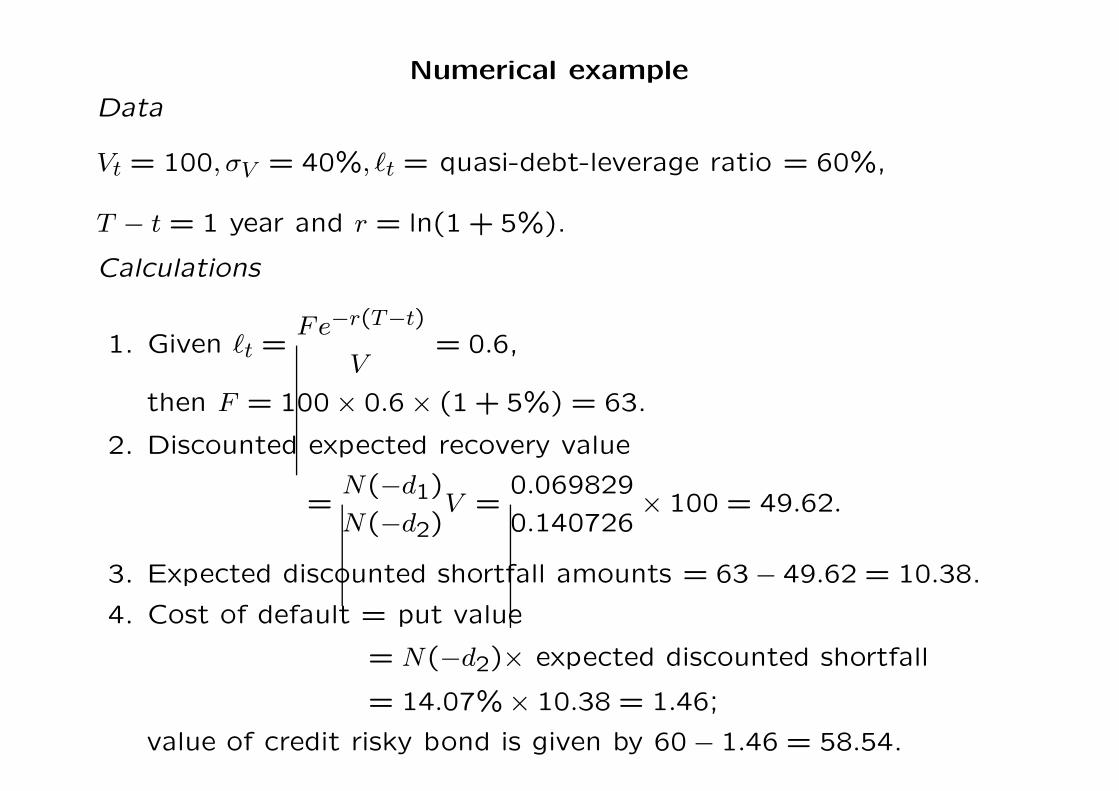
Numerical example

Data

Vt = 100, σV = 40%, `t = quasi-debt-leverage ratio = 60%,

T − t = 1 year and r = ln(1 + 5%).

Calculations

1. Given `t =Fe−r(T−t)

V= 0.6,

then F = 100 × 0.6 × (1 + 5%) = 63.

2. Discounted expected recovery value

=N(−d1)

N(−d2)V =

0.069829

0.140726× 100 = 49.62.

3. Expected discounted shortfall amounts = 63 − 49.62 = 10.38.

4. Cost of default = put value

= N(−d2)× expected discounted shortfall

= 14.07%× 10.38 = 1.46;

value of credit risky bond is given by 60 − 1.46 = 58.54.

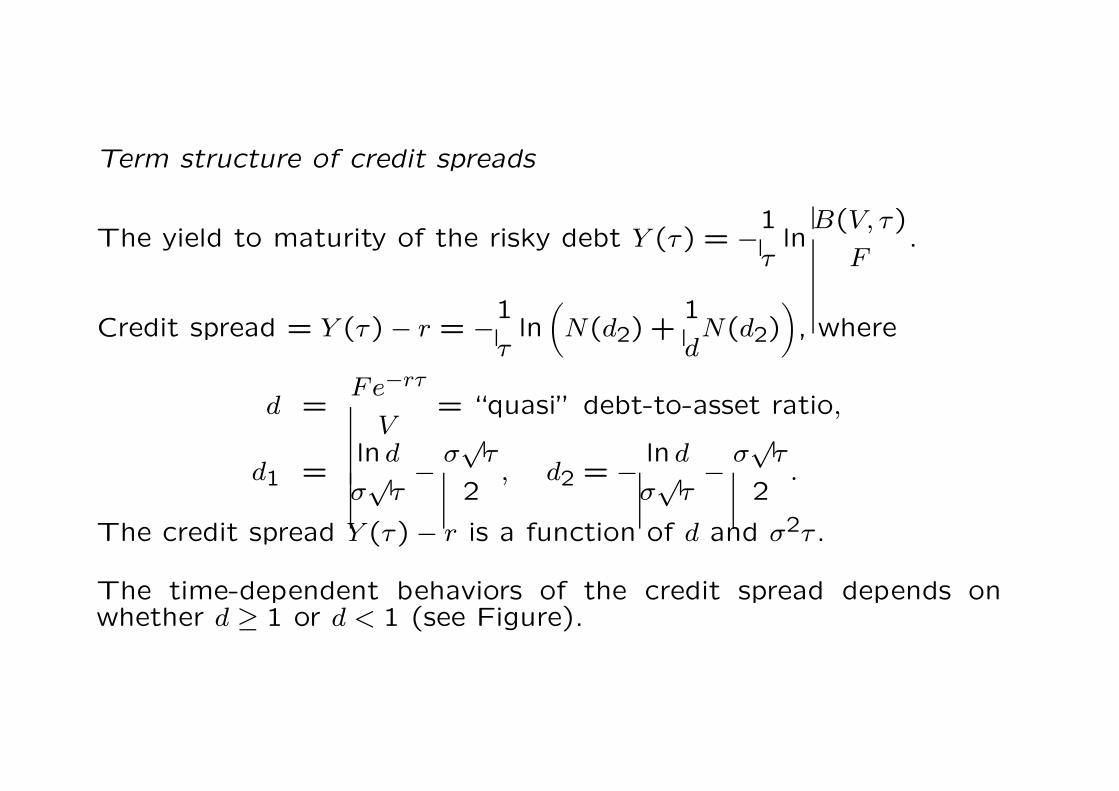
Term structure of credit spreads

The yield to maturity of the risky debt Y (τ) = −1

τln

B(V, τ)

F.

Credit spread = Y (τ) − r = −1

τln(N(d2) +

1

dN(d2)

), where

d =Fe−rτ

V= “quasi” debt-to-asset ratio,

d1 =ln d

σ√

τ−

σ√

τ

2, d2 = −

ln d

σ√

τ−

σ√

τ

2.

The credit spread Y (τ) − r is a function of d and σ2τ .

The time-dependent behaviors of the credit spread depends onwhether d ≥ 1 or d < 1 (see Figure).

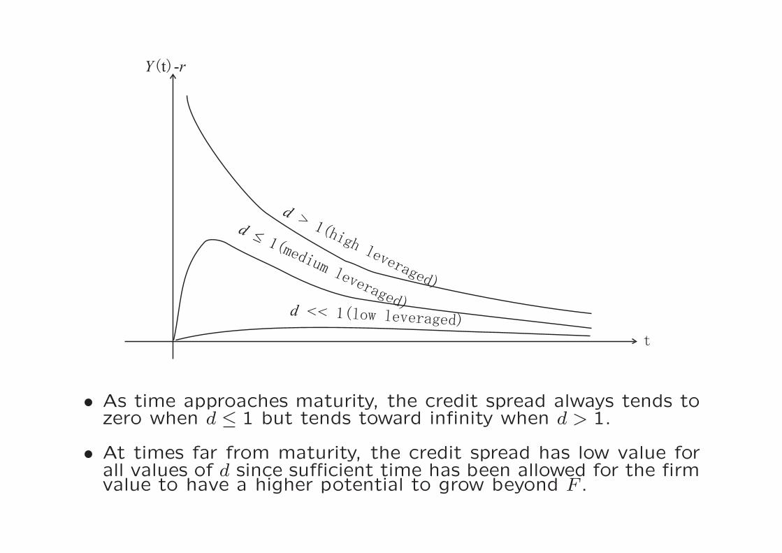
• As time approaches maturity, the credit spread always tends tozero when d ≤ 1 but tends toward infinity when d > 1.

• At times far from maturity, the credit spread has low value forall values of d since sufficient time has been allowed for the firmvalue to have a higher potential to grow beyond F .

Time dependent behaviors of credit spreads

• Downward-sloping for highly leveraged firms.

• Humped shape for medium leveraged firms.

• Upward-sloping for low leveraged firms.

Possible explanation

• For high-quality bonds, credit spreads widen as maturity in-creases since the upside potential is limited and the downsiderisk is substantial.

Remark

Most banking regulations do not recognize the term structure ofcredit spreads. When allocating capital to cover potential defaultsand credit downgrades, a one-year risky bond is treated the sameas a ten-year counterpart.

Shortcomings

1. Default can never occur by surprise since the firm value is as-sumed to follow a diffusion process – may be partially remediedby introducing jump effect into the firm value process.

2. Actual spreads are larger than those predicted by Merton’s model.

3. Default premiums are shown to be inversely related to firm sizeas revealed from empirical studies. In Merton’s model, Y (τ)− ris a function of d and σ2τ only.

Reference

H.Y. Wong and Y.K. Kwok, “Jump diffusion model for risky debts:quanlity spread differentials,” International Journal of Theoreticaland Applied Finance, vol. 6(6) (2003) p.655-662.

Example – Risky commodity-linked bond

• A silver mining company offered bond issues backed by silver.Each $1,000 bond is linked to 50 ounces of silver, pays a couponrate of 8.5% and has a maturity of 15 years.

• At maturity, the company guarantees to pay the holders either$1,000 or the market value of 50 ounces of silver.

Rationale The issuer is willing to share the potential price appre-ciation in exchange for a lower coupon rate or otherfavorable bond indentures.

Terminal payoff of bond value

B(V, S, T ) = min(V, F + max(S − F,0)),where V is the firm value, r is the interest rate, S is the value of 50ounces of silver, F is the face value.

2.2 Extensions of structural approach of pricing risking debts

1. Interest rate uncertainty

Debts are relatively long-term interest rate sensitive instruments.The assumption of constant rates is embarrassing.

• Jump-diffusion process of the firm value.• Allows for a jump process to shock the firm value process.• Remedy the realistic small short-maturity spreads in pure dif-

fusion model. Default may occur by surprise.

2. Bankruptcy– triggering mechanism

Black-Cox (1976) assume a cut-off level whereby intertemporaldefault can occur. The cut-off may be considered as a safetycovenant which protects bondholder or liability level for the firmbelow which the firm bankrupts.

3. Deviation from the strict priority rule

Empirical studies show that the absolute priority rule is enforcedin only 25% of corporate bankruptcy cases. The write-downof creditor claims is usually the outcome of a bargaining pro-cess which results in shifts of gains and losses among corporateclaimants relative to their contractual rights.

Quality spread differentials between fixed rate debtand floating rate debt

• In fixed rate debts, the par paid at maturity is fixed.

• A floating rate debt is similar to a money market account, wherethe par at maturity is the sum of principal and accured interests.The amount of accrued interests depends on the realization ofthe stochastic interest rate over the life of bond.

What is the appropriate proportion of debts into either fixed rateor flating rate debts?

1. Balance sheet duration2. Current interest rate environment3. Peer group practices.

Whether the default premiums demanded by investors are equal forboth types of debts?

Related question: Deos the swap rate in an interest rate swapdepend on which party is serving as the fixedrate payer?

Empirical studies reveal that the yeeld premiums for fixed rate debtsare in general higher than those for floating rate debts. Why? Onthe other hand, when the yield curve is upward sloping, floating ratedebt holders should demand a higher floating spread.

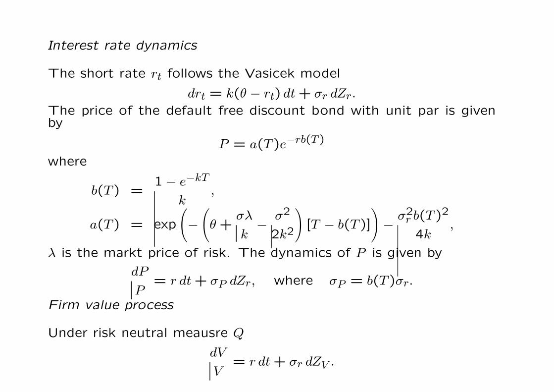
Interest rate dynamics

The short rate rt follows the Vasicek model

drt = k(θ − rt) dt + σr dZr.

The price of the default free discount bond with unit par is givenby

P = a(T )e−rb(T )

where

b(T ) =1 − e−kT

k,

a(T ) = exp

(−(

θ +σλ

k−

σ2

2k2

)[T − b(T )]

)−

σ2r b(T )2

4k,

λ is the markt price of risk. The dynamics of P is given by

dP

P= r dt + σP dZr, where σP = b(T )σr.

Firm value process

Under risk neutral meausre Q

dV

V= r dt + σr dZV .

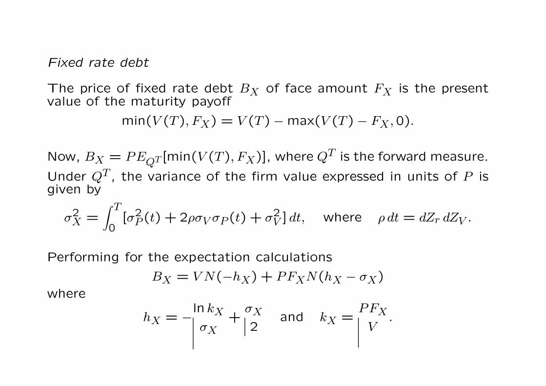
Fixed rate debt

The price of fixed rate debt BX of face amount FX is the presentvalue of the maturity payoff

min(V (T ), FX) = V (T ) − max(V (T ) − FX,0).

Now, BX = PEQT [min(V (T ), FX)], where QT is the forward measure.

Under QT , the variance of the firm value expressed in units of P isgiven by

σ2X =

∫ T

0[σ2

P (t) + 2ρσV σP (t) + σ2V ] dt, where ρ dt = dZr dZV .

Performing for the expectation calculations

BX = V N(−hX) + PFXN(hX − σX)

where

hX = −ln kX

σX+

σX

2and kX =

PFX

V.

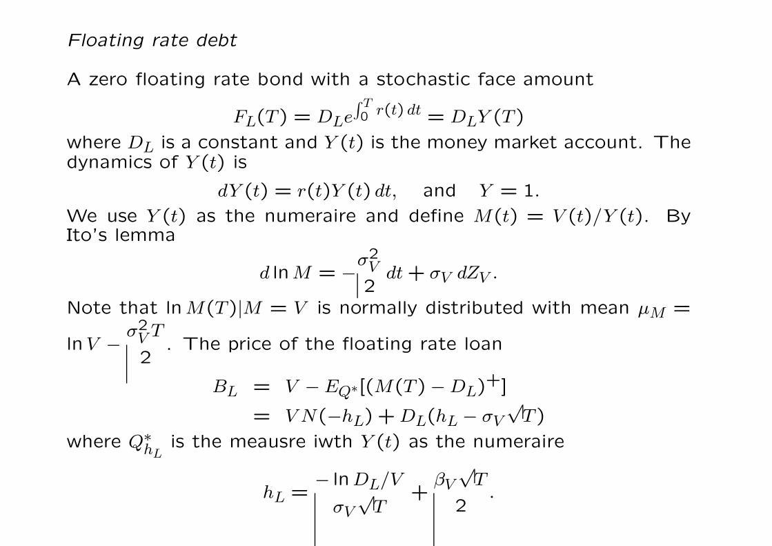
Floating rate debt

A zero floating rate bond with a stochastic face amount

FL(T ) = DLe∫ T0 r(t) dt = DLY (T )

where DL is a constant and Y (t) is the money market account. Thedynamics of Y (t) is

dY (t) = r(t)Y (t) dt, and Y = 1.

We use Y (t) as the numeraire and define M(t) = V (t)/Y (t). ByIto’s lemma

d lnM = −σ2

V

2dt + σV dZV .

Note that lnM(T )|M = V is normally distributed with mean µM =

lnV −σ2

V T

2. The price of the floating rate loan

BL = V − EQ∗[(M(T ) − DL)+]

= V N(−hL) + DL(hL − σV

√T )

where Q∗hL

is the meausre iwth Y (t) as the numeraire

hL =− lnDL/V

σV

√T

+βV

√T

2.

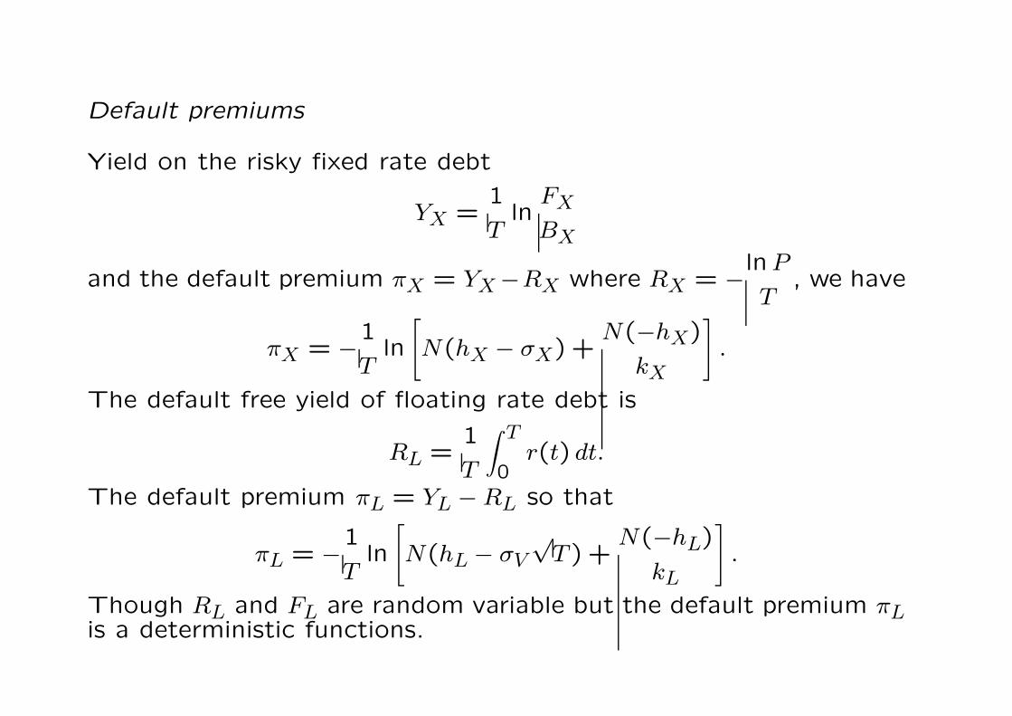
Default premiums

Yield on the risky fixed rate debt

YX =1

Tln

FX

BX

and the default premium πX = YX −RX where RX = −lnP

T, we have

πX = −1

Tln

[N(hX − σX) +

N(−hX)

kX

].

The default free yield of floating rate debt is

RL =1

T

∫ T

0r(t) dt.

The default premium πL = YL − RL so that

πL = −1

Tln

[N(hL − σV

√T ) +

N(−hL)

kL

].

Though RL and FL are random variable but the default premium πLis a deterministic functions.

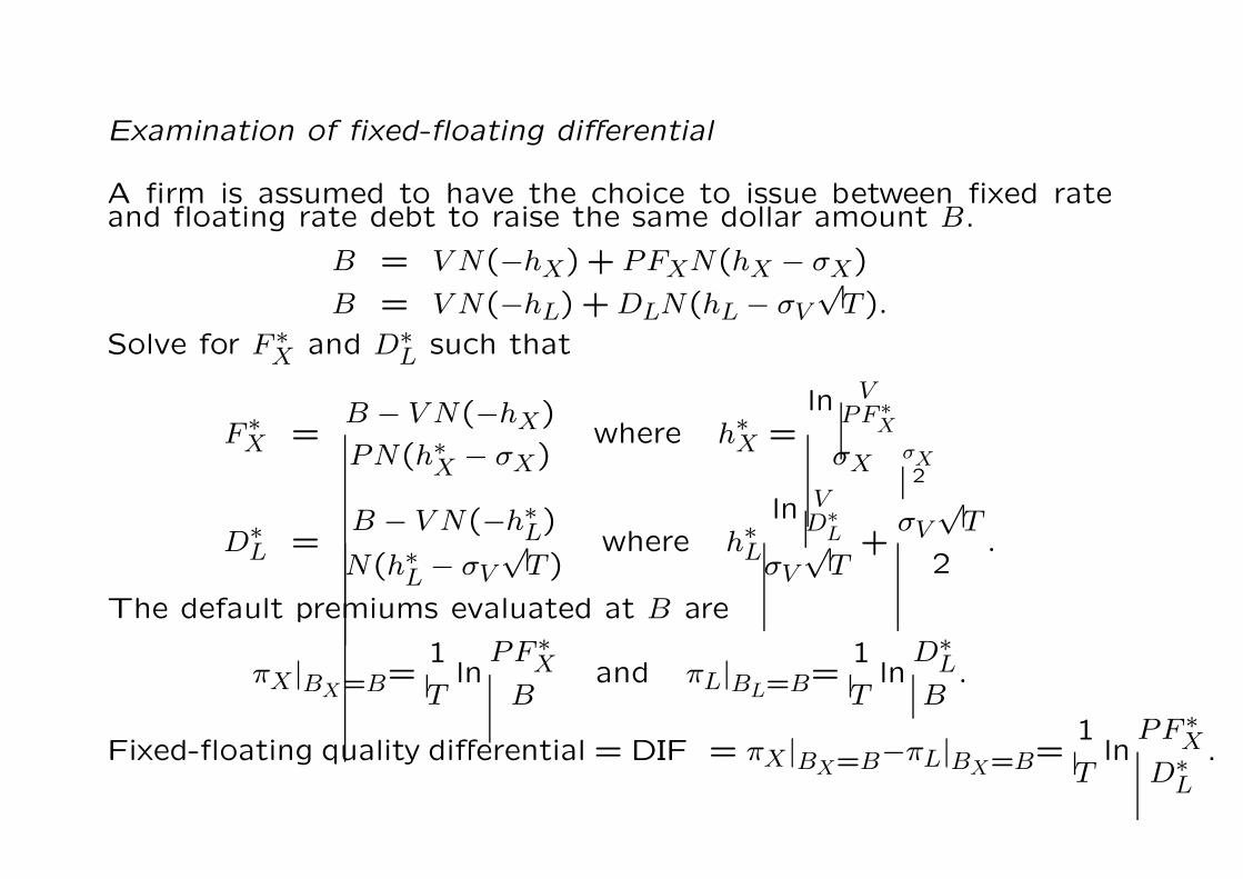
Examination of fixed-floating differential

A firm is assumed to have the choice to issue between fixed rateand floating rate debt to raise the same dollar amount B.

B = V N(−hX) + PFXN(hX − σX)

B = V N(−hL) + DLN(hL − σV

√T ).

Solve for F ∗X and D∗

L such that

F ∗X =

B − V N(−hX)

PN(h∗X − σX)

where h∗X =

ln VPF ∗

X

σXσX2

D∗L =

B − V N(−h∗L)

N(h∗L − σV

√T )

where h∗L

ln VD∗

L

σV

√T

+σV

√T

2.

The default premiums evaluated at B are

πX |BX=B=1

Tln

PF ∗X

Band πL|BL=B=

1

Tln

D∗L

B.

Fixed-floating quality differential = DIF = πX |BX=B−πL|BX=B=1

Tln

PF ∗X

D∗L

.

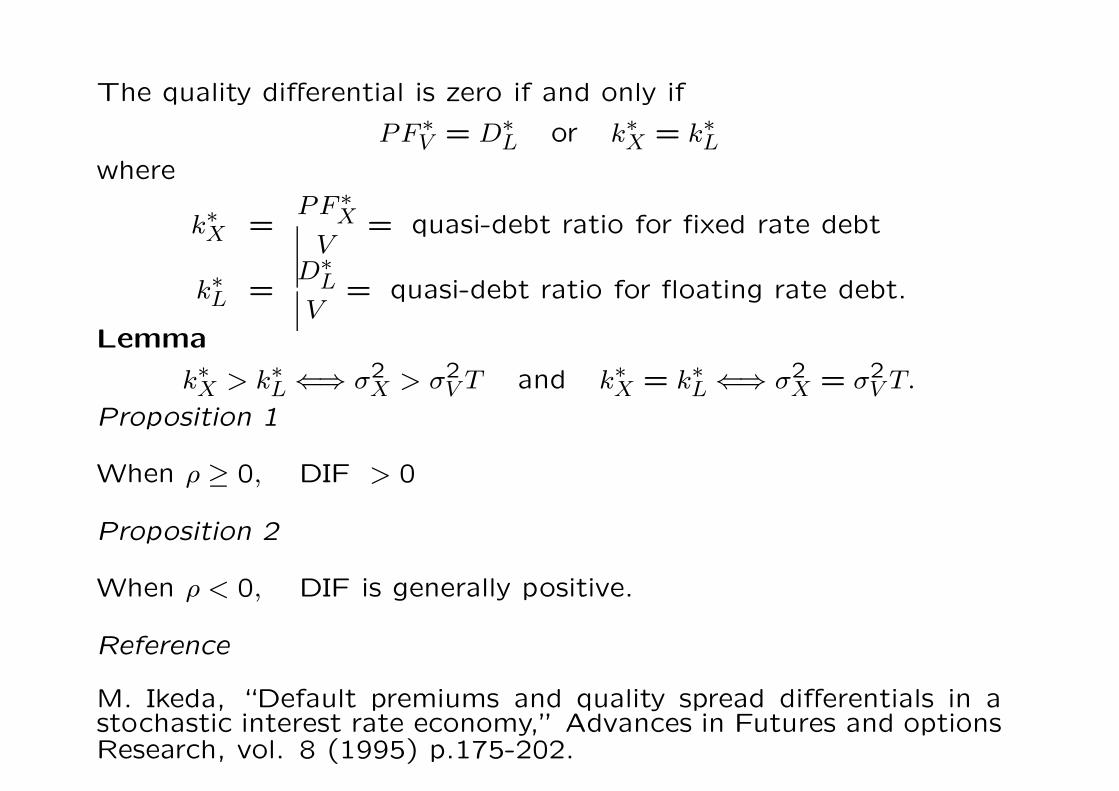
The quality differential is zero if and only if

PF ∗V = D∗

L or k∗X = k∗Lwhere

k∗X =PF ∗

X

V= quasi-debt ratio for fixed rate debt

k∗L =D∗

L

V= quasi-debt ratio for floating rate debt.

Lemma

k∗X > k∗L ⇐⇒ σ2X > σ2

V T and k∗X = k∗L ⇐⇒ σ2X = σ2

V T.

Proposition 1

When ρ ≥ 0, DIF > 0

Proposition 2

When ρ < 0, DIF is generally positive.

Reference

M. Ikeda, “Default premiums and quality spread differentials in astochastic interest rate economy,” Advances in Futures and optionsResearch, vol. 8 (1995) p.175-202.

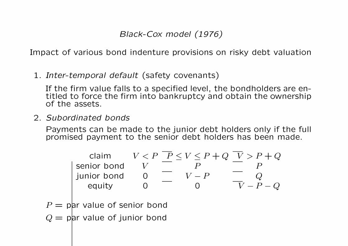
Black-Cox model (1976)

Impact of various bond indenture provisions on risky debt valuation

1. Inter-temporal default (safety covenants)

If the firm value falls to a specified level, the bondholders are en-titled to force the firm into bankruptcy and obtain the ownershipof the assets.

2. Subordinated bonds

Payments can be made to the junior debt holders only if the fullpromised payment to the senior debt holders has been made.

claim V < P P ≤ V ≤ P + Q V > P + Qsenior bond V P Pjunior bond 0 V − P Q

equity 0 0 V − P − Q

P = par value of senior bond

Q = par value of junior bond

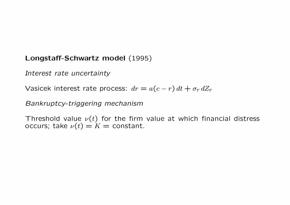
Longstaff-Schwartz model (1995)

Interest rate uncertainty

Vasicek interest rate process: dr = a(c − r) dt + σr dZr

Bankruptcy-triggering mechanism

Threshold value ν(t) for the firm value at which financial distressoccurs; take ν(t) = K = constant.

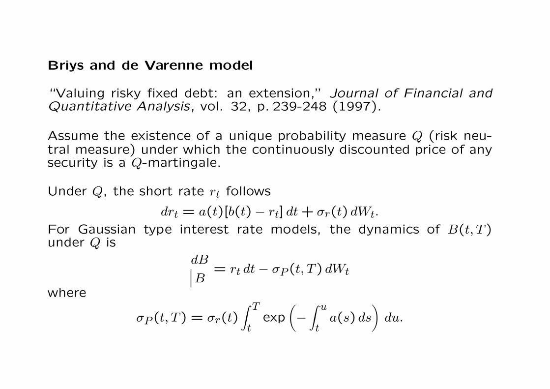
Briys and de Varenne model

“Valuing risky fixed debt: an extension,” Journal of Financial andQuantitative Analysis, vol. 32, p. 239-248 (1997).

Assume the existence of a unique probability measure Q (risk neu-tral measure) under which the continuously discounted price of anysecurity is a Q-martingale.

Under Q, the short rate rt follows

drt = a(t)[b(t)− rt] dt + σr(t) dWt.

For Gaussian type interest rate models, the dynamics of B(t, T )under Q is

dB

B= rt dt − σP (t, T ) dWt

where

σP (t, T ) = σr(t)∫ T

texp

(−∫ u

ta(s) ds

)du.

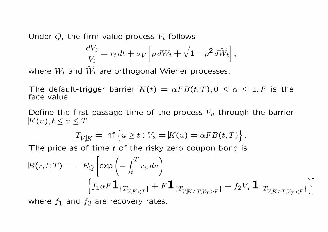
Under Q, the firm value process Vt follows

dVt

Vt= rt dt + σV

[ρ dWt +

√1 − ρ2 dWt

],

where Wt and Wt are orthogonal Wiener processes.

The default-trigger barrier K(t) = αFB(t, T ), 0 ≤ α ≤ 1, F is theface value.

Define the first passage time of the process Vu through the barrierK(u), t ≤ u ≤ T .

TV,K = inf{u ≥ t : Vu = K(u) = αFB(t, T )

}.

The price as of time t of the risky zero coupon bond is

B(r, t;T ) = EQ

[exp

(−∫ T

tru du

)

{f1αF1{T

V,K<T} + F1{T

V,K≥T,VT ≥F} + f2VT1{T

V,K≥T,VT <F}

}]

where f1 and f2 are recovery rates.

Advantages

The term structure of corporate spreads is affected by the presenceof safety covenant and the violations of the absolute priority rule.

• Larger corporate spreads than those derived by Merton’s model.

• Corporate spreads will exhibit more amplex structures since thereare more parameters in the model.

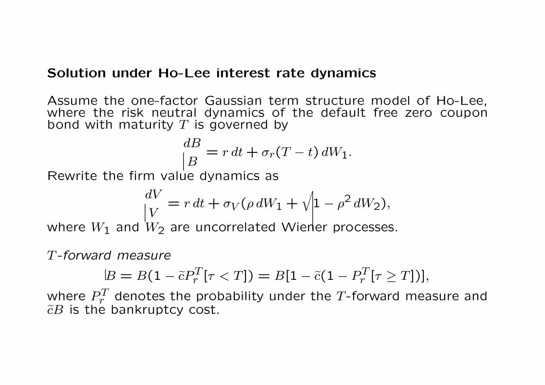
Solution under Ho-Lee interest rate dynamics

Assume the one-factor Gaussian term structure model of Ho-Lee,where the risk neutral dynamics of the default free zero couponbond with maturity T is governed by

dB

B= r dt + σr(T − t) dW1.

Rewrite the firm value dynamics as

dV

V= r dt + σV (ρ dW1 +

√1 − ρ2 dW2),

where W1 and W2 are uncorrelated Wiener processes.

T -forward measure

B = B(1 − cPTr [τ < T ]) = B[1 − c(1 − PT

r [τ ≥ T ])],

where PTr denotes the probability under the T -forward measure and

cB is the bankruptcy cost.

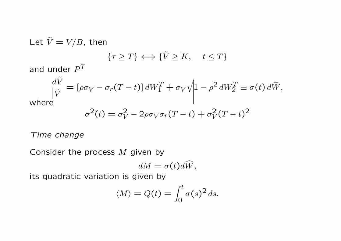
Let V = V/B, then

{τ ≥ T} ⇐⇒ {V ≥ K, t ≤ T}and under PT

dV

V= [ρσV − σr(T − t)] dWT

1 + σV

√1 − ρ2 dWT

2 ≡ σ(t) dW ,

where

σ2(t) = σ2V − 2ρσV σr(T − t) + σ2

V (T − t)2

Time change

Consider the process M given by

dM = σ(t)dW ,

its quadratic variation is given by

〈M〉 = Q(t) =∫ t

0σ(s)2 ds.

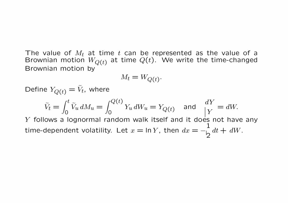
The value of Mt at time t can be represented as the value of aBrownian motion WQ(t) at time Q(t). We write the time-changedBrownian motion by

Mt = WQ(t).

Define YQ(t) = Vt, where

Vt =∫ t

0Vu dMu =

∫ Q(t)

0Yu dWu = YQ(t) and

dY

Y= dW.

Y follows a lognormal random walk itself and it does not have any

time-dependent volatility. Let x = lnY , then dx = −1

2dt + dW .

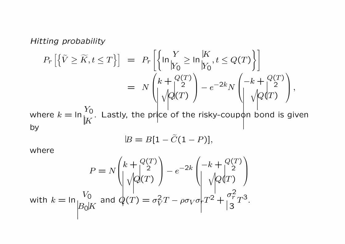
Hitting probability

Pr

[{V ≥ K, t ≤ T

}]= Pr

[{ln

Y

Y0≥ ln

K

Y0, t ≤ Q(T )

}]

= N

k + Q(T )2√

Q(T )

− e−2kN

−k + Q(T )

2√Q(T )

,

where k = lnY0

K. Lastly, the price of the risky-coupon bond is given

by

B = B[1 − C(1 − P)],where

P = N

k + Q(T )2√

Q(T )

− e−2k

−k + Q(T )

2√Q(T )

with k = lnV0

B0Kand Q(T ) = σ2

V T − ρσV σrT2 +σ2

r

3T3.

Towards dynamic capital structure: Stationary leverage ratios

“Do credit spreads reflect stationary leverage ratio?” P. Collin-Dufresne and R.S. Goldstein, Journal of Finance, vol. 56 (5),p.1929-1957 (2001).

Background

• Firms adjust outstanding debt levels in response to changes infirm value, thus generating mean-reverting leverage ratios.

• Develop a structural model of default with stochastic interestrates that generates stationary leverage ratios (exogenous as-sumption on future leverage).

• Empirical studies show the support for the existence of targetleverage ratios within an industry. Theoretical dynamic modelsof optimal capital structure find that firm value is maximizedwhen a firm acts to keep its leverage ratio within a certainband.

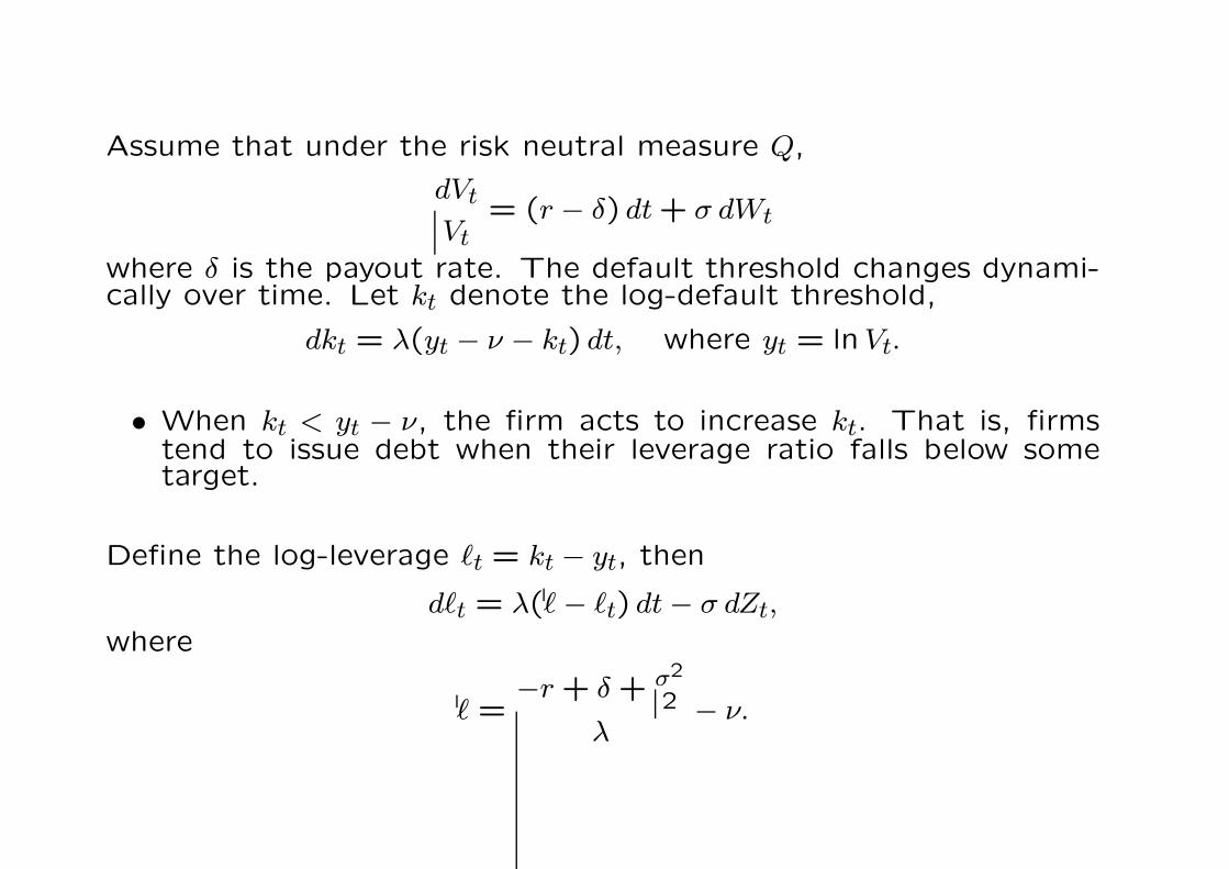
Assume that under the risk neutral measure Q,

dVt

Vt= (r − δ) dt + σ dWt

where δ is the payout rate. The default threshold changes dynami-cally over time. Let kt denote the log-default threshold,

dkt = λ(yt − ν − kt) dt, where yt = lnVt.

• When kt < yt − ν, the firm acts to increase kt. That is, firmstend to issue debt when their leverage ratio falls below sometarget.

Define the log-leverage `t = kt − yt, then

d`t = λ(` − `t) dt − σ dZt,

where

` =−r + δ + σ2

2

λ− ν.

2.3 Counterparty risks of swaps and debt negotiation models

Credit risk of defaultable currency swaps

• A financial swap is the exchange of cashflows based on an un-derlying index under some prescribed terms.

• Two major sources of risks

– rate risk (change in interest rate or exchange rate)

– credit risk (either party may default)

The swap default risk is two-sided.

• Maximum loss associated with the credit risk is measured by theswap’s replacement cost.

Question How much spread is appropriate to cover the swap creditrisk of the swap counterparty?

ReferenceH.Yu and Y.K. Kwok, “Contingent claim approach for analyzingthe credit risk of defaultable currency swaps,” AMS/IP Studies inAdvanced Mathematics, vol. 26, p.79-92 (2002).

Considerations in credit risk analysis

The settlement payment to the swap counterparty upon inter-temporaldefault depends on the settlement clauses in the swap contract.

• Under the full (limited) two-way payment clause, the non-defaultingcounterparty is required (not required) to pay if the final netamount is favorable to the defaulting party.

• When the swap is favorable to the non-defaulting party, it re-ceives only the fraction 1 − w of the market quotation value ofthe swap agreement.

Remark

It is too simplfied to estimate the spreads on the higher-rated andlower-rated swaps from the quality spread on bonds of similar creditcategories.

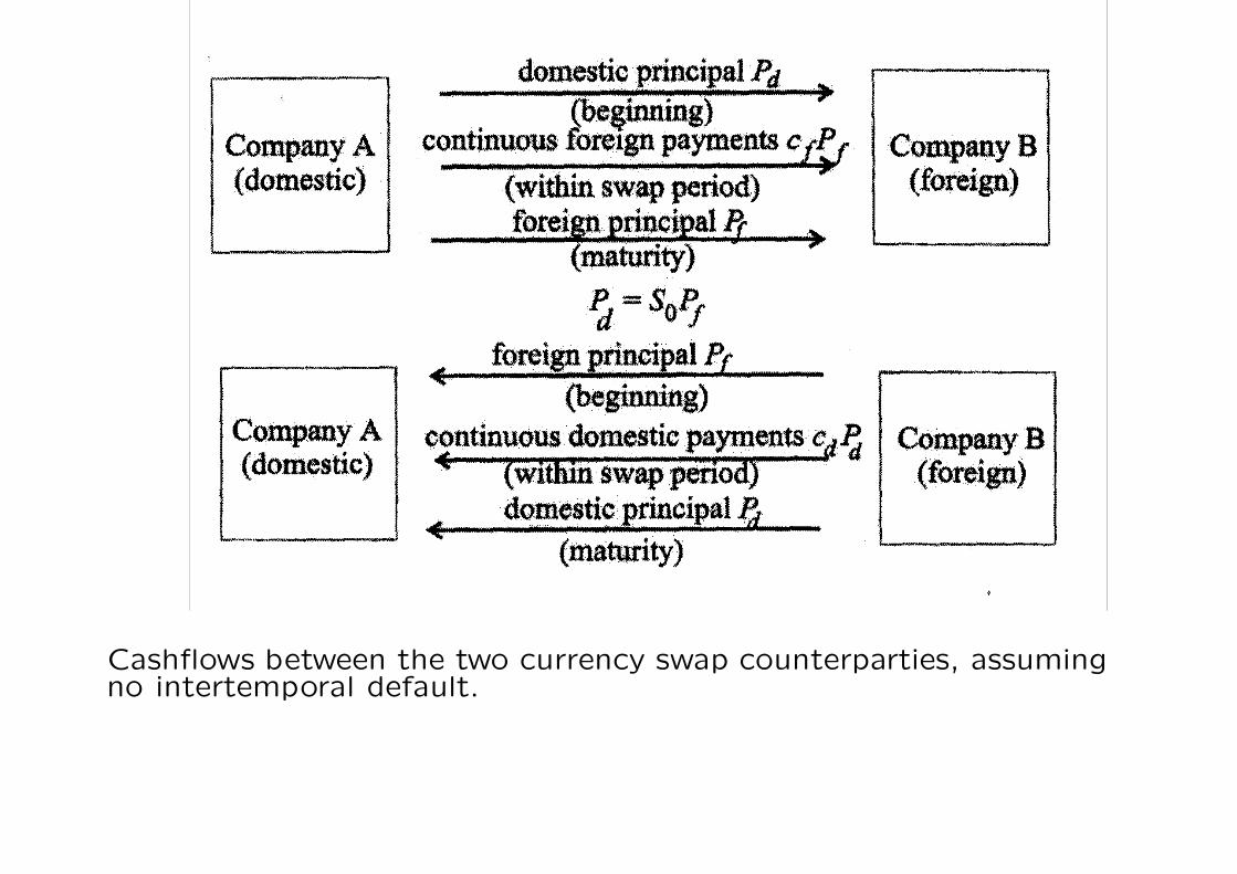
Cashflows between the two currency swap counterparties, assumingno intertemporal default.

Cashflows between currency swap counterparties

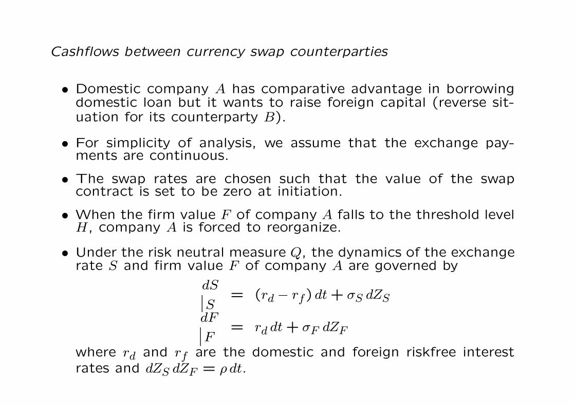
• Domestic company A has comparative advantage in borrowingdomestic loan but it wants to raise foreign capital (reverse sit-uation for its counterparty B).

• For simplicity of analysis, we assume that the exchange pay-ments are continuous.

• The swap rates are chosen such that the value of the swapcontract is set to be zero at initiation.

• When the firm value F of company A falls to the threshold levelH, company A is forced to reorganize.

• Under the risk neutral measure Q, the dynamics of the exchangerate S and firm value F of company A are governed by

dS

S= (rd − rf) dt + σS dZS

dF

F= rd dt + σF dZF

where rd and rf are the domestic and foreign riskfree interestrates and dZS dZF = ρ dt.

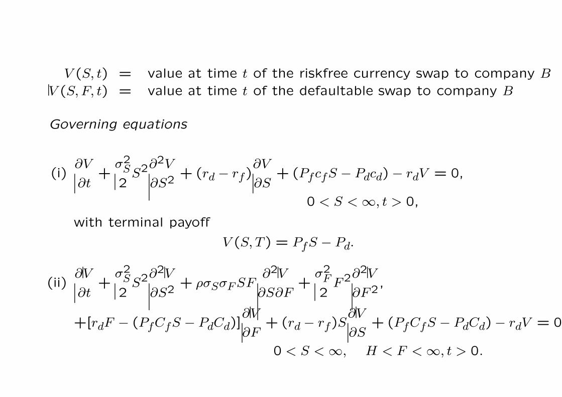
V (S, t) = value at time t of the riskfree currency swap to company B

V (S, F, t) = value at time t of the defaultable swap to company B

Governing equations

(i)∂V

∂t+

σ2S

2S2∂2V

∂S2+ (rd − rf)

∂V

∂S+ (PfcfS − Pdcd) − rdV = 0,

0 < S < ∞, t > 0,

with terminal payoff

V (S, T ) = PfS − Pd.

(ii)∂V

∂t+

σ2S

2S2∂2V

∂S2+ ρσSσF SF

∂2V

∂S∂F+

σ2F

2F2∂2V

∂F2,

+[rdF − (PfCfS − PdCd)]∂V

∂F+ (rd − rf)S

∂V

∂S+ (PfCfS − PdCd) − rdV = 0,

0 < S < ∞, H < F < ∞, t > 0.

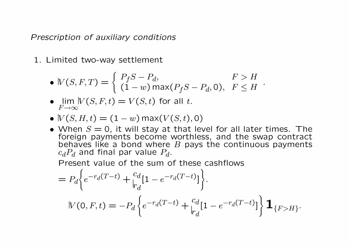
Prescription of auxiliary conditions

1. Limited two-way settlement

• V (S, F, T ) =

{PfS − Pd, F > H(1 − w)max(PfS − Pd,0), F ≤ H

.

• limF→∞

V (S, F, t) = V (S, t) for all t.

• V (S, H, t) = (1 − w)max(V (S, t),0)• When S = 0, it will stay at that level for all later times. The

foreign payments become worthless, and the swap contractbehaves like a bond where B pays the continuous paymentscdPd and final par value Pd.Present value of the sum of these cashflows

= Pd

{e−rd(T−t) +

cd

rd[1 − e−rd(T−t)]

}.

V (0, F, t) = −Pd

{e−rd(T−t) +

cd

rd[1 − e−rd(T−t)]

}1{F>H}.

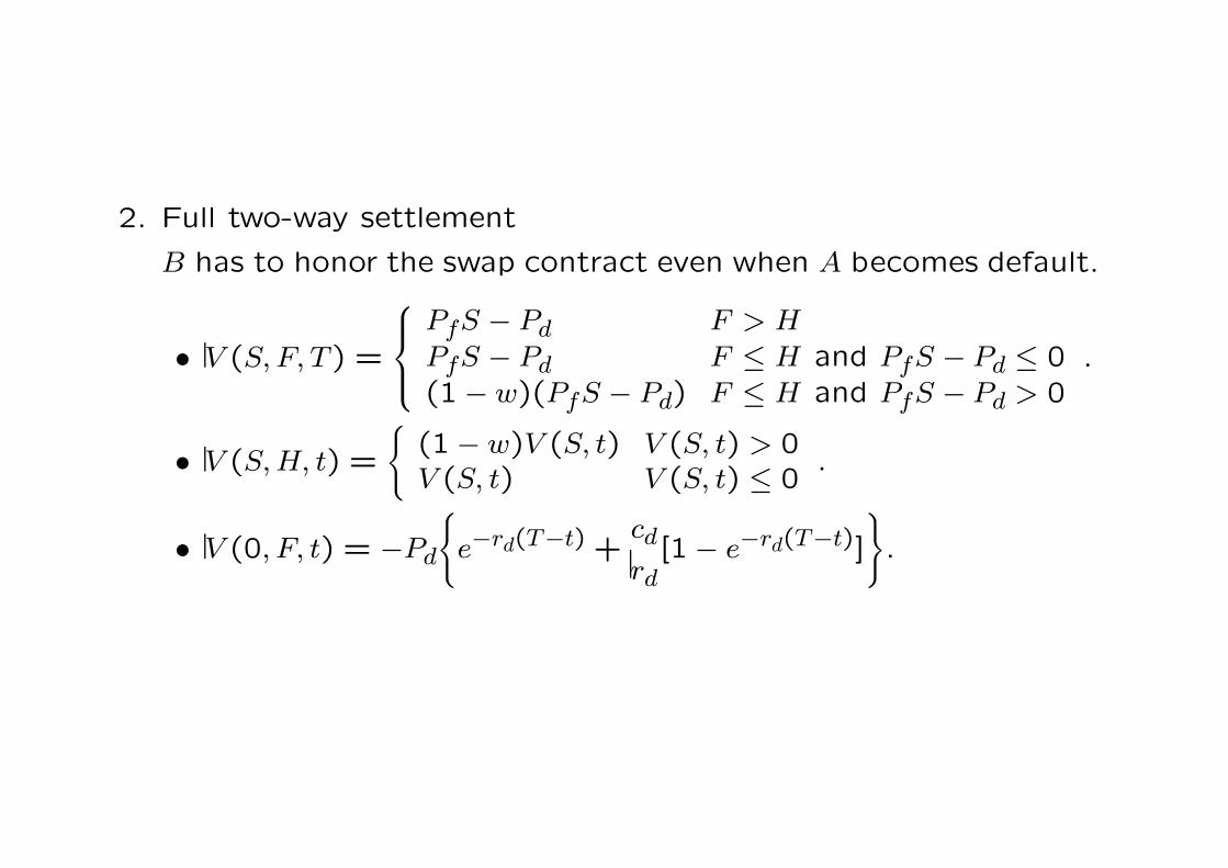
2. Full two-way settlement

B has to honor the swap contract even when A becomes default.

• V (S, F, T ) =

PfS − Pd F > H

PfS − Pd F ≤ H and PfS − Pd ≤ 0(1 − w)(PfS − Pd) F ≤ H and PfS − Pd > 0

.

• V (S, H, t) =

{(1 − w)V (S, t) V (S, t) > 0V (S, t) V (S, t) ≤ 0

.

• V (0, F, t) = −Pd

{e−rd(T−t) +

cd

rd[1 − e−rd(T−t)]

}.