POTENTIAL FIELD-BASED DECENTRALIZED CONTROL METHODS FORNETWORK CONNECTIVITY MAINTENANCE

By

ZHEN KAN

A DISSERTATION PRESENTED TO THE GRADUATE SCHOOLOF THE UNIVERSITY OF FLORIDA IN PARTIAL FULFILLMENT

OF THE REQUIREMENTS FOR THE DEGREE OFDOCTOR OF PHILOSOPHY

UNIVERSITY OF FLORIDA

2011

© 2011 Zhen Kan

2

To my wife Yang Chen, my mother Baozhi Hu, and my father Heping Kan, for their

unwavering support and constant encouragement

3

ACKNOWLEDGMENTS

I would like to express my deepest gratitude to my advisor, Warren E. Dixon, for his

guidance, patience and support in the completion of my Ph.D. As an advisor, he guided

me to start my graduate career on the right foot, encouraged me to explore my own ideas,

and helped me recover when my steps faltered. His experience helped me grow fast in the

four years of Ph.D study. I appreciate all his contributions of time, ideas and enthusiasm

to make my Ph.D experience productive and stimulating. In addition to help me mature

in the research, he also provided instrumental advices, like an elder brother or a close

friend, on my future career plan, job hunting, and other aspects of life. I feel so fortunate

to have had Dr. Dixon as my advisor, and I hope that one day I would become as good as

an advisor to my students as he has been to me.

I would like to extend my gratitude to my committee member, John Shea. I am

deeply grateful to him for the carefully reading and insightful comments on countless

revisions of my conference and journal publications, and constructive criticisms at different

stages of my research. I am also thankful to Prabir Barooah, and Carl D. Crane for

reading previous drafts of this dissertation and providing many valuable comments that

improved the presentation and contents of this dissertation.

I would also like to thank all the previous and current members of the NCR lab for

their various forms of support during my graduate study.

Last but not the least, I would like to thank my wife Yang. Without her support,

encouragement and unwavering love, I would never be able to finish my dissertation.

Also, I would like to thank my parents, who have been a constant source of love, concern,

support and strength all these years.

4

TABLE OF CONTENTS

page

ACKNOWLEDGMENTS . . . . . . . . . . . . . . . . . . . . . . . . . . . . . . . . . 4

LIST OF FIGURES . . . . . . . . . . . . . . . . . . . . . . . . . . . . . . . . . . . . 8

ABSTRACT . . . . . . . . . . . . . . . . . . . . . . . . . . . . . . . . . . . . . . . . 10

CHAPTER

1 INTRODUCTION . . . . . . . . . . . . . . . . . . . . . . . . . . . . . . . . . . 12

1.1 Motivation . . . . . . . . . . . . . . . . . . . . . . . . . . . . . . . . . . . . 121.2 Problem Statement . . . . . . . . . . . . . . . . . . . . . . . . . . . . . . . 131.3 Literature Review . . . . . . . . . . . . . . . . . . . . . . . . . . . . . . . . 141.4 Contributions . . . . . . . . . . . . . . . . . . . . . . . . . . . . . . . . . . 221.5 Dissertation Outline . . . . . . . . . . . . . . . . . . . . . . . . . . . . . . 27

2 VISION BASED CONNECTIVITY MAINTENANCE OF A NETWORK WITHSWITCHING TOPOLOGY . . . . . . . . . . . . . . . . . . . . . . . . . . . . . 29

2.1 Problem Formulation . . . . . . . . . . . . . . . . . . . . . . . . . . . . . . 292.1.1 Communication Graph . . . . . . . . . . . . . . . . . . . . . . . . . 302.1.2 Visibility Graph . . . . . . . . . . . . . . . . . . . . . . . . . . . . . 312.1.3 Connectivity Maintenance . . . . . . . . . . . . . . . . . . . . . . . 31

2.2 Control Strategy . . . . . . . . . . . . . . . . . . . . . . . . . . . . . . . . 322.3 Control Design . . . . . . . . . . . . . . . . . . . . . . . . . . . . . . . . . 35

2.3.1 Potential Field . . . . . . . . . . . . . . . . . . . . . . . . . . . . . . 352.3.2 Controller for Steady State . . . . . . . . . . . . . . . . . . . . . . . 372.3.3 Controller for Switching State . . . . . . . . . . . . . . . . . . . . . 37

2.4 Connectivity Analysis . . . . . . . . . . . . . . . . . . . . . . . . . . . . . 382.5 Simulation . . . . . . . . . . . . . . . . . . . . . . . . . . . . . . . . . . . . 402.6 Summary . . . . . . . . . . . . . . . . . . . . . . . . . . . . . . . . . . . . 40

3 NETWORK CONNECTIVITY PRESERVING FORMATION STABILIZA-TION AND OBSTACLE AVOIDANCE VIA A DECENTRALIZED CONTROLLER 43

3.1 Problem Formulation . . . . . . . . . . . . . . . . . . . . . . . . . . . . . . 433.2 Control Design . . . . . . . . . . . . . . . . . . . . . . . . . . . . . . . . . 453.3 Connectivity and Convergence Analysis . . . . . . . . . . . . . . . . . . . . 48

3.3.1 Connectivity Analysis . . . . . . . . . . . . . . . . . . . . . . . . . . 503.3.2 Convergence Analysis . . . . . . . . . . . . . . . . . . . . . . . . . . 52

3.4 Simulation . . . . . . . . . . . . . . . . . . . . . . . . . . . . . . . . . . . . 593.5 Summary . . . . . . . . . . . . . . . . . . . . . . . . . . . . . . . . . . . . 62

5

4 NETWORK CONNECTIVITY PRESERVING FORMATION RECONFIGU-RATION FOR IDENTICAL AGENTS FROM AN ARBITRARY CONNECTEDINITIAL GRAPH . . . . . . . . . . . . . . . . . . . . . . . . . . . . . . . . . . 63

4.1 Problem Formulation . . . . . . . . . . . . . . . . . . . . . . . . . . . . . . 644.2 Formation Reorganization Strategy . . . . . . . . . . . . . . . . . . . . . . 664.3 Network Topology Labeling Algorithms . . . . . . . . . . . . . . . . . . . . 67

4.3.1 Basic Algorithm . . . . . . . . . . . . . . . . . . . . . . . . . . . . . 674.3.2 Relabeling Algorithm . . . . . . . . . . . . . . . . . . . . . . . . . . 70

4.3.2.1 Branch Relabeling (BR) Algorithm . . . . . . . . . . . . . 724.3.2.2 Neighbor Relabeling (NR) Algorithm . . . . . . . . . . . . 73

4.4 Control Design . . . . . . . . . . . . . . . . . . . . . . . . . . . . . . . . . 744.4.1 Information Flow . . . . . . . . . . . . . . . . . . . . . . . . . . . . 744.4.2 Navigation Function-Based Control Scheme . . . . . . . . . . . . . . 774.4.3 Connectivity and Convergence Analysis . . . . . . . . . . . . . . . . 804.4.4 Convergence Analysis . . . . . . . . . . . . . . . . . . . . . . . . . . 81

4.5 Simulation . . . . . . . . . . . . . . . . . . . . . . . . . . . . . . . . . . . . 844.6 Summary . . . . . . . . . . . . . . . . . . . . . . . . . . . . . . . . . . . . 84

5 ENSURING NETWORK CONNECTIVITY FOR NONHOLONOMIC ROBOTSDURING DECENTRALIZED RENDEZVOUS . . . . . . . . . . . . . . . . . . 87

5.1 Problem Formulation . . . . . . . . . . . . . . . . . . . . . . . . . . . . . . 875.2 Control Design . . . . . . . . . . . . . . . . . . . . . . . . . . . . . . . . . 89

5.2.1 Dipolar Navigation Function . . . . . . . . . . . . . . . . . . . . . . 895.2.2 Control Development . . . . . . . . . . . . . . . . . . . . . . . . . . 93

5.3 Connectivity and Convergence Analysis . . . . . . . . . . . . . . . . . . . . 955.3.1 Connectivity Analysis . . . . . . . . . . . . . . . . . . . . . . . . . . 955.3.2 Convergence Analysis . . . . . . . . . . . . . . . . . . . . . . . . . . 95

5.4 Simulation . . . . . . . . . . . . . . . . . . . . . . . . . . . . . . . . . . . . 985.5 Summary . . . . . . . . . . . . . . . . . . . . . . . . . . . . . . . . . . . . 99

6 INFLUENCING EMOTIONAL BEHAVIOR IN SOCIAL NETWORK . . . . . 102

6.1 Preliminaries . . . . . . . . . . . . . . . . . . . . . . . . . . . . . . . . . . 1036.1.1 Fractional Calculus . . . . . . . . . . . . . . . . . . . . . . . . . . . 1036.1.2 Graph Theory . . . . . . . . . . . . . . . . . . . . . . . . . . . . . . 105

6.2 Problem Formulation . . . . . . . . . . . . . . . . . . . . . . . . . . . . . . 1066.3 Control Design . . . . . . . . . . . . . . . . . . . . . . . . . . . . . . . . . 1096.4 Convergence Analysis and Social Bond Maintenance . . . . . . . . . . . . . 110

6.4.1 Social Bond Maintenance . . . . . . . . . . . . . . . . . . . . . . . . 1116.4.2 Convergence Analysis . . . . . . . . . . . . . . . . . . . . . . . . . . 111

6.5 Discussion . . . . . . . . . . . . . . . . . . . . . . . . . . . . . . . . . . . . 1146.6 Summary . . . . . . . . . . . . . . . . . . . . . . . . . . . . . . . . . . . . 115

6

7 CONCLUSION AND FUTURE WORK . . . . . . . . . . . . . . . . . . . . . . 117

7.1 Conclusion . . . . . . . . . . . . . . . . . . . . . . . . . . . . . . . . . . . . 1177.2 Future work . . . . . . . . . . . . . . . . . . . . . . . . . . . . . . . . . . . 119

REFERENCES . . . . . . . . . . . . . . . . . . . . . . . . . . . . . . . . . . . . . . . 122

BIOGRAPHICAL SKETCH . . . . . . . . . . . . . . . . . . . . . . . . . . . . . . . . 130

7

LIST OF FIGURES

Figure page

2-1 Model of visibility graph. . . . . . . . . . . . . . . . . . . . . . . . . . . . . . . . 32

2-2 Schematic topology of underlying network. . . . . . . . . . . . . . . . . . . . . . 33

2-3 Evolution of nodes during time interval of t ∈ (0, 120). . . . . . . . . . . . . . . 41

2-4 Evolution of nodes during time interval of t ∈ (121, 220). . . . . . . . . . . . . . 41

3-1 An example of the artificial potential field generated for a disk-shaped workspacewith destination at the origin and an obstacle located at [1, 1]T . . . . . . . . . . 48

3-2 A connected initial graph with desired neighborhood in the workspace with staticobstacles. . . . . . . . . . . . . . . . . . . . . . . . . . . . . . . . . . . . . . . . 60

3-3 The achieved final configuration. . . . . . . . . . . . . . . . . . . . . . . . . . . 61

3-4 The inter-node distance during the evolution . . . . . . . . . . . . . . . . . . . . 61

3-5 The plot of the Fiedler eigenvalue of the Laplacian matrix during the evolution.The circle indicates the Fiedler eigenvalue of the graph at each time instance. . 62

4-1 The small disk area with radius δ1 denotes the collision region and the outerring area denotes the escape regions for node i. The region in the sensing zoneapart from collision and escape regions denotes the free-motion region. . . . . . 65

4-2 The example of an initially connected and desired graph topology, where thenodes denote the agent, and the lines connecting two nodes denote the avail-able communication links. In Fig. 4-2 (a) and (b), the root is assigned the label0. The children of the root are then assigned the labels 01, 02, 03 and 01,02 in Fig. 4-2 (a) and (b) respectively. Other nodes such as 021, 022, 031and 011, 012, 021, 022 are labeled by following a similar procedure. . . . . . . 70

4-3 Fig (a) and (b) illustrates a graph before performing BR algorithm and afterperforming BR algorithm respectively, where the shaded nodes denote the extranodes, the solid lines indicate the required edges in the desired topology in Fig.4-2(b), and the dashed line indicate the available communication links but notrequired to maintain for the desired topology. . . . . . . . . . . . . . . . . . . . 73

4-4 Fig (a) and (b) illustrates a graph before performing NR algorithm and afterperforming NR algorithm respectively, where the shaded nodes denote the ex-tra nodes, the solid lines indicate the required edges in the desired topology inFig. 4-2 (b), and the dashed line indicate the available communication linksbut not required to maintain for the desired topology. . . . . . . . . . . . . . . . 75

8

4-5 The desired formation is characterized by a "letter A", where the nodes denotethe agent, and the lines connecting two nodes denote the available communi-cation links. Fig (a) shows the desired formation, while Fig (b) shows how Fig(a) is labeled by prefix using the proposed prefix labeling algorithm. . . . . . . . 85

4-6 Fig (a) shows a randomly generated connected initial graph, while Fig (b) showshow the initial graph is labeled by prefix. In Fig (b), the solid lines indicatethe desired neighborhood, and the marked node 011111 is identified as an extranode. . . . . . . . . . . . . . . . . . . . . . . . . . . . . . . . . . . . . . . . . . 85

4-7 The trajectories of all nodes to achieve the desired formation, with "*" denot-ing their initial positions and circles denoting their final positions. . . . . . . . 86

5-1 An example of a dipolar navigation function with workspace of Rw = 5, andthe destination located at the origin with a desired orientation θ∗ = 0. . . . . . . 91

5-2 The trajectory for each mobile robot with the arrow denoting its current orien-tation. . . . . . . . . . . . . . . . . . . . . . . . . . . . . . . . . . . . . . . . . 99

5-3 Plot of linear velocity and angular velocity for each mobile robot. . . . . . . . . 100

5-4 Plot of position and orientation error for each mobile robot. . . . . . . . . . . . 100

5-5 The evolution of inter-robot distance. . . . . . . . . . . . . . . . . . . . . . . . . 101

6-1 The Zachary’s karate club network in [1] is modeled by an undirected graph G,where the numbered vertex in the graph represents the members of the club,and solid line connecting two individuals denotes the established social bond(i.e., friendship) in the club. . . . . . . . . . . . . . . . . . . . . . . . . . . . . . 108

9

Abstract of Dissertation Presented to the Graduate Schoolof the University of Florida in Partial Fulfillment of theRequirements for the Degree of Doctor of Philosophy

POTENTIAL FIELD-BASED DECENTRALIZED CONTROL METHODS FORNETWORK CONNECTIVITY MAINTENANCE

By

Zhen Kan

December 2011

Chair: Warren E. DixonMajor: Mechanical Engineering

In cooperative control for a multi-agent system, agents coordinate and communicate

to achieve a collective goal (e.g., flocking, consensus, or pattern formation). As agents

move to perform a desired mission objective, ensuring the group remains close enough to

maintain wireless communication (i.e., the group does not partition) is a great challenge

in a decentralized control manner. The use of an artificial potential field is one approach

that has been widely used in path planning for multi-agent systems, where an attractive

potential is used to model the control objective and a repulsive potential is used to

prevent collisions among the agents and obstacles. The focus of this dissertation is to

develop potential field based decentralized controllers for a group of agents with limited

sensing and communication capabilities to perform required mission objectives while

preserving network connectivity.

A two level control framework is developed in Chapter 2 for connectivity maintenance

and cooperation of a multi-agent system. All agents are categorized as clusterheads or

regular nodes. A high level graph is composed of all clusterheads while a low level graph

is composed of all regular nodes. Artificial potential field based controllers are then

developed to maintain existing links connected in both low and high level graphs and

ensure that a group of agents switch from one connected configuration to another without

disconnecting the underlying network in process.

10

In Chapter 3, based on the navigation function formalism, a decentralized control

method is designed to enable a group of agents to achieve a desired global configuration

from a given connected initial graph with desired neighborhood between agents, while

maintaining global network connectivity and avoiding obstacles, using only local feed-

back and no radio communication between the agents for navigation. The initial graph

assumption in Chapter 3 is then eliminated in Chapter 4, where a novel strategy using a

prefix labeling and routing algorithm and a navigation function based control scheme is

developed to achieve a desired formation for a group of identical agents from an arbitrarily

connected initial graph.

A group of mobile robots with nonholonomic constraints are considered in Chapter 5.

A decentralized continuous time-varying controller based on a modified dipolar navigation

function is developed to reposition and reorient those mobile robots with nonholonomic

constraints to a common setpoint with a desired orientation while maintaining network

connectivity during the evolution, using only local sensing feedback from its one-hop

neighbors.

The work in Chapter 6 applies the control techniques developed in engineering to

investigate and influence emotions of people in a social network, where a distributed

controller for each individual is designed to achieve emotion synchronization for a group of

individuals in a social network (i.e., an agreement on the emotion states of all individuals).

Motivated by the non-local property of fractional-order systems, the emotional response

of individuals in the network are modeled by fractional-order dynamics whose states

depend on influences from social bonds. Encoding the control objective of emotion

synchronization and modeling the maintenance of social bonds as a constraint, a potential

function is developed to ensure asymptotic convergence of each emotion state to the

common equilibrium in the social network.

Chapter 7 concludes the dissertation by summarizing the work and discussing some

remaining open problems that required further investigation.

11

CHAPTER 1INTRODUCTION

1.1 Motivation

Multi-agent systems under cooperative control provide versatile platforms that have

the potential to be used in various commercial and military applications. For instance, a

list of “some of the main applications for cooperative control of multi-vehicle systems” is

provided in [2], which includes:

• Military Systems: Formation Flight, Cooperative Classification and Surveillance,

Cooperative Attack and Rendezvous, and Mixed Initiative Systems;

• Mobile Sensor Networks: Environmental Sampling and Distributed Aperture

Observing;

• Transportation Systems: Intelligent Highways and Air Traffic Control.

These types of tasks usually require or can benefit from collaborative motion of a group

of agents, and thus the agents must be able to exchange information over some form

of communications network. For most applications, communications will be over a

wireless network, in which the communication links between agents are dependent on the

propagation of electromagnetic signals between the agents, and the electromagnetic power

density decreases with distance. However, when performing desired tasks, the underlying

network connectivity can be impacted due to the motion of agents. If the network is

partitioned, the agents can no longer coordinate their movements, and the mission may

fail. Hence, control algorithms must be designed in a cooperative manner to preserve

network connectivity when performing desired tasks.

Some applications can adopt a centralized control approach where one algorithm

determines and communicates the next required movement for each agent. For some ap-

plications, the centralized approach is not practical due to the potential for compromised

communication with or demise/corruption of the central controller. Decentralized control

is an alternative approach in which each agent makes an independent decision based on

12

either global information communicated through the network or local information from

one-hop neighbors. Methods that use global information require each agent to determine

the relative trajectory of all other agents at all time by propagating information through

the network, resulting in delays in the trajectory information and consumption of network

bandwidth, effects that limit the network size. Methods that use local information need

only relative trajectories of neighboring agents; however, difficulties arising from perform-

ing required mission objectives for the global network using local feedback can cause the

network to partition. When the network partitions, communication between groups of

agents can be permanently severed leading to mission failure.

Given the wide application of multi-agent systems and the desire to maintain network

connectivity in a decentralized manner, this dissertation is motivated by the following

questions:

1. How can a decentralized control strategy be designed to ensure global network

connectivity using only local available information?

2. How can the required collective mission objective be achieved in a cooperative way

while preserving network connectivity?

3. Is it possible to extend the models and methods developed for multi-agent systems

in engineering be leveraged to yield insight to influence social groups?

1.2 Problem Statement

Accomplishing desired collective mission objectives for a networked multi-agent

system highly depends on the coordination of their actions and the peer-to-peer, wireless

communication among agents. In this dissertation, limited communication and sensing

capabilities for each agent are considered, that is two agents can communicate and

exchange information if they are within a specified maximum communication range and

cannot communicate if they are outside of that range. Hence, ensuring that the overall

network remains connected requires the specified agents stay within predetermined sensing

and communication ranges, and the cooperative objectives must be accomplished by using

13

local information obtained from the limited sensing and communication abilities of each

agent. The work presented in this dissertation examines decentralized control methods for

networked multi-agent systems to achieve global collective objectives, such as formation

control and consensus, while preserving connectivity of the global network using local

information from immediate neighbors.

1.3 Literature Review

This section provides a review of relevant literature for each chapter.

Maintenance of network connectivity for a multi-agent system: Motivated

by the practical need to keep agents in a single group, recent results such as [3–11] are

focused on the network connectivity maintenance problem based on the construction of

an artificial potential field. Artificial potential fields are have been widely used in path

planning for multi-agent systems, where an attractive potential is used to model the

control objective and a repulsive potential is used to prevent collisions among the agents

and obstacles [12, 13]. In [3] and [10], a potential field based centralized control approach

is developed to ensure the connectivity of a group of agents using the graph Laplacian

matrix. However, global information of the underlying graph is required to compute

the graph Laplacian. In [4], connectivity maintenance is performed in the discrete space

of graphs to verify link deletions with respect to connectivity, and motion control is

performed in the continuous configuration space using a potential field. In [5], a potential

field-based neighbor control law is designed to achieve velocity alignment and network

connectivity among different topologies. In [6] and [8], a repulsive potential is used for

a collision avoidance objective, and an attractive potential field is used to drive agents

together. Distributed control laws are investigated to ensure edge maintenance in [11]

by allowing unbounded potential force whenever pairs of agents are about to break the

existing links.

To ensure network connectivity during the mission, a two level control strategy is

developed for a multi-agent system in Chapter 2, where all agents are categorized as

14

clusterheads or regular nodes. A high level graph is composed of all clusterheads and the

motion of the clusterheads is controlled to maintain existing connections among them.

A low level graph composed of all regular nodes is controlled to maintain connectivity

with respect its specific clusterhead. Artificial potential field based controllers are then

developed in Chapter 2 to maintain the existing links connected in both low and high

level graphs all the time and to ensure that a group of agents switch from one connected

configuration to another without disconnecting the network.

Formation control with network connectivity for a multi-agent system:

Typical approaches in formation control include leader-follower [14, 15], behavioral-

based [16, 17], virtual structures [18, 19] and graph-theory-based [10, 20–25] methods,

to name a few. However, no constraints on the availability of other agents’ states and

information about the environment are considered: network connectivity is not taken into

account in such results. When considering network connectivity, overviews of techniques

for formation control are given in [2, 26, 27]. The earliest works on formation control

with network connectivity are discussed in [26] with a focus on the impact of a given

network connectivity on the stability and controllability of formations of robots without

considering the control required to ensure network connectivity during the mission.

Although some results described in [2, 27] are focused on maintaining network connectivity

during formation control, an open problem remains in developing design a decentralized

control approach for a group of agents seeking a desired formation in an uncertain

environment while preserving network connectivity.

One of the most widely used approaches in formation control is to use artificial

potential fields to guide the movement of the agents. A common problem with artificial

potential field-based control algorithms is the existence of local minima when attractive

and repulsive force are combined [28]. In Chapter 2, network connectivity is ensured by

using an artificial potential field-based controller; however, the agents have the potential

to be trapped by local minima. A specific type of artificial potential, called a navigation

15

function, achieves a unique minimum (c.f., [29–31]) and has been widely used in motion

control for multi-agent systems (see e.g., [4, 32–35]). The navigation function developed

in [30] is a real-valued function that is designed so that the negated gradient field does

not have a local minima. The negated gradient of the navigation function is attracted

towards the goal and repulsed by obstacles for almost all initial states. As such, closed-

loop navigation function approaches guarantee convergence to a desired destination. The

navigation function framework is extended to multi-agent systems for obstacle avoidance

in results such as [28, 34, 36–38]; however, agents within these results acted independently

and were not required to achieve a network objective. In contrast, results in [39–41]

use potential fields/navigation functions to achieve obstacle avoidance while the agents

are also required to achieve a cooperative network objective (e.g., formation control or

consensus); however, these results assume the agents can always communicate (i.e., the

graph nodes are assumed to remain connected). The assumption of a connected graph is

restrictive for a mobile network, where communication depends on the distance between

agents, which can also be a function of the environment and available transmitting power.

In [9], a potential field is designed for a group of mobile agents to perform desired tasks

while maintaining network connectivity. It is unclear how the potential field method in [9]

can be extended to include static obstacles, since the resulting closed-loop dynamics can

not be expressed as a Metzler matrix with zero sums as required in the analysis in [9].

Moreover, the work in [9] only proves that all states converge to a common value that can

be influenced by the initial states [42].

Motivated to avoid local minima when using artificial potential field-based approach,

a navigation function based decentralized controller is developed in Chapter 3 to ensure

network connectivity and stabilize a group of agents in a required formation from a

connected initial graph (agents are considered as nodes on a graph) with a desired

neighborhood, while avoiding collisions with other agents and external obstacles.

16

Formation control with network connectivity from an arbitrary initial

graph: The result in Chapter 3 requires that the initial graph is connected in a desired

way so that no initial communication link is allowed to be broken during the motion.

Similar constraints on the initial graph connections are also presented in works such as [9]

and [35]. However, assumptions on the initial graph can be limiting, since some applica-

tions may require agents to achieve desired formations from an arbitrary initial graph or

dynamically change the achieved formations to adapt to the uncertain environment. For

example, certain formations have proven to be particularly advantageous for efficiency of

data gathering, data processing, and forecasting (cf., [43, 44]). Since the initial topology or

the topology from the previous task may not be conducive to the current task, achieving

a desired formation or transforming from one topology to another for a group of agents

with limited knowledge is a challenging task. Hence, maintaining the overall network

connectivity is paramount, and stabilizing a multi-agent system at a desired formation

from an arbitrary initial topology using local feedback can be challenging.

In Chapter 4, each agent possesses only limited knowledge (i.e., limited sensing

capabilities or knowledge about the environment and limited communication capabilities

with nearby agents) to perform tasks such as formation control in a cooperative manner,

where agents are required to coordinate their motion with respect to other agents.

Limited sensing capabilities by agents in a network has been examined in results such

as [39,41,45–47]. In [45], assuming that each agent is aware of its own destination, a group

of mobile agents with limited sensing range is controlled to achieve desired formations

based on a potential-field based approach in a non-cooperative way, where agents are not

required to coordinate their motion with respect to other agents to achieve the desired

formation. The result in [45] is extended to perform formation tracking in a cooperative

way in [46], where limited sensing is used for collision avoidance only. A centralized leader-

follower approach is developed to perform formation tracking in [47], and a centralized

navigation function-based control strategy is developed in [39] to steer a group of mobile

17

agents with limited sensing capabilities to achieve a desired formation. Motivated by the

need to maintain network connectivity, an artificial potential field-based decentralized

method is used to prevent the network from partitioning and stabilize a group of agents

with limited communication and sensing capabilities in a desired formation in [9, 11, 48],

where the network connectivity is guaranteed by maintaining the initially established

neighborhood all the time during the operation. However, a common assumption in the

results of [9, 11, 48] is that the initial topology is required to be a supergraph of the desired

topology ensuring the agents are originally in a feasible interconnected state. Such results

may not be applicable to the applications which require a multi-agent system to start from

an arbitrary connected initial graph or dynamically change the achieved formations to

adapt to the uncertain environment, since the reorganization of the initial topology to a

desired one may require the breakage of some prespecified neighborhood and results in the

partition of the underlying network connectivity.

Contrary to the work of [9, 39, 41, 45–48], formation control for a group of agents

with limited sensing and communication capabilities are considered in Chapter 4, in

which the agents are identical and can take any position in the final topology. Based on

the concepts of prefix labeling and prefix routing in [49–51], a novel network topology

labeling algorithm developed in our previous work [52] is modified to dynamically specify

the neighborhood of each agent in the initial graph according to the desired formation,

and determine the required movement for all nodes to achieve the desired formation. By

modeling network connectivity as an artificial obstacle, a navigation function based control

scheme is developed in Chapter 4 to guarantee network connectivity by maintaining the

neighborhood among agents determined by the prefix labeling algorithm, and ensure the

convergence of all agents to the desired configuration with collision avoidance among

agents using local information (i.e., local sensing and communication). An information

flow is then proposed from the work of [53] and [54] to specify the required movement for

extra agents to their destination nodes. The information flow-based approach generally

18

provides a path with more freedom for the motion of extra nodes without partitioning the

network connectivity and allows communication links to be formed or broken in a smooth

manner without introducing discontinuity. Convergence is proven using Rantzer’s Dual

Lyapunov Theorem [55].

Rendezvous of wheeled mobile robots with network connectivity: Results

such as [3–11] are developed to maintain the network connectivity in the application of

formation control, flocking, consensus and other tasks in either centralized or decentralized

manner. However, one common feature in most of the aforementioned work is that only

linear models of motion are taken into account, i.e., the first order integrator. Although

control design for the stabilization of a single robot with nonholonomic constraints has

been extensively studied in the past decades [56, 57], such controllers may not be appli-

cable for a networked multi-robot system with a cooperative objective, e.g., maintaining

network connectivity. Motivated to navigate a system with nonholonomic constraints to

a destination with a desired orientation, a dipolar navigation function was proposed and

a discontinuous time-invariant controller was developed to navigate a single robot in [58].

The work in [58] was then extended to a multi-robot system with both holonomic and

nonholonomic constraints in [36] and extended to navigate a nonholonomic system in three

dimensions in [59]. However, only a time-invariant discontinuous controller was developed

in [36, 58, 59]. In [8], when considering maintenance of the network connectivity, based

on the work of [58], a discontinuous controller was used to steer a multi-robot system

with nonholonomic constraints to rendezvous at a common position. However, each robot

can only achieve the destination with arbitrary orientation and has to reorient at the

destination. Moreover, the multi-robot system can only converge to a destination which

depends on the initial deployment in [8]. Based on our previous work in [60], a decentral-

ized continuous time-varying controller, using only local sensing feedback from its one-hop

neighbors, is designed in Chapter 5 to stabilize a group of wheeled mobile robots with

19

nonholonomic constraints at a specified common setpoint with a desired orientation, while

maintaining network connectivity during network regulation.

Consensus of human emotion in a social network: Social interactions influence

our thoughts and actions through social networks which provide a means for more

rapid, convenient, and widespread communication. For instance, flash mobs are being

organized through social media for events ranging from entertaining public spontaneity to

vandalism, violence, and crime [61–63]. Recent riots and protests [64–67] and ultimately

revolution [68, 69], have been facilitated through social media technologies such as

Facebook, Twitter, You Tube, and BlackBerry Messaging (BBM). In attempts to prevent,

mitigate, or prosecute the sources of such social unrest, governments and law enforcement

agencies are placing a greater emphasis on examining (and ultimately controlling) the

structure of social networks. Scotland Yard is looking to social media websites as part

of investigations into widespread looting and rioting in London [66, 67], and police in

San Francisco disabled access to social networks by cutting off cellphone service as a

means to prevent riots due to a police shooting [65]. One U.S. Intelligence strategy in

Afghanistan is to focus on answering rudimentary questions about Afghanistan’s social

and cultural fabric through tools such as Nexus 7 to tap into the exabytes of information

“for leveraging popular support and marginalizing the insurgency” [70]. Yet other’s argue

that Nexus 7 lacks models or algorithms.

Models and algorithms have been extensively developed for various engineered

networks and multi-agent systems [2]. Consensus is a particular class of network control

problem that has been extensively studied where the goal is for the individual nodes to

reach an agreement on the states of all agents [71–73]. However, an interesting question

that has received little attention is how can such models and methods be applied toward

understanding and controlling a social network. How can one produce consensus among a

social network (e.g., to manipulate social groups to a desired end)? Motivated towards this

20

end, the focus of Chapter 6 is to influence the emotions of a socially connected group of

individuals to a consensus state.

Various dynamic models have been developed for psychological phenomena, including

efforts to model the emotional response of different individuals [74–76]. A dynamic model

of love is reported in the work of [74], which describes the time-variation of the emotions

displayed by individuals involved in a romantic relationship. In [75], happiness is modeled

by a set of differential equations, and the time evolution of one’s happiness in response to

external inputs is examined. A mathematical model of fear is also described in the work

of [76].

Fractional-order differential equations are a generalization of integer-order differential

equations which exhibit a non-local property where the next state of a system not only

depends upon its current state but also upon its historical states starting from the initial

time [77]. This property has motivated researchers to explore the use of fractional-order

systems as a model for various phenomena in natural and engineered systems, and in

relation to the current context, have also been explored as a potentially more appropriate

model of psychological behavior. For example, the integer-order dynamic models of love

and happiness developed in [74] and [75] were revisited in [78] and [79], where the models

were generalized to fractional-order dynamics, since a person’s emotional response is

influenced by past experiences and memories. However, the results in [74, 75, 78, 79] focus

on an individual’s emotion model, without considering the interaction among individuals

in the context of a social network where rapid and widespread influences from the social

peers can prevail.

Instead of studying an individual model of a person’s emotional response, Chapter 6

develops an approach to influence the interaction of a person’s emotions within a social

network. Motivated by the non-local property of fractional-order systems, the emotional

response of individuals in the network are modeled by fractional-order dynamics whose

states depend on influences from social bonds. Within this formulation, the social group

21

is modeled as a networked fractional system. The first apparent result that investigated

the coordination of networked fractional systems is [80], in which linear time invariant

systems are considered and where the interaction between agents is modeled as a link with

a constant weight. In this chapter, the social bond between two persons is considered as

a weight for the associated edge in the graph measuring the closeness of the relationship

between the individuals. In comparison to [80], the main challenge in this work is that

social bonds are time varying parameters which depends on the emotional states of

individuals. Previous stability analysis tools such as examining the Eigenvalues of linear

systems for fractional-order systems (cf. [79–81]) are not applicable to the time-varying

system in Chapter 6. To achieve these objectives of maintaining existing social bonds

among individuals (i.e., social controls or influences should not be so aggressive that they

isolate or break bonds between people in the social group) and emotion synchronization

in the social network (i.e., an agreement on the emotion states of all individuals), a

decentralized potential function is developed in Chapter 6, and asymptotic convergence of

each emotion state to the common equilibrium in the social network is then analyzed via a

Metzler Matrix [42] and a Mittag-Leffler stability [82] approach.

1.4 Contributions

The contributions of Chapters 2-6 are discussed as follows:

1. Vision Based Connectivity Maintenance of a Network with Switching

Topology: The main contribution in Chapter 2 is the development of a two level

control framework for connectivity maintenance and cooperation of multi-agent

systems. Each agent is equipped with an omnidirectional camera and wireless

communication capabilities, which indicates that each agent is able to see the

other agents within its field of view and can communicate with other agents within

its communication zone to exchange information. Motivated to reduce the use of

interagent radio communication for the maintenance of network connectivity, a two

level graph is developed, where all agents are categorized as either clusterheads or

22

regular nodes. A high level graph is composed of all clusterheads and the motion

of the clusterheads is controlled to maintain existing connections among them. A

low level graph composed of all regular nodes is controlled to maintain connectivity

with respect its specific clusterhead. Image feedback is used as the primary method

to maintain connectivity among agents while wireless communication is only used

to broadcast information when a specific topology change occurs. One benefit of

using image feedback as a primary tool is that radio communication may not be

applicable in some dynamic, hostile, or tactical environments, and even when radio

communication is possible the network bandwidth may be required for distributing

other data. Another contribution of this work is the development of the artificial

potential field based controllers to maintain the existing links connected in both

low and high level graph all the time, and to ensure that a group of agents switches

from one connected configuration to another without disconnecting the network in

process.

2. Network Connectivity Preserving Formation Stabilization and Obstacle

Avoidance via A Decentralized Controller: decentralized control method

is developed in Chapter 3 to enable a group of agents to achieve a desired global

configuration while maintaining global network connectivity and avoiding obstacles,

using only local feedback and no radio communication between the agents for nav-

igation. Each agent is equipped with a range sensor (e.g., camera) to provide local

feedback of the relative trajectory of other agents within a limited sensing region,

and a transceiver to broadcast information to immediate neighbors. By modeling the

interaction among the agents as a graph, and given a connected initial graph with

desired neighborhood between agents, the developed method achieves convergence

to a desired configuration and maintenance of network connectivity using a decen-

tralized navigation function approach which uses only local feedback information.

By using a local range sensor (and not requiring knowledge of the complete network

23

structure as in methods that use a graph Laplacian), an advantageous feature of the

developed decentralized controller is that no inter-agent communication is required

(i.e., communication free global decentralized group behavior). That is, connectivity

is maintained so that radio communication is available when required for various

task/mission scenarios, but communication is not required to navigate, enabling

stealth modes of operation. Collision avoidance and network connectivity are em-

bedded as constraints in the navigation function. By proving that the distributed

control scheme is a valid navigation function, the multi-agent system is guaranteed

to converge to and stabilize the desired configuration.

3. Network Connectivity Preserving Formation Reconfiguration for Identical

Agents From An Arbitrary Connected Initial Graph: Achieving a desired

formation for a group of identical agents with limited sensing and communication

capabilities from an arbitrarily connected initial graph is considered in Chapter

4. The local interaction among agents is modeled by a dynamic graph and the

goal is to achieve a desired formation which is characterized by a given inter-agent

distance from an arbitrary connected initial graph while maintaining network

connectivity in a decentralized manner. Contrary to the limitation in most existing

work in formation control (cf. [2, 26, 27] and their references) where the absolute or

relative poses of the agents are prespecified, and the initial topology requires to be a

supergraph of the desired topology, a novel formation control technique is developed

in Chapter 4, in which the robots are identical and can take any position in the final

topology. That is, we do not wish to specify which nodes in the initial topology will

take which positions in the final topology; rather, we only care that there is an agent

in each position specified in the final topology. Assuming that the final topology is

a tree, a prefix labeling and routing algorithm from [52] is modified to specify the

neighborhood of each agent according to the desired formation allowing the agents

to interchange their roles, and determine the required movement for all nodes to

24

achieve the desired formation. By modeling the network connectivity as an artificial

obstacle, a navigation function based control scheme is developed in this chapter

to guarantee the network connectivity by maintaining the neighborhood among

agents determined by the prefix labeling algorithm, and ensure the convergence of

all agents to the desired configuration with collision avoidance among agents using

local information (i.e., local sensing and communication). An information flow is

then proposed from the work of [53] and [54] to specify the required movement

for extra agents to their destination nodes. The information flow-based approach

generally provides a path with more freedom for the motion of extra nodes without

partitioning the network connectivity and allows communication links to be formed

or broken in a smooth manner without introducing discontinuity. Convergence is

proven using Rantzer’s Dual Lyapunov Theorem [55].

4. Ensuring Network Connectivity for Nonholonomic Robots During De-

centralized Rendezvous: Assuming a range sensor (e.g., camera) provides local

feedback of the relative trajectory of other robots within a limited sensing region

and a transceiver is used to broadcast information to immediate neighbors on each

robot, the objective in Chapter 5 is to reposition and reorient a group of wheeled

robots with nonholonomic constraints to a common setpoint with a desired orienta-

tion while maintaining network connectivity during the evolution. A distinguishing

feature of this work is that it also considers a cooperative objective of maintaining

the network connectivity during network regulation for a group of mobile robots.

Another feature of the developed decentralized controller is that, using local sensing

information, no inter-agent communication is required (i.e., communication-free

global decentralized group behavior). That is, network connectivity is maintained

so that the radio communication is available when required for various tasks, but

communication is not required for regulation. Using a dipolar navigation function

framework, the multi-robot system is guaranteed to maintain connectivity and be

25

stabilized at a common destination with a desired orientation without being trapped

by local minima. Moreover, the result can be extended to other applications by

replacing the objective function in the navigation function to accommodate different

tasks, such as formation control, flocking, and other applications.

5. Influencing Emotional Behavior in Social Network: Instead of studying net-

worked control problems in engineering as in Chapter 2-5, Chapter 6 investigates an

approach to influence the interaction of a person’s emotions within a social network.

Using graph theory, a social network is modeled as an undirected graph, where an

individual in the social network is represented as a vertex in the graph, and the

social relationship between two individuals is represented as an edge connecting

two vertices. The social bond between two persons is considered as a weight for the

associated edge in the graph measuring the closeness of the relationship between

the individuals. Motivated by the non-local property of fractional-order systems,

where the next state of a system not only depends upon its current state but also

upon its historical states starting from the initial time, the emotional response of

individuals in a social network is modeled by fractional-order dynamics whose states

depend on influences from social bonds. Within this formulation, the social group is

modeled as a networked fractional system. Contrary to the first apparent result that

investigated the coordination of networked fractional systems in [80], in which linear

time invariant systems are considered and where the interaction between agents is

modeled as a link with a constant weight, the main feature in this chapter is that

social bonds are time varying parameters which depends on the emotional states of

individuals. Previous stability analysis tools such as examining the Eigenvalues of

linear systems for fractional-order systems (cf. [79–81]) are no longer applicable to

the time-varying system in this chapter. This chapter also considers a social bond

threshold on the ability of two people to influence each other’s emotions. To ensure

interaction among individuals, one objective is to maintain existing social bonds

26

among individuals above the prespecified threshold all the time (i.e., social controls

or influences should not be so aggressive that they isolate or break bonds between

people in the social group). Another objective is to design a distributed controller

for each individual, using local emotional states from social neighbors, to achieve

emotion synchronization in the social network (i.e., an agreement on the emotion

states of all individuals). To achieve these objectives, a decentralized potential func-

tion is developed to encode the control objective of emotion synchronization, where

maintenance of social bonds is modeled as a constraint embedded in the potential

function. Asymptotic convergence of each emotion state to the common equilibrium

in the social network is then analyzed via a Metzler Matrix [42] and a Mittag-Leffler

stability [82] approach.

1.5 Dissertation Outline

Chapter 1 serves as an introduction, where the motivation, problem statement,

literature review and the contributions of the dissertation are discussed.

Chapter 2 describes a two level control framework for connectivity maintenance

and cooperation of multi-agent systems. Artificial potential field based controllers are

developed to maintain existing links connected in both low and high level graphs all the

time, and also ensure that a group of agents switches from one connected configuration to

another without disconnecting the network in process.

Chapter 3 provides a decentralized control method based on the navigation function

formalism to enable a group of agents to achieve a desired global configuration from a

connected initial graph with desired neighborhood between agents, while maintaining

global network connectivity and avoiding obstacles, using only local feedback and no radio

communication between the agents for navigation. The performance of the decentralized

control method is illustrated through simulations.

Chapter 4 illustrates a novel formation control strategy for a group of identical agents

with limited sensing and communication capabilities to achieve a desired formation from

27

an arbitrarily connected initial condition. A prefix labeling and routing algorithm is

modified to specify the neighborhood of each agent according to the desired formation

allowing the agents to interchange their roles, and determine the required movement for

all nodes to achieve the desired formation. A navigation function based control scheme

is developed to guarantee the network connectivity by maintaining the neighborhood

among agents determined by the prefix labeling algorithm, and ensure the convergence of

all agents to the desired configuration with collision avoidance among agents using local

information (i.e., local sensing and communication). Simulation results are provided to

illustrate the developed strategy.

Chapter 5 develops a dipolar navigation function and corresponding time-varying con-

tinuous controller to reposition and reorient a group of wheeled robots with nonholonomic

constraints, while maintaining the network connectivity during the mission, by using only

local sensing feedback information from neighbors. Simulation results demonstrate the

performance of the developed approach.

Chapter 6 extends the approaches developed in previous chapters to provide a means

to influence the human emotion for a group of individual in a social network. The social

interactions among individuals in a social network are modeled as an undirected graph

with each vertex representing an individual and each edge representing a social bond

between individuals. By modeling the emotional response of individuals in the network

as fractional-order dynamics whose states depend on influences from social bonds, a

decentralized control method is developed to manipulate the social group to a common

emotional state while maintaining existing social bonds (i.e., without isolating peers in the

group). Asymptotic convergence to a common equilibrium point (i.e., emotional state) of

the networked fractional-order system is proved by using Mittag-Leffler stability.

Chapter 7 concludes the dissertation by summarizing the work and discussing some

remaining open problems that require further investigation.

28

CHAPTER 2VISION BASED CONNECTIVITY MAINTENANCE OF A NETWORK WITH

SWITCHING TOPOLOGY

In most applications of a multi-agent system, agents need to coordinate and com-

municate to take appropriate decisions to fulfill a pre-specified goal. In this chapter, each

robot is assumed to be equipped with an omnidirectional camera that can measure the

relative position of the other agents in its sensing area, and some form of transceiver that

can be used to broadcast information to local nodes. Two moving agents can communicate

with each other if they remain within a specific distance. As agents move to perform some

mission objective, it is paramount to ensure that the group of agents remain connected

(i.e., the group does not partition). Motivated to reduce interagent radio communication,

a network connectivity maintenance objective is considered in this chapter that relies

primarily on image feedback. A two level control strategy is developed in [83], where all

agents in the team are categorized as clusterheads or regular nodes. A high level graph is

composed of all clusterheads and the motion of the clusterheads is controlled to maintain

existing connections among them. A low level graph composed of all regular nodes is

controlled to maintain connectivity with respect its specific clusterhead. Connectivity

of the network is maintained using image feedback only unless a clusterhead change is

required. If the clusterhead changes and the network needs to reorganize the topology,

only then is the wireless communication used to alert the nodes of the topology change.

Artificial potential field based controllers are then developed to maintain the existing links

connected in both low and high level graphs all the time and to ensure that a group of

agents switches from one connected configuration to another without disconnecting the

network in process.

2.1 Problem Formulation

Consider a network composed of N agents, where agent i moves according to the

following kinematics:

xi(t) = ui(t), i ∈ V = 1, . . . , N (2–1)

29

where xi(t) ∈ R2 denotes the position of agent i in a two dimensional (2D) plane at time

t, and x(t) ∈ R2N denotes the stack position vectors of all agents. In (2–1), ui(t) ∈ R2

denotes the velocity of agent i (i.e. the control input). The interaction of the group is

modeled as a dynamic graph, in the sense that it evolves in time with its connectivity

governed by the kinematics of the agents (2–1). This time varying property gives rise to

the notion of a dynamic graph, G(t) = (V , E(t)), in which the set of links E(t) is time

varying and each component in V stands for the index of an agent. Given the assumption

that each agent is equipped with an omnidirectional camera and wireless communication

capabilities, two different graph models need to be specified: a communication graph

and a visibility graph. Each graph is composed of different types of nodes: clusterheads

and regular nodes, and the interaction between the nodes in each graph is modeled in a

different way.

2.1.1 Communication Graph

Inter-agent communication is modeled in terms of a time-varying communication

graph Gc = (V , Ec(t)) with the index set of nodes V and set of edges

Ec(t) = (i, j) ∈ V × V| ‖xij‖ ≤ Rc . (2–2)

In (2–2), each node is located at a position xi, ‖xij‖ ∈ R+ is defined as

‖xij‖ = ‖xi − xj‖ , (2–3)

and Rc denotes the maximum communication radius. The communication graph Gc

is an undirected graph in the sense that nodes i can influence node j and vice versa.

An undirected communication link between nodes i and j is denoted by (i, j) when

‖xij‖ ≤ Rc. The index set of neighbors of node i is denoted by

N ci = j : j 6= i|j ∈ V , (i, j) ∈ Ec .

30

2.1.2 Visibility Graph

Each agent is capable of sensing a disk area with the maximum radius Rv ≤ Rc, so

that any two agents are able to communicate with each other as long as they can see each

other. The visibility graph is modeled as a undirected time-varying graph Gv = (V , εv(t))

with the index set of nodes V and set of edges

εv = (i, j) ∈ V × V| ‖xij‖ ≤ Rv .

For the visibility graph, the edge (i, j) is undirected indicating that, if node i can see

node j, node j can also see node i. The index set of neighbors of node i is denoted

by N vi = j : j 6= i|j ∈ V , (i, j) ∈ Ev(t) . The subsequent development is based on

the assumption that the distance between two nodes can be estimated from the image

feedback (e.g., using methods as in [84]).

2.1.3 Connectivity Maintenance

Since Rv ≤ Rc, a sufficient goal to ensure Gc remains connected is to ensure the

visibility graph Gv remains connected. For simplicity, the following development is

based on the assumption that Rv = Rc = R without loss of generality. To understand

connectivity for each graph, consider Fig 2-1. For the communication graph, if node i

in Fig 2-1 is connected to node j and node j is connected to node k, then node i is also

connected to node k through edge (i, j) and (j, k). Node i and node k may exchange

information in Gc, to achieve a desired cooperative motion. If Fig 2-1 is considered as a

visibility graph, then although node j can be seen by node i and node k can be seen by

node j, node i is not capable of sharing information with node j. The communication

graph is considered connected if every node in Gc is reachable from every other node by a

series of edges.

The goal in this chapter is to develop a decentralized image-feedback controller (i.e.,

velocity input) for each agent so that Gc remains connected despite clusterhead shifts (i.e.,

when a clusterhead role shifts from one node to a regular node). The advantage is that the

31

Figure 2-1. Model of visibility graph.

network maintenance is achieved without radio communication, except when a clusterhead

shift needs to occur. When the topology changes due to a clusterhead shift, the new role

of node is broadcast across the wireless network.

2.2 Control Strategy

Motivated by the idea of a communication backbone [85, 86], a two level network

structure is proposed. The basic idea is to group all nodes into m subsets. Each subset

contains a one (and only one) special node defined as clusterhead, where VCH= 1, · · · ,m

denotes the index set of clusterheads, and the set of clusterheads forms a high level

network graph, represented as Ghigh(t). Specifically, the high level network subgraph

is composed of clusterheads only, which is a small subset of the group, providing a

hierarchical organization of the original network. The high level network subgraph is

defined as Ghigh(t) = (VCH , Ehigh), where Ehigh = (i, j) ∈ VCH×VCH | ‖xij‖ ≤ R .

All the remaining nodes in each subgraph are defined as a regular nodes, where

VRN= m+ 1, · · · , N denotes the index set of regular nodes. The m subsets form the

low level network, represented as Glowi (t). Specifically, the low level network subgraph

is defined as Glow(t) =Glow1 , · · · ,Glowm

. Each Glowi (t) forms a connected subgraph of

Gv(t) and only one particular node is selected as a clusterhead in each Glowi (t). Note

that ∩mi=1Glowi (t) = 0,which means Glowi (t) is mutually exclusive to each other, and

32

Figure 2-2. Schematic topology of underlying network.

∪mi=1Glowi (t) = Gv(t). Since only local information can be obtained by vision sensors, we

require that the selected clusterhead can be seen by all regular nodes in each Glowi (t),

and each regular node in Glowi (t) moves under the constraint that it must stay connected

to its clusterhead for all time. Hence, each low level network subgraph Glowi (t) has a

fixed topology. This two graph structure is depicted in Fig. 2-2, where CH stands for

clusterhead and RN stands for regular node. As indicated in Fig. 2-2, CH1, CH2, CH3,

CH4 forms the high level network subgraph Ghigh(t), while CH1, RN1, RN2, CH2,

RN3, CH3, RN5, RN4, CH4 forms the low level network graph Glow(t).

The key to maintain the network connectivity is to maintain connectivity within each

subset (i.e., ensure each Glowi (t) is individually connected) and maintain connectivity of the

Ghigh(t) graph. The graphs Glowi (t) and Ghigh(t) are initially specified, but events can occur

that require a clusterhead to change roles with a regular node in Glowi (t). Information-

driven methods such as those described in [87] and [88] can be used to dynamically select

clusterheads for different tasks. The development in this chapter simply assumes that

some process determines the need for a clusterhead and regular node to change roles.

From a systems theory perspective, the underlying network graph dynamics are

considered to have a transient and steady-state response. A steady-state topology is when

33

the roles of the clusterheads and regular nodes remain constant. The control objective

during steady-state is to ensure that all regular nodes move to maintain connectivity

with the respective clusterhead within Glowi (t) and ensure that all clusterheads maintain

connectivity within Ghigh(t). In steady-state, no new edges are formed when one node

enters other node’s sensing radius. In other words, the underlying graph has a fixed

topology in the sense that the edges of Glowi (t) and Ghigh(t) do not change, but the relative

position of the nodes within the graph can dynamically change. Connectivity during

steady-state is maintained by image feedback alone.

A transient topology is when the overall graph switches from one connected configu-

ration to another without disconnecting. The network can become transient when the role

of a node is changed and new edges are created under some rule. To guarantee the con-

nectivity during a transient stage, wireless communication has to be used to broadcast the

new role of nodes to the neighbors. Once the new roles of the nodes has been broadcast,

then all nodes resume steady-state where the nodes use only image feedback.

The topology will become transient due to changes in mission objectives or topology

disturbances. For example, the role of RN1 in Fig. 2-2 may need to change to become

a new clusterhead. When the topology undergoes a reconfiguration, a two step strategy

is investigated. First, RN1 broadcasts its role-change through immediate neighbors to

every node in the group. Radio communication is terminated when all nodes have been

updated. Then, under image feedback, the nodes start to form a new connected Ghigh

and Glowi . Since no radio communication is allowed, each node only has local information

within its sensing region. CH3 needs to move toward CH2 first, and, whenever an edge

between CH1 and CH3 is created, it moves to CH1 to get close enough to RN1. Likewise,

new edges are created for CH4 and CH2 once they can be seen by RN1. Although new

edges are created among clusterheads, there is no edge created for regular nodes, even if

some other nodes enter its sensing region. In other words, all regular nodes move with its

respective clusterhead. As a result, each subgraph Glowi can be represented as one single

34

node, represented as a clusterhead. As long as the clusterheads are connected, the whole

graph is connected. One benefit of this structure is that network with large number of

nodes can be scaled down.

2.3 Control Design

2.3.1 Potential Field

The goal in this section is to design distributed control laws ui(t) for all nodes to

guarantee the connectivity of Gv(t). The set N vi (t) is time varying and dependent on the

relative positions of the nodes. Nodes within distances less than R are interacting with

each other through a potential force and a potential function is used for connectivity

maintenance, as well as collision avoidance.

An attractive potential field is defined as ϕij : R2 → R+, which is a nonnegative

function of the distance between nodes i and j, i.e. ϕij = ϕij(‖xij‖). The purpose of the

attractive force is to guarantee that node j will never leave the sensing zone of node i, if

node j is initially located at a distance less than R from node i. The attractive potential

field is to regulate distances between agents within the range (0, R). Some properties are

required to make ϕij a qualified potential function:

1) ϕij(‖xij‖)→∞ as ‖xij‖ → R .

2) ϕij(‖xij‖) is C1 for ‖xij‖ ∈ (0, R) and ∂ϕij∂‖xij‖ > 0, if ‖xij‖ ∈ (0, R).

3) ϕij(‖xij‖) = 0 when ‖xij‖ > R .

A repulsive potential field is defined as ψij : R2 → R+, which is a differentiable (except at

point ‖xij‖ = 0), nonnegative function of the distance between nodes i and j, i.e. ψij =

ψij(‖xij‖).The purpose of the repulsive force is to guarantee collisions avoidance between

node i and node j as they get close to each other. Some properties are required to make

ψij a qualified potential function:

1) ψij(‖xij‖)→∞ as ‖xij‖ → 0 .

2) ψij(‖xij‖) = 0, and ∂ψij∂xi

= 0, if ‖xij‖ ≥ R .

3) ∂ψij∂‖xij‖ < 0, if ‖xij‖ ∈ (0, R), and ∂ψij

∂‖xij‖ = 0, if ‖xij‖ ≥ R.

35

Property 2) guarantees that ∑j∈N vi (t)

∂ψij∂xi

=∑j 6=i

∂ψij∂xi

.

The importance of this property is that, unlike an attractive force, the time varying

set N vi (t) does not introduce any discontinuity to the system when one node enters

the sensing zone of another node. Inspired by [40], [89], [90], a function ϕ∗ij(‖xij‖) is

introduced to smooth the discontinuity when a new edge is formed. To capture the

newly formed edge, a set N ∗i (t) is defined as N ∗i (t) = j ∈ V , j 6= i| ‖xij‖ ≤ R − ε,

where 0 < ε R. The set of edges is updated as: Ev(t) = Ev(t−) ∪ E∗v (t), where

E∗v (t) = (i, j)|((i, j) /∈ Ev(t−)) ∧ (j ∈ N ∗i (t). The function ϕ∗ij is defined with following

properties:

1) ϕ∗ij = ϕij if ‖xij‖ ≤ R− ε.

2) ϕ∗ij = const and ∂ϕ∗ij∂xi

= 0 if ‖xij‖ ≥ R .

3) ϕ∗ij is C1 everywhere and the partial derivative ∂ϕ∗ij∂‖xij‖ > 0 for R− ε < ‖xij‖ < R.

4) ϕ∗ij(R− ε) = ϕij(R− ε) and ∂ϕ∗ij(R−ε)∂‖xij‖ =

∂ϕij(R−ε)∂‖xij‖ .

The function switches from ϕ∗ij to ϕij during a switching state, and a new edge is created

whenever a node j is a distance less than R− ε with respect to node i. It seems that ϕ∗ij is

used to capture the potential among node i and nodes outside of its sensing zone, which is

a violation of a decentralized approach. Actually, according to Property 2), ϕ∗ij is carefully

designed so that its partial derivative with respect to xi is 0 when ‖xij‖ ≥ R . The only

element that contributes to the controller is ∂ϕ∗ij∂‖xij‖ , ‖xij‖ ∈ (R − ε, R). Although node j is

in the sensing region of node i, no new edge is created. In addition, ϕ∗ij is C1 everywhere.

Hence, the switch to ϕij is sufficiently smooth when a node j enters the sensing zone of

node i.

36

2.3.2 Controller for Steady State

In each subgraph Glowi , a regular node is attracted by its clusterhead only and repelled

by all the adjacent nodes. The total potential of regular node i, i ∈ VRN , is:

U ri = ϕik +

∑j∈N vi (t)

ψij, (2–4)

where k, k ∈ VCH , denotes the index of the corresponding clusterhead in Glowi . The control

law for a regular node is designed as

uri (t) = −∂Uri

∂xi. (2–5)

The motion of a clusterhead is not affected by regular nodes, and a clusterhead only

moves with the constraint to ensure connectivity and collision avoidance in Ghigh. The

composite potential of clusterhead i, i ∈ VCH , is given by:

U ci =

∑(i,j)∈Ehigh

ϕij +∑

(i,j)∈Ehighψij + UT

i , (2–6)

where UTi denotes a task potential to model a required performance, which imposes an

attractive potential on node i. The control law for the clusterheads is designed as

uci(t) = −∂Uci

∂xi. (2–7)

2.3.3 Controller for Switching State

Collision avoidance and network connectivity must be maintained even when the

topology undergoes a transition. As described in Section 2.2, the motion of regular nodes

is dictated by the motion of the parent clusterhead. The total potential and control law

for regular node i is the same as (2–4) and (2–5) in steady state conditions. However,

the potential for the clusterhead nodes change. Specifically, the composite potential of

37

clusterhead i ∈ VCH is given by

U ci =

∑(i,j)∈E(t)

ϕij +∑

(i,j)/∈E(t)

ϕ∗ij +∑j 6=i

ψij, (2–8)

where the set E(t) ⊂ εhigh(t) denotes a time varying set of edges developed based on

the switching strategy in Section 2.2. The goal of new set E(t) is to guide clusterheads

to form a new steady state. Note that there are two main differences between (2–6) and

(2–8). First, there is no UTi in (2–8). The term UT

i is designed to perform tasks in steady

state. The goal of the switching state is to reshape the topology to a new steady topology.

There is no need to keep UTi during the switching process. Secondly, the function ϕ∗ij is

used to take care of the discontinuity that is caused by new edge formation. Based on the

developed composite potential, the control law for clusterheads is designed as

uci(t) = −∂Uci

∂xi. (2–9)

An initial connected underlying graph is required to guarantee the connectivity for all the

future time.

2.4 Connectivity Analysis

Proposition 2.1. For steady state, if the network graph Gv(t) is connected at t = t0, then

connectivity and collision avoidance is guaranteed with the controller proposed in (2–5) and

(2–7) for t > t0.

Proof. The topology of Gv(t) is static in steady state in the sense that new edges are not

formed. In each subgraph Glowi , regular nodes move with respect to its clusterhead, and in

subgraph Ghigh, clusterheads move with the constraint that the connectivity is ensured. A

Lyapunov candidate functional is designed as

V =∑i∈VRN

U ri +

∑i∈VCH

U ci . (2–10)

Based on (2–4) and (2–6), as an agent gets close to a collision or as the graph gets closer

to partitioning, then V (x(t)) approaches infinity. Taking time derivative of (2–10) and

38

substituting for (2–5) and (2–7), yields

V =∑i∈VRN

∂U ri

∂xixi +

∑i∈VCH

∂U ci

∂xixi (2–11)

= −∑i∈VRN

∥∥∥∥∂U ri

∂xi

∥∥∥∥2

−∑i∈VCH

∥∥∥∥∂U ci

∂xi

∥∥∥∥2

≤ 0.

The expressions in (2–10) and (2–11) imply that V (x(t)) ≤ V (x(t0)). Since the system is

initially collision free and connected at t0, then V (x(t0)) <∞, and the graph is ensured to

remain collision free and connected for all t ≥ t0 provided the graph topology remains in a

steady state condition.

Proposition 2.2. During the switching process, connectivity and collision avoidance of

the network graph G(t) is guaranteed by the controller proposed in (2–5) and (2–9).

Proof. Proposition 2.1 indicates that connectivity is guaranteed in each Glowi . To show the

graph Gv(t) is connected during a clusterhead switch, we only need to show that once any

two clusterheads come into a distance less than or equal to R − ε for the first time, they

will remain connected to each other, i.e. the distance between them is strictly less than R

for all future time. To examine this scenario, a Lyapunov candidate functional is designed

as:

V =∑i∈VCH

(∑

(i,j)∈E(t)

ϕij +∑

(i,j)/∈E(t)

ϕ∗ij +∑i 6=j

ψij). (2–12)

An attractive potential function ϕij is a discontinuous function at the point ‖xij‖ = R

while the repulsive function ψij is a differentiable function. Whenever a node j forms a

new edge with node i, the function ϕ∗ij is switched to ϕij in a sufficiently smooth manner,

so that V is continuously differentiable. Taking the time derivative of V and substituting

(2–5) and (2–9) yields V ≤ 0, and hence, V (x(t)) ≤ V (x(t0)) < ∞. It is known that

V → ∞ when ‖xij‖ → R for at least one pair of nodes. Hence, all pairs of nodes that did

39

not initially form an edge move so that new edges are formed so that the communication

graph remains connected.

2.5 Simulation

Preliminary simulation results illustrate the performance of the proposed control

strategy. A group of 7 nodes with kinematics given in (2–1) are distributed in the plane

with an initially connected underlying graph. Assume that each node has a sensing zone

of R = 1 m. When two agents are adjacent, a line is drawn between them to show the

connectivity.

A group of 7 nodes evolved under the control law proposed in Section 2.3. In Fig. 2-3

and Fig. 2-4, the rectangular nodes represent clusterheads and circles represent regular

nodes. The dashed lines identify the link among clusterheads, while solid lines identity

the link between a regular node and a clusterhead. At t = 0, an initial connected graph

is generated. During time interval t ∈ (0, 120), the group of nodes moves in steady state.

The topology is maintained during node motion, as shown in Fig. 2-3. One clusterhead

is simulated with a task function to move along a designed trajectory, Py = 2 sin(0.2Px),

where Py and Px denotes the stack x and y coordinate vector respectively. In Fig. 2-3, all

nodes move in a desired manner.

To simulate the performance of a switching state, the topology changes at t = 121

in the sense that one regular node switches its role to a new clusterhead, while one

clusterhead changes its role to a regular node. The new clusterhead is tasked with the

objective to move along the desired trajectory, Py = −2 sin(0.2Px), from its current

position. Fig. 2-4 illustrates how these nodes move to reshape the topology to form a new

steady state topology without disconnecting the group.

2.6 Summary

A two stage control framework is proposed for connectivity maintenance and coopera-

tion of a multi-agent system using image feedback. The idea is to group all nodes into two

subgraphs, a high level network subgraph and several low level network subgraphs. The

40

−1.5 −1 −0.5 0 0.5 1 1.5 2 2.5 3 3.5 4−1.5

−1

−0.5

0

0.5

1

1.5

2

X axis

Y a

xis

t = 0

t = 120

Figure 2-3. Evolution of nodes during time interval of t ∈ (0, 120).

−1.5 −1 −0.5 0 0.5 1 1.5 2 2.5 3 3.5 4−1.5

−1

−0.5

0

0.5

1

1.5

2

X axis

Y a

xis

t = 220 t = 121

Figure 2-4. Evolution of nodes during time interval of t ∈ (121, 220).

41

key to maintain the network connectivity is to ensure the connectivity of high level sub-

graph and the connectivity of each low level subgraph. A potential-field-based controller is

used to guarantee the connectivity, as well as collision avoidance. Future efforts will focus

on more simulations with more nodes and more switching to examine the interplay of the

nodes, including cases where multiple nodes shift from clusterheads at the same time.

42

CHAPTER 3NETWORK CONNECTIVITY PRESERVING FORMATION STABILIZATION AND

OBSTACLE AVOIDANCE VIA A DECENTRALIZED CONTROLLER

In this chapter, a navigation function framework is used to develop a decentralized

controller (see also [91]) that guarantees a multi-agent system to achieve a desired con-

figuration while preserving the network connectivity during the motion. By using a local

range sensor (and not requiring knowledge of the complete network structure as in meth-

ods that use a graph Laplacian), an advantageous feature of the developed decentralized

controller is that no inter-agent communication is required (i.e., communication free global

decentralized group behavior). The goal is to maintain connectivity so that radio commu-

nication is available when required for various task/mission scenarios, but communication

is not required to navigate, enabling stealth modes of operation. Collision avoidance and

network connectivity are embedded as constraints in the navigation function. By proving

that the distributed control scheme is a valid navigation function, the multi-agent system

is guaranteed to converge to and stabilize at the desired configuration.

3.1 Problem Formulation

Consider a network composed of N agents in the workspace F , where agent i moves

according to the following kinematics:

qi = ui, i = 1, · · · , N (3–1)

where qi ∈ R2 denotes the position of agent i in a two dimensional (2D) plane, and ui ∈ R2

denotes the velocity of agent i (i.e., the control input). The workspace F is assumed to

be circular and bounded with radius R, and ∂F denotes the boundary of F . Each agent

in F is represented by a point-mass with a limited communication and sensing capability

encoded by a disk area. It is assumed that each agent is equipped with a range sensor

and wireless communication capabilities. Two moving agents can communicate with each

other if they are within a distance Rc, while the agent can sense stationary obstacles

or other agents within a distance Rs. For simplicity and without loss of generality, the

43

following development is based on the assumption that the sensing area coincides with

the communication area, i.e., Rc = Rs. Further, it is assumed that all the agents have

equal actuation capabilities. A set of fixed points, p1, · · · , pM , are defined to represent

M stationary obstacles in the workspace F , and the index set of obstacles is denoted as

M = 1, · · · ,M. The assumption of point-obstacles is not restrictive, since a large class

of shapes can be mapped to single points through a series of transformations [92], and this

“point-world” topology is a degenerate case of the “sphere-world” topology [29].

The interaction of the system is modeled as a dynamic graph, in the sense that the

system evolves in time governed by the agent kinematics in (3–1). The dynamic graph

is denoted as G(t) = (V , E(t)), where V = 1, · · · , N denotes the set of nodes, and

E(t) = (i, j) ∈ V × V| dij ≤ Rc denotes the set of time varying edges, where node i and

node j are located at a position qi and qj, and dij ∈ R+ is the relative distance defined as

dij = ‖qi − qj‖. In graph G(t), each node i represents an agent, and the edge (i, j) denotes

a link between agent i and j when they stay within a distance Rc. Nodes i and j are also

called one-hop neighbors of each other. The set of one-hop neighbors of node i (i.e., all the

agents within the sensing zone of agent i) is given by Ni = j, j 6= i| j ∈ V , (i, j) ∈ E .

One objective in this work is to have the multi-agent system converge to a desired

configuration, determined by a formation matrix cij ∈ R2 representing the desired

relative position of node i with an adjacent node j ∈ N fi , where N

fi ⊂ Ni denotes the

set of nodes required to form a prespecified relative position with node i in the desired

configuration. The neighborhood Ni is a time varying set since nodes may enter or leave

the communication region of node i at any time instant, while N fi is a static set which is

specified by the desired configuration. The desired position of node i, denoted by qdi, is

defined as

qdi =qi| ‖qi − qj − cij‖2 = 0, j ∈ N f

i

.

An edge (i, j) is only established between nodes i and j if j ∈ N fi .

44

A collision region1 is defined for each agent i as a small disk with radius δ1 < Rc

around the agent i, such that any other agent j ∈ Ni, or obstacle pk, k ∈ M, inside this

region is considered as a potential collision with agent i. To ensure connectivity, an escape

region for each agent i is defined as the outer ring of the communication area with radius

r, Rc − δ2 < r < Rc, where δ2 ∈ R is a predetermined buffer distance. Edges formed with

any node j ∈ N fi in the escape region are in danger of breaking.

The objective is to develop a decentralized controller ui that uses relative position

information from the range sensor to regulate a connected initial graph to a desired

configuration while maintaining network connectivity and avoiding collisions with other

agents and obstacles in radio silence. To achieve this goal, the subsequent development is

based on the following assumptions.

Assumption 3.1. The initial graph G is connected within a desired neighborhood, (i.e.,

the desired neighbors of an agent are initially within the agent’s sensing zone), and those

initial positions do not coincide with some unstable equilibria (i.e., saddle points).

Assumption 3.2. The desired formation matrix cij is specified initially and is achievable,

which implies that the desired configuration will not lead to a collision and the desired

configuration will not lead to a partitioned graph, (i.e., δ1 < ‖cij‖ < Rc − δ2).

3.2 Control Design

The goal in this section is to develop a decentralized controller using only local sens-

ing to navigate the agents to a desired formation while maintaining network connectivity.

Consider a decentralized navigation function candidate ϕi : Fi → [0, 1] for each node i as

ϕi =γi

(γαi + βi)1/α

, (3–2)

1 The potential collision for node i in this work not only refers to the fixed obstacles,but also other moving nodes or the workspace boundary, which are currently located in itscollision region.

45

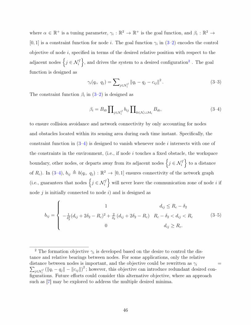
where α ∈ R+ is a tuning parameter, γi : R2 → R+ is the goal function, and βi : R2 →

[0, 1] is a constraint function for node i. The goal function γi in (3–2) encodes the control

objective of node i, specified in terms of the desired relative position with respect to the

adjacent nodesj ∈ N f

i

, and drives the system to a desired configuration2 . The goal

function is designed as

γi(qi, qj) =∑

j∈N fi‖qi − qj − cij‖2 . (3–3)

The constraint function βi in (3–2) is designed as

βi = Bi0

∏j∈N fi

bij∏

k∈Ni∪Mi

Bik, (3–4)

to ensure collision avoidance and network connectivity by only accounting for nodes

and obstacles located within its sensing area during each time instant. Specifically, the

constraint function in (3–4) is designed to vanish whenever node i intersects with one of

the constraints in the environment, (i.e., if node i touches a fixed obstacle, the workspace

boundary, other nodes, or departs away from its adjacent nodesj ∈ N f

i

to a distance

of Rc). In (3–4), bij , b(qi, qj) : R2 → [0, 1] ensures connectivity of the network graph

(i.e., guarantees that nodesj ∈ N f

i

will never leave the communication zone of node i if

node j is initially connected to node i) and is designed as

bij =

1 dij ≤ Rc − δ2

− 1δ22

(dij + 2δ2 −Rc)2 + 2

δ2(dij + 2δ2 −Rc) Rc − δ2 < dij < Rc

0 dij ≥ Rc.

(3–5)

2 The formation objective γi is developed based on the desire to control the dis-tance and relative bearings between nodes. For some applications, only the relativedistance between nodes is important, and the objective could be rewritten as γi =∑

j∈N fi(‖qi − qj‖ − ‖cij‖)2 ; however, this objective can introduce redundant desired con-

figurations. Future efforts could consider this alternative objective, where an approachsuch as [7] may be explored to address the multiple desired minima.

46

Also in (3–4), Bik , B(qi, qk) : R2 → [0, 1], for point k ∈ Ni ∪Mi, whereMi indicates the

set of obstacles within the sensing area of node i at each time instant, ensures that node i

is repulsed from other nodes or obstacles to prevent a collision, and is designed as

Bik =

−1δ21d2ik + 2

δ1dik dik < δ1

1 dik ≥ δ1.(3–6)

Similarly, the function Bi0 in (3–4) is used to model the potential collision of node i with

the workspace boundary, where the positive scalar Bi0 ∈ R is designed similar to Bik

by replacing dik with di0, where di0 ∈ R+ is the relative distance of the node i to the

workspace boundary defined as di0 = R− ‖qi‖.

Assumption 3.2 guarantees that γi and βi will not be zero simultaneously. The

navigation function candidate achieves its minimum of 0 when γi = 0 and achieves its

maximum of 1 when βi = 0. For ϕi to be a navigation function, it has to satisfy the

following conditions [29]:

1) smooth on F (at least a C1 function [38]);

2) admissible on F , (uniformly maximal on ∂F and constraint boundary);

3) polar on F , (qdi is a unique minimum);

4) a Morse function, (critical points3 of the navigation function are non-

degenerate).

If ϕi is a Morse function and qdi is a unique minimum of ϕi (i.e., qdi is polar on F), then

almost all initial positions (except for a set of points of measure zero) asymptotically

approach the desired position qdi [29]. In addition, the negative gradient of the navigation

function is bounded if it is an admissible Morse function with a single minimum at the

desired destination [29]. An example of the generated artificial potential field is shown in

3 A point p in the workspace F is a critical point if ∇qiϕi|p = 0.

47

−5

0

5 −5

0

5

0

0.5

1

0

0.1

0.2

0.3

0.4

0.5

0.6

0.7

0.8

0.9

1

Destination(minimum)

Obstacle(maximum)

Figure 3-1. An example of the artificial potential field generated for a disk-shapedworkspace with destination at the origin and an obstacle located at [1, 1]T .

Fig. 3-1, in which the destination is assigned a minimum potential value and the obstacle

is assigned a maximum potential value.

Based on the definition of the navigation function candidate, the decentralized

controller for each node is designed as

ui = −K∇qiϕi, (3–7)

where K is a positive gain, and ∇qiϕi is the gradient of ϕi with respect to qi. Hence, the

controller in (3–7) is bounded and yields the desired performance by steering node i along

the direction of the negative gradient of ϕi if (3–2) is a navigation function.

3.3 Connectivity and Convergence Analysis

The free configuration workspace Fi ⊂ F is a compact connected analytic manifold

for node i, Fi , q| βi(q) > 0, and q denotes the stacked position vector of node i. The

boundary of Fi is defined as ∂Fi, β−1

i (0). The narrow set around a potential collision for

node i is defined as

BBi,k(ε) , q| 0 < Bik < ε, ε > 0, k ∈ Ni ∪Mi,

48

and a narrow set around a potential connectivity constraint is defined as

Bbi,j(ε) , q| 0 < bij < ε, ε > 0, j ∈ N fi .

The set B0(ε) = q| 0 < Bi0 < ε, ε > 0 is used to denote a narrow set around a potential

collision of node i with workspace boundary. Inspired by the seminal work in [29], Fi is

partitioned into five subsets F0(ε), F1(ε), F2(ε), F3(ε), and Fdi(ε) as

Fi = Fdi ∪ F0(ε) ∪ F1(ε) ∪ F2(ε) ∪ F3(ε),

where the set of desired configurations for node i is defined as Fdi , q| γi(q) = 0. The

sets F0(ε), F1(ε), F2(ε) and F3(ε) describe the regions near the workspace boundary,

near the potential collision constraint, near the connectivity constraint and away from all

constraints for node i, respectively, and are defined as

F0(ε) , B0(ε)−Fdi,

F1(ε) ,⋃

ξi+ϑik=1 B

Bi,k(ε)−Fdi,

F2(ε) ,⋃ζi

j=1Bbi,j(ε)−Fdi,

and

F3(ε) , Fi − Fdi ∪ F0 (ε) ∪ F1 (ε) ∪ F2(ε) ,

where ξi, ϑi, ζi ∈ R+ denote the number of nodes in the set Ni,Mi and N fi , respectively.

Based on the partition of Fi, Proposition 3.1 to 3.8 are subsequently introduced to

ensure that the designed function in (3–2) is a navigation function. Proposition 3.1 shows

that network connectivity is ensured if the initial graph is connected. To establish the

convergence properties of the potential field, Proposition 3.2 shows the system converges

to the set of critical points under the controller in (3–7), and Proposition 3.3 to 3.8

49

together ensure that qdi is the unique minimum, and the other critical points are saddle

points, by proving that (3–2) has the properties of a navigation function. Proposition 3.3

shows qdi is a minimum in ϕi. Proposition 3.4 shows there is no minima on the workspace

boundary. Proposition 3.5 ensures all the critical points can be pushed away from F3(ε)

by choosing α big enough. Proposition 3.6 shows that ϕi is a Morse function, while

Proposition 3.7 and 3.8 indicate that the critical points in F0(ε), F1(ε) and F2(ε) are not

minima. Proposition 3.5 to 3.8 together guarantee that qdi is the unique minimum in the

workspace. The following assumptions are used to prove Proposition 3.6 to 3.8.

Assumption 3.3. No obstacles or other agents are assumed to stay within the collision

region of node i, when node i is very close to breaking the communication link with a node

j ∈ N fi (i.e., node i and node j belong to the region Bbi,j(ε)).

Assumption 3.4. The region BBi,k(ε) for k ∈ Ni ∪ Mi is disjoint. This assumption

implies a negligible probability of more than one simultaneous collision with node i.

3.3.1 Connectivity Analysis

Proposition 3.1. If the graph G is connected initially and j ∈ N fi , then (3–7) ensures

nodes i and j will remain connected for all time.

Proof. Proof: Consider node i located at a point q0 ∈ F that causes∏

j∈N fibij = 0, which

will be true when either only one node j is about to disconnect from node i or when more

than one node is about to disconnect with node i simultaneously. These two possibilities

are considered in the following two cases.

Case 1: There is only one node j ∈ N fi for which bij(q0, qj) = 0 and bil(q0, ql) 6= 0

∀l ∈ N fi , l 6= j. The gradient of ϕi with respect to qi is

∇qiϕi =αβi∇qiγi − γi∇qiβi

α(γαi + βi)1α

+1. (3–8)

Since bij = 0, the constraint function βi = 0 from (3–4). Thus, the gradient ∇qiϕi

evaluated at q0 can be expressed as ∇qiϕi|q0 = −γi∇qiβiαγα+1

i

∣∣∣q0. Based on the fact that βi can

50

be expressed as the product βi = bij bij, where

bij(q0, qj) = Bi0

∏l∈N fi ,l 6=j

bil∏

k∈Ni∪Mi

Bik, (3–9)

and ∇qibij is computed as

∇qibij =

0 dij < Rc − δ2 or dij > Rc

−2(dij+δ2−Rc)(qi−qj)δ22dij

Rc − δ2 ≤ dij ≤ Rc,(3–10)

the gradient of βi evaluated at q0 can be obtained as ∇qiβi|q0 = −2bijδRc

(qi − qj). Since Ki, γi,

α, bij and δ are all positive terms, (3–7), and ∇qiβi|q0 can be used to determine that the

controller (i.e., the negative gradient of ∇qiϕi) is along the direction of qj − qi, which

implies node i is forced to move toward node j to ensure connectivity. That is, based on

the design of bij in (3–5) and its gradient in (3–10), whenever a node enters the escape

region of node i, an attractive force is imposed on node i to ensure connectivity.

Case 24 : Consider two nodes j, l ∈ N fi , where bij = 0 and bil = 0 (i.e., ‖qi − qj‖ = Rc

and ‖qi − ql‖ = Rc) simultaneously. In this case, βi = 0 and ∇qiβi is a zero vector, (3–8)

can be used to determine that q0 is a critical point (i.e., ∇qiϕi|q0 = 0), and the navigation

function achieves its maximum value at the critical point (i.e., ϕi|q0 = 1). Since ϕi is

maximized at q0, no open set of initial conditions can be attracted to q0 under the control

law designed in (3–7).

From the development in Case 1 and Case 2, the control law in (3–7) ensures that all

nodes j ∈ N fi remain connected with node i for all time.

4 Case 2 can be extended to more than two nodes without loss of generality.

51

3.3.2 Convergence Analysis

Proposition 3.2. The system in (3–1) converges to the largest invariant set (i.e., the set

of critical points S =q| ∇qiϕi|q = 0

) under the controller in (3–7), provided that the

tuning parameter in (3–2) satisfies α > Θ, where Θ = max

√|c1|c3, |c2|

c3

.

Proof. Consider a Lyapunov candidate V (q) =∑N

i=1 ϕi, where q is the stacked states of

all nodes, i.e., q = [q1, · · · , qN ]T . The time derivative of V is computed as

V = (∇V )T q = −K∑N

i=1

∑N

j=1(∇qiϕi)

T (∇qiϕj) ,

which can be further separated as

V = −K∑

i:∇qiϕi=0

(‖∇qiϕi‖

2 +∑

j 6=i(∇qiϕi)

T (∇qiϕj))

−K∑

i:∇qiϕi 6=0

(‖∇qiϕi‖

2 +∑

j 6=i(∇qiϕi)

T (∇qiϕj)). (3–11)

When all nodes are located at the critical points in (3–11), V = 0. To show that the set of

critical points are the largest invariant set, it requires that V is strictly negative, whenever

there exists at least one node i such that ∇qiϕi 6= 0. Since ∇qiϕi 6= 0 for at least one node,

(3–11) can be rewritten as

V = −K∑

i:∇qiϕi 6=0

(‖∇qiϕi‖

2 +∑

j 6=i(∇qiϕi)

T (∇qiϕj)). (3–12)

To ensure that V < 0 in (3–12), it is sufficient to require that∑

j 6=i (∇qiϕi)T (∇qiϕj) > 0,

which can be expanded by using (3–8) as(βi∇qiγi −

γiα∇qiβi

)T(γαi + βi)

1α

+1

(∑j 6=i

(βj∇qiγj −

γjα∇qiβj

)(γαj + βj)

1α

+1

)> 0. (3–13)

Since γi, βi are all positive from (3–3) and (3–4), and γi, βi can not be zero simultaneously

from Assumption 3.2, the inequality in (3–13) is valid provided

(βi∇qiγi −

γiα∇qiβi

)T (∑j 6=i

(βj∇qiγj −

γjα∇qiβj

))> 0,

52

which can be simplified as1

α2c1 +

1

αc2 + c3 > 0, (3–14)

where

c1 = γi (∇qiβi)T∑

j 6=iγj∇qiβj,

c2 = −βi (∇qiγi)T∑

j 6=iγj∇qiβj − γi (∇qiβi)

T∑

j 6=iβj∇qiγj,

and

c3 = βi (∇qiγi)T∑

j 6=iβj∇qiγj.

In (3–14), since βi and βj are positive, and node i satisfies ∇qiϕi 6= 0, c3 is positive from

(3–3). Using the fact that c1 ≥ − |c1| , c2 ≥ − |c2|, (3–14) can be written as

− 1

α2|c1| −

1

α|c2| > −c3,

which suffices to show that α > max

√|c1|c3

and α > max

|c2|c3

. Therefore, if α is

chosen such that α > Θ, where Θ = max

√|c1|c3, |c2|

c3

, the system converges to the set of

critical points.

Proposition 3.3. The navigation function is minimized at the desired point qdi.

Proof. The navigation function ϕi is minimized at a critical point if the Hessian of ϕi

evaluated at that point is positive definite. The gradient expression in (3–8) is used to

determine if qdi is a critical point. From the definition of qdi and (3–3), the goal function

evaluated at the desired point is γi|qdi = 0. Also, the gradient of the goal function

evaluated at the desired point qdi is

∇qiγi|qdi =∑j∈N fi

2(qdi − qj − cij) = 0.

53

Since γi|qdi = 0 and ∇qiγi|qdi = 0, (3–8) can be used to conclude that ∇qiϕi|qdi = 0. Thus,

the desired point qdi in the workspace F is a critical point of ϕi. The Hessian of ϕi is

∇2qiϕi =

1

α(γαi + βi)1α

+2

(γαi + βi)

[α∇qiβi (∇qiγi)

T −∇qiγi(∇qiβi)T + αβi∇2

qiγi

−γi∇2qiβi]− α + 1

α[αβi∇qiγi − γi∇qiβi] ·

[αγα−1

i ∇qiγi +∇qiβi]T

. (3–15)

Using the facts that γi|qdi = 0 and ∇qiγi|qdi = 0 and the Hessian of γi is

∇2qiγi = 2ζiI2, (3–16)

where I2 is the identity matrix in R2×2, the Hessian of ϕi evaluated at qdi is given by

∇2qiϕi∣∣qdi

= 2β− 1α

i I2ζi.

The constraint function βi > 0 at the desired configuration by Assumption 3.2, and ζi is a

positive number. Hence, the Hessian of ϕi evaluated at that point is positive definite.

Proposition 3.4. No minima of ϕi are on the boundary of the free workspace Fi.

Proof. Consider a point q0 ∈ ∂Fi . From the definition of ∂Fi the constraint function

βi(q0) = 0. The goal function γi is zero only at the desired configuration point, and from

Assumption 3.2, the desired configuration cannot be on the boundary of Fi. Thus, the

goal function γi evaluated at q0 is not zero. Using (3–2) and the facts that βi|q0 = 0 and

γi|q0 6= 0, ϕi|q0 is maximized at any arbitrarily chosen point q0 on the boundary of Fi.

Proposition 3.5. For every ε > 0, there exists a number Γ(ε) such that if α > Γ(ε) no

critical points of ϕi are in F3(ε).

Proof. From (3–8), any critical point must satisfy αβi∇qiγi = γi∇qiβi. If α is chosen as

α > supγi ‖∇qiβi‖βi ‖∇qiγi‖

,

54

where sup is taken over F3(ε), then from (3–8), ϕi will have no critical points in F3(ε).

Since ε = inf bij = inf Bik in F3(ε), an upper bound supγi‖∇qiβi‖βi‖∇qiγi‖

is given as

supγi

‖∇qiγi‖‖∇qiβi‖βi

≤ Γ(ε)

where

Γ(ε) , supγi

‖∇qiγi‖

(∑ζi

j=1,j 6=i

sup ‖∇qibij‖ε

+∑ξi+ϑi

k=0,k 6=i

sup ‖∇qiBik‖ε

). (3–17)

In (3–17), ‖∇qibij‖, ‖∇qiBik‖ and γi

‖∇qiγi‖are bounded terms in F3(ε) from (3–3), (3–10)

and the fact that

∇qiBik =

(− 2δ21dik + 2

δ1) qi−qkdik

dik < δ1

0 dik ≥ δ1.(3–18)

Proposition 3.6. There exists ε0 > 0 such that if ε < ε0, then ϕi is a Morse function.

Proof. The development in [30] and [39] proves that for ϕi to be a Morse function, it is

sufficient to show that uT (∇2qiϕi∣∣qci

)u is positive for some particular vector u by choosing

a small ε, where qci is a critical point. To show that uT (∇2qiϕi∣∣qci

)u is positive for the unit

vector

u ,qi − qj‖qi − qj‖

,

(3–15) is used and the Hessian ∇2qiϕi evaluated at qci is

αuT(∇2qiϕi∣∣qci

)u

(γαi + βi)− 1α−1

= uT

(αβi∇2

qiγi +

(1− 1

α

)γi

βi∇qiβi (∇qiβi)

T − γi∇2qiβi

)u (3–19)

To facilitate the subsequent analysis, the set of critical points in Fi is divided into sets

of critical points in regions F0(ε), F1(ε), and F2(ε). For a case where a critical point

55

qci ∈ F2(ε), using the fact that ∇qiβi and ∇2qiβi can be expressed as

∇qiβi = bij∇qibij + bij∇qi bij, (3–20)

∇2qiβi = bij∇2

qibij +

(∇qi bij∇T

qibij +∇qibij∇T

qibij)

+ bij∇2qibij, (3–21)

where bij is defined in (3–9), and the fact that the first term on the right hand side of

(3–19) is always positive from (3–16), the subsequent expression can be obtained as

α(γαi + βi)1α

+1uT(∇2qiϕi∣∣qci

)u > γiΩ, (3–22)

where

Ω =1

bij

(a1b

2ij + a2bij + a3

),

with

a1 =(α− 1)

∥∥∇qi bij∥∥2

αbij− uT (∇2

qibij)u,

a2 =2(α− 1)(∇qi bij)

T (∇qibij)

α− bijuT (∇2

qibij)u− uT

(∇qi bij∇T

qibij +∇qibij∇T

qibij)u,

and

a3 =(α− 1)bij

α‖∇qibij‖

2 .

Since bij > 0, a necessary condition to show that Ω > 0 is to prove that

a1b2ij + a2bij + a3 > 0, (3–23)

where a3 > 0 if α > 1. To prove the inequality in (3–23), the following two cases are

analyzed.

Case 1: For a1 < 0, the inequality in (3–23) is valid if

bij <−a2 −

√a2

2 − 4a1a3

2a1

.

56

Case 2: For a1 ≥ 0, Ω can be rewritten as Ω ≥ a2 + a3bij, which is positive if

bij <a3

|a2|.

Therefore, Ω > 0, and from (3–22), uT (∇2qiϕi∣∣qci

)u > 0 for all cases if bij is chosen as

bij < ε′

0 , min

−a2 −

√a2

2 − 4a1a3

2a1

,a3

|a2|

.

By using the same process of evaluating the Hessian ∇2qiϕi at critical points belonging

to F0(ε) and F1(ε), upper bounds ε′′0 and ε′′′0 for ε can be obtained for qci ∈ F1(ε) and

qci ∈ F0(ε) respectively. By choosing ε < ε0 = minε′0, ε

′′0 , ε

′′′0

, the function Ω is

guaranteed to be positive which implies all the critical points are non-degenerate critical

points of ϕi.

Proposition 3.7. There exists ε1 > 0, such that ϕi has no local minimum in F2(ε), as

long as ε < ε1.

Proof. Consider a critical point qci ∈ F2(ε). Since ϕi is a Morse function, then if ∇2qiϕi∣∣qci

has at least one negative eigenvalue, ϕi will have no minimum in F2(ε). To show ∇2qiϕi∣∣qci

has at least one negative eigenvalue, a unit vector

v ,

(∇qiβi‖∇qiβi‖

)⊥is defined as a test direction to demonstrate that

vT(∇2qiϕi∣∣qci

)v < 0,

where (χ)⊥ denotes a vector that is perpendicular to some vector χ. Using (3–20) and

(3–21),

α(γαi + βi)1α

+1∣∣∣qcivT(∇2qiϕi∣∣qci

)v = −γiΦ + bijΨ,

where

Φ = vT(∇qi bij∇T

qibij +∇qibij∇T

qibij − bij∇2

qibij)v,

57

Ψ = vT(αbij∇2

qiγi − γi∇2

qibij)v,

and

∇2qibij =

0 dij ≤ Rc − δ2 or dij ≥ Rc

2(δ2−Rc)(qi−qj)(qi−qj)Tδ22d

3ij

− 2(dij+δ2−Rc)dijδ22

I2 Rc − δ2 < dij < Rc.(3–24)

Based on Assumption 3.3 and (3–5), (3–6), (3–10), (3–24), ∇qi bij = 0 and ∇2qibij < 0. Since

the goal function γi and bij are positive, Φ > 0. To ensure vT(∇2qiϕi∣∣qci

)v < 0, ε must be

selected as ε < ε1 where ε1 = infF2(ε)|γiΦ||Ψ| .

Proposition 3.8. There exists ε2 > 0, such that ϕi has no local minimum in F1(ε) and

F0(ε), as long as ε < ε2.

Proof. Consider a critical point qci ∈ F1(ε). Similar to the proof for Proposition 3.7, the

current proof is based on the fact that if wT(∇2qiϕi∣∣qci

)w < 0 for some particular vector

w ,(

qi−qk‖qi−qk‖

)⊥, then ϕi will have no minimum in F1(ε). To facilitate the subsequent

analysis, similar to the definition of bij in (3–9), βi can be expressed as the product

βi = BikBik and Bik is defined as

Bik(qi, qk) = Bi0

∏j∈N fi

bij∏

l∈Ni∪Mi,l 6=kBil. (3–25)

Using (3–16), (3–18) and (3–25),

α(γαi + βi)1α

+1∣∣∣qciwT(∇2qiϕi∣∣qci

)w = γiBikΛ + γiBikΞ,

where

Λ = ∇TqiBik

∇qiγi‖∇qiγi‖

2ζi −2(δ1 − dik)dikδ2

1

,

Ξ = wT

(∇TqiBik∇qiγi

‖∇qiγi‖∇2qiγi +

(1− 1α

)

βij∇qiBik∇T

qiBik −∇2

qiBik

)w,

and

∇2qiBik =

(− 2δ21

+ 2dikδ1

)I2 − 2(qi−qk)(qi−qk)T

δ1d3ikdik < δ1

0 dik ≥ δ1..

58

Since dik < δ1, and ∇TqiBik

∇qiγi‖∇qiγi‖

can be upper bounded by a positive constant in F1(ε),

then if dik is small enough, Λ is guaranteed to be negative. Hence, there exist a positive

scalar ε21 = Bik(dik), which is small enough to ensure Λ < 0. To ensure

wT(∇2qiϕi∣∣qci

)w < 0,

ε must be selected as

ε < minε21, infF1(ε)

∣∣ΛBik

∣∣|Ξ|

.

Let x be an unit vector defined as

x ,

(qi − q0

‖qi − q0‖

)⊥.

The same procedure that was used to show

wT(∇2qiϕi∣∣qci

)w < 0

in F1(ε) can be followed to obtain another upper bound for ε, which ensures

xT(∇2qiϕi∣∣qci

)x < 0

in F0(ε). By choosing ε2 as the minimum of the upper bound for ε developed for F1(ε)

and F0(ε), ϕi is ensured to have no minimum in F1(ε) and F0(ε) as long as ε < ε2.

Based on Propositions 3.2 to 3.8, if ε is chosen such that ε ≤ min ε0, ε1, ε2 then the

minima (a critical point) is not in F0(ε), F1(ε), F2(ε), F3(ε) or the boundary of Fi. Thus,

the minima has to be in Fdi(ε) if α > max1,Γ(ε),Θ. Hence, nodes starting from any

initial positions (except for the unstable equilibria) will converge to the desired formation

specified by the formation matrix cij.

3.4 Simulation

Simulation results illustrate the performance of the proposed control strategy. As

shown in the Fig. 3-2, a connected initial graph of 40 nodes with kinematics in (3–1) are

deployed with desired neighborhood in a workspace of R = 30 m with static obstacles.

59

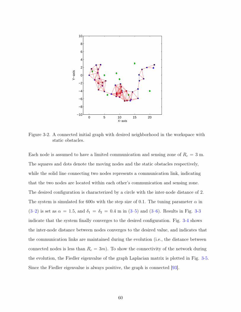
0 5 10 15 20−10

−8

−6

−4

−2

0

2

4

6

8

10

X−axis

Y−

axis

Figure 3-2. A connected initial graph with desired neighborhood in the workspace withstatic obstacles.

Each node is assumed to have a limited communication and sensing zone of Rc = 3 m.

The squares and dots denote the moving nodes and the static obstacles respectively,

while the solid line connecting two nodes represents a communication link, indicating

that the two nodes are located within each other’s communication and sensing zone.

The desired configuration is characterized by a circle with the inter-node distance of 2.

The system is simulated for 600s with the step size of 0.1. The tuning parameter α in

(3–2) is set as α = 1.5, and δ1 = δ2 = 0.4 m in (3–5) and (3–6). Results in Fig. 3-3

indicate that the system finally converges to the desired configuration. Fig. 3-4 shows

the inter-node distance between nodes converges to the desired value, and indicates that

the communication links are maintained during the evolution (i.e., the distance between

connected nodes is less than Rc = 3m). To show the connectivity of the network during

the evolution, the Fiedler eigenvalue of the graph Laplacian matrix is plotted in Fig. 3-5.

Since the Fiedler eigenvalue is always positive, the graph is connected [93].

60

0 5 10 15 20 25

−5

0

5

10

15

20

X−axis

Y−

axis

Figure 3-3. The achieved final configuration.

0 100 200 300 400 500 6000

0.5

1

1.5

2

2.5

3

time

Inte

r−no

de d

ista

nce

Figure 3-4. The inter-node distance during the evolution

61

0 100 200 300 400 500 6000.015

0.02

0.025

0.03

0.035

0.04

0.045

0.05

0.055

0.06

0.065

time

Fie

dler

eig

enva

lue

Figure 3-5. The plot of the Fiedler eigenvalue of the Laplacian matrix during theevolution. The circle indicates the Fiedler eigenvalue of the graph at each timeinstance.

3.5 Summary

Given an initial graph with a desired neighborhood, a navigation function based

decentralized controller is developed to ensure the system asymptotically converges to the

desired configuration while maintaining network connectivity and avoiding collisions with

other agents and obstacles. A distinguishing feature of the developed approach is that

the distributed agents achieve a coordinated global configuration without requiring radio

communication. Future efforts are focused on enabling radio-silent navigation from an

arbitrarily connected distributed network. Moreover, further efforts are required to elim-

inate Assumption 3.3 so that other obstacles or agents can be within the collision region

of node i when node i is about to break the communication link. Likewise Assumption 3.4

becomes less practical as a point grows to a sphere in the presence of uncertainty, and as

the workspace becomes more crowded. Future work is required to address the pervasive

problem of obstacle avoidance in a cluttered workspace with uncertainty.

62

CHAPTER 4NETWORK CONNECTIVITY PRESERVING FORMATION RECONFIGURATION

FOR IDENTICAL AGENTS FROM AN ARBITRARY CONNECTED INITIAL GRAPH

A navigation function based decentralized method is developed in Chapter 3 to

stabilize a group of agents in a desired formation while maintaining network connectivity.

However, an assumption in Chapter 3 is that the initial topology is required to be

a supergraph of the desired topology ensuring the agents are originally in a feasible

interconnected state. Such initial graph assumption may limit its applications which

require agents to achieve desired formations from an arbitrary initial graph or dynamically

change the achieved formations to adapt to an uncertain environment. The focus of this

chapter is to control a group of identical agents to achieve a desired formation from an

arbitrarily connected initial condition, while preserving network connectivity during the

motion. A novel network topology labeling algorithm developed in the work [52] is applied

in this chapter to dynamically specify the neighborhood of each agent in the initial graph

according to the desired formation, and determine the required movement for all nodes

to achieve the desired formation. One distinguishing feature of this approach is that we

do not wish to specify which nodes in the initial topology will take which positions in

the final topology; rather, we only care that there is an agent in each position specified

in the final topology. By modeling the network connectivity as an artificial obstacle, a

navigation function based control scheme developed in our previous work of [94] is applied

to guarantee the network connectivity by maintaining the neighborhood among agents

determined by the prefix labeling algorithm, and ensure the convergence of all agents to

the desired configuration with collision avoidance among agents using local information

(i.e., local sensing and communication). An information flow is also proposed to specify

the required movement for extra agents to their destination nodes. The information

flow-based approach generally provides a path with more freedom for the motion of extra

nodes without partitioning the network connectivity and allows communication links

63

to be formed or broken in a smooth manner without introducing discontinuity. Finally,

convergence is proven using Rantzer’s Dual Lyapunov Theorem [55].

4.1 Problem Formulation

Consider a network composed of N agents in workspace F , where agent i moves

according to

qi = ui, i = 1, · · · , N (4–1)

where qi = [xi yi]T ∈ R2 denotes the position of agent i in a two dimensional (2D) plane,

and ui ∈ R2 denotes the velocity of agent i (i.e., the control input). The workspace F is

assumed to be circular and bounded with radius R. Each agent in F is assumed to be a

point-mass with limited communication and sensing capability encoded by a local disk

area. For simplicity and without loss of generality, the following development is based on

the assumption that the sensing zone is the same as the communication zone, both with

radius Rc. Two moving agents can communicate with each other if the relative distance is

less than the radius Rc. All the agents are assumed to be identical with equal actuation

capabilities. Each agent is assumed to have real-time knowledge of its own states.

Since each agent can only sense and communicate with other agents located

within the distance Rc, the interaction among agents is modeled as an undirected

graph G = (V , E (t)), with V denoting the index set of all nodes and the set of edges

E = (i, j) ∈ V × V| dij ≤ Rc , where node i and j represent agents located at posi-

tion qi and qj, and dij ∈ R+ is the distance between them, defined as dij = ‖qi − qj‖ .

The edge (i, j) denotes a bidirectional communication link between node i and j, indi-

cating that node i and j have access to the states of each other. The neighborhood of

node i, Ni, (i.e., all the agents within the communication zone of agent i), is given by

Ni = j, j 6= i| j ∈ V , (i, j) ∈ E , which is a time-varying set, since other nodes may enter

or leave the communication region of node i at any time. The desired configuration is

characterized by the specified relative position between nodes i and j ∈ N fi , where N

fi

denotes the set of neighbors for node i in Gf , and the desired position qdi for node i is

64

Figure 4-1. The small disk area with radius δ1 denotes the collision region and the outerring area denotes the escape regions for node i. The region in the sensing zoneapart from collision and escape regions denotes the free-motion region.

defined as

qdi =qi| ‖qi − qj − cij‖2 = 0, j ∈ N f

i

, (4–2)

where cij ∈ R2 represents the desired relative position between node i and j.

A collision region is defined for each agent i as a small disk area with radius δ1 < Rc

around the agent i, such that any other agent j ∈ V inside this region is considered as a

potential collision with agent i. To ensure connectivity, an escape region for each agent i

is defined as the outer ring of the communication area with radius r, Rc − δ2 < r < Rc,

where δ2 ∈ R is a predetermined buffer distance. Edges formed with a node j ∈ Ni in

the escape region are in danger of breaking. Agent i moves with the constraint of avoiding

a collision with other agents located in the collision region, and preventing a break in

the communication link between agents located in the escape region. The collision and

escape regions for agent i are shown in Fig. 4-1. The region within the sensing zone can

be considered as the free-motion region where an agent can move freely.

Let Gi denote the initial network topology and Gf denote the desired final topology.

The subsequent development is based on the following assumptions.

65

Assumption 4.1. The initial graph associated with Gi is connected and the initial

positions do not coincide with some unstable equilibria (i.e., saddle points).

Assumption 4.2. Gf is a tree, and all nodes in Gi are assumed to have a knowledge of Gf

before applying the network topology labeling algorithms. The desired formation associated

with Gf is specified in advance and valid, which implies that the desired configuration is

connected and will not lead to a collision or the desired configuration will not lead to a

partitioned graph, i.e., δ1 < ‖cij‖ < Rc − δ2.

4.2 Formation Reorganization Strategy

To achieve a desired formation from an arbitrary initial graph while preserving

network connectivity, the developed formation reorganization strategy has two stages:

a networking-based labeling and routing algorithm over the network topology, and a

potential field based motion control algorithm on the physical graph. Given an arbitrary

initial graph, a labeling and routing algorithm is used to assign each agent a unique

label, specify which node in the initial topology should take which position in the final

topology, and determine how the initial topology can be transformed into the desired

topology, all while preserving the network connectivity. After the network topology has

been determined, a motion control algorithm is implemented to physically steer each

agent toward a desired location based on the physical topology while maintaining network

connectivity.

Specifically, the prefix labeling and routing algorithm subsequently described in

Section 4.3 is first applied on the initial network graph to form a prefix tree by labeling

the identical agents. A prefix tree is commonly called a trie [95]. A key observation is

that, for arbitrary initial and desired final topologies, there are always spanning trees that

eliminate loops while preserving connectivity. Before assigning prefix labels, the initial

network topology may not be a tree. However, after assigning prefix labels, the network

can be formed as a trie, and the length of the label corresponds to its depth in the trie.

Once the trie is established, the initial trie topology can be reconfigured to a desired trie

66

topology by moving some agents. The novel idea is that the agents can be treated as

packets that are then routed through the network. Hence, the agents can be moved toward

its destination as routing a packet through the network. A distinguishing advantage

of using prefix labeling and routing is that topology reconfiguration can be achieved

from an arbitrary initial topology, since the labels, destinations and neighborhood for

agents are dynamically determined, instead of being specified in advance like results such

as [9, 39, 41, 45–48]. However, the prefix labeling and routing approach in Section 4.3

requires global communication for each agent to determine its own label and broadcast

its label to other agents through the overall network. Since the agents are not physically

moved in this stage, the prefix labeling procedure can be done in an off-line fashion for

the given initial graph. Once the first stage is complete, the potential field based motion

control algorithm developed in Section 4.4 is then applied to steer the agents to the

desired formation while preserving network connectivity. Note that only local sensing and

communication is used for the formation stabilization in the second stage.

4.3 Network Topology Labeling Algorithms

A prefix labeling and routing algorithm is developed in this section to label the

agents with prefix, specify the neighborhood for each node in Gi. Since some nodes (i.e.,

extra nodes) are required to be repositioned to achieve Gf , the proposed algorithm also

determines the destination and path for each extra node to achieve Gf while preserving

network connectivity.

4.3.1 Basic Algorithm

A trie Gt is generated from Gi by randomly selecting a node in Gi to be the root

and letting the selected root assign a prefix label to each node in Gi in breadth-first

fashion [96]. For instance, in a simple form of prefix labeling, one node is elected to be the

root. The neighbors of the root are labeled as children of the root in a prefix tree. Then

those nodes label their children, and the process continues until each node has a unique

67

label1 . The prefix label assigned to each node serves as its network address. To illustrate

the prefix labeling algorithm, an example is provided Fig. 4-2, where the root is assigned

the label 0. The children of the root are then assigned the labels 01, 02, 03 and 01, 02

in Fig. 4-2 (a) and Fig. 4-2 (b) respectively.

By identifying nodes in Gt that do not match the desired topology Gf , the node that

is missing children is denoted as a requesting node, and the node whose label does not

exist in Gf is called an extra node. Each requesting node sends the root a message, M.Req,

that includes a list of its missing children addresses. A copy of this message will also be

stored at all nodes who are located along the path to the root. At the same time, each

extra node also sends a message, M.Label, including its own label to the root. Once the

root obtains all the messages from these nodes, the root will ask each extra node to move

one-by-one starting from an extra node with the longest label (i.e., the extra node that is

deepest in the trie). The extra node with the longest prefix label is moved first to preserve

the network connectivity during the process. If an extra node is a parent of other extra

nodes, the other extra node will be orphaned and thus may loose network connectivity if

the parent node moves first.

In prefix routing, the extra node first finds out the destination node’s prefix label,

and then uses maximum prefix matching logic [49–51] to route themselves to the desired

destination through the network. This extra node will check for cached M.Req messages

in the nodes which are located along the way to the root for the missing node address. If

there exists more than one missing node address, the extra node will decide to move to

the closest missing node by comparing the prefix label of the missing node address and

the current node address. Whenever this extra node reaches its parent requesting node

1 Because of the loops in the graph, the labeling is not unique. That is, for a givengraph, there may exist several different sets of labeling. However, in each individual set oflabeling, each agent has a unique prefix label.

68

in Gf , the requesting node will send a message, M.RCM, to the root confirming that it

has received an extra node, and the extra node will be relabeled to take the role of the

formerly missing node in the desired topology. This message also tells all the nodes along

the path to the root to delete this missing node address from their cache. When the root

obtains M.RCM, it will initiate the process again by asking the extra nodes at the next

level in the trie to move. This process will continue until the desired network topology is

achieved.

Fig. 4-2 is provided to illustrate the prefix routing algorithm. The node 03 and 031

in Fig. 4-2 (a) are extra nodes, since they do not exist in the Fig. 4-2 (b) by comparing

the prefix labels in the initial and the desired topology in Fig. 4-2. To achieve the desired

topology shown in Fig. 4-2 (b), node 031 is required to move first toward the node 01

through the path 031, 03, 0, 01, since node 031 has the longest label among all the extra

nodes. Once a new edge between node 01 and 031 is created, 031 is relabeled by 011, and

following a similar process, node 03 then starts to move toward node 01 to fill the rest

vacancy of 012 in Fig. 4-2 (b).

The time required to transition to the final topology can be reduced by allowing

some extra nodes to move simultaneously. In Destination Assignment Algorithm, the

root assigns each extra node a destination by sending them a message M.Dest, which

includes the requesting node address. Pseudocode for Destination Assignment Algorithm

is provided in Algorithm 4.1. In a tree topology, leaf nodes are those nodes who do not

have children. Thus, leaf nodes can be repositioned without affecting network connectivity.

If an extra node is a leaf node, it can move whenever it receives a message M.Dest, but

other nodes have to wait for their children to move up the tree before the parent can

move. An extra node that reaches the destination first will be immediately relabeled and

forwarded by the requesting node to fulfill the desired network trie. If more than one

extra node reach the destination requesting node at the same time, the requesting node

will check the hop number of each extra node by comparing the extra node label with

69

1 2 3 4 5 60.5

1

1.5

2

2.5

3

3.5

4

4.5

5

5.5

031

0

03

02

01

021

022

(a) Initial Network Topology

0 1 2 3 4 51

1.5

2

2.5

3

3.5

4

4.5

5

5.5

6

0

01 02

011 012 021 022

(b) Desired Network Topology

Figure 4-2. The example of an initially connected and desired graph topology, where thenodes denote the agent, and the lines connecting two nodes denote theavailable communication links. In Fig. 4-2 (a) and (b), the root is assigned thelabel 0. The children of the root are then assigned the labels 01, 02, 03 and01, 02 in Fig. 4-2 (a) and (b) respectively. Other nodes such as 021, 022,031 and 011, 012, 021, 022 are labeled by following a similar procedure.

its prefix. Then the requesting node will assign those nodes to its subtree to minimize

the number of hops each node must travel. That is, nodes that have already traveled the

largest number of hops will be assigned as children of the requesting node, whereas extra

nodes that have traveled few hops will be assigned as the leaf nodes of the deepest part of

the subtree.

4.3.2 Relabeling Algorithm

The performance of reorganizing the network topology is highly dependent on how

the prefix labels are assigned in Gi. To improve the performance of reorganization, Branch

Relabeling (BR) and Neighbor Relabeling (NR) methods are developed to relabel the

nodes in trie Gt. Before applying these algorithms, Gi is required to be prefix-labeled via

the Basic Algorithm in the previous subsection, to form a trie Gt. Pseudocode for Branch

Relabeling and Neighbor Relabeling are provided in Algorithm 4.2 and Algorithm 4.3.

70

Algorithm 4.1 Destination Assignment1: procedure Input:(extranodes)

. extra node labels2: groups = GroupByPrefixLength(extranodes);

. Starting from the longest lengths group3: for G ∈ groups 3 G.length == max (groups.length) do4: searchBackDepth = 1;5: for node ∈ G do6: node.DestinationAssigned = false;7: end for8: while ∃node ∈ G 3 node.DestinationAssigned == false do9: for node ∈ G 3 node.DestinationAssigned == false do

. Each time through this loop, search starting at ancestor that issearchBackDepth toward the root.

10: parent = node;11: for i = 1 to searchBackDepth do12: parent = GetNodeParent(parent);13: end for14: requestingNode = SearchSubtreeForClosestMissingNode(parent);15: if requestingNode 6= ∅ then16: node.DestinationAddress = requestingNode;17: node.DestinationAssigned = true;18: end if19: end for20: searchBackDepth++;21: end while22: groups = groups - G;23: end for24: end procedure

71

4.3.2.1 Branch Relabeling (BR) Algorithm

In the BR algorithm, the total amount of node movement required to achieve the

desired network topology can be reduced by swapping the nodes prefix labels in two or

more branches. Each leaf node sends a message including its label to the root. Once the

root has the knowledge of all the node prefix labels in the network, starting from the

root, nodes can then consider swapping the prefix label associated with two branches of

descendants. In this work, branch relabeling is only applied at the root, since the root is

most likely to have the largest impact on the amount of movement required to achieve

the desired topology. An example BR algorithm is illustrated in Fig. 4-3, where the

marked nodes denote the extra nodes, and the solid lines connecting two nodes indicate

the required edges in the desired topology, shown in Fig. 4-2 (b). Before applying the BR

algorithm, both node 03 and 031 are required to move all the way to node 01 to achieve

the desired topology. After applying the BR algorithm, less movement is required since

only node 03 is required to move.

Algorithm 4.2 Branch Relabeling Algorithm1: procedure Input:(Node)

. all node including label in the graph2: RootChild = GetRootChild(Node);3: RootChildSwap = AllSwap(RootNeighbor);

. obtain all swapping label pattern of all root neighbor4: for p ∈ RootChildSwap do5: Nodetemp = BRLabel(Node, p);

. Relabel all nodes in each branch according to p6: HopNum(p) = GetHopNum(Nodetemp);

. obtain the total hop number required for p7: end for8: p = MinHop(HopNum);

. obtain p achieving minimum total hop required9: Node = BRLabel(Node, p);

. Relabel each node according to p achieving minimum total hop required10: end procedure

72

1 2 3 4 5 60.5

1

1.5

2

2.5

3

3.5

4

4.5

5

5.5

031

0

03

02

01

021

022

(a) Before Performing BR Algorithm

1 2 3 4 5 60.5

1

1.5

2

2.5

3

3.5

4

4.5

5

5.5

011

0

01

02

03

021

022

(b) After Performing BR Algorithm

Figure 4-3. Fig (a) and (b) illustrates a graph before performing BR algorithm and afterperforming BR algorithm respectively, where the shaded nodes denote theextra nodes, the solid lines indicate the required edges in the desired topologyin Fig. 4-2(b), and the dashed line indicate the available communication linksbut not required to maintain for the desired topology.

4.3.2.2 Neighbor Relabeling (NR) Algorithm

The NR method is designed to relabel the extra nodes by exploiting additional

connections that exist in Gi to reduce the number of nodes required to move. All the

nodes first check if they are extra nodes and reset the labels of extra nodes as null. Once

the role of extra nodes is identified, all nodes that are missing children in Gf will check if

some of the extra nodes are their neighbors in Gi. If so, the node that is missing children

will relabel the neighboring extra node by sending it a message, M.Relabel. The process

is repeated until no more relabeling is possible. Then, all remaining extra nodes will be

labeled by their neighbors to form Gt. An example NR algorithm is illustrated in Fig.4-4.

Given an initial topology with prefix labeling as shown in Fig. 4-4 (a), two extra nodes are

identified. After applying the NR algorithm, only one extra node is identified in Fig.4-4

(b).

73

For dense networks (in which the number of edges is high), NR may offer advantages

over BR since NR can exploit the many network connections. In most cases, NR and BR

can be combined to offer the greatest benefit across initial network topologies.

Algorithm 4.3 Neighbor Relabeling Algorithm1: procedure Input:(Node)

. all node including label in the graph2: RootChild = GetRootChild(Node);3: RootChildSwap = AllSwap(RootNeighbor);

. obtain all swapping label pattern of all root neighbor4: for p ∈ RootChildSwap do5: Nodetemp = BRLabel(Node, p);

. Relabel all nodes in each branch according to p6: HopNum(p) = GetHopNum(Nodetemp);

. obtain the total hop number required for p7: end for8: p = MinHop(HopNum);

. obtain p achieving minimum total hop required9: Node = BRLabel(Node, p);

. Relabel each node according to p achieving minimum total hop required10: end procedure

4.4 Control Design

Section 4.3 describes how to determine the neighborhood for each node in Gi accord-

ing to the desired Gf . This section will discuss about how to physically move all nodes to

achieve the desired formation with topology Gf , while maintaining network connectivity.

Information flow is introduced to indicate the required communication for extra nodes. A

potential field based decentralized control strategy is then developed to guide the extra

nodes to their destinations, and ensure all nodes converge to the desired formation with

collision avoidance among nodes while maintaining network connectivity.

4.4.1 Information Flow

Assume that the Gi and Gf are already prefix labeled. To achieve the desired cij

in (4–2) for ∀i and j ∈ N fi , a neighborhood between node i and j is required. Since

the neighborhood in Gi is specified according to Gf , most nodes in Gi start with desired

neighbors (i.e., if two nodes are neighbors in the initial topology, they are also neighbors

74

1 2 3 4 5 60.5

1

1.5

2

2.5

3

3.5

4

4.5

5

5.5

0

02

01

011

021

(a) Before Applying NR Algorithm

1 2 3 4 5 60.5

1

1.5

2

2.5

3

3.5

4

4.5

5

5.5

022

0

02

01

011

021

(b) After Applying NR Algorithm

Figure 4-4. Fig (a) and (b) illustrates a graph before performing NR algorithm and afterperforming NR algorithm respectively, where the shaded nodes denote theextra nodes, the solid lines indicate the required edges in the desired topologyin Fig. 4-2 (b), and the dashed line indicate the available communication linksbut not required to maintain for the desired topology.

in the desired topology). However, extra nodes in Gi are not connected directly to their

desired neighbors, and extra nodes are required to move to the destination nodes which

are determined by Algorithm 4.1 to build the desired neighborhood. Hence, it is necessary

for the extra node to always have access to the states of its destination node, and an

information flow Iij is introduced to indicate the required information exchange between

extra node i and its destination j ∈ N fi .

Since Gi is a connected graph by Assumption 1, an information flow Iij can be

realized by a series of nodes forming a connected path connecting the extra node i and its

destination node j ∈ N fi in Gi. If the length of Iij is two which indicates that node i and j

are connected by a mutual neighbor, the connectivity of Iij can be ensured by maintaining

the connectivity of node i and j with the mutual neighbor respectively. If the length of Iij

is greater than two, this indicates that node i and j are connected through more than one

intermediate nodes. The connectivity between node node i and j is not guaranteed by just

maintaining the connection with its immediate neighbors, since the intermediate nodes

have a potential to break the existing edge between themselves, resulting in the partition

75

of node i and j. Therefore, the following development is based on the assumption that

the length of Iij is at most two, which is not restrictive in the sense that an Iij with

path length greater than two can be partitioned into several connected partial path (i.e.,

Iik1 , Ik1k2 , · · · , Iknj with k1, · · · , kn denoting the intermediate nodes of Iij) with the length

of each section at most two. The extra node i can move in a step-by-step fashion by first

approaching node k1,then node k2, · · · , kn, until achieving its destination node j.

An information flow Iij can be realized by several different paths, where the interest

is not only maintaining the information flow Iij, but also finding a short path to connect

i and j. The mutual node is called the relay node, since it is used to pass information

between node i and j. To indicate the freedom of motion that each agent can take without

disconnecting the communication link, inspired by the work of [53] and [54], a locally

measurable edge robustness term δmn is defined as

δmn =1

2(Rc − dmn) (4–3)

for any two immediate nodes m and n in the graph G (i.e., (m,n) ∈ E). The edge

robustness δmn is used to measure the robustness of the edge (m,n), since node m and n

will remain connected with each other, unless both of them are displaced by a distance

of δmn. Therefore, a larger δmn indicates more freedom of motion. Due to node motion,

some nodes may enter the communication zone of both node i and j at some time instant

for an information flow Iij, resulting in multiple options for the relay node. Using (4–3),

the length of the two-edge path lij is represented as lij = dir + drj = 2Rc − 2(δir + δrj),

where δir and δrj are the robustness of each communication link (i, r) and (r, j) computed

from (4–3) respectively. Finding the shortest path for Iij (i.e., minimizing lij) is equal to

maximizing the addition of δir and δrj, since Rc is a constant. Path robustness is defined

as ∆Iij = δir + δrj, and the goal is to minimize the time delay in communication by

choosing the shortest path, and thereby maximizing the path robustness. Based on the

76

previous discussion, a relay node is determined by

r = arg maxr∈Ni∩Nj

∆Iij , (4–4)

where the maximum taken over the intersection of communication neighbors, Ni ∩ Nj,

aims to find a node providing the shortest path connecting node i and j. Motivation for

choosing the addition of edge robustness as the path robustness, instead of choosing the

minimum of the edge robustness (e.g., [53] and [54]) as the path robustness, is to avoid

introducing a discontinuity in the control algorithm.

The information flow-based approach can be illustrated by an example, where the

initial and desired topology are shown in Fig. 4-4 (b) and Fig. 4-2 (b) respectively. Since

the labeling algorithm developed in Section 4.3 ensures that all nodes, except for extra

nodes, start within the desired neighborhood (i.e., if two nodes are neighbors in the initial

topology, they are also neighbors in the desired topology) in the initial topology, the nodes

other than extra nodes only need to maintain connectivity of the desired neighborhood,

which is illustrated by the labeled nodes and solid line in Fig. 4-4 (b) and Fig. 4-2 (b).

For the extra node which is marked in Fig. 4-4 (b) as the shaded node, the information

flow Iij is used to indicate the required communication between the extra node and node

01. Since the information exchange can be realized by several paths in the communication

graph (e.g., through the path 0, 01 or 02, 01 or other longer path), a short path can

be identified by choosing a relay node that maximizes the path robustness in (4–4). A

navigation function-based controller is then developed in the following section to ensure

the connectivity of the required communication links, and ensures the system achieves the

desired formation.

4.4.2 Navigation Function-Based Control Scheme

Consider a decentralized navigation function candidate ϕi : F → [0, 1] for node i as

ϕi =γi

(γαi + βi)1/α

, (4–5)

77

where α ∈ R+ is a tuning parameter, γi : R2 → R+ is the goal function, and βi : R2 →

[0, 1] is a constraint function.

The goal function γi in (4–5) drives the system to a desired configuration, specified in

terms of the desired relative pose with respect to the information neighbor j ∈ N fi . The

goal function γ is designed as

γi =∑

j∈N Ii‖qi − qj − cij‖2 . (4–6)

The gradient and Hessian matrix of γi are given as

∇qiγi =∑

j∈N Ii2(qi − qj − cij) (4–7)

and

∇2qiγi = 2I2ζi, (4–8)

where I2 is the identity matrix in R2×2, and ζi ∈ R+ denote the number of information

neighbors in the set N fi . Since the Hessian matrix of γi (4–8) is always positive definite,

the goal function (4–6) has unique minimum, and the minimum is reached only when

∇qiγi = 0, which implies that qi and qj achieves the desired relative pose from (4–7).

The constraint function βi in (4–5) is designed for node i as

βi = Bi0

∏j∈N Ii

brij∏

k∈NCi ∪MBik, (4–9)

to ensure connectivity of every information flow Iij, and collision avoidance with the

workspace boundary, adjacent nodes and moving obstacles at each time instant. In (4–9),

brij , b(qi, qr) : R2 → [0, 1] ensures connectivity of an information flow Iij (i.e., guarantees

78

that the relay node r will always be connected to node i) and is designed as

brij =

1 dir ≤ Rc − δ2

− 1δ22

(dir + 2δ2 −Rc)2

+ 2δ2

(dir + 2δ2 −Rc)Rc − δ2 < dir < Rc

0 dir ≥ Rc.

(4–10)

Node i is aware of δrj and Nj in (4–4) through communication with node j. Thus, the

node r can be determined locally from (4–4). Also in (4–9), Bik , B(qi, qk) : R2 → [0, 1],

for point k ∈ Ni, ensures that node i is repulsed from all nodes located within its sensing

zone to prevent a collision, and is designed as

Bik =

−1δ21d2ik + 2

δ1dik dik < δ1

1 dik ≥ δ1.(4–11)

Similarly, the function Bi0 in (4–9) is used to model the potential collision of node i with

the workspace boundary, where the positive scalar Bi0 ∈ R is designed similar to Bik with

the replacement of dik by di0, where di0 ∈ R+ is the relative distance of node i to the

workspace boundary defined as di0 = R− ‖qi‖.

Based on the definition of the navigation function candidate, a decentralized con-

troller for each node is designed as

ui = −Ki∇qiϕi, (4–12)

where Ki is a positive gain, and ∇qiϕi is the gradient of ϕi with respect to qi, given as

∇qiϕi =αβi∇qiγi − γi∇qiβi

α(γαi + βi)1α

+1. (4–13)

In (4–10) and (4–11), brij and Bik are both designed to be continuous and differen-

tiable functions in (0, Rc), with brij achieving the minimum when the communication link

(i, r) is about to be broken (e.g., dir = Rc) and Bik achieves the minimum when nodes

i and k are about to collide. The constraint function only takes effect whenever node i

79

has the potential to break an existing communication link or collide with other nodes.

The gradient of brij and Bik are the zero vector in the free motion region, (i.e., the interval

of (δ1, Rc − δ2)), as shown in Fig. 4-1, which indicates that node i is only driven by its

goal function (4–6) to form the desired relative pose with node j ∈ N fi from (4–12) and

(4–13). If node i dynamically builds new communication links or breaks existing links to

the agents within the free motion region, the controller is still continuous from (4–13),

since ∇qiβi = 0 and βi = 1 in the free motion region. In contrast with the discontinuity

introduced in the switching topology in current literature (see e.g., [40]), this highlighted

feature enables a smooth transition between node i and other connected nodes.

4.4.3 Connectivity and Convergence Analysis

The previous development indicates that G is connected if the information flow Iij is

maintained in G. The following proof indicates that the controller in (4–12) can guarantee

connectivity of information flow Iij in G.

Proposition 4.1. For any information flow Iij with node r as the relay node, the control

law (4–12) will guarantee that Iij is maintained all the time, that is node i and j are

connected in a communication path in G.

Proof. An information flow Iij is realized in the communication graph G by a path

from node i to node j through a mutual node r. From the definition of a relay node,

r ∈ Ni ∩ Nj, which means node r is located in the communication zone of both i and

j. To show that the edge (i, r) is maintained under the control law (4–12), consider node

i located at a point q0 ∈ F that causes brij = 0, which indicates that node i is about

to disconnect with node r. Since brij = 0, βi = 0 from (4–9), the navigation function

achieves its maximum value from (4–5). Since ϕi is maximized at q0, no open set of initial

conditions can be attracted to q0 under the negated gradient control law designed in

(4–12). Therefore, the communication link between node i and r is maintained by the

controller (4–12). Following the same procedure, the edge (r, j) can be maintained by

a similar control applied to node j. Due to the motion of the nodes, some other node

80

k may provide a shorter path connecting node i and j than node r from some time

instant. When this occurs, it is reasonable to create a new path from node i to node j

through node k to maintain the information flow Iij. The relay node k can be determined

according to (4–4) and does not introduce a discontinuity. Node k can be switched from

node r in the free motion region of both node i and j. Following the analysis above, the

connectivity of the new path can also be guaranteed.

4.4.4 Convergence Analysis

Our previous work in [48] proves that the proposed ϕi in (4–5) is a qualified naviga-

tion function, which guarantees convergence of the system to the desired configuration.

From [48], the control law (4–12) ensures that almost all initial conditions are either

brought to a saddle point or to the unique minimum qdi on a compact connected manifold

with boundary, as long as the tuning parameter α in (4–5) satisfies that α > max1,Γ(ε),

where Γ(ε) is developed in [48]. The following development uses Rantzer’s Dual Lyapunov

Theorem [55] to show that the undesired critical points (i.e., saddle points) are all measure

zero, and the system can only converge to the unique minimum qdi. For the bounded

workspace in this work, a variation of Rantzer’s Dual Lyapunov Theorem is stated as [28]:

Theorem 4.1. Suppose x∗ = 0 ∈ S where S is an open, positively invariant, bounded

subset of Rn is a stable equilibrium point for x(t) = f (x (t)) , where f ∈ C1(S,Rn),

f(0) = 0. Furthermore, suppose there exists a function ρ ∈ C1(S − 0 ,R) such that

ρ(x)f(x)/ ‖x‖ is integrable on x ∈ S : ‖x‖ ≥ 1 and

[∇ · (fρ)] > 0 for almost all x ∈ S. (4–14)

Then, for almost all initial states x(0) ∈ S, the trajectory x(t) exists for t ∈ [0,∞) and

tends to zero as t→∞.2

2 For a function f : Rn → Rn, the notation of divergence is defined as ∇ · f = ∂f1∂x1

+ · · ·+∂fn∂xn

.

81

Theorem 4.1 requires x∗ = 0 ∈ S to be a stable equilibrium point. From (4–2) and

(4–6), the goal function evaluated at the desired point is γi|qdi = 0, and ∇qiγi|qdi = 0 from

(4–7), which can be used to conclude that ∇qiϕi|qdi = 0 from (4–13). Thus, the desired

point qdi in the workspace F is a critical point of ϕi. Using the facts that γi|qdi = 0 and

∇qiγi|qdi = 0 and the Hessian of γi is ∇2qiγi = 2ζiI2 from (4–8), the Hessian of ϕi evaluated

at qdi is given by ∇2qiϕi∣∣qdi

= 2β− 1α

i I2ζi. The constraint function βi > 0 at the desired

configuration by Assumption 2, and ζi is a positive number. Hence, the Hessian of ϕi

evaluated at qdi is positive definite, and the navigation function ϕi is minimized at qdi.

Proposition 4.2. The closed-loop kinematics of system (4–1) with the controller (4–12)

are given by q = f(q), where q denotes the stacked states of each node as q =[qT1 · · · qTN

]Tand f(q) =

[fT1 · · · fTN

]with fTi = −Ki∇qiϕi for ∀i ∈ N . Consider the system q = f(q)

for ∀i ∈ N , and a density function as ρ = −ϕ, where ϕ =∑N

i=1 ϕi in Theorem 1. If

there exists an ε′ > 0 such that (4–14) is satisfied, the undesired critical points are sets of

measure zero from Theorem 1, provided α > max1, Γ(ε), ε′ at any saddle points, where

α is a parameter in the navigation function (4–5).

Proof. The function ρ is defined for all points in the workspace other than the desired

equilibrium qdi, and each ϕi is C2 and takes a value in [0, 1]. Thus both the function

ϕ and its gradient are bounded functions in the workspace, which indicates that the

integrability condition in Theorem 1 is fulfilled. From the divergence criterion, ∇ · (fρ) =

(∇ρ)T f + ρ∇ · (f) , and from the definition of a critical point, ∇qiϕi = 0. Hence,

fTi = −Ki∇qiϕi = 0 for ∀i ∈ N , which indicates that f = 0, and ∇ · (fρ) can be simplified

as

∇ · (fρ) = ϕ∑N

i=1Ki

(∂2ϕi∂x2

i

+∂2ϕi∂y2

i

). (4–15)

Since ϕ are positive at undesired critical points from (4–5), and Ki is a positive gain, a

sufficient condition for (4–15) to be strictly positive is ∂2ϕi∂x2i

+ ∂2ϕi∂y2i

> 0. Using (4–13), ∂2ϕi∂x2i

82

and ∂2ϕi∂y2i

are computed as

∂2ϕi∂x2

i

=

(∂βi∂xi

∂γi∂xi

+ βi∂2γi∂x2i− 1

α∂βi∂xi

∂γi∂xi− γi

α∂2βi∂x2i

)(γαi + βi)

1α

+1(4–16)

∂2ϕi∂y2

i

=

(∂βi∂yi

∂γi∂yi

+ β ∂2γi∂y2i− 1

α∂βi∂yi

∂γi∂yi− γi

α∂2βi∂y2i

)(γαi + βi)

1α

+1. (4–17)

Observing that ∂2ϕi∂x2i

and ∂2ϕi∂y2i

has similar structure, it suffices to show that ∂2ϕi∂x2i

> 0 for

∀i ∈ N , since the same results can be derived for ∂2ϕi∂y2i

. Since γi and βi are positive from

(4–6) and (4–9), and can not be zero simultaneously from Assumption 2, the positivity

of (4–16) can be proven by showing that the numerator of the right side of (4–16) is

positive. Using the fact that ∂βi∂xi

= αβiγ

∂γi∂xi

at a critical point, the following expression can

be obtained from (4–16):

C1α2 + C2α + C3 > 0. (4–18)

where, C1 = βiγi

(∂γi∂xi

)2

, C2 = βiγi

(γi∂

2γi∂x2i−(∂γi∂xi

)2)

and C3 = −γi∂2βi

∂x2i. Note that βi = 0

indicates ϕi achieves its maximum from (4–5). However, since the set of initial conditions

is open, and no open set of initial conditions can be attracted to the maxima of ϕi along

the negative gradient motion −Ki∇qiϕi [9], then βi 6= 0. In addition, γi is evaluated at the

undesired critical points (i.e., except the qdi), so γi 6= 0 and ∂γi∂xi6= 0 from (4–6) and (4–7).

To satisfy the condition in (4–18), two cases are considered for

C1α2 + C2α + C3 = 0. (4–19)

Case 1: No solution of α exists for (4–19): Since βiγi

(∂γi∂xi

)2

> 0, which means α can

be arbitrary value. Note that α is a positive gain in (4–5). Hence, as long as α > 0, the

condition in (4–18) is valid in Case 1.

Case 2: Two solutions, S1 and S2, exist for α in (4–19): In this case, the condition

in (4–18) is satisfied as long as α > max S1, S2, 0. Combining Case 1 and Case 2,

indicates that if α > max1,Γ(ε), ε′, where ε′ is defined as ε′ = max S1, S2, 0 ,

83

all saddle points are measure zero, and the system will only converge to the desired

configuration.

4.5 Simulation

In this section, the proposed strategy is simulated for a group of 10 nodes to achieve

a desired “letter A” formation shown in Fig. 4-5 (a) from an arbitrarily connected initial

graph. In Fig. 4-5 (a), the circles represent the nodes and the solid lines indicate the

desired communication links between connected nodes, and the prefix labeled desired

graph is shown in Fig. 4-5 (b) after applying the labeling algorithms in Section 4.3.

An arbitrary connected initial graph is generated in Fig. 4-7 (a). Note that the initial

topology in Fig. 4-7 (a) is not a supergraph of the desired topology in Fig. 4-5 (a). The

existing results in [9, 11, 48] are not applicable to the current example. When applying the

network topology labeling algorithm described in Section 4.3, the initial topology can be

labeled as in Fig. 4-7 (b). Comparing Fig. 4-5 (b) and Fig. 4-7 (b), all nodes have desired

neighbors except two nodes: node 011 is missing a child, and node 011111 does not exist

in Fig. 4-5 (b). Node 011111 is identified as an extra node and required to move up the

trie toward its destination node 011 to fill the vacancy of node 0112. Applying the control

strategy developed in Section 4.4, the desired formation is achieved as shown in Fig. 4-7.

4.6 Summary

Cooperative formation control for a group of identical agents with limited sensing and

communication capabilities is achieved in this work. Through the use of a prefix labeling

strategy, the initial topology assumption (i.e., required to be a supergraph the desired

topology) presented in most previous work is relaxed, which enables identical agents to

achieve a desired formation from any connected initial graph, and dynamically change

their formation to adapt to an uncertain environment. A decentralized control method

using local information is developed to guarantee the agents cooperatively converge to

the desired formation without disconnecting the underlying network graph with collision

avoidance among agents. Future work will focus on extending the proposed approach to

84

−2 −1 0 1 2−4.5

−4

−3.5

−3

−2.5

−2

−1.5

−1

−0.5

0

0.5

X−axis

Y−

axis

(a) Desired formation

−2 −1 0 1 2−4.5

−4

−3.5

−3

−2.5

−2

−1.5

−1

−0.5

0

0.5

0

02

021

0211

02111

01

011

0111

01111

0112

X−axis

Y−

axis

(b) Desired formation with prefix labels

Figure 4-5. The desired formation is characterized by a "letter A", where the nodes denotethe agent, and the lines connecting two nodes denote the availablecommunication links. Fig (a) shows the desired formation, while Fig (b) showshow Fig (a) is labeled by prefix using the proposed prefix labeling algorithm.

−1 0 1 2 3 4 5

0

1

2

3

4

5

6

7

X−axis

Y−

axis

(a) Initial graph without labels

−1 0 1 2 3 4 5

0

1

2

3

4

5

6

7

011111

01111

0111011

01

0

02

021

0211

02111

011111

X−axis

Y−

axis

(b) Initial graph with prefix labels

Figure 4-6. Fig (a) shows a randomly generated connected initial graph, while Fig (b)shows how the initial graph is labeled by prefix. In Fig (b), the solid linesindicate the desired neighborhood, and the marked node 011111 is identified asan extra node.

85

−1 0 1 2 3 4 5 6−1

0

1

2

3

4

5

6

7

X−axis

Y−

axis

Figure 4-7. The trajectories of all nodes to achieve the desired formation, with "*"denoting their initial positions and circles denoting their final positions.

the application of non-homogeneous agents, and optimizing the inter-agent communication

during the operation.

86

CHAPTER 5ENSURING NETWORK CONNECTIVITY FOR NONHOLONOMIC ROBOTS

DURING DECENTRALIZED RENDEZVOUS

Artificial potential field based controllers are developed in Chapter 2-4 to perform

desired tasks while preserving the network connectivity during the mission. However,

only linear models of motion are taken into account in Chapter 2-4, i.e., the first order

integrator. The focus of this chapter is to design decentralized controllers for a group

of wheeled mobile robots with nonholonomic constraints. Based on our previous work

in [60], a decentralized continuous time-varying controller, using only local sensing

feedback from its one-hop neighbors, is designed in [97] to stabilize a group of wheeled

mobile robots with nonholonomic constraints at a specified common setpoint with a

desired orientation. One feature of the controller developed in this chapter is that it

considers a cooperative objective of maintaining the network connectivity during network

regulation. Another feature of the decentralized controller is that, using local sensing

information, no inter-agent communication is required (i.e., communication-free global

decentralized group behavior). That is, network connectivity is maintained so that the

radio communication is available when required for various tasks, but communication is

not required for navigation. Using the navigation function framework, the multi-robot

system is guaranteed to maintain connectivity and be stabilized at a common destination

with a desired orientation without being trapped by local minima. Moreover, this result

can be extended to other applications by replacing the objective function in the navigation

function to accommodate different tasks, such as formation control, flocking, and other

applications.

5.1 Problem Formulation

Consider a networked multi-robot system composed of N Wheeled Mobile Robots

(WMRs) operating in a workspace F , where F is a bounded disk area with radius Rw,

and ∂F denotes the boundary of F . In the workspace F , each robot moves according to

87

the following nonholonomic kinematics:

qi =

cos θi 0

sin θi 0

0 1

vi (t)

ωi (t)

, i = 1, · · · , N (5–1)

where qi (t) ,

[pTi (t) θi (t)

]T∈ R3 denotes the states of robot i, with pi ,[

xi (t) yi (t)

]T∈ R2 denoting the position of robot i, and θi ∈ (−π, π] denoting its

orientation with respect to the global coordinate frame in the workspace F . In (5–1),

vi (t) , ωi (t) ∈ R are the control inputs, representing the linear and angular velocity of

robot i, respectively.

Assume that each robot has a limited communication and sensing capability encoded

by a disk area with radius Rc and Rs respectively, and Rc ≥ Rs, which ensures that two

robots are able to communicate with each other as long as they can sense each other. For

simplicity and without loss of generality, it is assumed that the sensing area coincides

with the communication area (i.e., Rc = Rs = R) in the following development. Two

moving robots can communicate with and sense each other as long as they stay within a

distance of R. Further, all the robots are assumed to have equal actuation capabilities.

The interaction among the WMRs is modeled as an undirected graph G (t) = (V , E(t)),

where V = 1, · · · , N denotes the set of nodes, and E(t) = (i, j) ∈ V × V| dij ≤ R

denotes a set of time-varying edges. In graph G (t), each node i ∈ V represents a robot

located at a position pi, and an undirected edge (i, j) ∈ E exists between node i and j in

G (t) if their relative distance dij , ‖pi − pj‖ ∈ R+ is less than R, which indicates that

node i and j are able to access the states (i.e., position and orientation) of each other

through local sensing and information exchange. The neighbor set of node i is denoted

as Ni = j | (i, j) ∈ E, which includes the nodes that can be sensed and reached for

communication. Since the graph G (t) is undirected, i ∈ Nj ⇐⇒ j ∈ Ni for ∀i, j ∈ V ,

i 6= j. Due to the limited sensing and communication capabilities, node i only knows the

88

states of those nodes within its sensing rage and can only communicate with nodes within

its communication range. Once node j moves out of the sensing and communication

zone of node i, node i will no longer share information with node j directly, which may

lead to mission failure. Hence, to complete desired tasks, maintaining connectivity of the

underlying graph is necessary.

The main objectives in this chapter are to derive a set of distributed controllers using

only local information (i.e., the states of the other robots within its sensing area) to lead

the group of WMRs to rendezvous at a common destination p∗ with a desired orientation

θ∗i , i.e., q∗i =

[(p∗)T θ∗i

]T∀i in the workspace F , while guaranteeing the underlying

graph G (t) remains connected during the system evolution, provided the given initial

graph is connected. To achieve these goals, the following assumptions are required in the

subsequent development.

Assumption 5.1. The initial graph G is connected, and those initial conditions do not

coincide with unstable equilibria (i.e., saddle points).

Assumption 5.2. The destination p∗ and desired orientation θ∗i is known for each robot

and achievable, which indicates that the destination will not meet any constraints, i.e.,

coincide with the workspace boundary, or lead to the partition of the underlying graph.

5.2 Control Design

5.2.1 Dipolar Navigation Function

Artificial potential field-based methods that use attractive and repulsive potentials

have been widely used to control multi-robot systems. Due to the existence of local

minima when attractive and repulsive force are combined, robots can be trapped by local

minima and are not guaranteed to reach the global minimum of the potential field. A

navigation function is a particular category of potential functions where the potential field

does not have local minima and the negative gradient vector field of the potential field

guarantees convergence to a desired destination, along with possible collision avoidance.

Formally, a navigation function is defined as:

89

Definition 5.1. [30] [29], Let F ⊂ En be a compact connected analytic manifold with

boundary. A map ϕ : F → [0, 1] is a Navigation Function, if it is: 1) smooth on F (at least

a C2 function); 2) admissible on F , (uniformly maximal on ∂F and constraint boundary);

3) polar on F , (qd is a unique minimum); and 4) a Morse function, (critical points of the

navigation function are non-degenerate).

Specifically, property 2) establishes that the generated trajectories are collision-free,

since the resulting vector field is transverse to the boundary of F , while property 3)

indicates that, using a polar function on a compact connected manifold with boundary,

all initial conditions are either brought to a saddle point or to the unique minimum qd.

The last property ensures that the initial conditions that bring the system to saddle points

are sets of measure zero [30]. Given this property, all initial conditions away from sets of

measure zero are brought to the unique minimum.

The navigation function introduced in [30] and [29] ensures global convergence of

the closed-loop system; however, the approach is not suitable for nonholonomic systems,

since the feedback law generated from the gradient of the navigation function can lead to

undesired behavior. To overcome the undesired behaviors, the original navigation function

was extended to a Dipolar Navigation Function in [58] and [92], where the flow lines

created in the potential field resemble a dipole, so that the flow lines are all tangent to

the desired orientation at the origin and the vehicle can achieve the desired orientation.

One example of the dipolar navigation is shown in Fig. 5-1, where the potential field has

a unique minimum at the destination (i.e., p∗ = [0, 0]T and θ∗ = 0), and achieves the

maxima at the workspace boundary of Rw = 5. Note that the surface x = 0 divides the

workspace into two parts, and forces all the flow lines to approach the destination parallel

to the y-axis.

To maintain network connectivity and navigate the robots to a common destination

with a desired orientation using local information, the dipolar navigation function in [58]

90

−5

0

5

−5

0

5

0

0.5

1

X axisY axis

Pot

entia

l Val

ue

Figure 5-1. An example of a dipolar navigation function with workspace of Rw = 5, andthe destination located at the origin with a desired orientation θ∗ = 0.

and [92] is modified for each node i as ϕi : F → [0, 1] ,

ϕi =γi

(γαi +Hi · βi)1/α, (5–2)

where α ∈ R+ is a tuning parameter. The goal function γi (t) : R2 → R+ in (5–2) encodes

the control objective of achieving the desired destination for node i, specified by the

distance from pi (t) ∈ R2 to the common destination p∗ ∈ R2, which is designed as

γi = ‖pi (t)− p∗‖2 . (5–3)

The factor Hi (t) ∈ R+ in (5–2) creates the repulsive potential of an artificial obstacle

to align the trajectories at the destination with the desired orientation. The repulsive

potential factor is designed as

Hi = εnh +∏N

i=1ηi, (5–4)

where εnh is a small positive constant, and ηi (t) ∈ R+ is designed as

ηi =(

(pi − p∗)T · ndi)2

, (5–5)

91

where ndi ∈ R2 is designed as

ndi =

[cos (θ∗i ) sin (θ∗i )

]T.

To ensure connectivity of the existing links between two nodes and restrict the motion

of each node in the specified workspace, the constraint function βi : R2N → [0, 1] in (5–2)

is designed as

βi = Bi0 ·∏

j∈Nibij. (5–6)

Specifically, the constraint function in (5–6) is designed to vanish whenever node i meets

one of the constraints in the workspace, (i.e., if node i touches the workspace boundary, or

departs from its neighbor nodes j ∈ Ni to a distance of R). A small disk area with radius

δ1 < R centered at node i is denoted as a collision region. To prevent a potential collision

between node i and the workspace boundary ∂F , the function Bi0 : R2 → [0, 1] in (5–6) is

designed as

Bi0 =

−1δ21d2i0 + 2

δ1di0, di0 < δ1

1, di0 ≥ δ1,(5–7)

where di0 , Rw − ‖pi‖ ∈ R is the relative distance of node i to the workspace boundary.

To ensure connectivity of the underlying graph, an escape region for each node is defined

as the outer ring of the sensing and communication area with radius r, R − δ2 < r < R,

where δ2 ∈ R+ is a predetermined buffer distance. Each edge formed by node i and the

adjacent node j ∈ Ni in the escape region have the potential to lose connectivity. In (5–6),

bij , b( pi, pj ) : R2 → [0, 1] ensures connectivity of the network graph (i.e., guarantees

that nodes j ∈ Ni will never leave the sensing and communication zone of node i if node j

92

is initially connected to node i) and is designed as

bij =

1 dij ≤ R− δ2

− 1δ22

(dij + 2δ2 −R)2

+ 2δ2

(dij + 2δ2 −R)R− δ2 < dij < R

0 dij ≥ R.

(5–8)

Since γi and βi are guaranteed to not be zero simultaneously by Assumption 5.2,

the navigation function candidate in (5–2) achieves its minimum of 0 when γi = 0 and

achieves its maximum of 1 when βi = 0. Our previous work in [48] proves that the

original navigation function modified to ensure connectivity, as designed in (5–8), is still

a qualified navigation function. It is also shown in [36] that the navigation properties are

not affected by the modification to a dipolar navigation with the design of (5–4), as long

as the workspace is bounded, ηi in (5–5) can be bounded in the workspace, and εnh is a

small positive constant. As a result, the decentralized navigation function ϕi proposed

in (5–2) can be proven to be a qualified navigation function. See [48] and [36] for further

details. From the properties of the navigation function, it is known that, if ϕi is a qualified

navigation function, almost all initial positions (except for a set of measure zero points)

asymptotically approach the desired destination.

5.2.2 Control Development

The desired orientation for robot i, denoted by θdi (t) , is defined as a function of the

negative gradient of the decentralized navigation function in (5–2) as,

θdi , arctan 2

(−∂ϕi

∂yi, −∂ϕi

∂xi

), (5–9)

where arctan 2 (·) : R2 → R denotes the four quadrant inverse tangent function, and θdi (t)

is confined to the region of (−π, π]. By defining

θdi |p∗ = arctan 2 (0, 0) = θi |p∗ ,

93

θdi remains continuous along any approaching direction to the goal position. Based on the

definition of θdi in (5–9)

∇iϕi = −‖∇iϕi‖[

cos (θdi) sin (θdi)

]T, (5–10)

where ∇iϕi =

[∂ϕi∂xi

∂ϕi∂yi

]Tdenotes the partial derivative of ϕi with respect to pi,

and ‖∇iϕi‖ denotes the Euclidean norm of ∇iϕi. The difference between the current

orientation and the desired orientation for robot i at each time instant is defined as

θi (t) = θi (t)− θdi (t) , (5–11)

where θdi (t) is generated from the decentralized navigation function in (5–2) and (5–9).

Since ϕi in (5–2) is a qualified navigation function, the properties of a navigation function

guarantees that qdi (t) → q∗i as t → ∞. Hence, to achieve the navigation control objective,

θi (t) must track the desired orientation θdi (t).

Based on the open-loop system in (5–1) and the subsequent stability analysis, the

controller for each robot (i.e., the linear and angular velocity of robot i) is designed as

vi = kv ‖∇iϕi‖ cos θi, (5–12)

ωi = −kwθi + θdi, (5–13)

where kv, kw ∈ R+. The terms ∇iϕi and θdi in (5–12) and (5–13) are determined from

(5–2) and (5–9) as

∇iϕi =α (Hi · βi)∇iγi − γi∇i (Hi · βi)

α(γαi +Hi · βi)1α

+1, (5–14)

where ∇iγi and ∇i (Hi · βi) are bounded in the workspace F from (5–3) and (5–6), and

θdi = kv cos(θi)

sin (θdi)

− cos (θdi)

T

∇2iϕi

cos (θi)

sin (θi)

, (5–15)

94

where ∇2iϕi denotes the Hessian matrix of ϕi with respect to pi. Substituting (5–12) into

(5–1), the closed-loop system for robot i can be obtained as

pi =

xi

yi

= kv ‖∇iϕi‖ cos θi

cos θi

sin θi

. (5–16)

After using the fact that [cos θi sin θi

]∇iϕi = −‖∇iϕi‖ cos θi, (5–17)

from (5–10), the closed-loop error systems in (5–17) can be expressed as

pi = −kv∇iϕi. (5–18)

5.3 Connectivity and Convergence Analysis

5.3.1 Connectivity Analysis

Theorem 1: Given an initially connected graph G composed of nodes with kine-

matics given by (5–1), the controller in (5–12) and (5–13) ensure the graph remains

connected.

Proof. Consider node i located at a point p0 ∈ F that causes∏

j∈Ni bij = 0, which will

be true when either only one node j is about to disconnect from node i or when multiple

nodes are about to disconnect with node i simultaneously. From (5–6), βi = 0 , which

indicates that the navigation function designed in (5–2) achieves its maximum value. From

the negative gradient of ϕi in (5–18), no open set of initial conditions can be attracted to

the maxima of the navigation function [29]. Therefore, the existing edge between node i

and node j ∈ Ni will be maintained for all time.

5.3.2 Convergence Analysis

Theorem 2: Given an initially connected graph G composed of nodes with kine-

matics given by (5–1), the controller in (5–12) and (5–13) ensure the robots converges

to a common point with a desired orientation, in the sense that ‖pi (t)− p∗‖ → 0 and

95

∣∣∣θi (t)∣∣∣ → 0 as t → ∞ ∀i ∈ N , provided that the tuning parameter α in (5–2) is sufficient

large, α > Θ.

Proof. Consider a Lyapunov function candidate

V (P (t)) =∑N

i=1ϕi,

where P (t) is the stacked position states of all nodes, P (t) =

[pT1 (t) · · · pTN (t)

]T, and

ϕi is the associated navigation function for node i designed in (5–2). The time derivative

of V is

V =∑N

i=1(∇iϕ1)T pi + · · ·+

∑N

i=1(∇iϕN)T pi

=∑N

i=1

∑N

j=1pTi (∇iϕj) ,

which can be further separated as

V =∑

i:∇iϕi=0

(pTi (∇iϕi) +

∑j 6=i

pTi (∇iϕj))

(5–19)

+∑

i:∇iϕi 6=0

(pTi (∇iϕi) +

∑j 6=i

pTi (∇iϕj)),

where ∇iϕj,∇iϕi ∈ R2 denote the partial derivative of ϕj and ϕi with respect to pi,

respectively.

To show the objective of ‖pi − p∗‖ → 0 ∀i ∈ N , the set of critical points,

S = pi | ∇iϕi = 0 for ∀i ∈ N

must be shown to be the largest invariant set of the stacked closed-loop system of (5–18).

When all nodes are located at the critical points (i.e., the position of node i satisfying

∇iϕi = 0) in (5–19), V = 0, since pi = 0 from (5–16). For node i not located at the critical

points (i.e., ∇iϕi 6= 0), (5–19) can be rewritten as

V =∑

i:∇iϕi 6=0

(pTi (∇iϕi) +

∑j 6=i

pTi (∇iϕj)). (5–20)

96

To show that the set of critical points is the largest invariant set, V must be strictly

negative whenever there exists at least one node i such that ∇iϕi 6= 0, for which it is

sufficient to show that

pTi (∇iϕi) +∑

j 6=ipTi (∇iϕj) < 0. (5–21)

Substituting (5–14) and (5–18) into (5–21),yields

kv (∇iϕi)T (∇iϕi) + kv

∑j 6=i

(∇iϕi)T (∇iϕj) > 0,

which can be simplified as1

α2c1 +

1

αc2 + c3 > 0, (5–22)

where

c1 = kvγi∇Ti (Hiβi)

∑j 6=i

γj∇i (Hjβj)),

c2 = −kvHiβi∇Ti γi∑

j 6=iγj∇i (Hjβj)),

c3 = kv (∇iϕi)T (∇iϕi) ,

by using the fact that ∇iγj = 0 from (5–3) and Hi, βi, γi, α are positive from (5–3), (5–4)

and (5–6). A sufficient condition for the inequality in (5–22) to be satisfied is

− 1

α2|c1| −

1

α|c2| > −c3.

Hence, if α > Θ, where

Θ = max

√|c1|c3

,|c2|c3

,

the system converges to the set of critical points. Applying LaSalle’s invariance principle,

the trajectories of the system converge to the largest invariant set contained in the set

S = ‖∇iϕi‖ = 0, ∀i ∈ V . (5–23)

The set in (5–20) is formed whenever the potential functions either reach the destination

or a saddle point. Since ϕi in (5–2) is a navigation function, the saddle points of ϕi are

97

isolated in [60]. Thus, the set of initial conditions that lead to saddle points are sets of

measure zero [98]. The largest invariant set constrained is the set of destination [99].

Hence, ‖∇iϕi‖ = 0 indicates that ‖pi − p∗‖ → 0 for ∀i.

To show that∣∣∣θi∣∣∣ → 0, we take the time derivative of θi (t) in (5–11) and use (5–1) to

develop the open-loop orientation tracking error system as·θi = ωi − θdi. Using (5–13), the

closed-loop orientation tracking error is

·θi = −kwθi, (5–24)

which has the exponentially decaying solution θi (t) = θi (0) e−kwt.

Based on (5–3) and (5–8), it is clear that ∂ϕ∂xi, ∂ϕ∂yi∈ L∞ on F ; hence, (5–12) can be

used to conclude that vi (t) ∈ L∞. Provided θdi (t) ∈ L∞ in (5–15) on F , (5–13) can be

used to show that ωi (t) ∈ L∞.

5.4 Simulation

A preliminary numerical simulation is performed in this section to demonstrate

the performance of the controller developed in (5–12) and (5–13) in a scenario where a

group of four mobile robots with the kinematics in (5–1) are navigated to the common

destination[(p∗)T , θ∗

]T=

[0 0 0

]T. The four mobile robots are deployed in a

workspace of Rw = 5 m with an initially connected condition of

qT1 (0)

qT2 (0)

qT3 (0)

qT4 (0)

=

−2 1.5 −1.131

−2.25 0.7 −1.7279

−2.5 −0.7 1.8850

−2.25 −1.5 0.9425

.

The limited communication and sensing zone for each robot is assumed as R = 2 m

and δ1 = δ2 = 0.5 m. The tuning parameter α in (5–2) is selected as α = 1.5, and the

control gains kv and kw are adjusted to kv = 1.1 and kw = 0.9. The control law in (5–12)

and (5–13) yields the simulation results shown in Fig. 5-2 to Fig. 5-5. Fig. 5-2 shows

98

−3 −2.5 −2 −1.5 −1 −0.5 0 0.5−2

−1.5

−1

−0.5

0

0.5

1

1.5

2

x−axis (m)

y−ax

is (

m)

robot1robot2robot3robot4

Figure 5-2. The trajectory for each mobile robot with the arrow denoting its currentorientation.

the trajectory evolution for each robot, where the robots are represented by dots, and

the associated arrows indicate the current orientation. The linear and angular velocity

control inputs for each robot are shown in Fig. 5-3. In Fig. 5-4, the plot of position and

orientation error for each mobile robot indicates that each robot achieves the common

destination with the desired orientation. The evolution of inter-robot distance is shown in

Fig. 5-5, which implies that the connectivity of the underlying graph is maintained, since

the inter-robot distance is less than the radius R = 2 m during the motion.

5.5 Summary

Based on the dipolar navigation function formalism, a decentralized time-varying

continuous controller is developed to achieve network cooperative goals, that are navigat-

ing mobile robots to a common destination with a desired orientation and ensuring the

network connectivity for all time, by using only local sensing information from one-hop

neighbors. A distinguishing feature of the developed decentralized approach is that no

inter-agent communication is required to complete the network rendezvous objective,

99

0 10 20 30 40 50 60−0.1

0

0.1

0.2

0.3

0.4

0.5

0.6

time (sec)

v (m

/s)

robot1robot2robot3robot4

0 10 20 30 40 50 60−1

−0.5

0

0.5

1

1.5

time (sec)

ω (

radi

us/s

)

robot1robot2robot3robot4

Figure 5-3. Plot of linear velocity and angular velocity for each mobile robot.

0 10 20 30 40 50 60−3

−2

−1

0

1

time (sec)

x er

ror

(m)

robot1robot2robot3robot4

0 10 20 30 40 50 60−2

−1

0

1

2

time (sec)

y er

ror

(m)

0 10 20 30 40 50 60−2

−1

0

1

2

time (sec)

θ er

ror

(rad

ius)

Figure 5-4. Plot of position and orientation error for each mobile robot.

100

0 10 20 30 40 50 600

0.5

1

1.5

time (sec)

inte

r−ro

bot d

ista

nce

(m)

robot1&2robot2&3robot3&4

Figure 5-5. The evolution of inter-robot distance.

which results in radio silence during the network regulation. Future efforts are focused on

enabling collision avoidance with obstacles in a dynamic environment using local sensing

information.

101

CHAPTER 6INFLUENCING EMOTIONAL BEHAVIOR IN SOCIAL NETWORK

Chapter 2-5 focus on designing control algorithms for networked multi-agent systems

in engineering, such as flocking, formation control and rendezvous problems. This chapter

aims to study how can the models and methods developed in engineering be applied

toward understanding and controlling a social network. How can one produce consensus

among a social network (e.g., to manipulate social groups to a desired end)? Motivated

towards this end, controllers developed in this chapter are to influence the emotions of a

socially connected group of individuals to a consensus state. Using graph theory, a social

network is modeled as an undirected graph, where an individual in the social network

is represented as a vertex in the graph, and the social bond between two individuals

is represented as an edge connecting two vertices. Due to the non-local property of

fractional-order systems, the emotional response of individuals in the network are modeled

by fractional-order dynamics whose states depend on influences from social bonds.

Within this formulation, the social group is modeled as a networked fractional system.

This chapter also considers a social bond threshold on the ability of two people to

influence each other’s emotions. To ensure interaction among individuals, one objective

is to maintain existing social bonds among individuals above the prespecified threshold

all the time (i.e., social controls or influences should not be so aggressive that they

isolate or break bonds between people in the social group). Another objective is to

design a distributed controller for each individual, using local emotional states from

social neighbors, to achieve emotion synchronization in the social network (i.e., an

agreement on the emotion states of all individuals). To achieve these objectives, a

decentralized potential function is developed in [100] to encode the control objective

of emotion synchronization, where maintenance of social bonds is modeled as a constraint

embedded in the potential function. Asymptotic convergence of each emotion state to the

102

common equilibrium in the social network is then analyzed via a Metzler Matrix [42] and

a Mittag-Leffler stability [82] approach.

6.1 Preliminaries

Fractional calculus and graph theory notions are introduced in this section, which

serve as a basis for the subsequent development and analysis in this chapter.

6.1.1 Fractional Calculus

The uniform formula of a fractional integral with order α ∈ (0, 1) is defined as

t0D−αt f (t) =

1

Γ (α)

ˆ t

t0

f (τ)

(t− τ)1−αdτ, (6–1)

where t0D−αt f (t) denotes the fractional integral of order α on [t0, t], f (t) is an integrable

function, and Γ (·) denotes the Gamma function [77]. Caputo and Riemann-Liouville

(R-L) fractional derivatives are the two most widely used fractional operators [77]. For an

arbitrary real number p ∈ R, the R-L and Caputo fractional derivatives are defined as

t0Dpt f (t) =

d[p]+1

dt[p]+1

(t0D

−αt f (t)

),

and

Ct0Dpt f (t) = t0D

−αt

(d[p]+1

dt[p]+1f (t)

), (6–2)

respectively, where α = [p] + 1 − p ∈ (0, 1), [p] represents the integer part of p, and t0Dpt

and Ct0Dpt are R-L and Caputo fractional derivatives with order p on [t0, t], respectively1 .

Since the R-L fractional operator requires a fractional-order initial condition, which can be

difficult to interpret [101], the subsequent development is based on the Caputo fractional

operator.

1 If p is an integer, the Caputo derivative in (6–2) with α = 1 is equivalent to the inte-ger order derivative.

103

Similar to the exponential function used in solutions of integer-order differential

equations, the Mittag-Leffler (M-L) function given by

Eα,β (z) =∞∑k=0

zk

Γ (kα + β), (6–3)

where α, β > 0 and z ∈ C, is frequently used in solutions of fractional-order systems.

Particularly, when α = β = 1, Eα,β (z) in (6–3) is an exponential function, E1,1 (z) = ex.

Consider the fractional order non-autonomous system

Ct0Dαt x (t) = f (t, x) (6–4)

with initial condition x (t0) , where α ∈ (0, 1), and f (t, x) is piecewise continuous in t and

locally Lipschitz in x. Stability of the solutions to (6–4) are defined by the M-L function

as follows [82].

Definition 6.1. (Mittag-Leffler Stability) The solution of (6–4) is said to be Mittag-

Leffler stable if

‖x (t)‖ ≤ m [x (t0)]Eα,1 (−λ (t− t0)α)b ,

where t0 is the initial time, α ∈ (0, 1) , b > 0, λ > 0, m (0) = 0, m (x) ≥ 0, m (x) is locally

Lipschitz, and Eα,1 is defined in (6–3) with β = 1.

Lyapunov’s direct method is extended to fractional-order systems in the following

Lemma to determine Mittag-Leffler stability for the solutions of (6–4) in [82].

Lemma 6.1. [82] Let x = 0 be an equilibrium point for the system (6–4), and D ⊂ Rn

be a domain containing the origin. Let V (t, x) : (0,∞] × D→ R be a continuously

differentiable function and locally Lipschitz with respect to x such that

k1 ‖x‖a ≤ V (t, x) ≤ k2 ‖x‖ab ,

C0 D

βt V (t, x) ≤ −k3 ‖x‖ab ,

where x ∈ D, β ∈ (0, 1) , k1, k2, k3, a and b are arbitrary positive constants. Then x = 0 is

Mittag-Leffler stable.

104

6.1.2 Graph Theory

Graph theory (see cf. [102]) is widely used to represent a networked system. Let

G = (V , E) denote an undirected graph, where V = v1, · · · , vN and E ⊂ V × V denote the

set of nodes and the set of edges, respectively. Each edge (vi, vj) ∈ E represents the neigh-

borhood of node i and node j, which indicates that node i and node j are able to access

each other’s states. The neighbor set of node i is denoted as Ni = vj | (vi, vj) ∈ E . A

path between v1 and vk is a sequence of distinct nodes starting with v1 and ending with

vk such that consecutive nodes are adjacent in graph G. Graph G is connected if in G any

node can be reached from any other node by following a series of edges. The adjacency

matrix is defined as A , [aij] ∈ RN×N with aij > 0 if (vi, vj) ∈ E , and aij = 0 otherwise.

A matrix L for the graph G is defined as L , A − D ∈ RN×N , where D , [dij] ∈ RN×N

is a diagonal matrix with dii =∑N

j=1 aij. The N × N matrix with positive or zero off-

diagonal elements and zero row sums is referred as a Metzler matrix [103]. Zero is a trivial

eigenvalue of a Metzler matrix, and all the other eigenvalues are positive, if and only if the

corresponding undirected graph G is connected. The eigenvector associated with the zero

eigenvalue is 1, where 1 = [1, · · · , 1]T ∈ RN .

To facilitate the following development, a corollary to Theorem 1 of [42] is introduced

as follows.

Corollary 6.1. The equilibrium point x∗1 ∈ RN of the system

x (t) = L (t)x (t) (6–5)

is exponentially stable (i.e., the elements of x(t) ∈ RN achieve exponential consensus),

provided that the time-varying matrix L (t) ∈ RN×N in (6–5) is a Metzler matrix with

piecewise continuous and bounded elements, and the time-varying graph corresponding to

L (t) is connected for all t ≥ 0.

105

6.2 Problem Formulation

Consider a social network composed of N individuals. Using graph theory, the

interaction among individuals is modeled as an undirected graph G = (V , E). For

instance, the karate club network in [1] is modeled as an undirected graph as shown in

Fig. 6-1, where the vertex in the graph G is represented by an individual, the solid arrow

connecting two individuals denotes the edge in G, representing an established social bond

(i.e., friendship) and indicating that the individuals are able to access each other’s states

(i.e., sense and understand the social state of a peer).

In a social network, the state of an individual can be the social status, social connec-

tions, emotional status, or etc. In the following development, the social state denotes some

human emotion, such as happiness, love, anger or fear. The emotion state qi(t) ∈ R is a

real number indicating the current state of an individual i that can be detected from other

members (i.e., social neighbors such as close friends or family) in the social network. For

instance, a greater value of qi(t) implies a happier state of individual i.

An integer derivative of a function is only related to its nearby points, while a

fractional-order derivative involves all the previous points. Since human emotions are

always influenced by memories and past experiences, qi(t) is modeled as the solution to a

fractional-order dynamic as

C0 D

αt qi(t) = ui(t), i = 1, · · · , N, (6–6)

where ui ∈ R denotes an influence (i.e., control input) over the emotional state, and

C0 D

αt qi(t) is the αth derivative of qi(t) with α ∈ (0, 1]. The model in (6–6) is a heuristic

approximation to an emotional response. The model indicates that a person’s emotional

state is a direct relationship to external influence integrated over the history of a person’s

previous emotional states. On-going efforts by the scientific community are focused on the

development of clinically derived models; yet, to date, there is no widely accepted model

of a person’s emotional response to events in a social network.

106

Social bonds in a network can be established through a number of relationships

between individuals (e.g., student and teacher, employer and employee, patient and

doctor, two strangers that share a common interest) and can be represented as an

undirected edge in graph G. Each bond has a weighting factor denoted as Sij ≥ 0

that measures the amount of influence that is shared between individuals i and j. The

greater the value Sij, the closer the relationship between individuals i and j, and Sij = 0

if two individuals have no influence over each other. Through an analysis of a social

graph over time, one could determine a weighting for the level of influence between

individuals. However, the subsequent development only requires that an individual node

has an understanding of the relative influence between itself and its local social neighbors.

Moreover, it is assumed that, there exist a threshold δ ∈ R+, and individuals i and j are

able to influence each other’s emotional states only when the social bond Sij ≥ δ. In other

words, an edge εij in graph G does not exist if the social bond Sij between individuals

i and j is less than the threshold δ. The neighbors of individual i in graph G is defined

as Ni = vj | Sij ≥ δ, which determines a set of individuals who have an influential

relationship with individual i. In the subsequent development, the social bond is defined as

Sij = f(‖qi − qj‖2) , (6–7)

where f (·) is a differentiable function, mapping the emotion states of individuals i and j

to a real non-negative value. Some properties for Sij include: 1) f(‖qi − qj‖2) decreases

as ‖qi − qj‖ increases (the further apart the emotional state of two individuals the less

influence they have over each other), which indicates that ∂f∂‖qi−qj‖ < 0; 2) f

(‖qi − qj‖2)

achieves the minimum of 0 when individual i has no influence/relationship with individual

j; 3) the second partial derivative ∂2f∂qi

is bounded. These properties are based on the

general observation that the emotional states of individual i and j tend to consensus in a

close relationship. For example, the emotional state of one spouse, parent or child tends

to mirror the emotional state of another spouse, child, or parent respectively. Hence, it is

107

Figure 6-1. The Zachary’s karate club network in [1] is modeled by an undirected graph G,where the numbered vertex in the graph represents the members of the club,and solid line connecting two individuals denotes the established social bond(i.e., friendship) in the club.

reasonable to assume that Sij is a function of the difference between qi and qj, designed

as ‖qi − qj‖2 in this work. While some discrete events can cause a discontinuous shift in

someone’s social bonds (e.g., a cheating spouse, winning the lottery, unexpected sickness

or death) that would lead to an unbounded second partial derivative, most social bonds

tend to be continuous over time.

Based on the problem setting, the social network of human emotions is now formu-

lated as a networked fractional-order system described by (6–6). The emotion synchro-

nization objective in a social network is to regulate the emotional states of individuals

to a desired state (i.e., qi(t) → q∗ for all i with q∗ ∈ R denoting an equilibrium point).

Moreover, individuals generally prefer to share an emotional response rather than react

in an emotional way that renders them an outcast. Hence, the emotion synchronization

problem also includes a goal that given an initially connected graph G, the social bonds

between individuals are maintained (i.e., maintain the social bonds Sij ≥ δ all the time so

that peers remain peers). Since social bonds exist initially, any two individuals are able to

reach each other through a path of edges associated with a social bond satisfying Sij ≥ δ.

108

6.3 Control Design

Artificial potential field based methods, composed of attractive and repulsive po-

tentials, have been widely used in the control of multi-agent systems, where the control

objective is encoded as the minimum potential value by the attractive potential and

constraints are encoded as the maximum potential value by the repulsive potential

(cf. [30, 104]). Driven by the negative gradient of the proposed potential field, the sys-

tem will asymptotically achieve the minimum of the potential field. In this chapter, the

potential field approach is applied to social control.

To achieve emotion synchronization, a decentralized potential function is developed as

ϕi : RN → [0, 1] for individual i (of N) as

ϕi =γi(

γki + βi)1/k

, (6–8)

where k ∈ R+ is a tuning parameter, γi : R2 → R+ is the goal function, and βi : RN → R+

is a constraint function. The goal function in (6–8) is designed as

γi =∑

j∈Ni

1

2‖qi − qj‖2 , (6–9)

which is minimized whenever the emotional state of individual i agrees with the emotions

of neighbors j, j ∈ Ni. To ensure existing social bonds are maintained (i.e., Sij ≥ δ), the

constraint function in (6–8) is designed as

βi =∏

j∈Ni

1

2bij, (6–10)

where bij = Sij − δ, and Sij is defined in (6–7). For an existing social bond between

individuals i and j, the potential function ϕi in (6–8) will approach its maximum when-

ever the constraint function βi decreases to 0 (i.e., the social bond Sij decreases to the

threshold of δ).

109

Based on the definition of the potential function in (6–8), the emotional influence is

designed as

ui = −Ki∇qiϕi, (6–11)

where Ki is a positive gain. In (6–11), ∇qiϕi denotes the gradient of ϕi with respect to qi,

as

∇qiϕi =kβi∇qiγi − γi∇qiβi

k(γki + βi)1k

+1. (6–12)

From (6–9) and (6–10), ∇qiγi and ∇qiβi in (6–12) can be determined as

∇qiγi =∑

j∈Ni(qi − qj) , (6–13)

and

∇qiβi =∑

j∈Nibij

1

2∇qibij (6–14)

=∑

j∈Ni

(∂f

∂(‖qi − qj‖2)

)bij (qi − qj) ,

respectively, where bij ,∏

l∈Ni,l 6=j bil. Substituting (6–13) and (6–14) into (6–10), ∇qiϕi is

rewritten as

∇qiϕi = −∑

j∈Nimij (qi − qj) , (6–15)

where

mij =

kβi − bijγi(

∂f

∂(‖qi−qj‖2)

)k(γki + βi)

1k

+1(6–16)

is non-negative, based on the first property of Sij, and the definition of γi, βi, k, and bij.

6.4 Convergence Analysis and Social Bond Maintenance

To show that individuals in the fractional-order network converge to a common de-

sired emotional state, the following analysis is segregated into three proofs. In the first

proof, the connectivity of the social group is proven to be ensured by the influence func-

tion in (6–11). In the second proof, an integer-order simplification of the dynamic system

in (6–6) is considered and exponential convergence is proven. Exponential convergence of

110

the integer-order system is used to establish the existence of a Lyapunov function and its

derivative by invoking a converse Lyapunov theorem. The Caputo fractional derivative of

the developed Lyapunov function is then determined and used within a Mittag-Leffler sta-

bility analysis that proves the closed-loop fractional-order system asymptotically converges

to the equilibrium set of consensus states.

6.4.1 Social Bond Maintenance

Assuming a social network is initially connected, the social group will remain con-

nected if every existing edge in the network graph is maintained all the time (i.e., Sij ≥ δ).

The following Lemma is developed to show that connectivity of the underlying graph is

maintained under the influence function in (6–11) (i.e., social peers do not become isolated

and disconnected from the social group).

Lemma 6.2. The influence function in (6–11) guarantees connectivity of G all the time.

Proof. Consider an emotional state q0 for individual i, where the bond between individual

i and neighbor j ∈ Ni satisfies bij (q0, qj) = 0, which indicates that the social bond is

too weak to affect the emotion of individual i, and the associated edge is about to break.

From (6–10), βi = 0 when bij = 0, and the navigation function ϕi achieves its maximum

value from (6–8). Since ϕi is maximized at q0, no open set of initial conditions can be

attracted to q0 under the negated gradient control law designed in (6–11). Therefore,

the social bond between individual i and j is maintained greater than δ by (6–11), and

the associated edge is also maintained. Following similar arguments, every edge in G is

maintained, and connectivity of the underlying graph is guaranteed.

6.4.2 Convergence Analysis

For the particular case of α = 1, the fractional-order dynamics in (6–6) simplifies

to the integer-order system qi(t) = ui(t). The following theorem establishes exponential

convergence to the common equilibrium for the integer-order system.

111

Theorem 6.1. The equilibrium point q∗ ∈ R of the initially connected graph of nodes with

integer-order dynamics qi(t) = ui(t) is exponentially stable for all i, given the influence

function ui(t) developed in (6–11).

Proof. For α = 1, substituting (6–11) and (6–15) into (6–6) yields the following closed-

loop emotion dynamics of individual i:

qi(t) = −∑

j∈NiKimij (qi − qj) . (6–17)

Using (6–17) and similar to [9], the dynamics of all individuals in the social network can

be rewritten in a compact form as

q (t) = π (t)q (t) , (6–18)

where q =

[q1, · · · , qN

]Tdenotes the stacked vector of qi, and the elements of

π (t) ∈ RN×N are defined as

πik (t) =

−∑

j∈Ni Kimij i = k

Kimij j ∈ Ni, i 6= k

0, j /∈ Ni, i 6= k.

(6–19)

From (6–19), π (t) is matrix with zero row sums. Using the fact that mij is non-negative

from (6–16), and Ki is a positive constant gain in (6–11), the off-diagonal elements of

π (t) are positive or zero, and its row sums are zero. Hence, π (t) is a Metzler matrix.

Given that π (t) is a Metzler matrix and the social network is always connected with the

controller developed in (6–11) (see Lemma 6.2), Corollary 6.1 can be applied to (6–18) to

conclude that the elements of q (t) exponentially achieve consensus.

Theorem 6.2. The equilibrium point q∗ ∈ R of the initially connected graph of nodes with

the fractional-order dynamics in (6–6) with α ∈ (0, 1) is asymptotically stable for all i,

given the influence function ui(t) developed in (6–11).

112

Proof. Let xi (t) , qi (t)− q∗ ∈ R and x (t) , q (t) − q∗1 ∈ Rn. The fractional-order

dynamics in (6–6) with α ∈ (0, 1) for all individuals can be obtained from (6–18) as

C0 D

αt x (t) = π (t) (x (t) + q∗1) , g(t,x), (6–20)

where π (t) is the same as in Theorem 6.1, since each element in π (t) is a function of

qi (t) − qj (t) from (6–16) and qi (t) − qj (t) = xi (t) − xj (t). Since the stability of a

fractional-order system is defined by Definition 6.1, and Mittag-Leffler stability implies

asymptotic stability as discussed in [82], the following development is focused on proving

that (6–20) is Mittag-Leffler stable.

Since γi and βi are not zero simultaneously, and γi, βi and their partial derivatives

are bounded from (6–13) and (6–14), π (t) in (6–20) is bounded. Assuming that π (t) is

bounded by a constant l ∈ R+, the Lipschitz condition for g(t,x) in (6–20) is

‖g(t,x)‖‖x‖

≤ l. (6–21)

Theorem 6.1 states that the equilibrium point q∗ is exponentially stable for the integer-

order system of (6–18). The converse Lyapunov theorem, Theorem 4.9 in [105], indicates

that there exists a function2 V (t,x) : (0,∞] × RN→ R and strictly positive constants k1,

k2, and k3 such that

k1 ‖x‖ ≤ V (t,x) ≤ k2 ‖x‖ , (6–22)

V ≤ −k3 ‖x‖ . (6–23)

2 As discussed in [42], one valid selection for the Lyapunov function is V (x) =max

x1, · · · , xn

−min

x1, · · · , xn

.

113

Let β = 1−α ∈ (0, 1). Following a similar procedure in the proof of Theorem 8 in [82]

and using (6–21) and (6–23), the Caputo fractional derivative of V is computed as

C0 D

βt V (t,x) = C

0 D1−αt V (t,x) = C

0 D−αt V

≤ −k3

(C0 D

−αt ‖x‖

)≤ −k3

(C0 D

−αt

‖g(t,x)‖l

)≤ −k3

l

∥∥C0 D

−αt g(t,x)

∥∥≤ −k3

l‖x‖ . (6–24)

Mittag-Leffler stability of system (6–20) with α ∈ (0, 1) can be obtained as

x (t) ≤ V (0, x (0))

k1

E1−α

(− k3

k2lt1−α

), (6–25)

by applying Lemma 6.1 to (6–22) and (6–24), where a = b = 1. The result in (6–25)

implies the equilibrium point q∗1 ∈ Rn of the closed-loop fractional-order system in (6–20)

is asymptotically stable.

6.5 Discussion

The previous development is based on the assumption that q∗ is a common equi-

librium point for all the individuals in a social network. In some situations, a common

equilibrium point for an emotional state (e.g., group anger) could be derived from a dis-

crete event (e.g., a police shooting [66, 67]) or long term events (e.g., years of oppression

from a dictator [68, 69]). In such situations, the controller in (6–11) provides instructions

for an individual to combine emotional differences with social peers, while considering

the strength of the respective social bonds, so that as the individual’s emotional state

converges to q∗, social bonds (i.e., the need for peers to share an emotional state) between

peers will also influence them to converge to the same emotional state. If a person in-

stantly converges to q∗, the emotional difference between social peers may decrease to the

point where Sij < δ, resulting in a separation from the social group and an end of the

114

individual’s influence over the group (i.e., the change in emotional state is great enough

that bonds between social peers are broken and the social peers ignore the individual’s

state). The controller in (6–11) accounts for the weighted interactions and influence over

peers based on the assumption that peers will integrate an emotional state in a non-local

fractional-order sense.

Of course, individuals in a social network often do not have a common equilibrium

point. For example, a group of friends may wish to engage in an activity that differs from

the desire of an individual. In these scenarios, a person must resolve the conflict between

the individual equilibrium point and the social bond constraint that Sij ≥ δ. That is,

either peer pressure will deviate the person from the desired social state, strengthening

corresponding social bonds, or social bonds with the group will decrease/break. This

observation indicates that long term peers with strong social bonds likely share a common

equilibrium point. Follow-on efforts to the current chapter are being developed to incor-

porate the dynamics of the equilibrium point/social bond arbitration along with influence

strategies to enable social peers to deviate a person from an equilibrium, or change the

equilibrium.

6.6 Summary

In this chapter, emotion synchronization for a group of individuals in a social network

is studied. By modeling human emotion as a fractional-order system, a decentralized po-

tential field-based function is developed to ensure that the emotion states of all individuals

asymptotically converge to a common equilibrium while maintaining social bonds. Social

bonds play an import role in a person’s emotional state. For instance, a person tends to

put greater trust in a close friend than some random person, and thus, can be more easily

influenced by the close friend. However, the current development only examines the social

bond as a threshold constraint to ensure continued interaction between friends, without

considering the potential dynamics of how a person’s emotions can be affected by different

social bonds in the network. Hence, future work is being considered that explores the

115

relation between a person’s emotion and the associated different levels of social bonds.

Moreover, further efforts are also targeting influence strategies to enable social peers to de-

viate a person from an equilibrium, or change the equilibrium (i.e., peer pressure strategies

applied to reluctant peers).

116

CHAPTER 7CONCLUSION AND FUTURE WORK

This chapter concludes the dissertation by discussing the main contributions devel-

oped in each chapter and the open problems for future research.

7.1 Conclusion

Various applications can benefit from coordination and collaboration among a group

of agents, such as sensing, searching and rescue. To efficiently exchange information

and make appropriate decisions for a multi-agent system, agents are typically required

to collaborate over a wireless communication network. The focus of this dissertation

is to develop a control strategy for a group of agents with limited communication and

sensing capabilities to achieve collective tasks. Since each agent knows the positions of

only those agents within its sensing range and can only communicate with nodes within

its communication range, the tasks must be accomplished while ensuring that specified

nodes stay within each other’s sensing and communication ranges and that the overall

communication network stays connected. Artificial potential field based controllers are

developed to preserve overall network connectivity and enable cooperative tasks such as

formation control and the rendezvous problems in Chapter 2 - Chapter 5. The results in

Chapter 2 - Chapter 5 mainly focus on control designs for multi-agent systems to perform

cooperative control objectives in engineering. In Chapter 6, the models and methods

are extended toward understanding and exerting influence within a social network. The

specific contributions of each chapter are summarized as follows.

In Chapter 2, a two stage control framework is developed to achieve the cooperative

control objective of maintaining global network connectivity during the mission by

grouping all nodes into two subgraphs, a high level network subgraph and several low level

network subgraphs. The key to maintain network connectivity is to ensure connectivity

within the high level subgraph and each low level subgraph. A potential-field-based

controller is then designed to ensure that the high level subgraph and each low level

117

subgraph are always connected if they are connected initially, and achieve collision

avoidance among agents when performing desired tasks.

In Chapter 3, given an initial graph with a desired neighborhood, a navigation

function based decentralized controller is developed to ensure the system asymptotically

converges to the desired configuration while maintaining network connectivity and

avoiding collisions with other agents and obstacles. Contrary to other potential field

based approaches which can be trapped by local minima, using the navigation function

framework in this chapter, the system is guaranteed to achieve its global minimum, which

corresponds to the desired configuration. Another feature of the developed approach is

that the desired global configuration can be achieved by a group of agents using only local

sensing feedback without requiring radio communication among agents, which enables a

stealth mode of operation.

In Chapter 4, the assumption of an initial graph with a desired neighborhood in

Chapter 3 is eliminated. A novel strategy, using a prefix labeling and routing algorithm

from [52] and a navigation function based control scheme from [94], is developed to

achieve a desired formation for a group of identical agents from an arbitrarily connected

initial graph. Since the agents considered in this chapter are identical, the agents can take

any position in the final topology. Contrary to an assumption in most existing work in

formation control (cf. [2, 26, 27] and their references) where the absolute or relative poses

of the agents are prespecified, and the initial topology is required to be a supergraph of

the desired topology, the approach developed in Chapter 4 enables formation control from

an arbitrary initial condition, only assuming that the final topology of the desired physical

configuration is a tree. Based on the navigation function framework, the desired formation

is guaranteed to be achieved with collision avoidance among agents during the motion,

and network connectivity is ensured by modeling the underlying graph connectivity as

an artificial constraint in the navigation function. Moreover, the concept of information

flow is applied to find a path with more freedom for the motion of extra nodes without

118

partitioning network and allows some communication links to be formed or broken in a

smooth manner without introducing a discontinuity.

In Chapter 5, a decentralized continuous time-varying controller, using only local

sensing feedback from its one-hop neighbors, is developed to reposition and reorient a

group of wheeled robots with nonholonomic constraints to a common setpoint with a

desired orientation while maintaining network connectivity during the evolution. Using

the navigation function framework, the multi-agent system is guaranteed to maintain

connectivity and be stabilized at a common destination with a desired orientation without

being trapped by local minima. Moreover, the result can be extended to other applications

by replacing the objective function in the navigation function to accommodate for different

tasks, such as formation control, flocking, and other applications.

In Chapter 6, a distributed controller for each individual in a social network is

designed, using local emotional states from social neighbors, to achieve emotion synchro-

nization for a group of individuals in a social network (i.e., an agreement on the emotion

states of all individuals). Motivated by the non-local property of fractional-order systems,

the emotional response of individuals in the network are modeled by fractional-order dy-

namics whose states depend on influences from social bonds. Using graph theory, a social

network is modeled as an undirected graph, where an individual in the social network

is represented as a vertex in the graph, and the social bond between two individuals is

represented as an edge connecting two vertices. Encoding the control objective of emotion

synchronization and modeling the maintenance of social bonds as a constraint, a poten-

tial function is developed to ensure asymptotic convergence of each emotion state to the

common equilibrium in the social network.

7.2 Future work

The work in Chapter 2 to Chapter 5 illustrates that potential field based control

methods can be successfully applied for multi-agent systems to perform cooperative

control tasks while maintaining network connectivity during the mission. The work in

119

Chapter 6 then applies the control techniques developed in engineering to investigate

and influence emotions of people in a social network, which opens new avenues for future

research in the domain of social engineering. Since the study for a social network is a

promising area and research in this area is still at a nascent stage, several interesting

open problems still exist. In this section, open problems related to multi-agent systems in

engineering and the control design in social networks in this dissertation are discussed .

Future work for multi-agent system in engineering:

1. In Chapter 3, it is assumed that no other obstacles or agents can be within the

collision region of node i when node i is about to break the communication link.

In addition, the probability of more than one simultaneous collision with node i is

assumed negligible, which may become less practical as a point grows to a sphere in

the presence of uncertainty, and as the workspace becomes more crowded.

2. In Chapter 4, the topology of the final formation is required to be a tree. If this

assumption can be eliminated, the formation control problem can be formulated as

the desire to achieve any desired formation from any arbitrary initial graph.

3. In Chapter 5, one objective is for a group of agents with nonholonomic constraints

to meet at the same destination. An interesting extension is to consider agents with

more complicated constraints and dynamics, such as unmanned air or underwater

vehicle.

Future work in control development for a social network:

1. The dynamic model given in Chapter 6 is a heuristic approximation to an emotional

response. The model indicates that a person’s emotional state is a direct relationship

to external influence integrated over the history of a person’s previous emotional

states. On-going efforts by the scientific community are focused on the development

of clinically derived models. Future work is required to include more precise clinical

emotional models to describe a person’s emotional response to events in a social

network, instead of using the heuristic approximation in Chapter 6.

120

2. In Chapter 6, a social network is modeled as a undirected graph, where an individual

in the social network is represented as a vertex in the graph, and the social interac-

tion between two individuals is represented as an undirected edge of a certain weight

connecting two vertices. If two nodes are connected, they may influence each other

through their social interaction (i.e., the undirected edge). However, the influence

between two nodes may or may not be symmetric. In other words, the graph can be

undirected, directed, or mixed. The magnitude and direction (or lack of) describing

the edges between nodes may be defined through the use of an influence function.

For instance, people usually interact with different numbers of individuals and with

some individuals more than others. Hence, people can be more influenced by peers

with different social bonds. Modeling a social network as an undirected, directed or

even mixed graph, and studying the interaction among nodes within each type of

graph should be pursued as future work.

3. Social bond are defined in Chapter 6 as a weighted edge measuring the amount

of influence that is shared between individuals. It is assumed that, there exist a

threshold δ ∈ R+, and two individuals are able to influence each other’s emotional

states only when their social bond is greater than d. An interesting problem is how

individuals influence each other. Do the social bonds need to be above an influence

threshold? Does there have to be a direct connection?

4. Chapter 6 assumes that q∗ is a common equilibrium point for all the individuals

in a social network. However, individuals in a social network can have different

equilibrium points. For example, a group of friends may wish to engage in an

activity that differs from the desire of an individual. Follow-on efforts to the

current work are being developed to incorporate the dynamics of the equilibrium

point/social bond arbitration along with influence strategies to enable social peers

to deviate a person from an equilibrium, or for a person to change the equilibrium of

the group.

121

REFERENCES

[1] W. Zachary, “An information flow model for conflict and fission in small groups,” J.Anthropol. Res., pp. 452–473, 1977.

[2] R. Murray, “Recent research in cooperative control of multivehicle systems,” Journalof Dynamic Systems, Measurement, and Control, vol. 129, pp. 571–583, 2007.

[3] M. Zavlanos and G. Pappas, “Potential fields for maintaining connectivity of mobilenetworks,” IEEE Trans. Robot., vol. 23, no. 4, pp. 812–816, Aug. 2007.

[4] ——, “Distributed connectivity control of mobile networks,” IEEE Trans. Robot.,vol. 24, no. 6, pp. 1416–1428, Dec. 2008.

[5] M. Zavlanos, H. Tanner, A. Jadbabaie, and G. Pappas, “Hybrid control for connec-tivity preserving flocking,” IEEE Trans. Autom. Control, vol. 54, no. 12, pp. 2869–2875, 2009.

[6] D. Dimarogonas and K. Kyriakopoulos, “Connectedness preserving distributedswarm aggregation for multiple kinematic robots,” IEEE Trans. Robot, vol. 24, no. 5,pp. 1213 –1223, 2008.

[7] A. Ghaffarkhah and Y. Mostofi, “Communication-aware target tracking usingnavigation functions - centralized case,” in Int. Conf. Robot Commun. Co-ord.,March 31 - April 2 2009, pp. 1 –8.

[8] D. V. Dimarogonas and K. J. Kyriakopoulos, “On the rendezvous problem formultiple nonholonomic agents,” IEEE Trans. Autom. Control, vol. 52, no. 5, pp.916–922, May 2007.

[9] D. Dimarogonas and K. Johansson, “Bounded control of network connectivity inmulti-agent systems,” Control Theory Applications, IET, vol. 4, no. 8, pp. 1330–1338, Aug. 2010.

[10] R. Olfati-Saber and R. Murray, “Consensus problems in networks of agents withswitching topology and time-delays,” IEEE Trans. Autom. Control, vol. 49, no. 9,pp. 1520–1533, Sept. 2004.

[11] M. Ji and M. Egerstedt, “Distributed coordination control of multiagent systemswhile preserving connectedness,” IEEE Trans. Robot., vol. 23, no. 4, pp. 693–703,2007.

[12] R. Sepulchre, D. A. Paley, and N. E. Leonard, “Stabilization of planar collectivemotion: All-to-all communication,” IEEE Trans. Autom. Control, vol. 52, no. 5, pp.811 –824, May 2007.

[13] R. Sepulchre, D. Paley, and N. Leonard, “Stabilization of planar collective motionwith limited communication,” IEEE Trans. Autom. Control, vol. 53, no. 3, pp. 706–719, Apr 2008.

122

[14] N. Leonard and E. Fiorelli, “Virtual leaders, artificial potentials and coordinatedcontrol of groups,” in IIEEE Conf. Decis. Control, vol. 3. IEEE, 2001, pp. 2968–2973.

[15] H. Tanner, G. Pappas, and V. Kumar, “Leader-to-formation stability,” IEEE Trans.Robot. Autom., vol. 20, no. 3, pp. 443–455, 2004.

[16] T. Balch and R. Arkin, “Behavior-based formation control for multirobot teams,”IEEE Trans. Robot. Autom., vol. 14, no. 6, pp. 926–939, Dec 1998.

[17] J. Lawton, R. Beard, and B. Young, “A decentralized approach to formationmaneuvers,” IEEE Trans. Robot. Autom., vol. 19, no. 6, pp. 933–941, 2003.

[18] M. Lewis and K. Tan, “High precision formation control of mobile robots usingvirtual structures,” Autonomous Robots, vol. 4, no. 4, pp. 387–403, 1997.

[19] R. Beard, J. Lawton, and F. Hadaegh, “A coordination architecture for spacecraftformation control,” IEEE Trans. Control Syst. Technol., vol. 9, no. 6, pp. 777–790,2001.

[20] J. Fax and R. Murray, “Information flow and cooperative control of vehicle forma-tions,” IEEE Trans. Autom. Control, vol. 49, no. 9, pp. 1465–1476, Sept. 2004.

[21] Z. Lin, M. Broucke, and B. Francis, “Local control strategies for groups of mobileautonomous agents,” IEEE Trans. Autom. Control, vol. 49, no. 4, pp. 622–629, 2004.

[22] A. Jadbabaie, J. Lin, and A. Morse, “Coordination of groups of mobile autonomousagents using nearest neighbor rules,” IEEE Trans. Autom. Control, vol. 48, no. 6,pp. 988–1001, June 2003.

[23] W. Ren and R. Beard, “Consensus seeking in multiagent systems under dynamicallychanging interaction topologies,” IEEE Trans. Autom. Control, vol. 50, no. 5, pp.655–661, 2005.

[24] F. Zhang, “Geometric cooperative control of particle formations,” IEEE Trans.Autom. Control, vol. 55, no. 3, pp. 800–803, 2010.

[25] D. Pais, M. Cao, and N. Leonard, “Formation shape and orientation control usingprojected collinear tensegrity structures,” in Proc. Am. Control Conf., june 2009, pp.610 –615.

[26] Y. Chen and Z. Wang, “Formation control: a review and a new consideration,” inProc. IEEE/RSJ Int. Conf. Intell. Robot. Syst. IEEE, 2005, pp. 3181–3186.

[27] M. Zavlanos, M. Egerstedt, and G. Pappas, “Graph theoretic connectivity control ofmobile robot networks,” 2011.

123

[28] D. Dimarogonas and K. Johansson, “Analysis of robot navigation schemes usingRantzer dual Lyapunov theorem,” in Proc. Am. Control Conf., June 2008, pp. 201–206.

[29] E. Rimon and D. Koditschek, “Exact robot navigation using artificial potentialfunctions,” IEEE Trans. Robot. Autom., vol. 8, no. 5, pp. 501–518, Oct 1992.

[30] D. E. Koditschek and E. Rimon, “Robot navigation functions on manifolds withboundary,” Adv. Appl. Math., vol. 11, pp. 412–442, Dec 1990.

[31] S. Loizou and K. Kyriakopoulos, “Closed loop navigation for multiple holonomicvehicles,” in Proc. IEEE/RSJ Int. Conf. Intell. Robot. Syst., vol. 3, 2002, pp. 2861 –2866.

[32] D. Dimarogonas and K. Kyriakopoulos, “Decentralized stabilization and collisionavoidance of multiple air vehicles with limited sensing capabilities,” in Proc. Am.Control Conf., June 2005, pp. 4667 – 4672 vol. 7.

[33] J. Chen, W. E. Dixon, D. M. Dawson, and M. McIntyre, “Homography-based visualservo tracking control of a wheeled mobile robot,” IEEE Trans. Robot., vol. 22, pp.406–415, 2006. [Online]. Available: http://ncr.mae.ufl.edu/papers/tr06.pdf

[34] D. Dimarogonas, M. Zavlanos, S. Loizou, and K. Kyriakopoulos, “Decentralizedmotion control of multiple holonomic agents under input constraints,” in Proc. IEEEConf. Decis. Control, vol. 4, Dec. 2003, pp. 3390 – 3395.

[35] D. Dimarogonas and K. Johansson, “Decentralized connectivity maintenance inmobile networks with bounded inputs,” in Proc. IEEE Int. Conf. Robot. Autom., May2008, pp. 1507–1512.

[36] S. Loizou and K. Kyriakopoulos, “Navigation of multiple kinematically constrainedrobots,” IEEE Trans. Robot, vol. 24, no. 1, pp. 221 –231, 2008.

[37] J. Chen, D. Dawson, M. Salah, and T. Burg, “Multiple UAV navigation with finitesensing zone,” in Proc. Am. Control Conf., June 2006, pp. 4933–4938.

[38] D. V. Dimarogonas, S. G. Loizou, K. J. Kyriakopoulos, and M. M. Zavlanos, “Afeedback stabilization and collision avoidance scheme for multiple independentnon-point agents„” Automatica, vol. 42, no. 2, pp. 229 – 243, 2006.

[39] H. Tanner and A. Kumar, “Towards decentralization of multi-robot navigationfunctions,” in Proc. IEEE Int. Conf. Robot. Autom., April 2005, pp. 4132 – 4137.

[40] H. G. Tanner, A. Jadbabaie, and G. J. Pappas, “Flocking in fixed and switchingnetworks,” IEEE Trans. Autom. Control, vol. 52, no. 5, pp. 863–868, May 2007.

[41] M. De Gennaro and A. Jadbabaie, “Formation control for a cooperative multi-agentsystem using decentralized navigation functions,” in Proc. Am. Control Conf., June2006, pp. 1346–1351.

124

[42] L. Moreau, “Stability of continuous-time distributed consensus algorithms,” in Proc.IEEE Conf. Decis. Control, 2004, pp. 3998–4003.

[43] F. Zhang and N. Leonard, “Cooperative filters and control for cooperative exploration,”IEEE Trans. Autom. Control, vol. 55, no. 3, pp. 650–663, 2010.

[44] P. Ogren, E. Fiorelli, and N. Leonard, “Cooperative control of mobile sensor networks:Adaptive gradient climbing in a distributed environment,” IEEE Trans. Autom.Control, vol. 49, no. 8, pp. 1292–1302, 2004.

[45] K. Do, “Bounded controllers for formation stabilization of mobile agents with limitedsensing ranges,” IEEE Trans. Autom. Control, vol. 52, no. 3, pp. 569 –576, march2007.

[46] ——, “Formation tracking control of unicycle-type mobile robots with limited sensingranges,” IEEE Trans. Control Syst. Technol., vol. 16, no. 3, pp. 527 –538, may 2008.

[47] J. Huang, S. Farritor, A. Qadi, and S. Goddard, “Localization and follow-the-leadercontrol of a heterogeneous group of mobile robots,” IEEE/ASME Trans. Mechatron.,vol. 11, no. 2, pp. 205 –215, april 2006.

[48] Z. Kan, A. Dani, J. M. Shea, and W. E. Dixon, “Ensuring network connectivityduring formation control using a decentralized navigation function,” in Proc. IEEEMil. Commun. Conf., San Jose, CA, 2010, pp. 954–959.

[49] J. Garcia-Luna-Aceves and D. Sampath, “Efficient multicast routing in MANETs usingprefix labels,” in IEEE Internatonal Conf. on Computer Commun. and Networks,2009, pp. 1–8.

[50] D. Sampath and J. J. Garcia-Luna-Aceves, “Prose: scalable routing in MANETs usingprefix labels and distributed hashing,” in IEEE Commun. Society Conf. on Sensor,Mesh and Ad Hoc Commun. and Networks, 2009, pp. 1–9.

[51] J. J. Garcia-Luna-Aceves and D. Sampath, “Scalable integrated routing using prefixlabels and distributed hash tables for MANETs,” in IEEE International Conf. onMobile Adhoc and Sensor Systems, 2009, pp. 188–198.

[52] L. Navaravong, J. M. Shea, and W. Dixon, “Physical- and network-topology controlfor systems of mobile robots,” in Mil. Commun. Conf., T.A.

[53] D. Spanos and R. Murray, “Robust connectivity of networked vehicles,” in Proc. IEEEConf. Decis. Control, vol. 3, Dec. 2004, pp. 2893–2898.

[54] ——, “Motion planning with wireless network constraints,” in Proc. Am. ControlConf., Jun. 2005, pp. 87 – 92.

[55] A. Rantzer, “A dual to lyapunov’s stability theorem,” Systems & Control Letters,vol. 42, no. 3, pp. 161 – 168, 2001. [Online]. Available: http://www.sciencedirect.com/science/article/B6V4X-42BSJB9-1/2/afc4d7b165898322d9410de642da3f56

125

[56] I. Kolmanovsky and N. McClamroch, “Developments in nonholonomic controlproblems,” IEEE Control Syst. Mag., vol. 15, no. 6, pp. 20–36, 1995.

[57] Z. Li and J. Canny, Nonholonomic motion planning. Kluwer Academic Pub, 1993,vol. 192.

[58] H. Tanner and K. Kyriakopoulos, “Nonholonomic motion planning for mobilemanipulators,” in IEEE International Conference onRobotics and Automation, vol. 2,2000, pp. 1233 –1238 vol.2.

[59] G. Roussos, D. Dimarogonas, and K. Kyriakopoulos, “3D navigation and collisionavoidance for a non-holonomic vehicle,” in Proc. Am. Control Conf., 2008, pp. 3512–3517.

[60] Z. Kan, A. Dani, J. Shea, and W. E. Dixon, “Ensuring network connectivity fornonholonomic robots during rendezvous,” in Proc. IEEE Conf. Decis. Control,Orlando, FL, T.A.

[61] C. Dade, “Flash Mobs aren’t just for fun anymore,” National Public Radio, May 262011.

[62] D. Downs, “The evolution of Flash Mobs from pranks to crime and revolution,” TheSan Francisco Examiner, August 28 2011.

[63] “Cleveland rapper Machine Gun Kelly arrested at Flash Mob event,” Fox News,August 21 2011.

[64] M. Saba, “Wall Street protesters inspired by Arab Spring movement,” CNN,September 17 2011.

[65] S. Cherry, “Peaceful protests trigger cellular shutdowns,” IEEE Spectrum, August 192011.

[66] P. Bright, “How the London riots showed us two sides of social networking,” ArsTechnica, August 10 2011.

[67] J. Halliday, “London riots: how BlackBerry Messenger played a key role,” TheGuardian, August 8 2011.

[68] S. Gustin, “Social media sparked, accelerated Egypt’s revolutionary fire,” Wired,February 11 2011.

[69] S. Mahmood, “The architects of the Egyptian revolution,” The Nation, February 142011.

[70] N. Shachtman, “Exclusive: Inside Darpa’s secret Afghan spy machine,” Wired, July21 2011.

[71] W. Ren, R. Beard, and E. Atkins, “A survey of consensus problems in multi-agentcoordination,” in Proc. Am. Control Conf. IEEE, 2005, pp. 1859–1864.

126

[72] ——, “Information consensus in multivehicle cooperative control,” IEEE Control Syst.Mag, vol. 27, no. 2, pp. 71–82, 2007.

[73] R. Olfati-Saber, J. A. Fax, and R. M. Murray, “Consensus and cooperation innetworked multi-agent systems,” Proc. IEEE, vol. 95, no. 1, pp. 215 – 233, January2007.

[74] J. Sprott, “Dynamical models of love,” Nonlinear dynamics, psychology, and lifesciences, vol. 8, no. 3, pp. 303–314, 2004.

[75] ——, “Dynamical models of happiness,” Nonlinear Dynamics, Psychology, and LifeSciences, vol. 9, no. 1, 2005.

[76] K. Ghosh, “Fear: A mathematical model,” Mathematical Modeling and AppliedComputing, vol. 1, no. 1, pp. 27–34, 2010.

[77] C. Monje, Y. Chen, B. Vinagre, D. Xue, and V. Feliu, Fractional-order Systems andControls: Fundamentals and Applications. Springer, 2010.

[78] W. Ahmad and R. El-Khazali, “Fractional-order dynamical models of love,” Chaos,Solitons and Fractals, vol. 33, no. 4, pp. 1367–1375, 2007.

[79] L. Song, S. Xu, and J. Yang, “Dynamical models of happiness with fractional order,”Communications in Nonlinear Science and Numerical Simulation, vol. 15, no. 3, pp.616–628, 2010.

[80] Y. Cao, Y. Li, W. Ren, and Y. Chen, “Distributed coordination of networkedfractional-order systems,” IEEE Transactions on Systems, Man, and Cybernetics,Part B: Cybernetics,, vol. 40, no. 2, pp. 362–370, 2010.

[81] Y. Chen, H. Ahn, and I. Podlubny, “Robust stability check of fractional order lineartime invariant systems with interval uncertainties,” Signal Processing, vol. 86, no. 10,pp. 2611–2618, 2006.

[82] Y. Li, Y. Chen, and I. Podlubny, “Mittag-Leffler stability of fractional order nonlineardynamic systems,” Automatica, vol. 45, no. 8, pp. 1965–1969, 2009.

[83] Z. Kan, S. Subramanian, J. Shea, and W. E. Dixon, “Vision based connectivitymaintenance of a network with switching topology,” in IEEE Multi-Conf. Syst. andContr., Yokohama, Japan, September 2010, pp. 1493–1498.

[84] N. R. Gans, G. Hu, and W. E. Dixon, “Simultaneous stability of image and poseerror in visual servo control,” in Proc. IEEE Int. Symp. Intell. Control, San Antonio,Texas, September 2008, pp. 438–443.

[85] Z. Yao and K. Gupta, “Backbone-based connectivity control for mobile networks,” inProc. IEEE Int. Conf. Robot. Autom., May 2009, pp. 1133–1139.

127

[86] L. Bao and J. J. Garcia-Luna-Aceves, “Topology management in ad hoc networks,”in Proc. ACM Int. Symp. Mob. Ad Hoc Netw. Comput. New York, NY, USA: ACM,2003, pp. 129–140.

[87] F. Zhao, J. Shin, and J. Reich, “Information-driven dynamic sensor collaboration,”IEEE Signal. Proc. Mag., vol. 19, no. 2, pp. 61–72, Mar 2002.

[88] F. Zhao, J. Liu, J. Liu, L. Guibas, and J. Reich, “Collaborative signal and informationprocessing: an information-directed approach,” Proc. IEEE, vol. 91, no. 8, pp.1199–1209, Aug. 2003.

[89] M. Zavlanos, A. Jadbabaie, and G. Pappas, “Flocking while preserving networkconnectivity,” in Proc. IEEE Conf. Decis. Control, Dec. 2007, pp. 2919–2924.

[90] D. Dimarogonas and K. Kyriakopoulos, “Connectivity preserving distributed swarmaggregation for multiple kinematic agents,” in Proc. IEEE Conf. Decis. Control, Dec.2007, pp. 2913–2918.

[91] Z. Kan, A. Dani, J. M. Shea, and W. E. Dixon, “Network connectivity preservingformation stabilization and obstacle avoidance via a decentralized controller,” IEEETrans. Automat. Control, T.A.

[92] H. Tanner, S. Loizou, and K. Kyriakopoulos, “Nonholonomic navigation and controlof cooperating mobile manipulators,” IEEE Trans. Robot. Autom., vol. 19, no. 1, pp.53–64, Feb 2003.

[93] C. Godsil and G. Royle, Algebraic Graph Theory, ser. Graduate Texts in Mathematics.Springer, 2001.

[94] Z. Kan, A. Dani, J. Shea, and W. E. Dixon, “Information flow based connectivitymaintenance of a multi-agent system during formation control,” in Proc. IEEE Conf.Decis. Control, Orlando, FL, T.A.

[95] R. Sinha, J. Zobel, and D. Ring, “Cache-efficient string sorting using copying,”Journal of Experimental Algorithmics (JEA), vol. 11, pp. 1–2, 2007.

[96] T. Cormen, Introduction to algorithms. The MIT press, 2001.

[97] Z. Kan, J. Klotz, T. Cheng, and W. E. Dixon, “Ensuring network connectivity fornonholonomic robots during decentralized rendezvous,” in Proc. Am. Control Conf.,Montreal, Canada, June 27-29 2012, submitted.

[98] J. Milnor, Morse theory. Princeton Univ Pr, 1963.

[99] D. Dimarogonas and K. Kyriakopoulos, “A feedback control scheme for multipleindependent dynamic non-point agents,” Int. J. Control, vol. 79, no. 12, pp.1613–1623, 2006.

128

[100] Z. Kan, J. M. Shea, and W. E. Dixon, “Influencing emotional behavior in socialnetwork,” in Proc. Am. Control Conf., Montreal, Canada, June 27-29 2012, submitted.

[101] A. Loverro, “Fractional calculus: history, definitions and applications for the engineer,”Department of Aerospace and Mechanical Engineering, University of Notre Dame,2004.

[102] R. Merris, “Laplacian matrices of graphs: A survey,” Lin. Algebra. Appl., vol. 197-198,pp. 143–176, 1994.

[103] D. Luenberger, Introduction to dynamic systems: theory, models, and applications.John Wiley & Sons, 1979.

[104] O. Khatib, “Real-time obstacle avoidance for manipulators and mobile robots,” Int.J. Robot. Res., vol. 5, no. 1, pp. 90–98, 1986.

[105] J. Slotine and W. Li, Applied Nonlinear Control. Prentice Hall, 1991.

129

BIOGRAPHICAL SKETCH

Zhen Kan was born in March, 1983 in Hefei, China. He received his Bachelor of

Engineering degree in Mechanical Engineering in 2005, and a Master of Science degree in

Mechatronic Engineering in 2007 from Hefei University of Technology (HFUT), China. He

then joined the Nonlinear Controls and Robotics (NCR) research group at the University

of Florida (UF) to pursue his doctoral research under the advisement of Dr. Warren Dixon

and completed his Ph.D. in December 2011. From January 2012 onward he will be a

post-doctoral fellow with the University of Florida.

130