Embed Size (px)
DESCRIPTION
©2009 陳欣得財務管理 —03 風險 3
Citation preview

©2009 陳欣得 —03財務管理 風險 1
Part III 風險 9 資本市場理論10 風險與報酬:資本資產定價模式11 風險與報酬:套利定價理論12 風險、資金成本與資本預算

©2009 陳欣得 —03財務管理 風險 2
第九章 資本市場理論 9.1 報酬
9.2 持有期間的報酬
9.3 報酬率的統計數字
9.4 平均報酬與無風險報酬
第十章 風險與報酬:資本資產定價模式 10.1 報酬的期望值、變異數與共變數
10.2 兩資產組合的效率前緣
10.3 多項資產組合的風險
10.4 無風險借貸
10.5 決定資產風險
10.6 報酬與風險的關係

©2009 陳欣得 —03財務管理 風險 3
第十一章 風險與報酬:套利定價理論
第十二章 風險、資金成本與資本預算 12.1 權益成本
12.2 估計 Beta值
12.3 影響 Beta值的因素
12.4 基本權益成本估計模型之延伸
12.5 降低資金成本

©2009 陳欣得 —03財務管理 風險 4
第九章 資本市場理論 9.1 報酬 9.2 持有期間的報酬 9.3 報酬率的統計數字 9.4 平均報酬與無風險報酬

©2009 陳欣得 —03財務管理 風險 5
9.1 報酬
報酬(return):分成股利收益與資本所得兩項。
Time 0 1Time 0 1
Initial investment
Initial investment
Ending market value
Ending market value
DividendsDividends
報酬 股利收益 資本利得
percentage return dividend yield capital gains yield

©2009 陳欣得 —03財務管理 風險 6
【例題】Suppose you bought 100 shares of Wal-Mart (WMT) one year ago today at
$25. Over the last year, you received $20 in dividends (= 20 cents per share ×
100 shares). At the end of the year, the stock sells for $30. How did you do?
【解】
投資金額:$25 100 $2,500
股利收益:$20, 資本利得:$30 100 $2,500 $500
$20 $500 20.8%$2,500
報酬率
另一種算法:
$0.20 $30 $25 0.8% 20% 20.8%$25 $25
股利報酬率 資本利得報酬率報酬率

©2009 陳欣得 —03財務管理 風險 7
9.2 持有期間的報酬
1 2holding period return (1 ) (1 ) (1 ) 1nr r r
其中, 1 2, , , nr r r 是持有期間各期的報酬率

©2009 陳欣得 —03財務管理 風險 8
【例題】四年的報酬率如下:
Year Return1 10%2 -5%3 20%4 15%
請計算平均年報酬率。
【解】
1 2 3 4(1 ) (1 ) (1 ) (1 ) 1(1.10) (.95) (1.20) (1.15) 10.4421 44.21%
r r r r
總報酬
41 2 3 4
4
(1 ) (1 ) (1 ) (1 ) (1 )
(1.10) (.95) (1.20) (1.15) 1 0.095844 9.58%
g
g
r r r r r
r
平均一年的報酬(幾何平均)
請注意,直接拿各年報酬率作算數平均得到的數值為:
1 2 3 4 10% 5% 20% 15% 10%4 4
r r r r (算數)平均報酬

©2009 陳欣得 —03財務管理 風險 9
持有期間報酬的實證結果:
0.1
10
1000
1930 1940 1950 1960 1970 1980 1990 2000
Common StocksLong T-BondsT-Bills

©2009 陳欣得 —03財務管理 風險 10
9.3 報酬率的統計數字
Source: © Stocks, Bonds, Bills, and Inflation 2003 Yearbook™, Ibbotson Associates, Inc., Chicago (annually updates work by Roger G. Ibbotson and Rex A. Sinquefield). All rights reserved.
– 90% + 90%0%
Average StandardSeries Annual Return Deviation Distribution
Large Company Stocks 12.2% 20.5%
Small Company Stocks 16.9 33.2
Long-Term Corporate Bonds 6.2 8.7
Long-Term Government Bonds 5.8 9.4
U.S. Treasury Bills 3.8 3.2
Inflation 3.1 4.4

©2009 陳欣得 —03財務管理 風險 11
9.4 平均報酬與無風險報酬
風險溢酬(Risk Premium):因承擔風險所多出來的報酬。
無風險報酬(Risk-Free Return):無需承擔風險的報酬。
風險的定義
風險(Risk):報酬的標準差(報酬的變動大小)。

©2009 陳欣得 —03財務管理 風險 12
風險與報酬的取捨
2%
4%
6%
8%
10%
12%
14%
16%
18%
0% 5% 10% 15% 20% 25% 30% 35%
Annual Return Standard Deviation
Ann
ual R
etur
n A
vera
ge
T-BondsT-Bills
Large-Company Stocks
Small-Company Stocks
-60
-40
-20
0
20
40
60
26 30 35 40 45 50 55 60 65 70 75 80 85 90 95 2000
Common StocksLong T-BondsT-Bills
Source: © Stocks, Bonds, Bills, and Inflation 2000 Yearbook™, Ibbotson Associates, Inc., Chicago (annually updates work by Roger G. Ibbotson and Rex A. Sinquefield). All rights reserved.

©2009 陳欣得 —03財務管理 風險 13
【例題】四種資產的報酬率分別為: 5% 、5%、10%、18%,請計算其報酬率之標
準差(風險)。
【解】
報酬之平均為: 1 2 3 4 5% 5% 10% 18% 7%4 4
r r r rr
標準差: 22 2 2
1 2 3 4 9.63%4 1r
r r r r r r r rs
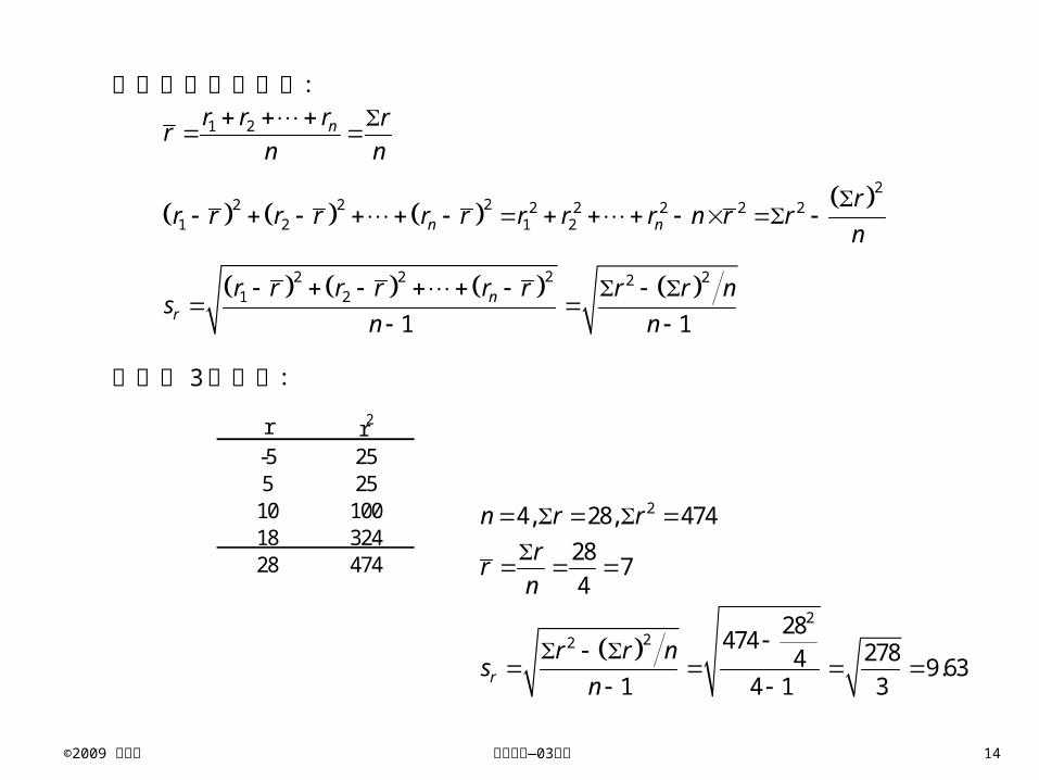
©2009 陳欣得 —03財務管理 風險 14
有關標準差的計算: 1 2 nr r r rr
n n
222 2 2 2 2 2 2
1 2 1 2n nr
r r r r r r r r r n r rn
22 2 221 2
1 1n
rr r r r r r r r n
sn n
如例題 3的計算:
r r2
-5 255 25
10 10018 32428 474
2
222
4, 28, 47428 74
28474 2784 9.631 4 1 3r
n r rrr
n
r r ns
n

©2009 陳欣得 —03財務管理 風險 15
第十章 風險與報酬:資本資產定價模式 10.1 報酬的期望值、變異數與共變數 10.2 兩資產組合的效率前緣 10.3 多項資產組合的風險 10.4 無風險借貸 10.5 決定資產風險 10.6 報酬與風險的關係

©2009 陳欣得 —03財務管理 風險 16
10.1 報酬的期望值、變異數與共變數 Rate of Return
Scenario Probability Stock fund Bond fundRecession 33.3% -7% 17%
Normal 33.3% 12% 7%Boom 33.3% 28% -3%
狀態 ( f )機率 股票(X) 債券(Y) Xf Yf X2f Y2f XYf衰退 1/3 -7% 17% -0.0233 0.0567 0.0016 0.0096 -0.0040持平 1/3 12% 7% 0.0400 0.0233 0.0048 0.0016 0.0028景氣 1/3 28% -3% 0.0933 -0.0100 0.0261 0.0003 -0.0028
0.1100 0.0700 0.0326 0.0116 -0.0040ΣX ΣY ΣX2 ΣY2 ΣXY
報酬率
11%X X 股票平均報酬 7%Y Y 債券平均報酬 22 2 20.0326 0.11 0.0205Xs X X 股票報酬變異數 22 2 20.0116 0.07 0.0067Ys Y Y 債券報酬變異數 22 14.3%Xs X X 22 8.2%Ys Y Y , 0.0040 0.11 0.07 0.0117X Ys XY X Y 股票與債券共變異數
, 0.0117 0.99500.1430 0.0820
X Y
X Y
ss s
股票與債券相關係數

©2009 陳欣得 —03財務管理 風險 17
股票與債券各佔 50%的投資組合:
Rate of ReturnScenario Stock fund Bond fund Portfolio squared deviationRecession -7% 17% 5.0% 0.160%Normal 12% 7% 9.5% 0.003%Boom 28% -3% 12.5% 0.123%
Expected return 11.00% 7.00% 9.0%Variance 0.0205 0.0067 0.0010Standard Deviation 14.31% 8.16% 3.08%

©2009 陳欣得 —03財務管理 風險 18
10.2 兩資產組合的效率前緣 % in stocks Risk Return
0% 8.2% 7.0%5% 7.0% 7.2%10% 5.9% 7.4%15% 4.8% 7.6%20% 3.7% 7.8%25% 2.6% 8.0%30% 1.4% 8.2%35% 0.4% 8.4%40% 0.9% 8.6%45% 2.0% 8.8%50% 3.1% 9.0%55% 4.2% 9.2%60% 5.3% 9.4%65% 6.4% 9.6%70% 7.6% 9.8%75% 8.7% 10.0%80% 9.8% 10.2%85% 10.9% 10.4%90% 12.1% 10.6%95% 13.2% 10.8%
100% 14.3% 11.0%
Portfolo Risk and Return Combinations
5.0%6.0%7.0%8.0%9.0%
10.0%11.0%12.0%
0.0% 2.0% 4.0% 6.0% 8.0% 10.0% 12.0% 14.0% 16.0%
Portfolio Risk (standard deviation)
Por
tfol
io R
etur
n

©2009 陳欣得 —03財務管理 風險 19
各種情況之兩資產組合:
100% bonds
retu
rn
100% stocks
= 0.2 = 1.0
= -1.0

©2009 陳欣得 —03財務管理 風險 20
10.3 項資產組合的風險
Nondiversifiable risk; Systematic Risk; Market Risk
Diversifiable Risk; Nonsystematic Risk; Firm Specific Risk; Unique Risk
n
Portfolio risk
兩類風險:
(1)可藉由投資組合分散的風險:可分散風險、非系統風險、廠商特有風險。
(2)無法藉由投資組合分散的風險:不可分散風險、系統風險、市場風險。
©2009 陳欣得 —03財務管理 風險 21
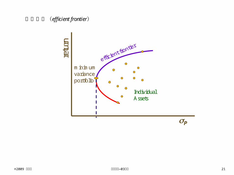
效率前緣(efficient frontier)
retu
rn
P
minimum variance portfolio
efficient frontier
Individual Assets

©2009 陳欣得 —03財務管理 風險 22
10.4 無風險借貸
各種組合與政府公債間的借貸方式
retu
rn
P
efficient frontier
rf
跨期借貸觀念

©2009 陳欣得 —03財務管理 風險 23
資本市場線(Capital Market Line, CML)
(風險 與報酬 r 為一直線關係。)
100% bonds
100% stocks
rf
retu
rn
Optimal Risky Portfolio

©2009 陳欣得 —03財務管理 風險 24
分離性質(The Separation Property)
分離性質(separation property):資本市場線(CML)的存在隱含以下性質
(1)所有人有共同的 CML與最適投資組合(M點)
(2)風險取向不同的投資者,會選擇在相同 CML上的不同位置

©2009 陳欣得 —03財務管理 風險 25
不同無風險資產決定不同資本市場線
100% bonds
100% stocksre
turn
First Optimal Risky Portfolio
Second Optimal Risky Portfolio
0fr
1fr
(下一階段:整合各種不同風險的資本市場線。)

©2009 陳欣得 —03財務管理 風險 26
10.5 決定資產風險
以市場最適投資組合為基礎來衡量個別資產的風險。
個別資產風險的測量值:
,2
( )( )
i Mi
M
Cov R RR
其中, MR 為市場最適投資組合的報酬率

©2009 陳欣得 —03財務管理 風險 27
以迴歸線決定 值
Secu
rity
Ret
urns
Secu
rity
Ret
urns
Return on Return on market %market %
RRii = = ii + + iiRRmm + + eeii
Slope = Slope = iiSlope = Slope = ii
(個別資產之報酬 ir 與市場報酬 Mr 間的關係。)

©2009 陳欣得 —03財務管理 風險 28
10.6 報酬與風險的關係
市場的期望報酬:
Market Risk PremiumM FR R
市場的期望報酬 無風險報酬 市場風險溢酬
個別資產的期望報酬:
β ( )i MF i FR R R R 市場風險溢酬

©2009 陳欣得 —03財務管理 風險 29
資本資產定價模式(Capital Asset Pricing Model, CAPM):
Expe
cted
retu
rn
)(β FMiFi RRRR
FR
1.0
MR

©2009 陳欣得 —03財務管理 風險 30
【例題】市場投資組合報酬為 10%,無風險報酬為 3%,某資產的 1.5 ,請以 CAPM
計算該資產的期望報酬。
【解】
3% 1.5 (10% 3%) 13.5%iR

©2009 陳欣得 —03財務管理 風險 31
第十一章 風險與報酬:套利定價理論

Slide 32
Copyright © 2008 by The McGraw-Hill Companies, Inc. All rights reserved
McGraw-Hill/Irwin
Arbitrage Pricing Theory
Arbitrage arises if an investor can construct a zero investment portfolio with a sure profit.
– Since no investment is required, an investor can create large positions to secure large levels of profit.
– In efficient markets, profitable arbitrage opportunities will quickly disappear.

©2009 陳欣得 —03財務管理 風險 33
套利定價理論(Arbitrage Pricing Theory) 若投資者可以建構一個零投入、有確定收益的投資組合, 則稱為存在套利機會。 若有套利機會,則該投資者可以創造極大的收益。 在效率市場,套利機會很快就會消失。

Slide 34
Copyright © 2008 by The McGraw-Hill Companies, Inc. All rights reserved
McGraw-Hill/Irwin
11.1 Factor Models: Announcements, Surprises, and Expected Returns
• The return on any security consists of two parts. – First, the expected returns– Second, the unexpected or risky returns
• A way to write the return on a stock in the coming month is:
return theofpart unexpected theis return theofpart expected theis
where
UR
URR

©2009 陳欣得 —03財務管理 風險 35
因素模型(Factor Models) 投資的報酬分為兩部分:可預期報酬與不可預期報酬。 R R U

Slide 36
Copyright © 2008 by The McGraw-Hill Companies, Inc. All rights reserved
McGraw-Hill/Irwin
Risk: Systematic and Unsystematic
Systematic Risk: m
Nonsystematic Risk:
n
2
Total risk
We can break down the total risk of holding a stock into two components: systematic risk and unsystematic risk:
becomes
where is
is
R R U
R R m ε
mε
系統風險非系統風險

Slide 37
Copyright © 2008 by The McGraw-Hill Companies, Inc. All rights reserved
McGraw-Hill/Irwin
Systematic Risk and Betas• For example, suppose we have identified
three systematic risks: inflation, GNP growth, and the dollar-euro spot exchange rate, S($,€).
• Our model is:
is the inflation beta is the GNP beta
is the spot exchange rate beta is the unsystematic risk
I I GNP GNP S S
I
GNP
S
R R m ε
R R β F β F β F εβββε
(通貨膨脹)
(匯兌)

Slide 38
Copyright © 2008 by The McGraw-Hill Companies, Inc. All rights reserved
McGraw-Hill/Irwin
Systematic Risk and Betas: Example
• Suppose we have made the following estimates:1. I = -2.30
2. GNP = 1.50
3. S = 0.50• Finally, the firm was able to attract a “superstar” CEO,
and this unanticipated development contributes 1% to the return.
εFβFβFβRR SSGNPGNPII
%1ε
%150.050.130.2 SGNPI FFFRR

Slide 39
Copyright © 2008 by The McGraw-Hill Companies, Inc. All rights reserved
McGraw-Hill/Irwin
Systematic Risk and Betas: Example
We must decide what surprises took place in the systematic factors.
If it were the case that the inflation rate was expected to be 3%, but in fact was 8% during the time period, then:
FI = Surprise in the inflation rate = actual – expected
= 8% – 3% = 5%
%150.050.130.2 SGNPI FFFRR
%150.050.1%530.2 SGNP FFRR

Slide 40
Copyright © 2008 by The McGraw-Hill Companies, Inc. All rights reserved
McGraw-Hill/Irwin
Systematic Risk and Betas: Example
If it were the case that the rate of GNP growth was expected to be 4%, but in fact was 1%, then:
FGNP = Surprise in the rate of GNP growth
= actual – expected = 1% – 4% = – 3%
%150.050.1%530.2 SGNP FFRR
%150.0%)3(50.1%530.2 SFRR

Slide 41
Copyright © 2008 by The McGraw-Hill Companies, Inc. All rights reserved
McGraw-Hill/Irwin
Systematic Risk and Betas: Example
If it were the case that the dollar-euro spot exchange rate, S($,€), was expected to increase by 10%, but in fact remained stable during the time period, then:
FS = Surprise in the exchange rate
= actual – expected = 0% – 10% = – 10%
%150.0%)3(50.1%530.2 SFRR
%1%)10(50.0%)3(50.1%530.2 RR

Slide 42
Copyright © 2008 by The McGraw-Hill Companies, Inc. All rights reserved
McGraw-Hill/Irwin
Systematic Risk and Betas: Example
Finally, if it were the case that the expected return on the stock was 8%, then:
%1%)10(50.0%)3(50.1%530.2 RR
%12%1%)10(50.0%)3(50.1%530.2%8
RR
%8R

Slide 43
Copyright © 2008 by The McGraw-Hill Companies, Inc. All rights reserved
McGraw-Hill/Irwin
11.6 CAMP 與 APT
• APT applies to well diversified portfolios and not necessarily to individual stocks.
• With APT it is possible for some individual stocks to be mispriced - not lie on the SML.
• APT is more general in that it gets to an expected return and beta relationship without the assumption of the market portfolio.
• APT can be extended to multifactor models.

Slide 44
Copyright © 2008 by The McGraw-Hill Companies, Inc. All rights reserved
McGraw-Hill/Irwin
11.7 Empirical Approaches to Asset Pricing
• Both the CAPM and APT are risk-based models. • Empirical methods are based less on theory and
more on looking for some regularities in the historical record.
• Be aware that correlation does not imply causality.• Related to empirical methods is the practice of
classifying portfolios by style, e.g.,– Value portfolio– Growth portfolio

©2009 陳欣得 —03財務管理 風險 45
第十二章 風險、資金成本與資本預算 12.1 權益成本 12.2 估計 Beta 值 12.3 影響 Beta 值的因素 12.4 基本權益成本估計模型之延伸 12.5 降低資金成本

©2009 陳欣得 —03財務管理 風險 46
12.1 權益成本
公司剩餘資金的投資報酬率應高於股東個人的投資報酬率。
Invest in projectInvest in project
Firm withexcess cash
Shareholder’s Terminal
Value
Pay cash dividendPay cash dividend
Shareholder invests in financial
asset
A firm with excess cash can either pay a dividend or make a capital investment
資本資產定價模式(CAPM)是一個估計權益成本方法:
( )i MF i FR R β R R
其中需先知道: FR 為無風險報酬率、 M FR R 為市場的風險溢酬、公司的 i 值。

©2009 陳欣得 —03財務管理 風險 47
【例題】Suppose the stock of Stansfield Enterprises, a publisher of PowerPoint
presentations, has a beta of 2.5. The firm is 100-percent equity financed.
Assume a risk-free rate of 5-percent and a market risk premium of 10-percent.
What is the appropriate discount rate for an expansion of this firm?
【解】
已知: 2.5i 、 5%FR 、 10%M FR R ,
( ) 5% 2.5 10% 30%i MF i FR R β R R

©2009 陳欣得 —03財務管理 風險 48
利用證券市場線(SML)評估專案的優劣:
Proj
ect
IRR
Firm’s risk (beta)
SML
5%
Good project
Bad project
30%
2.5
A
B
C
30%
2.5
A
B
C
©2009 陳欣得 —03財務管理 風險 49
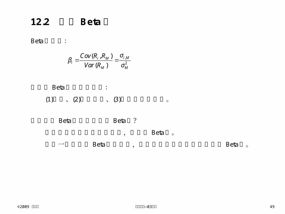
12.2 估計 Beta值
Beta的公式:
,2
( , )( )
i Mi Mi
M M
σCov R Rβ
Var R σ
會影響 Beta估計值的因素:
(1)時間、(2)樣本大小、(3)融資與風險狀況。
使用產業 Beta值或個別公司 Beta值?
若公司與產業平均狀況同質,用產業 Beta值。
雖然一個公司的 Beta值很穩定,但是不同投資專案應該有不同 Beta值。

©2009 陳欣得 —03財務管理 風險 50
【例題】某 g公司與其產業在過去四年的報酬資料如下,請計算 g公司的 Beta值。
年度 Rg RM
1 -10% -40%2 3% -30%3 20% 10%4 15% 20%
【解】
計算草稿與過程如下:
年度 Rg RM RM2 Rg×RM
1 -10% -40% 0.1600 0.04002 3% -30% 0.0900 -0.00903 20% 10% 0.0100 0.02004 15% 20% 0.0400 0.0300合計 0.2800 -0.4000 0.3000 0.0810
ΣRg ΣRM ΣRM2 Σ(Rg×RM)
22 0.30 0.40 4
0.08674 1M
,
0.081 0.28 0.40 40.0363
4 1g M
,2
( , ) 0.0363 0.42( ) 0.0867
g M g Mg
M M
Cov R R σβ
Var R σ

©2009 陳欣得 —03財務管理 風險 51
12.3 影響 Beta值的因素
討論三個影響 Beta值的因素:
經營風險: (1)收益週期循環性(Cyclicity of Revenues)
(2)營運槓稈(Operating Leverage)
財務風險: (3)財務槓桿(Financial Leverage)
收益週期循環性(Cyclicity of Revenues)
一般高循環性的股票有較高的報酬。
高循環性並不意味著高變異性。

©2009 陳欣得 —03財務管理 風險 52
營運槓稈(Operating Leverage):衡量固定成本對營收得影響。
固定成本增加會增加營運槓桿,反之,變動成本增加則減少營運槓桿。
營運槓桿會擴大收益的循環變動。
衡量營運槓桿(Degree of Operating Leverage,DOL):
EBITEBITDOLSales
Sales
Volume
$
Fixed costs
Total costs
EBIT
VolumeFixed costsFixed costs
Total costsTotal costs

©2009 陳欣得 —03財務管理 風險 53
財務槓桿(Financial Leverage):衡量固定資金成本對營收得影響。
Asset Debt EquityDebt Equity
Debt Equity Debt Equity
資產 負債 權益
負債 權益負債 權益 負債 權益
©2009 陳欣得 —03財務管理 風險 54
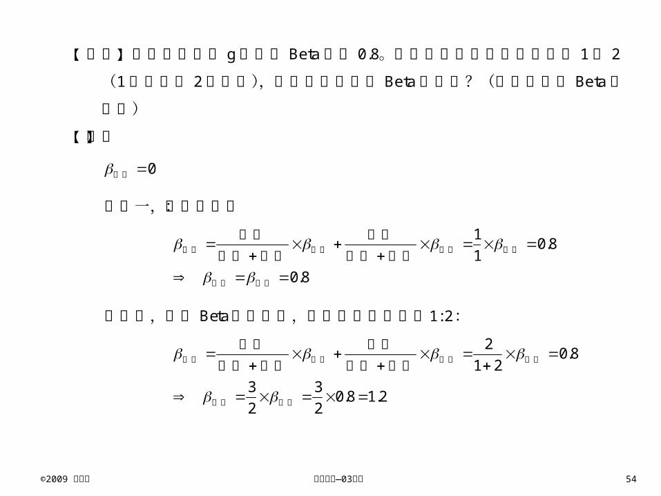
【例題】某全部權益的 g公司之 Beta值為 0.8。若該公司將財務槓桿調整為 1比 2
(1份負債比 2份權益),則該公司權益的 Beta值為何?(假設負債的 Beta值
為零)
【解】
0 負債
狀況一,全部權益:
1 0.81
0.8
資產 負債 權益 權益
資產 權益
負債 權益負債 權益 負債 權益
狀況二,資產 Beta值不變下,負債權益比調整為1: 2:
2 0.81 2
3 3 0.8 1.22 2
資產 負債 權益 權益
權益 資產
負債 權益負債 權益 負債 權益

©2009 陳欣得 —03財務管理 風險 55
12.4 基本權益成本估計模型之延伸
公司風險與專案風險
專案的資金成本與該資金的用途(use)有關,而與該資金的來源(source)無關。
因此,資金成本應以專案的風險為評估依據,而不是以公司的風險為依據。 Pr
ojec
t IR
R
Firm’s risk (beta)
SML
rfrf
FIRMFIRM
Incorrectly rejected positive NPV projectsIncorrectly rejected positive NPV projects
Incorrectly accepted negative NPV projectsIncorrectly accepted negative NPV projects
Hurdle rate
)( FMFIRMF RRβR
The SML can tell us why:

©2009 陳欣得 —03財務管理 風險 56
加權平均資金成本(Weighted Average Cost of Capital,WACC)
1WACC S B CS Br r r T
B S B S
其中: S權益總金額、 Sr 權益報酬率、B負債總金額、 Br 負債利息、 CT 公司稅
率 S F M Fr R R R

©2009 陳欣得 —03財務管理 風險 57
【例題】某公司負債的市值為 4000萬,權益的市值為 6000萬。該公司給付負債 15%
的利息,且該公司的 Beta值等於 1.41,適用稅率為 34%。若無風險利率為 11%,
市場的風險溢酬為 9.5%,請計算該公司的加權平均資金成本。
【解】
基本資料: 4000B 、 6000S 、 15%Br 、 1.41 、 34%CT 、 11%FR
11% 1.41 9.5% 24.40%S F M Fr R R R
6000 400024.40% 15% 1 0.34 18.60%4000 6000 4000 6000WACCr

©2009 陳欣得 —03財務管理 風險 58
12.5 降低資金成本
流動性(Liquidity):資產、有價證券的變現能力。
變現能力有兩個層面:(1)變現時間、(2)變現成本。
流動性與資金成本的關係:
Cos
t of C
apita
l
Liquidity

©2009 陳欣得 —03財務管理 風險 59
請就下列資料回答 5、6、7三題:
弘海公司有閒餘資金新台幣 1億元,將分散投資於高科技產業(30%)與傳統產
業(70%)。投資時預期之景氣狀態與報酬率資料如下表:
景氣狀態 發生機率 高科技預期報酬 傳統產業預期報酬蕭條 0.2 -3% 4%一般 0.5 10% 6%繁榮 0.3 18% 8%
5. 該公司預期之投資組合報酬為何? 6. 該公司之投資組合之風險為何? 7. 若想要讓投資組合風險最低,則投資於高科技產業的權重(比例)應為何?
【解】
景氣狀態 發生機率 投資組合報酬 Xf X2f蕭條 0.2 1.90% 0.0038 0.000072一般 0.5 7.20% 0.0360 0.002592繁榮 0.3 11.00% 0.0330 0.003630
0.0728 0.006294 E X 7.28%
22 20.006294 0.0728E X E X 3.15%

©2009 陳欣得 —03財務管理 風險 60
8. A公司的平均報酬率為 20%,標準差 8%;市場的平均報酬率為 12%,標準差 6%。若 A公司與市場報酬率的相關係數為 0.8,請計算 A公司的 beta值。
【解】
,8%, 6%, 0.8B M B M
20.8 8%
6%AM AM A
AMM
1.07

©2009 陳欣得 —03財務管理 風險 61
請就下列資料回答 9、10、11三題:
假設 B公司之β 值為 1.5,市場投資組合之平均報酬率為 12%,無風險利率為 4%,且稅率為 30%。此公司之資本結構為負債與業主權益分別占 40%與 60%,其中負債的利率為 9%。
9. 該公司的權益成本( Sr )為為何? 10. 該公司的實質(稅後)負債成本為何? 11. 該公司的加權資金成本( WACCr )為為何?
【解】
4% 1.5 12% 4%S f M fr r r r 16%
1 9% 1 30%B Cr T 6.3%
60 401 16% 6.3%100 100WACC S B C
S Br r r TB S B S
12.12%

©2009 陳欣得 —03財務管理 風險 62
結束 Part III