2. Pooled Cross Sections and Panels Pooled Cross Sections ...lipas.uwasa.fi/~bepa/Panels.pdf · Pooled Cross Sections and Panels 2.1 Pooled Cross Sections versus Panel Data Pooled

2. Pooled Cross Sections and Panels

2.1 Pooled Cross Sections versus Panel Data

Pooled Cross Sections are obtained by col-

lecting random samples from a large polula-

tion independently of each other at different

points in time. The fact that the random

samples are collected independently of each

other implies that they need not be of equal

size and will usually contain different statis-

tical units at different points in time.

Consequently, serial correlation of residuals

is not an issue, when regression analysis is

applied. The data can be pretty much an-

alyzed like ordinary cross-sectional data, ex-

cept that we must use dummies in order to

account for shifts in the distribution between

different points in time.

1

Panel Data or longitudinal data consists of

time series for each statistical unit in the

cross section. In other words, we randomly

select our cross section only once, and once

that is done, we follow each statistical unit

within this cross section over time. Thus all

cross sections are equally large and consist of

the same statistical units.

For panel data we cannot assume that the

observations are independently distributed

across time and serial correlation of regres-

sion residuals becomes an issue. We must

be prepared that unobserved factors, while

acting differently on different cross-sectional

units, may have a lasting effect upon the

same statistical unit when followed through

time. This makes the statistical analysis of

panel data more difficult.

2

2.2 Independent Pooled Cross Sections

Example 1: Women’s fertility over time.

Regressing the number of children born per

woman upon year dummies and controls such

as education, age etc. yields information about

the development of fertility unexplained by

the controls. (Base year 1972)

Dependent Variable: KIDSMethod: Least SquaresDate: 11/23/12 Time: 08:21Sample: 1 1129Included observations: 1129

Variable Coefficient Std. Error t-Statistic Prob.

C -7.742457 3.051767 -2.537040 0.0113EDUC -0.128427 0.018349 -6.999272 0.0000AGE 0.532135 0.138386 3.845283 0.0001

AGESQ -0.005804 0.001564 -3.710324 0.0002BLACK 1.075658 0.173536 6.198484 0.0000EAST 0.217324 0.132788 1.636626 0.1020

NORTHCEN 0.363114 0.120897 3.003501 0.0027WEST 0.197603 0.166913 1.183867 0.2367FARM -0.052557 0.147190 -0.357072 0.7211

OTHRURAL -0.162854 0.175442 -0.928248 0.3535TOWN 0.084353 0.124531 0.677367 0.4983

SMCITY 0.211879 0.160296 1.321799 0.1865Y74 0.268183 0.172716 1.552737 0.1208Y76 -0.097379 0.179046 -0.543881 0.5866Y78 -0.068666 0.181684 -0.377945 0.7055Y80 -0.071305 0.182771 -0.390136 0.6965Y82 -0.522484 0.172436 -3.030016 0.0025Y84 -0.545166 0.174516 -3.123871 0.0018

R-squared 0.129512 Mean dependent var 2.743136Adjusted R-squared 0.116192 S.D. dependent var 1.653899S.E. of regression 1.554847 Akaike info criterion 3.736447Sum squared resid 2685.898 Schwarz criterion 3.816627Log likelihood -2091.224 Hannan-Quinn criter. 3.766741F-statistic 9.723282 Durbin-Watson stat 2.010694Prob(F-statistic) 0.000000

3

We can also interact a time dummy with key

explanatory variables to see if the effect of

that variable has changed over time.

Example 2:

Changes in the return to education and the

gender wage gap between 1978 and 1985.

Dependent Variable: LWAGEMethod: Least SquaresDate: 11/27/12 Time: 17:25Sample: 1 1084Included observations: 1084


C 0.458933 0.093449 4.911078 0.0000EXPER 0.029584 0.003567 8.293165 0.0000

EXPER^2 -0.000399 7.75E-05 -5.151307 0.0000UNION 0.202132 0.030294 6.672233 0.0000EDUC 0.074721 0.006676 11.19174 0.0000

FEMALE -0.316709 0.036621 -8.648173 0.0000Y85 0.117806 0.123782 0.951725 0.3415

Y85*EDUC 0.018461 0.009354 1.973509 0.0487Y85*FEMALE 0.085052 0.051309 1.657644 0.0977


The return to education has risen by about

1.85% and the gender wage gap narrowed by

about 8.5% between 1978 and 1985, other

factors being equal.

4

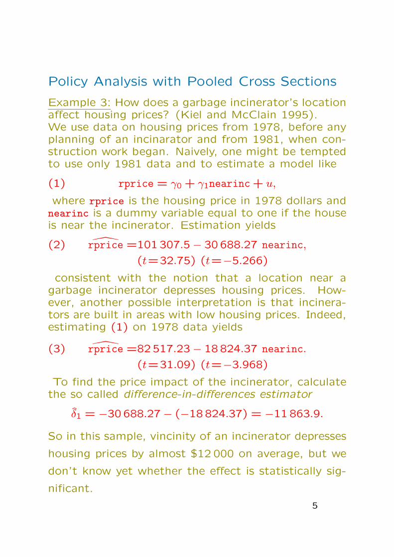
Policy Analysis with Pooled Cross Sections

Example 3: How does a garbage incinerator’s locationaffect housing prices? (Kiel and McClain 1995).We use data on housing prices from 1978, before anyplanning of an incinarator and from 1981, when con-struction work began. Naively, one might be temptedto use only 1981 data and to estimate a model like

(1) rprice = γ0 + γ1nearinc + u,

where rprice is the housing price in 1978 dollars andnearinc is a dummy variable equal to one if the houseis near the incinerator. Estimation yields

rprice =101 307.5− 30 688.27 nearinc,(2)

(t=32.75) (t=−5.266)

consistent with the notion that a location near agarbage incinerator depresses housing prices. How-ever, another possible interpretation is that incinera-tors are built in areas with low housing prices. Indeed,estimating (1) on 1978 data yields

rprice =82 517.23− 18 824.37 nearinc.(3)

(t=31.09) (t=−3.968)

To find the price impact of the incinerator, calculatethe so called difference-in-differences estimator

δ1 = −30 688.27− (−18 824.37) = −11 863.9.

So in this sample, vincinity of an incinerator depresses

housing prices by almost $12 000 on average, but we

don’t know yet whether the effect is statistically sig-

nificant.

5

The previous example is called a natural ex-periment (or a quasi-experiment). It occurswhen some external event (often a policychange) affects some group, called the treat-ment group, but leaves another group, calledthe control group, unaffected. It differs froma true experiment in that these groups arenot randomly and explicitely chosen.

Let DT be a dummy variable indicating whetheran observation is from the treatment groupand Dafter be a dummy variable indicatingwhether the observation is from after the ex-ogeneous event. Then the impact of the ex-ternal event on y is given by δ1 in the model

y =β0 + δ0Dafter + β1DT + δ1Dafter ·DT(4)

(+other factors).

If no other factors are included, δ1 will bethe difference-in-differences estimator

(5) δ1 = (yafter,T − ybef.,T )− (yafter,C − ybef.,C),

where T and C denote the treatment andcontrol group, respectively.

6

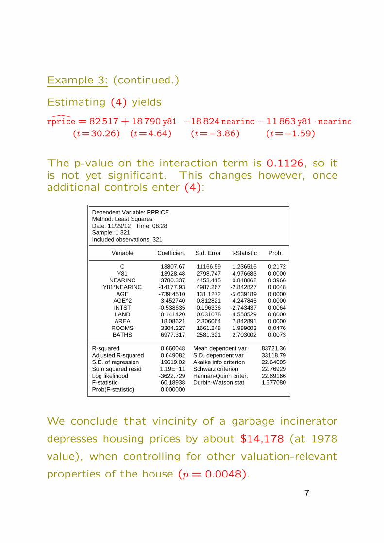
Example 3: (continued.)

Estimating (4) yields

rprice = 82 517 + 18 790 y81 −18 824 nearinc− 11 863 y81 · nearinc(t=30.26) (t=4.64) (t=−3.86) (t=−1.59)

The p-value on the interaction term is 0.1126, so itis not yet significant. This changes however, onceadditional controls enter (4):

Dependent Variable: RPRICEMethod: Least SquaresDate: 11/29/12 Time: 08:28Sample: 1 321Included observations: 321


C 13807.67 11166.59 1.236515 0.2172Y81 13928.48 2798.747 4.976683 0.0000

NEARINC 3780.337 4453.415 0.848862 0.3966Y81*NEARINC -14177.93 4987.267 -2.842827 0.0048

AGE -739.4510 131.1272 -5.639189 0.0000AGE^2 3.452740 0.812821 4.247845 0.0000INTST -0.538635 0.196336 -2.743437 0.0064LAND 0.141420 0.031078 4.550529 0.0000AREA 18.08621 2.306064 7.842891 0.0000

ROOMS 3304.227 1661.248 1.989003 0.0476BATHS 6977.317 2581.321 2.703002 0.0073

R-squared 0.660048 Mean dependent var 83721.36Adjusted R-squared 0.649082 S.D. dependent var 33118.79S.E. of regression 19619.02 Akaike info criterion 22.64005Sum squared resid 1.19E+11 Schwarz criterion 22.76929Log likelihood -3622.729 Hannan-Quinn criter. 22.69166F-statistic 60.18938 Durbin-Watson stat 1.677080Prob(F-statistic) 0.000000

We conclude that vincinity of a garbage incinerator

depresses housing prices by about $14,178 (at 1978

value), when controlling for other valuation-relevant

properties of the house (p = 0.0048).

7

2.3 First-Difference Estimation in Panels

Recall from Econometrics 1 that omitting

important variables in the model may induce

severe bias to all parameter estimates. This

was called the omitted variable bias. Panel

data allows to mitigate, if not eliminate, this

problem.

Example 4.Crime and unemployment rates for 46 cities in 1982and 1987. Regressing the crimerate (crimes per 1 000people) crmte upon the unemployment rate unem (inpercent) yields for the 1987 cross section

crmrte = 128.38 − 4.16unem.

(t=6.18) (t=−1.22)

Even though unemployment is nonsignificant (p=0.23),

a causal interpretation would imply that an increase

in unemployment lowers the crime rate, which is hard

to believe. The model probably suffers from omitted

variable bias.

8

With panel data we view the unobserved fac-tors affecting the dependent variable as con-sisting of two types: those that are constantand those that vary over time. Letting i de-note the cross-sectional unit and t time:

(6) yit = β0 + δ0D2,t + β1xit + ai + uit. t=1,2

The dummy variable D2,t is zero for t = 1

and one for t = 2. It models the time-varying

part of the unobserved factors. The variable

ai captures all unobserved, time-constant fac-

tors that affect yit. ai is generally called an

unobserved or fixed effect. uit is called the

idiosyncratic error. A model of the form (6)

is called an unobserved effects model or fixed

effects model.

Example 4 (continued). A fixed effects modelfor city crime rates in 1982 and 1987 is

(7) crmrteit = β0 + δ0D87,t + β1unemit + ai + uit,

where D87 is dummy variable for 1987.

9

Naively, we might go and estimate a fixed

effects model by pooled OLS. That is, we

write (6) in the form

(8) yit = β0 + δ0D2,t + β1xit + νit, t=1,2,

and apply OLS, where νit = ai + uit is called

the composite error.

Such an approach is problematic for two rea-

sons. As a minor complication it turns out

that Cov(νi1, νi2) = V (ai) even though ai and

uit are pairwise uncorrelated, such that the

composite errors become positively correlated

over time. This problem is minor because it

can be solved by using standard errors which

are robust to serial correlation in the residu-

als (HAC (Newey-West) resp. White period

robust standard errors in EViews).

10

The main problem with applying pooled OLS

is that we did very little to solve the omitted

variable bias problem. Only the time-varying

part (assumed to be common for all cross-

sesctional units) has been taken out by in-

troducing the time dummy. The fixed effect

ai, however, is still there; it has just been hid-

den in the composite error νit, and is there-

fore not modeled. That is, the parameter

estimates are still biased, unless ai is uncor-

related with xit.

Example 4 (continued).

Pooled OLS on the crime rate data yields

(9) crmrte = 93.42 + 7.94D87 + 0.427unem.

The (wrong) p-value using OLS standard er-

rors is 0.721, and applying Newey and West

(1987) HAC standard errors p = 0.693. Thus,

while the unemployment rate has now the ex-

pected sign, it is still deemed nonsignificant.

11

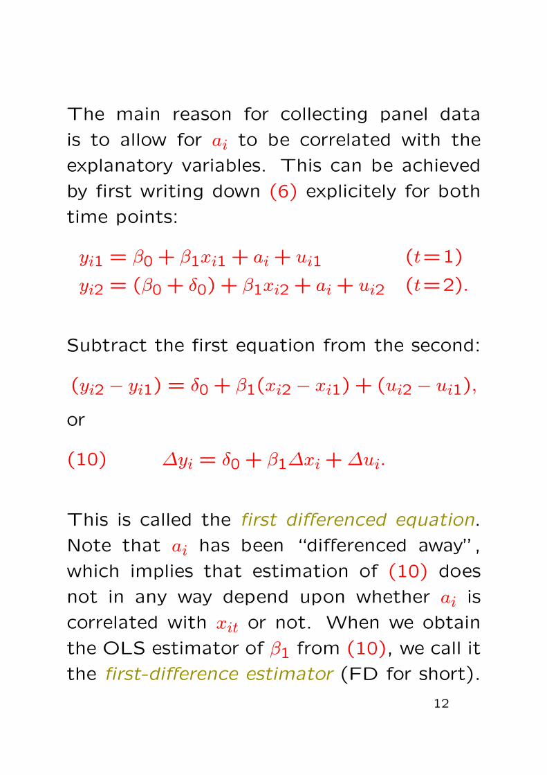
The main reason for collecting panel data

is to allow for ai to be correlated with the

explanatory variables. This can be achieved

by first writing down (6) explicitely for both

time points:

yi1 = β0 + β1xi1 + ai + ui1 (t=1)

yi2 = (β0 + δ0) + β1xi2 + ai + ui2 (t=2).

Subtract the first equation from the second:

(yi2 − yi1) = δ0 + β1(xi2 − xi1) + (ui2 − ui1),

or

(10) ∆yi = δ0 + β1∆xi +∆ui.

This is called the first differenced equation.

Note that ai has been “differenced away”,

which implies that estimation of (10) does

not in any way depend upon whether ai is

correlated with xit or not. When we obtain

the OLS estimator of β1 from (10), we call it

the first-difference estimator (FD for short).

12

The parameters of (10) can be consistentlyestimated by OLS when the classical assump-tions for regression analysis hold.

In particular, ∆ui must be uncorrelated with∆xi, which holds if uit is uncorrelated withxit in both time periods. That is, we needstrict exogeneity. In particular, this rules outincluding lagged dependent variables such asyi,t−1 as explanatory variables. Lagged in-dependent variables such as xi,t−1 may beincluded without problems.

Another crucial assumption is that there mustbe variation in ∆xi. This rules out indepen-dent variables which do not change over timeor change by the same amount for all cross-sectional units.

Example 4 (continued).

Estimation of (10) yields

∆crmrte = 15.40 + 2.22∆unem,

(t=3.28) (t=2.52)

which now gives a positive, statistically significant

relationship (p = 0.015) between unemployment and

crime rates.

13

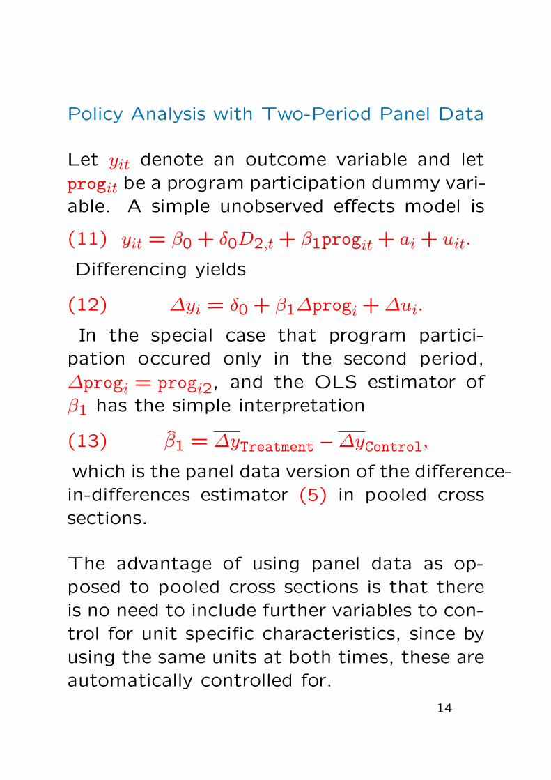
Policy Analysis with Two-Period Panel Data

Let yit denote an outcome variable and letprogit be a program participation dummy vari-able. A simple unobserved effects model is

(11) yit = β0 + δ0D2,t + β1progit + ai + uit.

Differencing yields

(12) ∆yi = δ0 + β1∆progi +∆ui.

In the special case that program partici-pation occured only in the second period,∆progi = progi2, and the OLS estimator ofβ1 has the simple interpretation

(13) β1 = ∆yTreatment −∆yControl,which is the panel data version of the difference-in-differences estimator (5) in pooled crosssections.

The advantage of using panel data as op-posed to pooled cross sections is that thereis no need to include further variables to con-trol for unit specific characteristics, since byusing the same units at both times, these areautomatically controlled for.

14

Example 5.Job training program on worker productivity.

Let scrapit denote the scrap rate of firm iduring year t, and let grantit be a dummyequal to one if firm i received a job traininggrant in year t. Pooled OLS yields using datafrom the years 1987 and 1988

log(scrapit) = 0.5974 − 0.1889D88 + 0.0566grant,

(p=0.005) (p=0.566) (p=0.896)

suggesting that grants increase scrap rates.The preceding model suffers most likely fromomitted variables bias. Estimating the firstdifferenced equation (12) instead yields

∆ log(scrap) = − 0.057 − 0.317∆grant.

(p=0.557) (p=0.059)

Having a job training grant is estimated tolower the scrap rate by about 27.2%, sinceexp(−0.317)− 1 ≈ −0.272. The effect is sig-nificant at 10% but not at 5%. The largedifference between β1 obtained from pooledOLS and applying the first differenced esti-mator suggests that grants were mainly placedto firms which produce poorer quality.No further variables (controls) with possibleimpact upon scrap rates need to be includedin the model.

15

Differencing with More Than 2 Periods

The fixed effects model in the general casewith k regressors and T time periods is

yit =δ1 + δ2D2,t + · · ·+ δTDT,t(14)

+k∑

j=1

βjxtij + ai + uit,

The key assumption is that the idiosyncraticerrors are uncorrelated with the explanatoryvariables at all times (strict exogeneity):

(15) Cov(xitj, uis) = 0 for all t, s and j,

which rules out using lagged dependent vari-ables as regressors. Differencing(14) yields

∆yit =δ2∆D2,t + · · ·+ δT∆DT,t(16)

+k∑

j=1

βj∆xtij +∆uit

for t = 2, . . . , T . Note that both the intercept δ1 and

the unobservable effect ai have disappeared. This im-

plies that while possible correlations between ai and

any of the explanatory variables causes omitted vari-

ables bias in (14), it causes no problem in estimating

the first differenced equation (16).

16

Example 6.Enterprise Zones and Unemployment Claims

Unemployment claims uclms in 22 cities from 1980 to1988 as a function of whether the city has an enter-prise zone (ez = 1) or not:

log(uclmsit) = θt + β1ezit + ai + uit,

where θt shifts the intercept with appropriate yeardummies. FD estimation output:

Dependent Variable: D(LUCLMS)Method: Panel Least SquaresDate: 11/29/12 Time: 16:45Sample (adjusted): 1981 1988Periods included: 8Cross-sections included: 22Total panel (balanced) observations: 176


D81 -0.321632 0.046064 -6.982279 0.0000D82 0.457128 0.046064 9.923744 0.0000D83 -0.354751 0.046064 -7.701262 0.0000D84 -0.338770 0.050760 -6.673948 0.0000D85 0.001449 0.048208 0.030058 0.9761D86 -0.029478 0.046064 -0.639934 0.5231D87 -0.267684 0.046064 -5.811126 0.0000D88 -0.338684 0.046064 -7.352471 0.0000

D(EZ) -0.181878 0.078186 -2.326211 0.0212

R-squared 0.622997 Mean dependent var -0.159387Adjusted R-squared 0.604937 S.D. dependent var 0.343748S.E. of regression 0.216059 Akaike info criterion -0.176744Sum squared resid 7.795839 Schwarz criterion -0.014617Log likelihood 24.55348 Hannan-Quinn criter. -0.110986Durbin-Watson stat 2.441511

The presence of an enterprise zone appears to reduce

unemployment claims by about 18% (p = 0.0212).

Note that we have replaced the change in year dummies ∆D in

(16) with the year dummies themselves. This can be shown to

have no effect on the other parameter estimates (here D(EZ)).

17

2.4 Dummy Variable Regression in Panels

Another way to eliminate possible correla-tions with the unobservable factors ai in (14)is to model them explicitly as dummy vari-ables, where each cross-sectional unit getsits own dummy. This may be written as

(17) y = Xβ + Zµ+ u, where

for N cross sections and T time periods:y is a (NT ×1) vector of observations on yit,X is a (NT × k) matrix of regressors xitj,β is a (k × 1) vector of slope parameters βj,Z is a (NT ×N) matrix of dummies,µ is a (N×1) vector of unobservables ai, andu is a (NT × 1) vector of error terms uit.

It is customs to stack y,X,Z and u such thatthe slower index is over cross sections i, andthe faster index is over time points t, e.g.

y′ = (y11, . . . , y1T , . . . , yN1, . . . , yNT ).

Note that there is no constant in (17) in or-der to avoid exact multicollinearity (dummyvariable trap). If you wish to include a con-stant, use only N−1 dummy variables for theN cross-sectional units.

18

Example 6. (continued)Regressing log(uclms) on the year dummies,22 dummies for the cities in sample and theenterprise zone dummy ez yields

Dependent Variable: LUCLMSMethod: Panel Least SquaresDate: 12/04/12 Time: 10:39Sample: 1980 1988Periods included: 9Cross-sections included: 22Total panel (balanced) observations: 198


D81 -0.321632 0.060457 -5.319980 0.0000D82 0.135496 0.060457 2.241179 0.0263D83 -0.219255 0.060457 -3.626613 0.0004D84 -0.579152 0.062318 -9.293490 0.0000D85 -0.591787 0.065495 -9.035540 0.0000D86 -0.621265 0.065495 -9.485616 0.0000D87 -0.888949 0.065495 -13.57268 0.0000D88 -1.227633 0.065495 -18.74379 0.0000C1 11.67615 0.080079 145.8073 0.0000C2 11.48266 0.079105 145.1574 0.0000C3 11.29721 0.079105 142.8131 0.0000C4 11.13498 0.079105 140.7621 0.0000C5 11.68718 0.078930 148.0695 0.0000C6 12.23073 0.080079 152.7326 0.0000C7 12.42622 0.080079 155.1738 0.0000C8 11.61739 0.078930 147.1852 0.0000C9 12.02958 0.078930 152.4074 0.0000

C10 13.32116 0.079105 168.3987 0.0000C11 11.54584 0.079105 145.9560 0.0000C12 11.64117 0.079105 147.1612 0.0000C13 10.84358 0.079105 137.0784 0.0000C14 10.80252 0.078930 136.8613 0.0000C15 11.44073 0.079105 144.6273 0.0000C16 12.11190 0.079105 153.1118 0.0000C17 11.23093 0.080079 140.2475 0.0000C18 11.63326 0.079105 147.0611 0.0000C19 11.76956 0.079105 148.7842 0.0000C20 11.32518 0.080079 141.4244 0.0000C21 12.13394 0.080079 151.5240 0.0000C22 11.89479 0.079105 150.3673 0.0000EZ -0.104415 0.055419 -1.884091 0.0613

R-squared 0.933188 Mean dependent var 11.19078Adjusted R-squared 0.921185 S.D. dependent var 0.714236S.E. of regression 0.200514 Akaike info criterion -0.233004Sum squared resid 6.714401 Schwarz criterion 0.281826Log likelihood 54.06741 Hannan-Quinn criter. -0.024618Durbin-Watson stat 1.306450

(marginally significant decrease by 10%.)

19

2.5 Fixed Effects (FE) Estimation in Panels

Dummy variable regressions become imprac-

tical when the number of cross-sections gets

large. An alternative method, which turns

out to yield identical results, is called the

fixed effects method.

As an example consider the simple model

(18) yit = β1xit + ai + uit,

i = 1, . . . , N , t = 1, . . . , T .

Thus there are altogether N × T observations.

Define means over the T time periods

(19) yi =1

T

T∑t=1

yit, xi =1

T

T∑t=1

xit, ui =1

T

T∑t=1

uit.

Then averaging over T yields

(20) yi = β1xi + ai + ui,

since

1

T

T∑t=1

ai =1

TTai = ai.

20

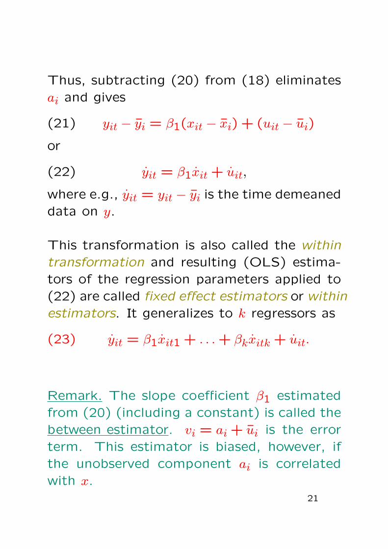
Thus, subtracting (20) from (18) eliminatesai and gives

(21) yit − yi = β1(xit − xi) + (uit − ui)

or

(22) yit = β1xit + uit,

where e.g., yit = yit − yi is the time demeaneddata on y.

This transformation is also called the withintransformation and resulting (OLS) estima-tors of the regression parameters applied to(22) are called fixed effect estimators or withinestimators. It generalizes to k regressors as

(23) yit = β1xit1 + . . .+ βkxitk + uit.

Remark. The slope coefficient β1 estimatedfrom (20) (including a constant) is called thebetween estimator. vi = ai + ui is the errorterm. This estimator is biased, however, ifthe unobserved component ai is correlatedwith x.

21

Example 6. (continued)Regressing the differences of log(uclms) fromtheir means upon the differences of the yeardummies from their means and the differ-ences of the enterprize zone dummy ez fromits means yields

Dependent Variable: LUCLMS-MLUCLMSMethod: Panel Least SquaresDate: 12/04/12 Time: 13:09Sample: 1980 1988Periods included: 9Cross-sections included: 22Total panel (balanced) observations: 198


D81-MD81 -0.321632 0.056830 -5.659560 0.0000D82-MD82 0.135496 0.056830 2.384236 0.0181D83-MD83 -0.219255 0.056830 -3.858104 0.0002D84-MD84 -0.579152 0.058579 -9.886703 0.0000D85-MD85 -0.591787 0.061566 -9.612288 0.0000D86-MD86 -0.621265 0.061566 -10.09109 0.0000D87-MD87 -0.888949 0.061566 -14.43903 0.0000D88-MD88 -1.227633 0.061566 -19.94022 0.0000EZ-MEZ -0.104415 0.052094 -2.004355 0.0465

R-squared 0.841596 Mean dependent var -1.27E-16Adjusted R-squared 0.834892 S.D. dependent var 0.463861S.E. of regression 0.188483 Akaike info criterion -0.455226Sum squared resid 6.714401 Schwarz criterion -0.305760Log likelihood 54.06741 Hannan-Quinn criter. -0.394727Durbin-Watson stat 1.306450

We recover the parameter estimates of thedummy variable regression, however not thestandard errors. For example, the within esti-mator for the enterprise zone is -0.1044, thesame as previously, but its standard error hasdecreased from 0.0554 to 0.0521 with a cor-responding decrease in p-values from 0.0613to 0.0465 now.

22

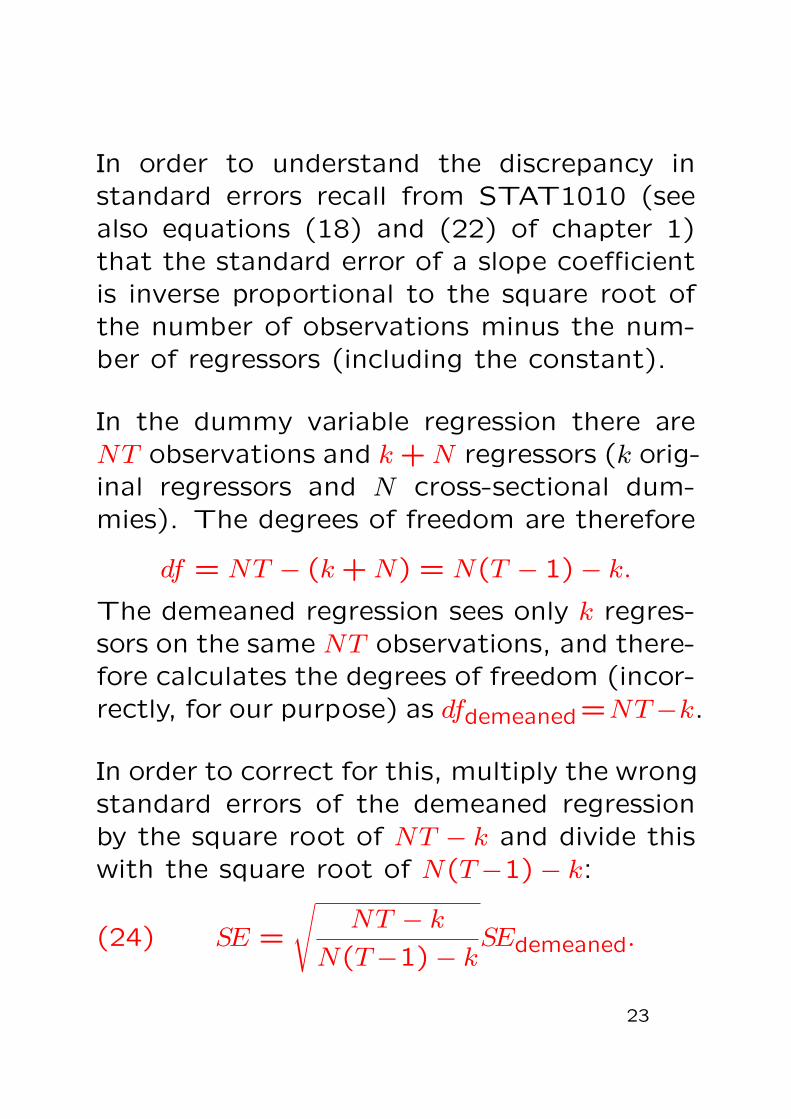
In order to understand the discrepancy instandard errors recall from STAT1010 (seealso equations (18) and (22) of chapter 1)that the standard error of a slope coefficientis inverse proportional to the square root ofthe number of observations minus the num-ber of regressors (including the constant).

In the dummy variable regression there areNT observations and k +N regressors (k orig-inal regressors and N cross-sectional dum-mies). The degrees of freedom are therefore

df = NT − (k +N) = N(T − 1)− k.The demeaned regression sees only k regres-sors on the same NT observations, and there-fore calculates the degrees of freedom (incor-rectly, for our purpose) as dfdemeaned =NT−k.

In order to correct for this, multiply the wrongstandard errors of the demeaned regressionby the square root of NT − k and divide thiswith the square root of N(T−1)− k:

(24) SE =

√NT − k

N(T−1)− kSEdemeaned.

23

Example 6. (continued)

We have N = 22 cross-sectional units andT = 9 time periods for a total of NT = 198observations. There is one dummy for theenterprize zone and eight year dummies fora total of k = 9 regressors. The correctionfactor for the standard errors is therefore√

NT − kN(T−1)− k

=

√22 · 9− 9

22 · 8− 9=

√189

167≈ 1.063831.

For example, multiplying the demeaned stan-

dard error of 0.052094 for the enterprise zone

dummy with the correction factor yields

1.063831 · 0.052094 = 0.055419,

which is the correct standard error that we

found from the dummy regression earlier.

Taken together with its coefficient estimate

of -0.1044 it will hence correctly reproduce

the t-statistic of -1.884 with p-value 0.0613,

however without the need to define 22 dummy

variables!

24

EViews can do the degrees of freedom ad-

justment automatically, if you tell it that you

have got panel data. In order to do that,

choose

Structure/Resize Current Page. . .

from the Proc Menue. In the Workfile Struc-

ture Window, choose ’Dated Panel’ and pro-

vide two identifyers: one for the cross section

and one for time.

This will provide you with a ’Panel Options’

tab in the estimation window. In order to ap-

ply the fixed effects estimator, (which, as we

discussed, is equivalent to a dummy variable

regression), change the effects specification

for the cross-section into ’Fixed’.

Note that EViews reports a constant C, even

though the demeaned regression shouldn’t

have any. C is to be interpreted as the aver-

age unobservable effect ai, or cross-sectional

average intercept.

25

Example 6. (continued)

Applying the Fixed Effects option in Eviews

yields

Dependent Variable: LUCLMSMethod: Panel Least SquaresDate: 12/05/12 Time: 11:47Sample: 1980 1988Periods included: 9Cross-sections included: 22Total panel (balanced) observations: 198


C 11.69439 0.042750 273.5544 0.0000D81 -0.321632 0.060457 -5.319980 0.0000D82 0.135496 0.060457 2.241179 0.0263D83 -0.219255 0.060457 -3.626613 0.0004D84 -0.579152 0.062318 -9.293490 0.0000D85 -0.591787 0.065495 -9.035540 0.0000D86 -0.621265 0.065495 -9.485616 0.0000D87 -0.888949 0.065495 -13.57268 0.0000D88 -1.227633 0.065495 -18.74379 0.0000EZ -0.104415 0.055419 -1.884091 0.0613

Effects Specification

Cross-section fixed (dummy variables)

R-squared 0.933188 Mean dependent var 11.19078Adjusted R-squared 0.921185 S.D. dependent var 0.714236S.E. of regression 0.200514 Akaike info criterion -0.233004Sum squared resid 6.714401 Schwarz criterion 0.281826Log likelihood 54.06741 Hannan-Quinn criter. -0.024618F-statistic 77.75116 Durbin-Watson stat 1.306450Prob(F-statistic) 0.000000

The output coincides with that obtained from

the dummy variable regression. C is the av-

erage of the cross-sectional city dummies C1

to C22.

26

R2 in Fixed Effects Estimation

Note from the preceding example that while

both the dummy regression and the fixed ef-

fects estimation yield an identical coefficient

of determination of R2 = 0.933188, it dif-

fers from R2 = 0.841596, which we obtained

when calculating the FE estimator by hand.

Both ways of calculating R2 are used.

The lower R2 obtained from estimating (23)

has the more intuitive interpretation as the

amount of variation in yit explained by the

time variation in the explanatory variables.

The higher R2 obtained in fixed effects esti-

mation and dummy variable regressions should

be used in F-tests when for example test-

ing for joint significance of the unobservables

ai, that is the cross-sectional dummies in

dummy variable regression.

27

Limitations

As with first differencing, the fact that we

eliminated the unobservables ai in estimation

of (23) implies that any explanatory variable

that is constant over time gets swept away by

the fixed effects transformation. Therefore

we cannot include dummies such as gender

or race.

If we furthermore include a full set of time

dummies, then, in order to avoid exact mul-

ticollinearity, we may neither include variables

which change by a constant amount through

time, such as working experience. Their ef-

fect will be absorbed by the year dummies in

the same way as the effect of time-constant

cross-sectional dummies is absorbed by the

unobservables.

28

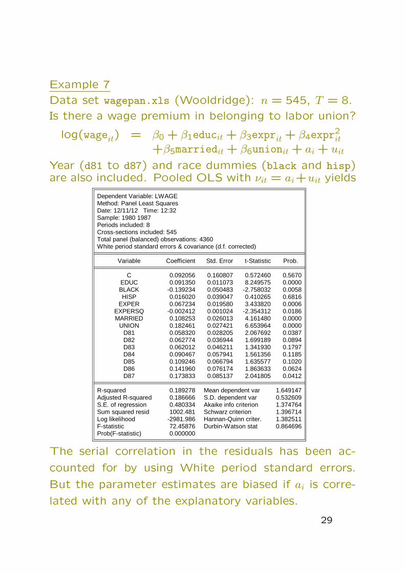
Example 7

Data set wagepan.xls (Wooldridge): n = 545, T = 8.

Is there a wage premium in belonging to labor union?

log(wageit) = β0 + β1educit + β3exprit + β4expr2it

+β5marriedit + β6unionit + ai + uit

Year (d81 to d87) and race dummies (black and hisp)are also included. Pooled OLS with νit = ai+uit yields

Dependent Variable: LWAGEMethod: Panel Least SquaresDate: 12/11/12 Time: 12:32Sample: 1980 1987Periods included: 8Cross-sections included: 545Total panel (balanced) observations: 4360White period standard errors & covariance (d.f. corrected)


C 0.092056 0.160807 0.572460 0.5670EDUC 0.091350 0.011073 8.249575 0.0000BLACK -0.139234 0.050483 -2.758032 0.0058HISP 0.016020 0.039047 0.410265 0.6816

EXPER 0.067234 0.019580 3.433820 0.0006EXPERSQ -0.002412 0.001024 -2.354312 0.0186MARRIED 0.108253 0.026013 4.161480 0.0000

UNION 0.182461 0.027421 6.653964 0.0000D81 0.058320 0.028205 2.067692 0.0387D82 0.062774 0.036944 1.699189 0.0894D83 0.062012 0.046211 1.341930 0.1797D84 0.090467 0.057941 1.561356 0.1185D85 0.109246 0.066794 1.635577 0.1020D86 0.141960 0.076174 1.863633 0.0624D87 0.173833 0.085137 2.041805 0.0412


The serial correlation in the residuals has been ac-

counted for by using White period standard errors.

But the parameter estimates are biased if ai is corre-

lated with any of the explanatory variables.

29

Example 7 (continued.)

Fixed Effects estimation yields

Dependent Variable: LWAGEMethod: Panel Least SquaresDate: 11/26/12 Time: 12:31Sample: 1980 1987Periods included: 8Cross-sections included: 545Total panel (balanced) observations: 4360


C 1.426019 0.018341 77.74835 0.0000EXPERSQ -0.005185 0.000704 -7.361196 0.0000MARRIED 0.046680 0.018310 2.549385 0.0108

UNION 0.080002 0.019310 4.142962 0.0000D81 0.151191 0.021949 6.888319 0.0000D82 0.252971 0.024418 10.35982 0.0000D83 0.354444 0.029242 12.12111 0.0000D84 0.490115 0.036227 13.52914 0.0000D85 0.617482 0.045244 13.64797 0.0000D86 0.765497 0.056128 13.63847 0.0000D87 0.925025 0.068773 13.45039 0.0000




Note that we could not include the years of education

and the race dummies, because they remain constant

through time for each cross section. Likewise we could

not include years of working experience, because they

change by the same amount for all cross sections, and

we included already a full set of year dummies.

The large changes in the premium estimates for mar-

riage and union membership suggests that ai is corre-

lated with some of the explanatory variables.

30

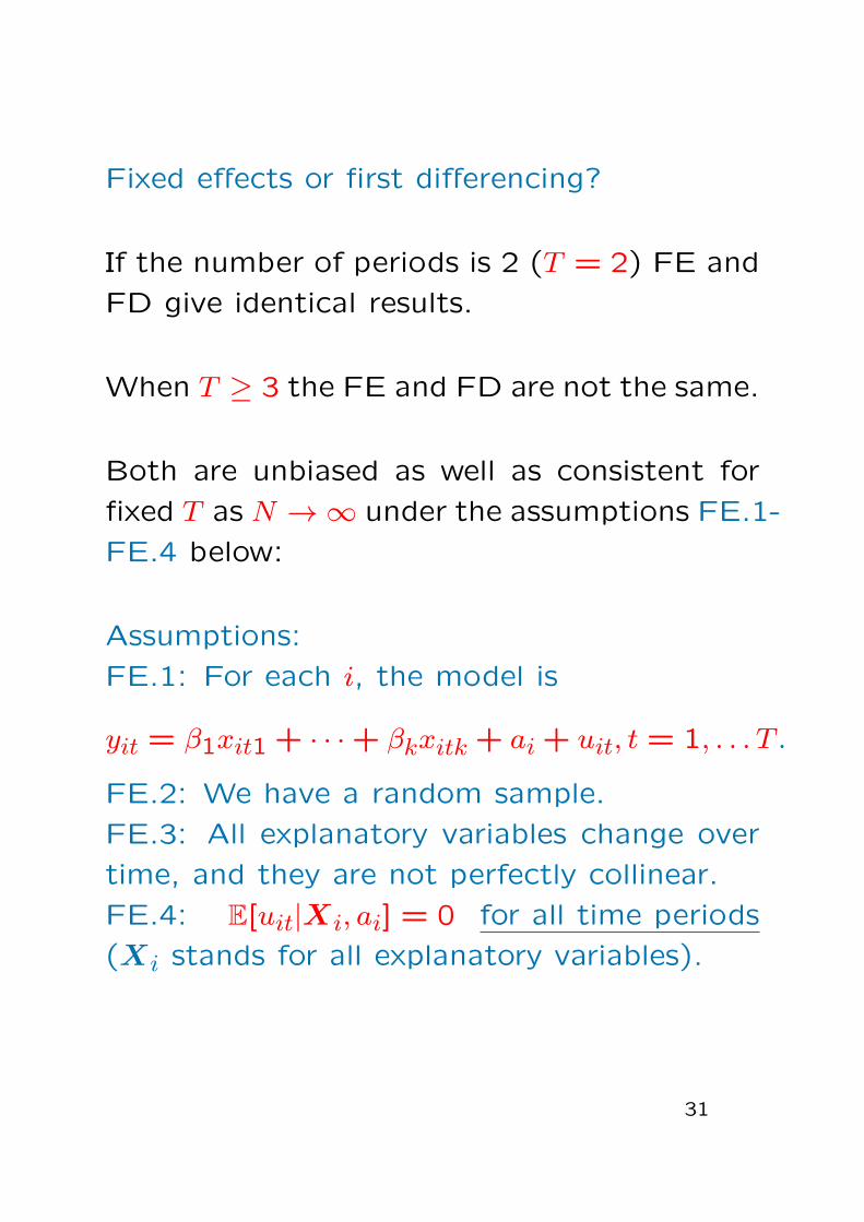
Fixed effects or first differencing?

If the number of periods is 2 (T = 2) FE and

FD give identical results.

When T ≥ 3 the FE and FD are not the same.

Both are unbiased as well as consistent for

fixed T as N →∞ under the assumptions FE.1-

FE.4 below:

Assumptions:

FE.1: For each i, the model is

yit = β1xit1 + · · ·+ βkxitk + ai + uit, t = 1, . . . T .

FE.2: We have a random sample.

FE.3: All explanatory variables change over

time, and they are not perfectly collinear.

FE.4: E[uit|Xi, ai] = 0 for all time periods

(Xi stands for all explanatory variables).

31

If we add the following two assumptions, FE

is the best linear unbiased estimator:

FE.5: Var[uit|Xi, ai] = σ2u for all t = 1, . . . , T .

FE.6: Cov[uit, uis|Xi, ai] = 0 for all t 6= s.

In that case FD is worse than FE because

FD is linear and unbiased under FE.1–FE.4.

While this looks like a clear case for FE, it is

not, because often FE.6 is violated. If uit is

(highly) serially correlated, ∆uit may be less

serially correlated, which may favor FD over

FE. However, typically T is rather small, such

that serial correlation is difficult to observe.

Usually it is best to check both FE and FD.

If we add as a last assumption

FE.7: uit|Xi, ai ∼ NID(0, σ2u),

then we may use exact t and F-statistics.

Otherwise they hold only asymptotically for

large N and T .

32

Balanced and unbalanced panels

A data set is called a balanced panel if thesame number of time series observations areavailable for each cross section units. Thatis T is the same for all individuals. The totalnumber of observations in a balanced panelis NT .

All the above examples are balanced paneldata sets.

If some cross section units have missing ob-servations, which implies that for an individ-ual i there are available Ti time period obser-vations i = 1, . . . , N , Ti 6= Tj for some i andj, we call the data set an unbalanced panel.The total number of observations in an un-balanced panel is T1 + · · ·+ TN .

In most cases unbalanced panels do not causemajor problems to fixed effect estimation.

Modern software packages make appropriateadjustments to estimation results.

33

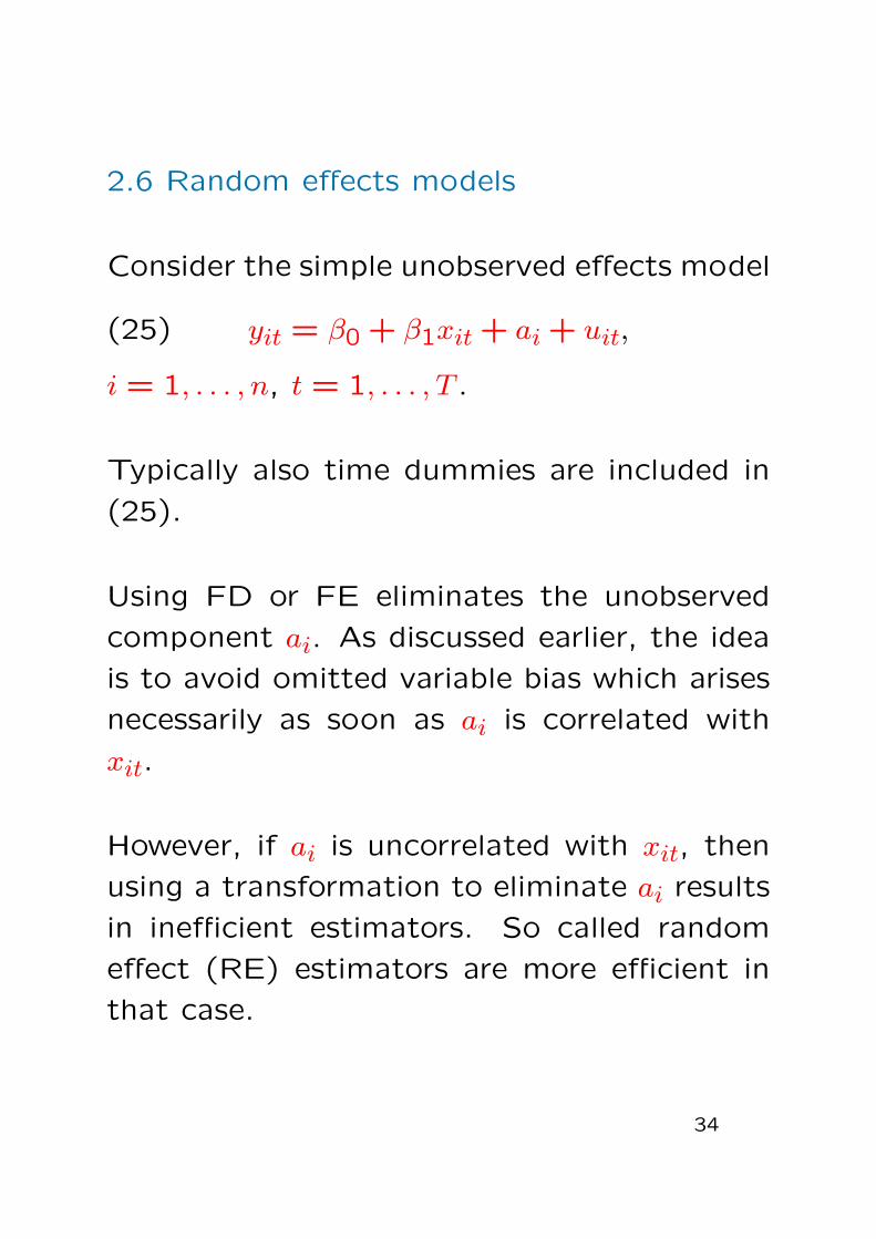
2.6 Random effects models

Consider the simple unobserved effects model

(25) yit = β0 + β1xit + ai + uit,

i = 1, . . . , n, t = 1, . . . , T .

Typically also time dummies are included in

(25).

Using FD or FE eliminates the unobserved

component ai. As discussed earlier, the idea

is to avoid omitted variable bias which arises

necessarily as soon as ai is correlated with

xit.

However, if ai is uncorrelated with xit, then

using a transformation to eliminate ai results

in inefficient estimators. So called random

effect (RE) estimators are more efficient in

that case.

34

Generally, we call the model in equation (25)

the random effects model if ai is uncorre-

lated with all explanatory variables, i.e.,

(26) Cov[xit, ai] = 0, t = 1, . . . , T .

How to estimate β1 efficiently?

If (26) holds, β1 can be estimated consis-

tently from a single cross section. So in prin-

ciple, there is no need for panel data at all.

But using a single cross section obviously dis-

cards a lot lot of useful information.

35

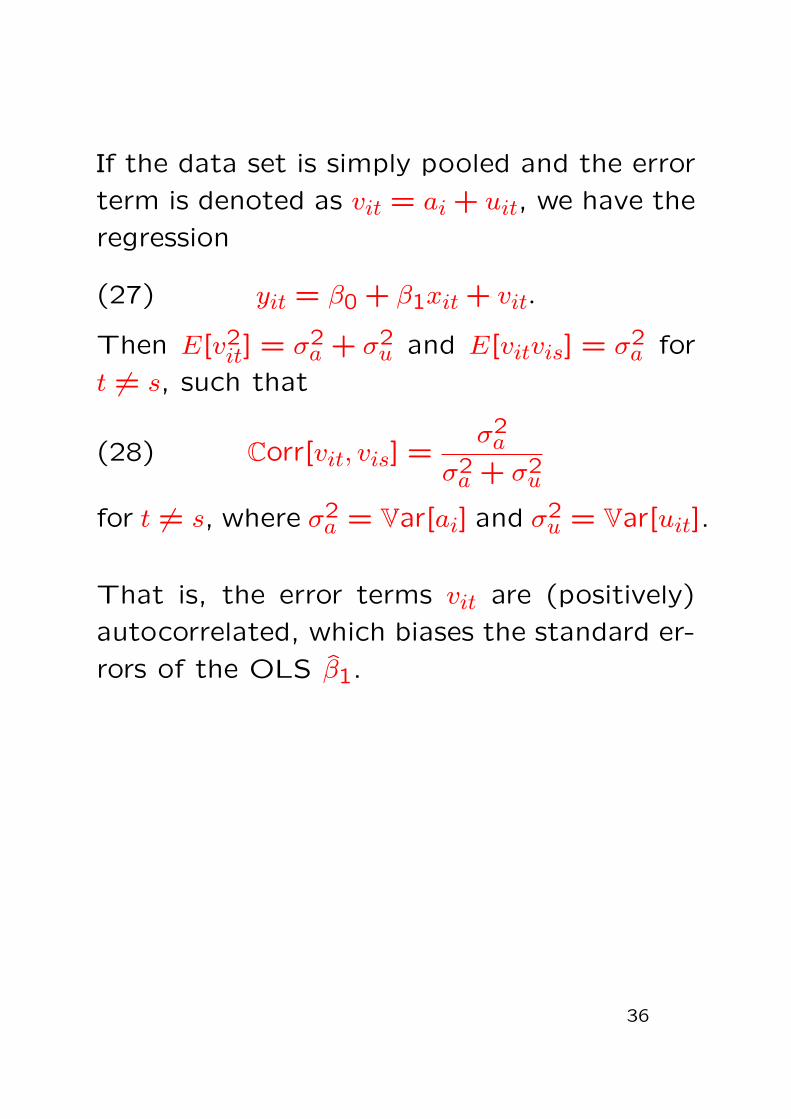
If the data set is simply pooled and the error

term is denoted as vit = ai + uit, we have the

regression

(27) yit = β0 + β1xit + vit.

Then E[v2it] = σ2

a + σ2u and E[vitvis] = σ2

a for

t 6= s, such that

(28) Corr[vit, vis] =σ2a

σ2a + σ2

u

for t 6= s, where σ2a = Var[ai] and σ2

u = Var[uit].

That is, the error terms vit are (positively)

autocorrelated, which biases the standard er-

rors of the OLS β1.

36

If σ2a and σ2

u were known, optimal estimators(BLUE) would be obtained by generalizedleast squares (GLS), which in this case wouldreduce to estimating the regression slope co-efficients from the quasi demeaned equation(29)yit−λyt = β0(1−λ) + β1(xit−λxi) + (vit−λvi),

where

(30) λ = 1−(

σ2u

σ2u + Tσ2

a

)12

.

In practice σ2u and σ2

a are unknown, but theycan be estimated for example as follows:

Estimate (27) from the pooled data set anduse the OLS residuals vit to estimate σ2

a fromthe average covariance of vit and vis for t 6= s.

In the second step, estimate σ2u from the vari-

ance of the OLS residuals vit as σ2u = σ2

ν − σ2a .

Finally plug these estimates of σ2a and σ2

u intoequation (30). Regression packages do thisautomatically.

37

The resulting GLS estimators for the regres-

sion slope coefficients are called random

effects estimators (RE estimators). Other

estimators of σ2a and σ2

u (and therefore λ)

are available. The particular version we dis-

cussed is the Swamy-Arora estimator.

Under the random effects assumptions∗ the

estimators are consistent, but not unbiased.

They are also asymptotically normal as N →∞for fixed T .

However, for small N and large T the proper-

ties of the RE estimator are largely unknown.

∗The ideal random effects assumptions include FE.1,FE.2, FE.4–FE.6.

FE.3 is replaced withRE.3: There are no perfect linear relationshipsamong the explanatory variables.RE.4: In addition of FE.4, E[ai|Xi] = 0.

38

Note that λ = 0 in (29) corresponds to pooled

regression and λ = 1 to FE, such that for

σ2u � σ2

a (λ ≈ 1) RE estimates will be sim-

iliar to FE estimates, whereas for σ2u � σ2

a

(λ ≈ 0) RE estimates will resemble pooled

OLS estimates.


Note that the constant dummies black and

hisp and the variable with constant change

exper, which dropped out with the FE method,

can be estimated with RE.

λ = 1−(

0.3512

0.3512 + 8 · 0.32462

)1/2

= 0.643,

such that the RE estimates lie closer to the

FE estimates than to the pooled OLS esti-

mates.

Applying RE is probably not appropriate in

this case, because, as discussed earlier, the

unobservable ai is probably correlated with

some of the explanatory variables.

39

EViews output for RE estimation:

Dependent Variable: LWAGEMethod: Panel EGLS (Cross-section random effects)Date: 11/26/12 Time: 12:26Sample: 1980 1987Periods included: 8Cross-sections included: 545Total panel (balanced) observations: 4360Swamy and Arora estimator of component variances


C 0.023586 0.150265 0.156965 0.8753EDUC 0.091876 0.010631 8.642166 0.0000BLACK -0.139377 0.047595 -2.928388 0.0034HISP 0.021732 0.042492 0.511429 0.6091

EXPER 0.105755 0.015326 6.900482 0.0000EXPERSQ -0.004724 0.000688 -6.869682 0.0000MARRIED 0.063986 0.016729 3.824781 0.0001

UNION 0.106134 0.017806 5.960582 0.0000D81 0.040462 0.024628 1.642894 0.1005D82 0.030921 0.032255 0.958646 0.3378D83 0.020281 0.041471 0.489036 0.6248D84 0.043119 0.051179 0.842509 0.3995D85 0.057815 0.061068 0.946733 0.3438D86 0.091948 0.071039 1.294334 0.1956D87 0.134929 0.081096 1.663821 0.0962

Effects SpecificationS.D. Rho

Cross-section random 0.324603 0.4610Idiosyncratic random 0.350990 0.5390

Weighted Statistics

R-squared 0.180618 Mean dependent var 0.588893Adjusted R-squared 0.177977 S.D. dependent var 0.388166S.E. of regression 0.351932 Sum squared resid 538.1558F-statistic 68.41243 Durbin-Watson stat 1.589754Prob(F-statistic) 0.000000

Unweighted Statistics

R-squared 0.182847 Mean dependent var 1.649147Sum squared resid 1010.433 Durbin-Watson stat 0.846702

40

Random effects or fixed effects?

FE is widely considered preferable because it

allows correlation between ai and x variables.

Given that the common effects, aggregated

to ai is not correlated with x variables, an

obvious advantage of the RE is that it allows

also estimation of the effects of factors that

do not change in time (like education in the

above example).

Typically the condition that common effects

ai is not correlated with the regressors (x-

variables) should be considered more like an

exception than a rule, which favors FE.

Whether this condition is met, can be tested

with the Hausman test to be discussed in the

following.

41

Hausman specification test

Hausman (1978) devised a test for the or-thogonality of the common effects (ai) andthe regressors.

The basic idea of the test relies on the factthat under the null hypothesis of orthogonal-ity both OLS and GLS are consistent, whileunder the alternative hypothesis GLS is notconsistent. Thus, under the null hypothe-sis OLS and GLS estimates should not differmuch from each other.

The Hausman test statistic is a transforma-tion of the differences between the parame-ter estimates obtained from RE and FE es-timation, which becomes asymptotically χ2-distributed under the null hypothesis (26)

H0 : Cov[xit, ai] = 0, t = 1, . . . , T.

The degrees of freedom are the number of re-gressors, where only those regressors may beincluded which are estimable with FE, thatis, time-constant variables must be dropped(also constant time changes, if year dummiesare included).

42

In order to perform the Hausman test in EViews,

first estimate the model with RE including

only those regressors, which are estimable

with FE as well. Then select

View/ Fixed/Random Effects Testing/

Correlated Random Effects - Hausman Test.

The first part of the output is the Hausman

test statistic with degrees of freedom and p-

value. The second part lists the parameter

estimates for both FE and RE estimation.

The final third part is more detailed FE esti-

mation output.


As expected, the Hausman test strongly re-

jects the null hypothesis, that ai would be

uncorrelated with all explanatory variables.

Therefore, RE is inappropriate and we must

use FE parameter estimates instead.

43

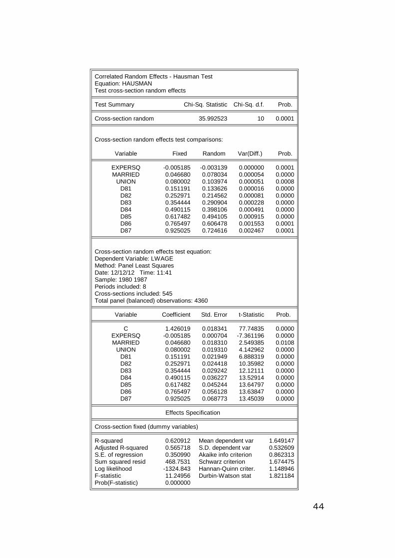
Correlated Random Effects - Hausman TestEquation: HAUSMANTest cross-section random effects

Test Summary Chi-Sq. Statistic Chi-Sq. d.f. Prob.

Cross-section random 35.992523 10 0.0001

Cross-section random effects test comparisons:

Variable Fixed Random Var(Diff.) Prob.

EXPERSQ -0.005185 -0.003139 0.000000 0.0001MARRIED 0.046680 0.078034 0.000054 0.0000

UNION 0.080002 0.103974 0.000051 0.0008D81 0.151191 0.133626 0.000016 0.0000D82 0.252971 0.214562 0.000081 0.0000D83 0.354444 0.290904 0.000228 0.0000D84 0.490115 0.398106 0.000491 0.0000D85 0.617482 0.494105 0.000915 0.0000D86 0.765497 0.606478 0.001553 0.0001D87 0.925025 0.724616 0.002467 0.0001

Cross-section random effects test equation:Dependent Variable: LWAGEMethod: Panel Least SquaresDate: 12/12/12 Time: 11:41Sample: 1980 1987Periods included: 8Cross-sections included: 545Total panel (balanced) observations: 4360


C 1.426019 0.018341 77.74835 0.0000EXPERSQ -0.005185 0.000704 -7.361196 0.0000MARRIED 0.046680 0.018310 2.549385 0.0108

UNION 0.080002 0.019310 4.142962 0.0000D81 0.151191 0.021949 6.888319 0.0000D82 0.252971 0.024418 10.35982 0.0000D83 0.354444 0.029242 12.12111 0.0000D84 0.490115 0.036227 13.52914 0.0000D85 0.617482 0.045244 13.64797 0.0000D86 0.765497 0.056128 13.63847 0.0000D87 0.925025 0.068773 13.45039 0.0000




44

Documents

2. Pooled Cross Sections and Panels Pooled Cross Sections ...lipas.uwasa.fi/~bepa/Panels.pdf · Pooled Cross Sections and Panels 2.1 Pooled Cross Sections versus Panel Data Pooled