2. One-Dimensional Systolic Arrays for Multidimensional Convolution and ResampHng

H.T. Kung 1 and R.L. Picard

We present one-dimensional systolic arrays for performing two- or higher­dimensional convolution and resampling. These one-dimensional arrays are characterized by the fact that their I/O bandwidth requirement is indepen­dent of the size of the convolution kernel. This contrasts with alternate two-dimensional array solutions, for which the I/O bandwidth must increase as the kernel size increases. The proposed architecture is ideal for VLSI implementation-an arbitrarily large kernel can be handled by simply extend­ing the linear systolic array with simple processors of the same type, so that one processor corresponds to each kernel element.

2.1 Background

Multidimensional convolution and the related resampling computation consti­tute some of the most compute-intensive tasks in image processing. For example, a two-dimensional (2-D) convolution with a general 4 x 4 kernel would require 16 multiplications and 15 additions to be performed for gen­erating each output pixel. To perform this convolution on a 1000 x 1000 image at the video rate would require the computing power of over 100 VAX-11/780s. If the kernel is larger or the dimensionality higher, even more computation power would be required. Though computationally demanding, multidimensional convolution and resampling are highly regular computations. We will show how to exploit this regularity and build cost-effective, high-throughput pipelined systems to perform 2-D and higher-dimensional convolution and re­sampling.

These pipelined designs are based on the systolic array architecture [2.1,2]. A systolic array organizes a regular computation such as the 2-D convolution through a lattice of identical function modules called cells. Unlike other parallel processors employing a lattice of function modules,

1 H.T. Kung was supported in part by the Office of Naval Research under Con­tracts N00014-76-C-0370, NR 044-422 and N00014-80-C-0236, NR 048-659

9

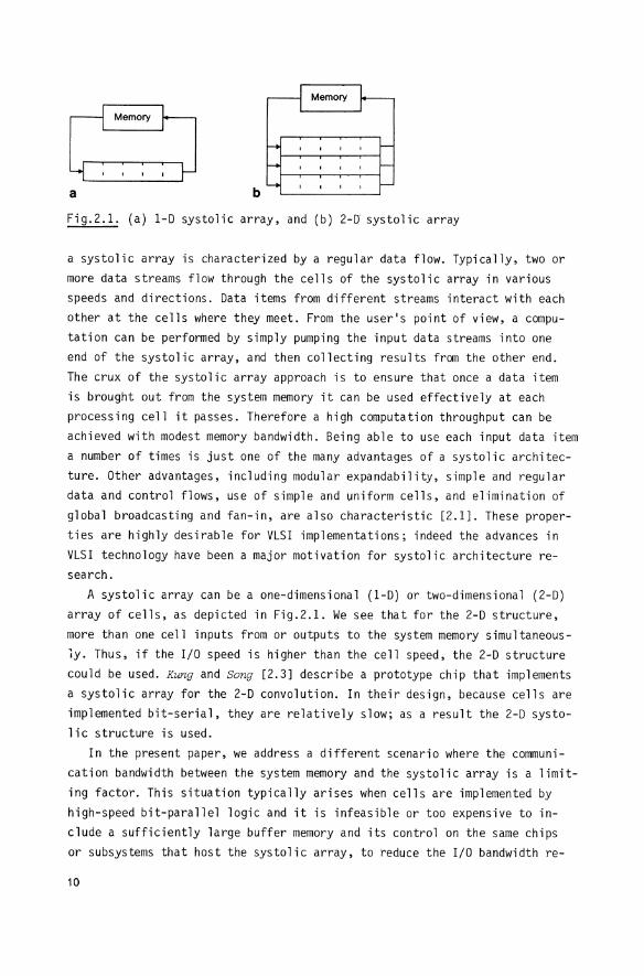
a b

Fig.2.1. (a) 1-0 systolic array, and (b) 2-D' systolic array

a systolic array is characterized by a regular data flow. Typically, two or more data streams flow through the cells of the systolic array in various speeds and directions. Data items from different streams interact with each other at the cells where they meet. From the user's point of view, a compu­tation can be performed by simply pumping the input data streams into one end of the systolic array, and then collecting results from the other end. The crux of the systolic array approach is to ensure that once a data item is brought out from the system memory it can be used effectively at each processing cell it passes. Therefore a high computation throughput can be achieved with modest memory bandwidth. Being able to use each input data item a number of times is just one of the many advantages of a systolic architec­ture. Other advantages, including modular expandability, simple and regular data and control flows, use of simple and uniform cells, and elimination of global broadcasting and fan-in, are also characteristic [2.1]. These proper­ties are highly desirable for VLSI implementations; indeed the advances in VLSI technology have been a major motivation for systolic architecture re­search.

A systolic array can be a one-dimensional (1-0) or two-dimensional (2-D) array of cells, as depicted in Fig.2.1. We see that for the 2-D structure, more than one cell inputs from or outputs to the system memory simultaneous­ly. Thus, if the I/O speed is higher than the cell speed, the 2-D structure could be used. Kung and Song [2.3] describe a prototype chip that implements a systolic array for the 2-D convolution. In their design, because cells are implemented bit-serial, they are relatively slow; as a result the 2-D systo­lic structure is used.

In the present paper, we address a different scenario where the communi­cation bandwidth between the system memory and the systolic array is a limit­ing factor. This situation typically arises when cells are implemented by high-speed bit-parallel logic and it is infeasible or too expensive to in­clude a sufficiently large buffer memory and its control on the same chips or subsystems that host the systolic array, to reduce the I/O bandwidth re-

10

quirement. In this case the bandwidth of memory, bus or pin, rather than the speed of the cells, is the bottleneck for achieving high system throughput. Therefore, it is appropriate to use the 1-0 systolic structure, that has the minimum possible I/O bandwidth requirement. In Sect.2.2, we present the fun­damental result of this paper-fully utilized 1-0 systolic arrays for per­forming 2-0 and higher-dimensional convolutions. Extensions of this result to other related problems, such as resampling, are given in Sects.2.3,4, where the requirements imposed on systolic array implementations by various classes of convolutions are also discussed. In Sect.2.S are concluding re­marks and a list of problems that have systolic solutions.

2.2 Systolic Convolution Arrays

We first review a 1-0 systolic array for the 1-0 convolution, and then show how this basic design can be extended to a 1-0 systolic array for 2-0, 3-0 and higher-dimensional convolutions.

2.2. 7 Systolic Array for 7-0 Convolution

The 1-0 convolution problem is defined as follows:

Given the kernel as a sequence of weights (w1,w2, ... ,wk) and the input se­quence (xl'x2, ... ,xn), eompute the output sequence (Yl'Y2'··· 'Yn+l-k)' defined by Yi =w1xi +w2xi+l + ... + wkxi+k_1·

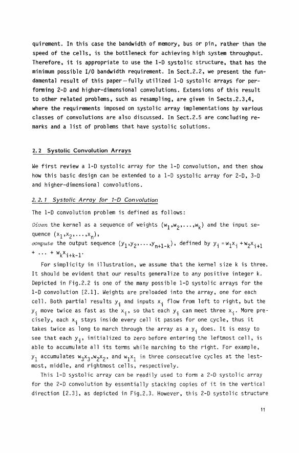
For simplicity in illustration, we assume that the kernel size k is three. It should be evident that our results generalize to any positive integer k. Oepicted in Fig.2.2 is one of the many possible 1-0 systolic arrays for the 1-0 convolution [2.1]. Weights are preloaded into the array, one for each cell. Both partial results Yi and inputs Xi flow from left to right, but the Yi move twice as fast as the Xi' so that each Yi can meet three Xi. More pre­cisely, each Xi stays inside every cell it passes for one cycle, thus it takes twice as long to march through the array as a Yi does. It is easy to see that each Yi' initialized to zero before entering the leftmost cell, is able to accumulate all its terms while marching to the right. For example, Yl accumulates w3x3,w2x2, and w1x1 in three consecutive cycles at the lest­most, middle, and rightmost cells, respectively.

This 1-0 systolic array can be readily used to form a 2-0 systolic array for the 2-0 convolution by essentially stacking copies of it in the vertical direction [2.3], as depicted in Fig.2.3. However, this 2-0 systolic structure

11

a

b Y oul .. Yin + Win' Xin

X .. Xin

Xoul .. X

Fig.2.2, (a) Systolic array for 1-D convolution using a kernel of size 3, and (b) the cell definition

x

x

x

y

Fig.2.3. 2-D systolic array obtained by stacking 1-D arrays

has high I/O bandwidth requirements when the kernel size k is large, and thus is inappropriate for the scenario addressed in this paper. The task we

face is to design a new 1-D systolic array that is capable of performing the 2-D convolution with full utilization of all its cells. The next section

shows how this can be accomplished.

2.2.2 7-0 Systolic Array for 2-D Convolution

The 2-D convolution problem is defined as follows:

Given the weights w .. for i,j =1,2, ... ,k that form a kxk kernel, and the lJ

input image Xu for i,j = 1,2, ... ,n, compute the output image y .. for i,j =1,2, ... , n defined by

lJ

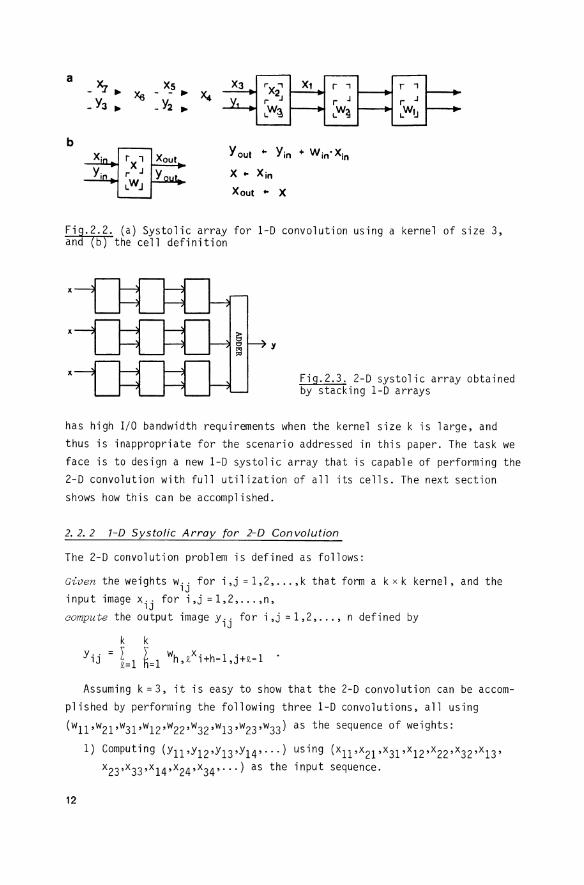
Assuming k = 3, it is easy to show that the 2-D convolution can be accom­plished by performing the following three 1-D convolutions, all using

(w11,w21,w31,w12,w22,w32,w13,w23,w33) as the sequence of weights:

12

1) Computing (Y11'Y12'Y13'Y14"") using (x11,x21,x31,x12,x22,x32,x13' x23,x33,x14,x24,x34" .. ) as the input sequence.

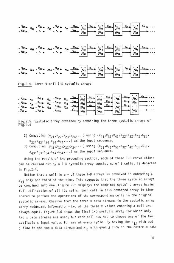
Fig.2.4. Three 9-cell 1-0 systolic arrays

- ~. ~ _ XIS. 'U4 - X24. x,. - ~. ~ -x... 'U4 - X24. X!3 _ >!Is. Xs4-~. %4 - XSl. ~ _ Y12. _ Y3I • - Y21.

Fig.2.5. Systolic array obtained by combining the three systolic arrays of Fig.2.4

2) Computing (Y21'Y22'Y23'Y24"") using (x21,x31,x41,x22,x32,x42,x23' x33,x43,x24,x34,x44"") as the input sequence.

3) Computing (Y31'Y32'Y33'Y34"") using (x31,x41,x51,x32,x42,x52,x33' x43,x53,x34,x44,x54"") as the input sequence.

Using the result of the preceding section, each of these 1-0 convolutions can be carried out by a 1-0 systolic array consisting of 9 cells, as depicted in Fig.2.4.

Notice that a cell in any of these 1-0 arrays is involved in computing a Yij only one third of the time. This suggests that the three systolic arrays be combined into one. Figure 2.5 displays the combined systolic array having full utilization of all its cells. Each cell in this combined array is time­shared to perform the operations of the corresponding cells in the original systolic arrays. Observe that the three x data streams in the systolic array carry redundant information-two of the three x values entering a cell are always equal. Figure 2.6 shows the final 1-0 systolic array for which only two x data streams are used, but each cell now has to choose one of the two available x input values for use at every cycle. By having the x .. with odd

lJ j flow in the top x data stream and x.· with even j flow in the bottom x data

lJ

13

a _ ~5~

~ _ XIS ~ • _ XS3~

~ - '!.. ~ Xs4-x.w~ ~4

_ X~~ X14

_ Y12 ~ _ Y3I ~ _ Y2l ~

b Xoul .. X; X" Xin

XOU! .. ~; x .. )(in

You! .. Yin + W 'Xin OR Yin ... W oXin

Fig.2.6. (a) 1-0 systolic array for 2-D convolutions and (b) the cell defi­mtion

MEMORY

1-D SYSTOLIC ARRAY Fig.2.7. Use of cache to eliminate reaccess of input pixels

stream, as shown in the figure, the choice of the x input at each cell is easily determined. The simple rule is that a cell should use an x data stream for three consecutive cycles before switching to the other stream, and con­tinue alternating in this manner.

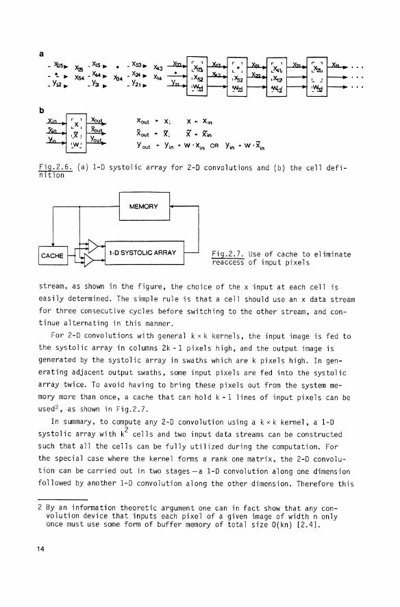
For 2-D convolutions with general k x k kernels, the input image is fed to the systol ic array in columns 2k -1 pixel s high, and the output image is generated by the systolic array in swaths which are k pixels high. In gen­erating adjacent output swaths, some input pixels are fed into the systolic array twice. To avoid having to bring these pixels out from the system me­mory more than once, a cache that can hold k -1 lines of input pixels can be used 2 , as shown in Fig.2.7.

In summary, to compute any 2-D convolution using a k x k kernel, a 1-0 systolic array with k2 cells and two input data streams can be constructed such that all the cells can be fully utilized during the computation. For the special case where the kernel forms a rank one matrix, the 2-D convolu­tion can be carried out in two stages-a 1-0 convolution along one dimension followed by another 1-0 convolution along the other dimension. Therefore this

2 By an information theoretic argument one can in fact show that any con­volution device that inputs each pixel of a given image of width n only once must use some form of buffer memory of total size O(kn) [2.4].

14

degenerate case requires only 1-0 systolic arrays with k cells for each of the 1-0 convolutions.

2.2.3 1-D Systolic Array for Multidimensional Convolution

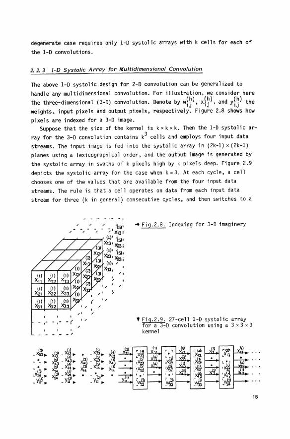
The above 1-0 systolic design for 2-D convolution can be generalized to handle any multidimensional convolution. the three-dimensional (3-D) convolution. weights, input pixels and output pixels,

For illustration, we consider here (h) (h) (h) Denote by wij , xij , and Yij the

respectively. Figure 2.8 shows how pixels are indexed for a 3-~ image.

Suppose that the size of the kernel is k x k x k. Then the 1-0 systolic ar­ray for the 3-~ convolution contains k3 cells and employs four input data streams. The input image is fed into the systolic array in (2k-1) x (2k-1) planes using a lexicographical order, and the output image is generated by the systolic array in swaths of k pixels high by k pixels deep. Figure 2.9 depicts the systolic array for the case when k=3. At each cycle, a cell chooses one of the values that are available from the four input data streams. The rule is that a cell operates on data from each input data stream for three (k in general) consecutive cycles, and then switches to a

- - .- -. - - I

,,! /

- .- -.- - ( I /

I

- - - - -"

(~ ~ X(1J x(s) _ X53. - 12· _ .3:3.

• >&J _ x!.,.'j - - . -X4J • 3.

• tJ _X~4. ti ('j - - . J~ X{1J JG4 XJ4 •

x{J) • •

:~: X24 - ~. - \2). _ Yu • _ Yu •

• Fig.2.8. Indexing for 3-D imaginery

• Fig.2.9. 27-cell 1-0 systolic array for a 3-~ convolution using a 3 x 3 x 3 kennel

r (~ r , r (~ r(2)o

.~ • .X14 .X14 '-til !..4 '11 .;om , • I

,_X5:! I_~ ~>4lb ~~ I • I I • I ~xi'~ '~ ,- <2l

~ ~WJ ~

15

new stream. The order of choosing data streams is as follows: first, second, first; third, fourth, third; first, second, first; and so on. Therefore the switch between one pair of streams (the first and second) and the other (the third and fourth) occurs every nine (k2 in general) cycles.

The above approach extends systematically to any number of dimensions. For example, for the four-dimensional convolution, the switch between one set of four input streams and the other occurs every k3 cycles. This struc­tured approach to multidimensional convolution can make an unwieldy problem solvable by providing an optimized hardware configuration, as well as opti­mized data access and control mechanisms.

2.3 Variants in the Convolution Problem

Signal-processing and image-processing applications make extensive use of 2-D convolution-like calculations for filtering, enhancement, interpolation, and other similar functions. Thus the 1-0 systolic array for the 2-D convo­lution presented in the last section can potentially be used to implement any of these functions. Based on the dynamics of the convolutional kernels, these functions may be organized into three broad categories consisting of fixed, adaptive, and selectable kernels.

A fixed kernel convolution has only a single set of weights. Typically, this would be found in equipment custom-designed to perform one specific function, so the weights could be hard-wired into the machine. This could be the best alternative in detection or fixed-filtering applications where the primary objective is to minimize the recurring hardware cost.

The adaptive kernel class is a generalization of the fixed kernel class, the major difference being that the weights may be changed. This class di­vides further into two distinct subclasses. The first subclass is basically a fixed kernel, but where the weights may be initialized (down-loaded) with an arbitrary value whenever the convolver is quiescent. The second subclass, and one gaining a lot of attention in signal processing areas, is the "true" adaptive kernel. For this subclass, the weights may be altered by some ex­ternal source without interrupting the on-going convolution process. In this case, theweigths would be updated to reflect a change in the convolver's environment, often based on the convolver's own input or result stream. The critical parameter for this type of kernel is the adaptation time constant, that is, the rate at which the weights may be modified. This adaptation rate can easily be more than an order of magnitude slower than the data rate, being limited almost entirely by the complexity of the weight calculation.

16

Typically, calculating adaptive weights requires time-consuming inversion of a time-varying covariance matrix [2.5], although other systolic arrays could be used to speed up this calculation [2.6]. Also important is the guarantee that no erroneous results are produced during the transition from one weight set to another.

The final classification is selectable kerne}s, distinguished from the adaptive kernels by allowing only a limited chOice for the weights. Usually, the selectable kernels would be prestored in tables, instead of directly calculated, and the particular weights to be used are chosen by the value of a control variable associated with each desired output. Note that this permits the weights to change at the same rate as the data. This is a very important class of convolutions, including most forms of interpolation and resampling. This is also fundamental to the geometric correction or spatial warping of images.

In the next section, we discuss how the basic systolic design for the 2-D convolution, presented in Sect.2.2 can be reduced to practice for some of the applications mentioned above.

2.4 Implementation

Systolic processors are attractive candidates for custom-VLSI implementation, due mainly to their low I/O requirement, regular structure and localized in­terconnection. Despite this, much recent effort has been spent trying to adapt the systolic approach to use off-the-shelf integrated circuits as well [2.7,8]. This effort has two primary objectives: first, to provide a vehicle for evaluating the many and varied systolic architectural and algo­rithmic alternatives; and second, to demonstrate that the benefits of a sys­tolic processor are achievable even without going to custom integrated cir­cuits. This section will address issues related to custom VLSI implementa­tion as well as implementation by off-the-shelf, discrete components.

2. 4. 7 Basic Systolic Cell Design

A generic systolic cell for convolution-like computations needs a multiply­add unit, and the staging registers on input and output to permit each cell to function independently of its neighbors. The addition of a systolic con­trol path and a cell memory makes this an excellent building block for a linear systolic array. To implement the two-stream, 1-D systolic array for the 2-D convolution, this basic cell must be modified to include the second

17

CON'~~----------------------------------------••

-R E

.ss- ~ ADORE

AL PART!

RESUL

ODD INPUT

EVEN INPUT

T

T

~ --1 CELL I MEMORY

R _E

G

~S SELECT ~

r--R E a 5 T

..!!. r--

R E a 5 T

..!!.

-R E S U

r-- L

Lf T_

R R ADD E E G

MPY O_ S

5 '--- T T ...!i R

r--R E a 5 T

~

-R E a 5 T

.B..

Fig.2.IO. Basic two-stream systolic cell block diagram

systolic input path and the two-to-one multiplexer for stream selection. The resulting cell is diagrammed in Fig.2.l0. Note that each input stream in­cludes two registers to guarantee that it moves at half the rate of the out­put stream, as required in Sect.2.2.2.

The practtcality of this design can be illustrated by examlnlng a real problem, such as 4 x4 cubic resampling. This is the inner loop for general­ized spatial image warping, and is characteristic of the selected kernel ap­plications described in Sect.2.3. The control variable, in this case, is the fractional position in the input image of each output pixel. Specifying this fractional position with 5-bit resolution in both the line and pixel direc­tions will provide better than 0.1 pixel accuracy in the resampled image. A two-stream cell to accomplish this resampling could be constructed with 8-bit input paths and l2-bit weights. The 32 x 32 interpixel grid requires 1024 different weights in each cell memory, and a lO-bit systolic address

18

path derived from the fractional pixel location. A 12-bit multiplier with a 24-bit partial-product adder will allow full precision to be maintained throughout the calculation.

As indicated in Sect.2.2. for higher-dimensional (more than 2-D) convo­lutions the only modification required to the basic two-stream cell is the addition of the requisite number of systolic input streams. along ~lith the correspondingly sized multiplexer to select the proper data at each cell.

2. II. 2 Implementation by Discrete Components

For a low-cost implementation of the basic systolic cell described above. the multiplier will be the limiting function on the cell speed. Using a TRW MPY-12HJ gives a worse-case cell computation rate of 110 nanoseconds. A standard Schottky-TTL. carry look-ahead adder and a high-speed lKx4 static memory (e.g .• Intel 2148) are compatible with this overall computation rate. This results in a cell having an arithmetic rate of greater than 18 Million Operations Per Second (MOPS). using only 24 integrated circuits and co~ting less than $250.

The complete 4x4 (16-cell). two-stream systolic interpolator would have an aggregate performance of 288 MOPS. or an output rate of 9 megapixels per second. Using a rather conservative printed circuit (PC) board density of 0.75 square inches per 16-pin IC. this entire processor would fit on two large PC boards. The total board area would be less than 500 square inches and the total material cost under $5000.

The systolic array cell just described can be used for all three convolu­tional classes outlined in Sect.2.3. except with true adaptive kernels. This class can be easily included by adding an extra data path to write to cell memory. thereby allowing the weights to be modified without using one of the operational data paths.

One important observation must be made with respect to adaptive kernels. At the transition from one weight set to another. the implication is that all the weights must change before the next computation cycle to guarantee that the weights used will be entirely from one set. For the systolic pro­cessor though. this is not the case. The contribution of each weight to the final convolution occurs in separate cells. one clock time apart. So. the weights may also be updated in this sequential manner. For a convolution using a k x k kernel. the required input bandwidth to the cell memory is no· greater than the data input bandwidth, even though all k2 weights must be replaced between computations. As a consequence of this, the adaptation rate is limited to once every k2 cycles.

19

2. 4. 3 Custom VLSI Implementation by the PSC

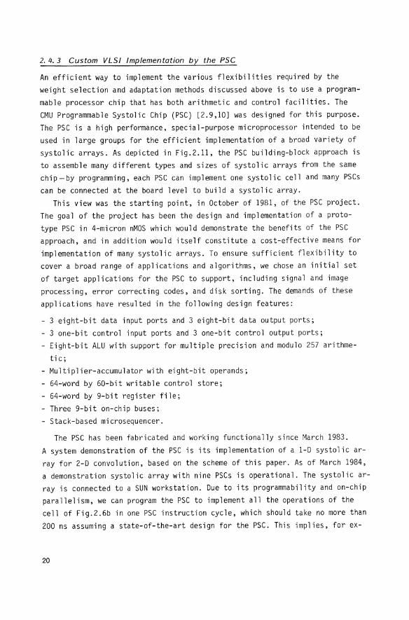
An efficient way to implement the various flexibilities required by the weight selection and adaptation methods discussed above is to use a program­mable processor chip that has both arithmetic and control facilities. The CMU Programmable Systolic Chip (PSC) [2.9,10] was designed for this purpose. The PSC is a high performance, special-purpose microprocessor intended to be used in large groups for the efficient implementation of a broad variety of systolic arrays. As depicted in Fig.2.11, the PSC building-block approach is to assemble many different types and sizes of systolic arrays from the same chip-by programming, each PSC can implement one systolic cell and many PSCs can be connected at the board level to build a systolic array.

This view was the starting point, in October of 1981, of the PSC project. The goal of the project has been the design and implementation of a proto­type PSC in 4-micron nMOS which would demonstrate the benefits of the PSC approach, and in addition would itself constitute a cost-effective means for implementation of many systolic arrays. To ensure sufficient flexibility to cover a broad range of applications and algorithms, we chose an initial set of target applications for the PSC to support, including signal and image processing, error correcting codes, and disk sorting. The demands of these applications have resulted in the following design features:

- 3 eight-bit data input ports and 3 eight-bit data output ports; - 3 one-bit control input ports and 3 one-bit control output ports; - Eight-bit ALU with support for multiple precision and modulo 257 arithme-

ti C;

- Multiplier-accumulator with eight-bit operands; - 54-word by 50-bit writable control store; - 64-word by 9-bit register file; - Three 9-bit on-chip buses;

Stack-based microsequencer.

The PSC has been fabricated and working functionally since March 1983.

A system demonstration of the PSC is its implementation of a 1-D systolic ar­ray for 2-D convolution, based on the scheme of this paper. As of March 1984, a demonstration systolic array with nine PSCs is operational. The systolic ar­ray is connected to a SUN workstation. Due to its programmability and on-chip parallelism, we can program the PSC to implement all the operations of the cell of Fig.2.6b in one PSC instruction cycle, which should take no more than 200 ns assuming a state-of-the-art design for the PSC. This implies, for ex-

20

aooo FiS.2.11. PSC: a building-block ChlP for a variety of systolic arrays

ample, that the 2-D convEllution with 5 x 5 kernels can be implemented by 25 linearly connected PSCs, capable of producing one output pixel every 200 ns.

For large kernels, it is necessary to save partial results Yi in double or higher precision to ensure numerical accuracy of the computed results. As for the case of systolic arrays for 1-0 convolution [2.1], this can be achieved most cost effectively by using a dual of the design in Fig.2.6, where partial results y. stay in cells but the x. and w .. move from cell to

1 1 lJ cell in the same direction but at two speeds. With this dual design, high-precision accumulation can be effectively achieved by the on-chip multiplier­accumulator circuit, and the number of bits to be transferred between cells is minimized. We of course still need to transfer the final computed values of the Yi out of the array, but they, being the final results, can be trun­cated and transferred in single precision. It is generally preferable to have the wij rather than the Xi going through an additional register in each cell, since there are two x data streams but only one weight stream. Sometimes the communication cost for the weight stream can be totally eli­minated if the register file of the PSC is large enough to hold a complete weight table.

2.5 Concluding Remarks

We have shown a regular and realizable systolic array architecture capable of performing multidimensional (n-O) convolutions with any kernel size kn. This array can fully utilize kn linearly connected cells, but more impor-

21

tantly, is sustained with a data input bandwidth which is independent of k n-l and requires less than 2 words per cell cycle. As a result, any convolu-

tion size (variation in k) can be handled with a fixed system input/output bandwidth capability, provided that kn cells are used. To accommodate a larger value of k only requires that the existing systolic array be extended linearly with the appropriate number of identical cells.

An important characteristic of the proposed systolic array is that the data all flow in one direction. This property implies that the systolic ar­ray can be made fault tolerant with little overheads, and can be transformed automatically into one where cells are implemented with pipelined functional units, using results of a recent paper [2.11]. For instance, the cells of floating-point systolic arrays are typically implemented with multipliers and adders with three or more pipeline stages. It is therefore important to make effective use of this second level of pipelining provided by the cells themselves to increase the throughput of the systolic array further. A dif­ferent two-level pipelined systolic array for multidimensional convolution was proposed previously [2.4], but that method requires a large buffer me­mory in every cell.

Multidimensional convolution and resampling represent just one class of computations suitable to systolic architectures. Recent research has shown that systolic architectures are possible for a wide class of compute-bound computations where multiple operations are performed on each data item in a repetitive and regular manner. This is especially true for much of the time­consuming "front-end processing" that deals with large amounts of data ob­tained directly from sensors in various signal- and image-processing appli­cation areas. To indicate the breadth of the systolic approach, the follow­ing is a partial list of problems for which systolic solutions exist.

a) Signal and Image Processing: FIR, IIR filtering 1-0, 2-D convolution and correlation 1-0, 2-D interpolation and resampling 1-0, 2-D median filtering discrete Fourier transforms geometric warping encoding/decoding for error correction

b) Matrix Arithmetic: - matrix-vector multiplication - matrix-matrix multiplication - matrix triangularization (soluHon of linear systems, matrix inversion)

22

- QR decomposition (least-squares computation, covariance matrix inversion) - singular value decomposition - eigenvalue computation - solution of triangular linear system - solution of toeplitz linear systems

c) Nonnumeric Applications: 1) data structures - stack, queue, priority queue - searching, dictionary - sorting 2) graph and geometric algorithms - transitive closure - minimum spanning trees - connected components

convex hulls 3) language recognizer

string matching - regular language recognition 4) dynamic programming 5) relational database operations 6) polynomial algorithms - polynomial multiplication and division

polynomial greatest common divisor 7) multiprecision integer arithmetic

integer multiplication and division integer greatest common divisor

8) Monte Carlo simulation.

Several theoretical frameworks for the design of systolic arrays are being developed [2.11-14]. Extensive references for the systolic literature can be found in separate papers [2.1,15]. Major efforts have now been started to build systolic processors and to use them for large, real-life applications. Practical issues on the implementation and use of systolic array processors in systems are beginning to receive substantial attention. Readers can follow some of the references of this paper for further infor­mation on systolic arrays and their implementation.

23

References

2.1 H.T. Kung: Why Systolic Architectures? Computer Mag. 15, 37-46 (January 1982)

2.2 H.T. Kung, C.E. Leiserson: Systolic Arrays (for VLSI), in Sparse Matrix Proceedings 1978, ed. by I.S. Duff and G.W. Stewart (Soc. for Industrial and Applied Mathematics, 1979) pp.256-282 A slightly different version appears in Introduction to VLSI Systems, ed. by C.A. Mead and L.A. Conway (Addison-Wesley, Reading, MA 1980) Sect.8.3

2.3 H.T. Kung, S.W. Song: A Systolic 2-D Convolution Chip, in Multicom­puters and Image Processing: Algorithms and Programs, ed. by K. Preston, Jr. and L. Uhr (Academic, New York 1982) pp.373-384

2.4 H.T. Kung, L.M. Ruane, D.W.L. Yen: Two-Level Pipelined Systolic Array for Multidimensional Convolution. Image and Vision Computing 1, 30-36 (1983) An improved version appears as a CMU Computer Science Department tech­nical report November 1982

2.5 R.A. Monzingo, T.W. Miller: Introduction to Adaptive Arrays (Wiley, New York 1980)

2.6 W.M. Gentleman, H.T. Kung: Matrix Triangularization by Systolic Arrays, in Real-Time Signal Processing IV, SPIE Symp. 298, 16-26 (Soc. Photo­Optical Instrumentation Engineers, 1981)

2.7 J.J. Symanski: NOSC Systolic Processor Testbed. Technical Report NOSC TO 588, Naval Ocean Systems Center (June 1983)

2.8 O.W.L. Yen, A.V. Kulkarni: Systolic Processing and an Implementation for Signal and Image Processing. IEEE Trans. C-31, 1000-1009 (1982)

2.9 A.L. Fisher, H.T. Kung, L.M. Monier, Y. Dohi: Architecture of the PSC: A Programmable Systolic Chip, in Proc. 10th Annual Intern. Symp. Com­puter Architecture (June 1983) pp.48-53

2.10 A.L. Fisher, H.T. Kung, L.M. Monier, H. Walker, Y. Dohi: Design of the PSC: A Programmable Systolic Chip, in Proc. 3rd Caltech Conf. on Very Large Scale Integration, ed. by R. Bryant (Computer Science Press, Rockville, MD 1983) pp.287-302

2.11 H.T. Kung, M. Lam: Fault-Tolerance and Two-Level Pipelining in VLSI Systolic Arrays, in Proc. Conf. Advanced Research in VLSI (Artech House, Inc., Cambridge, MA, January 1984) pp.74-83

2.12 H.T. Kung, W.T. Lin: An Algebra for VLSI Computation, in Elliptic Problem Solvers II, ed. by G. Birkhoff and A.L. Schoenstadt (Academic, New York 1983). Proc. Conf. on Elliptic Problem Solvers, January 1983

2.13 C.E. Leiserson, J.B. Saxe: Optimizing Synchronous Systems. J. VLSI and Computer Syst. 1, 41-68 (1983)

2.14 U. Weiser, A. Davis: A Wavefront Notation Tool for VLSI Array Design, in VLSI Systems and Computations, ed. by H.T. Kung, R.F. Sproull, and G.L. Steele, Jr. (Computer Science Press, Rockville, MD 1981) pr.226-234

2.15 A.L. Fisher, H.T. Kung: Special-Purpose VLSI Architectures: General Discussions and a Case Study, in VLSI and Modern Signal Processing (Prentice-Hall, Reading, MA 1982)

24