Embed Size (px)
Citation preview
High order �nite-di�erence approximations
of the wave equation with absorbing boundary conditions:
a stability analysis
Alain Sei �
Submitted to SIAM Journal on Numerical Analysis
Abstract
This paper deals with the stability of �nite di�erence approximations of initial value
problems for the wave equation with absorbing boundary conditions. The stability of a
family of high order variational numerical schemes is studied by energy techniques. Dirichlet,
sponge and �rst order paraxial absorbing boundary conditions are treated. The variational
form of the schemes as well as the use of the image principle are essential for the discrete
energy estimates. With these estimates conditional stability is shown to be equivalent to the
positivity of the kinetic energy operator. The main result of the paper is to show how to
couple the discretization of the equation in the interior to the discretization of the boundary
condition for a particular class of schemes.
Key Words. Hyperbolic Equations, Finite Di�erence Schemes, Energy Estimates, Stability
AMS(MOS) subject classi�cations. 65M06, 65M12
1 Introduction
The stability of a numerical approximation is an essential question. Indeed for linear problems,
under the assumption of consistency it guarantees convergence. Therefore stability analysis has
been extensively studied (cf [15, 17, 14]). For equations in unbounded domains with constant
coe�cients the analysis is relatively easy. In this case the well known Von Neumann analysis (cf
[15]) gives a necessary stability condition. But stability analysis is di�cult for initial boundary
value problems with varying or even non smooth coe�cients (cf [17]). The stability theory of
Kreiss (cf [14]) is available but it is very cumbersome when applicable. Another tool to tackle
stability analysis of initial boundary value problems of hyperbolic equations is energy or apriori
estimates. Recently Ha-Duong and Joly (cf [10]) have used this technique to show the well-
posedness of initial boundary value problems for the wave equation. These estimates have also
been used to prove existence results (cf [7, 9, 8]) and to study stability properties of numerical
approximation of parabolic and hyperbolic equations (cf [16, 18]).
But these results did not address high order approximations of initial boundary value problems
and in particular did not deal with the coupling of high order interior scheme with the boundary
�Department of Applied Mathematics, California Institute of Technology, Pasadena, CA 91125
1
2 Alain Sei
conditions. In applications, however it is desirable to use high order schemes to minimize the
numerical dispersion (cf [1, 19, 20]). Such schemes make the treatment of boundary conditions
complicated and the stability analysis di�cult.
We propose in this paper to investigate the stability properties of high order variational �nite
di�erence schemes for the wave equation with varying coe�cients and Dirichlet or absorbing
boundary conditions. A class of high order schemes is introduced and analysed. These schemes
enjoy the property of implicitly giving a discrete weak formulation. This characteristic feature
is very important in dealing with di�erential absorbing boundary conditions. In fact the use
of symmetry in the discrete Green's formula given by these schemes turns out to be essential
for the stability analysis. Variational �nite di�erence schemes are based on an approximation
of the �rst order derivative. An approximation of the second order derivatives is obtained by
composing this approximation with its adjoint.
The paper is organized as follows. In section 2 the equivalence theorem is recalled in a form
well suited for our problem. Section 3 is devoted to the detailed study of stability for the wave
equation with Dirichlet boundary conditions. In this section a number of lemmas concerning
energy estimates are used. Their proofs is in the appendix. They are used throughout the paper.
Section 4 deals with the sponge boundary condition and section 5 with the �rst order absorbing
boundary condition. In each of the preceeding sections the continuous energy estimate is recalled
and then the discrete problem and the stability analysis are treated. Section 6 ends the paper
with discussions, conclusion and open questions.
2 The Equivalence Theorem
Consider two Hilbert spaces X and Y provided respectively with the norms jj jjX and jj jjY .Given y 2 Y we want to solve the linear equation:
Find x 2 X = Lx = y (1)
where L 2 L(X; Y ) is a linear operator from X to Y .
L is assumed to have a continuous inverse L�1 2 L(Y;X). Let (Xn) be a dense sequence of
subspaces of X and (Yn) be a dense sequence of subspaces of Y , so:
S+1n=1Xn = X
S+1n=1 Yn = Y (2)
The projection operator from X onto Xn (resp. Y onto Yn) is denoted by PnX (resp. Pn
Y ).
Consider a sequence of operators Ln 2 L(Xn; Yn) and the problem. Given yn = PnY y
Find xn 2 Xn = Lnxn = yn (3)
The sequence of operators Ln is consistent with the operator L if and only if (cf [13]):
8" > 0; 9N � 0; 8n � N 8x 2 X jjPnYLx� LnP
nXxjjY � "jjxjjX (4)
We are going to show that the sequence of solutions (xn) of problem (3) converges to the solution
x of (1) under the hypothesis of stability for the operators Ln.
The sequence of operators (Ln) is stable if and only if :
i) - Sn = L�1n exists for all integer n
ii) - 9K > 0 ; 8n � 0 jjSnjj = jjL�1n jjL(Y;X) � K
Energy Estimates and Stability 3
Remark: The constant K is independent of n.
Let us prove �rst that stability implies convergence. We have:
jjPnXx� xnjjX = jjL�1n (LnP
nXx� Lnxn) jjX
� jjL�1n jjL(Y;X)jjLnPnXx� LnxnjjY
� K (jjLnPnXx� Pn
YLxjjY + jjPnYLx � LnxnjjY )
But PnYLx = Pn
Y y = yn = Lnxn, so:
jjPnXx� xnjjX � KjjLnP
nXx� Pn
YLxjjY
by consistency we have:
8" > 0; 9N � 0; 8n � N jjPnYLx� LnP
nXxjjY � "
2K
Furthermore since (Xn) is dense in X we know that:
8" > 0; 9N � 0; 8n � N 8x 2 X jjPnXx � xjjX � "
2
The convergence of (xn) to x is easily proven, since:
jjx� xnjjX � jjx� PnXxjjX + jjPn
Xx� xnjjX � "
Let us prove now that convergence imply stability. This is an application of Banach-Steinhaus
theorem (cf [5]):
Theorem 1 Let (Tn) be a sequence of bounded linear operator from Y to X such that:
8v 2 Y 9 C > 0 supn jjTnvjjY � C then 9 K > 0 = jjTnjjL(Y;X) � K
In our case we have Tn = SnoPnY . Obviously Tn 2 L(Y;X) and for all y 2 Y we have:
Tny = Sn(PnY y) = Snyn = L�1n yn = xn
Assuming that the sequence (xn) is convergent in X , it is bounded; so
8y 2 Y 9C > 0 9N � 0; 8n � N jjTnyjjX � C
By Banach-Steinhaus theorem, 9 K > 0 8n � 1 jjTnjjL(Y;X) � K
Since PnY is a projection we have:
jjSnjj = supyn2Yn
jjSnynjjXjjynjjY
= supyn2Yn
jjSnPnY ynjjX
jjynjjY= sup
yn2Yn
jjTnynjjXjjynjjY
� supy2Y
jjTnyjjXjjyjjY
� K
Therefore the sequence of operators (Sn) = (L�1n ) is uniformly bounded which implies that the
scheme is stable. The operator Sn is called the solution operator.
The stability analysis rests on the uniform boundedness of the solution operator Sn. This
uniform boundedness depends on the space X and Y used as well as the norm chosen on these
spaces. A convenient choice will turn out to be the energy spaces and energy norms as de�ned
below.
4 Alain Sei
3 Dirichlet Boundary Conditions
In this section we tackle the stability analysis of high order variational schemes for the simplest
mixed boundary value problem, the Dirichlet problem for the wave equation.
3.1 Classical results on the continuous problem
Consider the one dimensional wave equation in the interval =]0; 1[. The medium where the
wave propagates is de�ned by its bulk modulus K(x) and its density �(x). We assume that the
coe�cients K and � are such that:
(K 2 L2() 9 Km; KM > 0 Km � K(x) � KM
� 2 L2() 9 �m; �M > 0 �m � �(x) � �M(5)
Given initial conditions u0 2 H10() and v0 2 L2(), we look for
u 2 C0(0; T ;H10())
TC1(0; T ;L2()) (cf [8]) solution of:
8>>>>>>>>><>>>>>>>>>:
1
K(x)
@2u
@t2� @
@x
�1
�(x)
@u
@x
�= 0 x 2 t > 0
u(0; t) = u(1; t) = 0 t > 0
u(x; 0) = u0(x)@u
@t(x; 0) = v0(x) x 2
(6)
The solution operator S de�ned by :
S : H10()� L2() �! C0(0; T ;H1
0())TC1(0; T ;L2())
(u0; v0) 7�! u(x; t) solution of (6)
is linear continuous. The linearity of S is obvious from the linearity of the wave equation and
the continuity comes from the following a priori estimate, usually called energy estimate:
Lemma 1 The quantity E(t) =
Z 1
0
1
K(x)(@u
@t)2 +
1
�(x)(@u
@x)2 dx veri�es:
dE
dt(t) = 0
Proof: Multiplication by ut and integration by parts in space gives the result with the use of
boundary conditions. (cf. [8])
With the assumption (5) the norm:
jjujj21; =Z 1
0
1
�jruj2 dx
de�nes a norm equivalent to the usual norm on H10() and the norm
jjujj20;K =
Z 1
0
u2
Kdx
Energy Estimates and Stability 5
de�nes a norm equivalent to the usual norm on L2().
The energy E(t) can be written as E(t) =1
2(jjutjj20;K + jjujj21;).
Let W = C0(0; T ;H10())
TC1(0; T ;L2()) be provided with the following norm:
jjujj2W = sup0�t�T
�jjujj21;+ jj
@u
@tjj20;K
�= sup
0�t�T
E(t)
The energy estimate shows that E(t) = E(0), so
jjujj2W = sup0�t�T
E(t) = E(0) � (jju0jj21;+ jjv0jj20;K)
So
jjS(u0; v0)jj2W � jj(u0; v0)jj2H10()�L2()
Thus the continuity of S. Incidently note that S is a contraction, which means that the system
is dissipating. This estimate justi�es the choice of spaces and norms above. The main goal
of this paper is to extend this \dissipation" result to the numerical approximation of the wave
equation with boundary conditions.
3.2 The Discrete Problem
Numerical wave propagation su�ers from dispersion (cf [20, 1, 19]). This phenomenon consists
in making the waves' velocity frequency dependent. Therefore a travelling pulse is smeared as
it propagates. To control that numerical artefact two solutions are commonly chosen: decrease
the mesh size or increase the accuracy of the discrete operator. The second solution is generally
chosen because it does not increase the number of mesh points and therefore is computation-
nally cheap. To discretize the wave equation with high order variational schemes, the following
functional spaces are needed:
L2o =
8<:u 2 L2() = u =
J1Xj=J0
uj 1](j�1=2)�x;(j+1=2)�x](x)
9=;
L2� =
8<:u 2 L2() = u =
J1�1Xj=J0
uj+1=2 1]j�x;(j+1)�x](x)
9=;
equipped respectively with the norms :
jjujjL2o= jjujjo =
0@ J1Xj=J0
u2j�x
1A1=2
jjujjL2�
= jjujj� =
0@J1�1Xj=J0
u2j+1=2�x
1A1=2
The �nite di�erence operator AL is de�ned by:
AL : L2o �! L2�
(uj)J1j=J0
7�! (ALu)J1�1j=J0
= ALuj+12=
LXl=1
�l
�x[uj+l � uj�l+1]
6 Alain Sei
Its adjoint A�L for the scalar products above is de�ned by:
A�L : L2� �! L2o
(uj+ 12)J1�1j=J0
7�! (A�Lu)J1j=J0
= A�Luj = �LXl=1
�l
�x[uj+l� 1
2� uj�l+ 1
2]
The operators AL map a function de�ned on the \integer" grid (L2o) to a function de�ned on
the \shifted" (half-integer) grid (L2�). The coe�cients (�l)l=1::L, given in appendix 1, are chosen
so that AL is an approximation of @
@xof order 2L. Composing AL and its adjoint provides an
approximation of the second derivative in the space L2o (the integer grid).
Now letH1L = L2o be equipped with the semi-norm jjujj2
H1L
= jj 1p�ALujj2� =
0@ J1Xj=J0
(ALuj+1=2)2
�j+1=2�x
1A.
This semi-norm is actually a norm (see proof in appendix 2). Let's also de�ne the followimg
norm on (L2o): jjujj20;K =
0@ J1Xj=J0
u2j
Kj
�x
1A
The fully discrete problem is the following given u0; v0 2 L2o �nd (unj ) solution of:8>>>>>>>>>>>><>>>>>>>>>>>>:
un+1j � 2unj + un�1j
Kj�t2+A�L
�1
�AL
�unj = 0
unJ0 = unJ1 = 0
u0j = u0(j�x)��tv0(j�x)
u1j = u0(j�x) + �tv0(j�x)
(7)
where J0 corresponds to x = 0 and J1 to x = 1. The scheme (7) is consistent with equation (6)
since its truncation error is O(�t2 + �x2L). So according to the equivalence theorem, the
stability of the scheme is equivalent to showing that the sequence of operators S(�t;�x) de�ned
by:S(�t;�x) : H
1L � L2o �! W�t;�x
(u0; v0) 7�! unj solution of (7)
is uniformly bounded where W(�t;�x) =nu 2 L2o � L2o;T
ois equipped with the following norm :
jjujj2W(�t;�x)= sup
0�n�N
�jju
n+1 + un
2jj2H1
L+ jju
n+1 � un
�tjj20;K
�
and L2o is de�ned by
L2o;T =
8<:u 2 L2(]0; T [) = u =
N1Xj=N0
un 1](n�1=2)�t;(n+1=2)�t](t)
9=;
The key to the uniform boundedness of the operators S(�t;�x) is a discrete energy estimate.
This estimate given in the following proposition is based on a discrete Green's formula. This is
the justi�cation for the use of the variational �nite di�erence . As shown below symmetry or
skew-symmetry simpli�es greatly the boundary terms in the discrete Green's formula.
Energy Estimates and Stability 7
Lemma 2 (Discrete Green's formula)
8 u 2 L20 8 v 2 L2� we have:
(ALu; v)� � (u;A�Lv)o = Br(u; v)�Bl(u; v)
where Br (resp Bl) is the right (resp left) boundary term de�ned by:
Br(u; v) =LXl=1
aluJ1vJ1+l� 12+
LXl=1
l�1Xj=1
al(uJ1+jvJ1+j�l+ 12+ uJ1�jvJ1�j+l� 1
2)
Bl(u; v) =LXl=1
aluJ0vJ0�l+ 12+
LXl=1
l�1Xj=1
al(uJ0+jvJ0+j�l+ 12+ uJ0�jvJ0�j+l� 1
2)
Proof: See appendix 3
To apply the operator A�L(1�AL) on all the points (xj)j=J0::J1 the �eld u must be extended outside
the interval [0; 1]. To do so, set:8><>:
uJ0�l = �uJ0+l l = 1:::2L� 2
uJ1+l = �uJ1�l l = 1:::2L� 2
(8)
Proposition 1 (Conservation of Energy)
Let the discrete energy En+12 be the sum of the potential energy E
n+12
p and kinetic energy En+ 1
2c
de�ned by:
En+1
2c =
1
2
�Tun+1 � un
�t;un+1 � un
�t
�0;K
with T = I � �t2
4KA�L
�1
�AL
�
En+1
2p =
1
2jju
n+1 + un
2jjH1
L
We haveEn+1
2 �En�12
�t= 0
which expresses the conservation of the discrete energy.
Proof:
Multiply (7) byun+1j � un�1j
2�tand integrate in space, that is sum over j. The detail of the
calculation is given in appendix 4. 2
The stability of the scheme comes from the properties of the kinetic energy operator T =
I � �t2
4KA�L
�1
�AL
�.
Lemma 3 The kinetic energy operator T = I��t2
4KA�L
�1
�AL
�is a linear continuous operator
from L2o into L2o. It is positive de�nite i�
����C#�t
�x
���� <
LXl=1
j�lj!�1
(9)
8 Alain Sei
with C2# =
LXl=1
j�lj!�1
supj
LXl=1
j�ljKi
2�i+l�1=2+
Ki
2�i�l+1=2
!
Proof:
The linearity of T is obvious from the linearity of AL. The positivity of T is equivalent to:
8u 2 L2o u 6= 0 (Tu ; u)o > 0
which is equivalent to :
I =�t2
4
�A�L
�1
�AL
�u ; u
�o
< jjujj20;K
because of (8) (see appendix 4) (ALu; v)� = (u;A�Lv)o, so:
I =�t2
4�x
J1�1Xj=J0
1
�j+1=2
LXl=1
al(uj+l � uj�l+1)
!2
� �t2
4�x
J1�1Xj=J0
1
�j+1=2
LXl=1
jalj!
LXl=1
jalj(uj+l � uj�l+1)2
!
� �t2
2�x
J1�1Xj=J0
1
�j+1=2
LXl=1
jalj!
LXl=1
jalj(u2j+l + u2j�l+1)
!
� �t2
2
LXl=1
jalj!�x
LXl=1
jalj0@J1�1Xj=J0
u2j+l
�j+1=2+
u2j�l+1
�j+1=2
1A
� �t2
2
LXl=1
jalj!�x
0@ LX
l=1
jaljJ1�1Xj=J0
Kj
�j�l+1=2+
Kj
�j+l�1=2
!1A u2j
Ki
� �t2
2
LXl=1
jalj!supj
LXl=1
jalj(Kj
�j�l+1=2+
Kj
�j+l�1=2)
!jjujj20;K
By de�nition of al =�l
�xso with:
C2# =
LXl=1
j�lj!�1
supj
LXl=1
j�lj(Kj
2�j�l+1=2+
Kj
2�j+l�1=2)
!
we have
I ��C#�t
�x
�2 LXl=1
j�lj!2jjujj20;K
So T is positive de�nite if and only if:
C#�t
�x<
LXl=1
j�lj!�1
(10)
Energy Estimates and Stability 9
Furthermore since (1
�ALu;ALu)� � 0 we have (Tu; u) � jjujj0;K. With �t=�x verifying (10),
there exists a constant � = 1��C#�t
�x
�2 LXl=1
j�lj!2
> 0 such that,
�jjujj20;K � (Tu; u)0;K � jjujj20;KIn other words, the kinetic energy is a positive de�nite bilinear form on L2o � L2o. Therefore:
�
2
��������un+1 � un
�t
��������2
o
� En+1=2c � 1
2
��������un+1 � un
�t
��������2
0;K
so the energy En+ 12 satis�es:
�
2
��������un+1 � un
�t
��������2
0;K
+1
2
��������un+1 + un
2
��������2
H1L
� En+1=2 � 1
2
��������un+1 � un
�t
��������2
o
+1
2
��������un+1 + un
2
��������2
H1L
Therefore
En+1=2 � �
2
��������un+1 � un
�t
��������2
0;K
+
��������un+1 + un
2
��������2
H1L
!
En+1=2 � 1
2
��������un+1 � un
�t
��������2
0;K
+
��������un+1 + un
2
��������2
H1L
!
Taking the maximum over n = 1::N we have:
� jjujj2W(�t;�x)� supn=1::N E
n+1=2 � jjujj2W(�t;�x)
The energy result of proposition 1 shows that supn=1::N En+1=2 = E1=2. But:
E1=2 =1
2
��������T u1 � u0
�t
��������2
0;K
+
��������u1 + u0
2
��������2
H1L
!
� 1
2
��������u1 � u0
�t
��������2
0;K
+
��������u1 + u0
2
��������2
H1L
!
� jjvojj20;K + jjuojj2H1L
= jj(uo; vo)jj2H1L�L2
o
Therefore �nally since � > 0:
jjujj2W(�t;�x)= jjS(�t;�x)(uo; vo)jj2W(�t;�x)
� 1
�jj(uo; vo)jj2H1
L�L2
o
This last inequality shows that under the condition (9) the sequence of operators S(�t;�x) is
uniformly bounded independently of �t and �x. Therefore the scheme is stable.
Remark:
If we choose the second order scheme (L = 1) and a homogeneous medium (that K and �
constant) the condition of positivity of the kinetic energy operator is the classical Courant
Friedrichs Lewy condition (cf [7]):
C�t
�x< 1 where C =
sK
�(11)
10 Alain Sei
This condition shows that the discrete kinetic energy de�nes a norm equivalent to the L2o norm.
When this condition is violated the discrete equation (7) still enjoys a conservation of energy
result, but the kinetic energy is not positive, which implies imaginary solutions. This is easily
seen since the dispersion relation in that case is given by:
sin(!�t
2) =
C�t
�xsin(
k�x
2) (12)
When condition (11) is not satis�ed equation (12) admits complex ! solutions, therefore the
plane wave solution exp (i(kj�x� !n�t)) is unbounded as n�t �! +1
4 \Sponge" Boundary Conditions
Typically in applications wave propagation problems are in in�nite or semi-in�nite domains.
Boundary conditions have to be applied to the �nite computational domain to simulate un-
bounded propagation. Many methods have been studied to reach that goal ([11]). They fall
essentially into two classes. The �rst consists in changing the equation on the boundary of the
domain. The wave equation is replaced by another di�erential equation such that waves coming
from the interior of the domain undergo little or no re exion. The second method consists in
adding a layer to the domain where the energy is dissipated ([12]). We consider �rst this second
method and study its stability properties.
4.1 The Continuous Problem
Consider the domain =]0; 1+"[. Given initial conditions u0 2 H10() and v0 2 L2(), we look
for u 2 C0(0; T ;H10())
TC1(0; T ;L2()) solution of:8>>>>>>>>><
>>>>>>>>>:
1
K(x)
@2u
@t2� @
@x
�1
�(x)
@u
@x
�+ �(x)
@u
@t= 0 x 2 t > 0
u(0; t) = u(1 + "; t) = 0 t > 0
u(x; 0) = u0(x)@u
@t(x; 0) = v0(x) x 2
(13)
with �(x) = 0 for x 2]0; 1[ and �(x) > 0 for x 2]1; 1 + "[. The following energy estimate
holds:
Lemma 4 Let E(t) =1
2
Z 1+"
0
�u2t
K(x)+
u2x�(x)
�dx be the energy in , then we have
dE
dt� 0.
Proof:
Multiplication of the �rst equation of (13) by ut and integration by parts gives :
dE
dt= �
Z 1+"
1
�(x)u2t (x; t)dx � 0
whence the lemma. Using the same argument as before, the solution operator S:
S : H10()� L2() �! C0(0; T ;H1
0())TC1(0; T ;L2())
(u0; v0) 7�! u(x; t) solution of (13)
Energy Estimates and Stability 11
is linear continuous.
4.2 The discrete problem
We discretize (13) as follows:
8>>>>>>>>>>>><>>>>>>>>>>>>:
un+1j � 2unj + un�1j
Kj�t2+A�L
�1
�AL
�unj + �j
un+1j � un�1j
2�t= 0
unJ0 = unJ1 = 0
u0j = u0(j�x)��tv0(j�x)
u1j = u0(j�x) + �tv0(j�x)
(14)
where J0 corresponds to x = 0 and J1 to x = 1 + ". The solution of (14) satis�es the following
energy estimate:
Lemma 5 Let En+1=2 be de�ned as in Lemma 2, thenEn+1=2� En�1=2
�t� 0
Proof:
Proceed in a fashion similar to the Dirichlet case. First symetrize the �eld at the end of the
interval x = 0 and x = 1 + ". Then multiply the �rst equation of (14) byun+1j � un�1j
2�tand
integrate in space. We easily get:
En+1=2 �En�1=2
�t= �1
2
�un+1j � un�1j
2�t;un+1j � un�1j
2�t
!o
� 0
whence the lemma.
Remark:
The discretization of the term �@u
@twith a non centered formula like
un+1j � unj
2�tdoes not allow
us to conclude that the energy is decreasing.
This energy estimate and the same reasonning as in the Dirichlet case shows the stability of the
scheme under the same stability condition.
5 Di�erential Absorbing Boundary Conditions
There is a large variety of such absorbing boundary conditions. We consider the �rst order
paraxial approximation (cf [6, 2, 3, 11]).
5.1 The Continuous Problem
Let =]0; 1[, given initial conditions u0 2 H10() and v0 2 L2(), we look for u 2 C0(0; T ;H1
0())TC1(0; T ;L2(
solution of:
12 Alain Sei
8>>>>>>>>>>>>>>><>>>>>>>>>>>>>>>:
1
K(x)
@2u
@t2� @
@x
�1
�(x)
@u
@x
�= 0 x 2 t > 0
u(0; t) = 0 t > 0
1
c(1)
@u
@t(1; t) +
@u
@x(1; t) = 0 t > 0
u(x; 0) = u0(x)@u
@t(x; 0) = v0(x) x 2
(15)
where c(1) = K(1)=�(1) is the velocity at x = 1.
The solution of (15) satis�es the following energy estimate:
Lemma 6 Let the energy E(t) be de�ned by E(t) =
Z 1
0
u2tK(x)
+u2x�(x)
dx. The function E(t) is
a decreasing function of time, which means that equation (15) is dissipative.
Proof:
Multiply the �rst equation of (15) by ut and integrate over space. After integration by parts we
havedE
dt(t) =
@u
@x(1; t)ut(1; t) t > 0 (16)
The boundary condition in x = 1 gives:
dE
dt(t) = � 1
c(1)u2t (1; t) � 0 t > 0
5.2 The Discrete problem
Equation (15) is discretized as follows:
8>>>>>>>>>>>>>>>>>>><>>>>>>>>>>>>>>>>>>>:
un+1j � 2unj + un�1j
Kj�t2+ A�L
�1
�AL
�unj = 0
un+1J1� un�1J1
2CJ1�t+
LXl=1
l
�ALu
nJ1�l+1=2
+ALunJ1+l�1=2
�= 0
unJ0 = 0
u0j = u0(j�x)��tv0(j�x)
u1j = u0(j�x) + �tv0(j�x)
(17)
The coe�cients l must satisfy 2PL
l=1 l = 1 in order to have a �rst order approximation of the
derivative at x = 1. Since a linear combination of the sum of symmetric terms with respect to
x = 1 is used we actually have a second order approximation of the derivative at x = 1. This
seems contradictory to the high accuracy of the scheme in the interior. However the �rst order
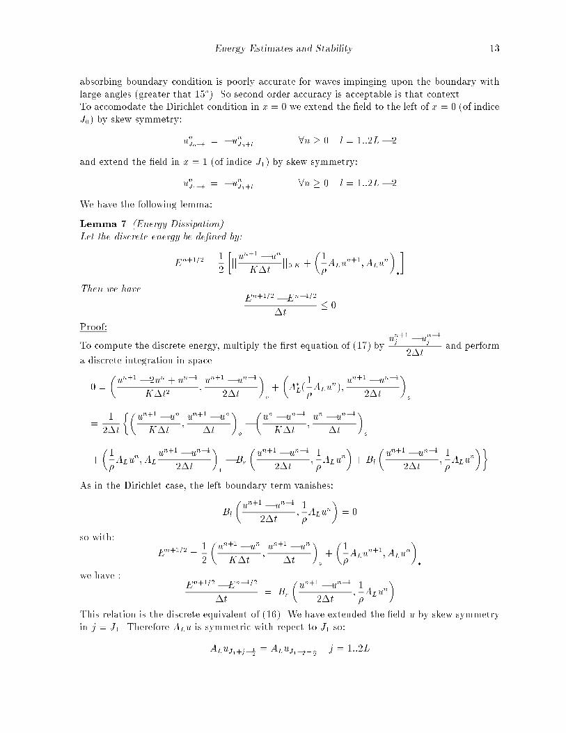
Energy Estimates and Stability 13
absorbing boundary condition is poorly accurate for waves impinging upon the boundary with
large angles (greater that 15o). So second order accuracy is acceptable is that context.
To accomodate the Dirichlet condition in x = 0 we extend the �eld to the left of x = 0 (of indice
J0) by skew symmetry:
unJ0�l = �unJ0+l 8n � 0 l = 1::2L� 2
and extend the �eld in x = 1 (of indice J1) by skew symmetry:
unJ1�l = �unJ1+l 8n � 0 l = 1::2L� 2
We have the following lemma:
Lemma 7 (Energy Dissipation)
Let the discrete energy be de�ned by:
En+1=2 =1
2
�jju
n+1 � un
K�tjj0;K +
�1
�ALu
n+1; ALun
��
�
Then we haveEn+1=2� En�1=2
�t� 0
Proof:
To compute the discrete energy, multiply the �rst equation of (17) byun+1j � un�1j
2�tand perform
a discrete integration in space.
0 =
�un+1 � 2un + un�1
K�t2;un+1 � un�1
2�t
�o
+
�A�L(
1
�ALu
n);un+1 � un�1
2�t
�o
=1
2�t
��un+1 � un
K�t;un+1 � un
�t
�o
��un � un�1
K�t;un � un�1
�t
�o
+
�1
�ALu
n; AL
un+1 � un�1
2�t
��
� Br
�un+1 � un�1
2�t;1
�ALu
n
�+ Bl
�un+1 � un�1
2�t;1
�ALu
n
��
As in the Dirichlet case, the left boundary term vanishes:
Bl
�un+1 � un�1
2�t;1
�ALu
n
�= 0
so with:
En+1=2 =1
2
�un+1 � un
K�t;un+1 � un
�t
�o
+
�1
�ALu
n+1; ALun
��
we have :En+1=2� En�1=2
�t= Br
�un+1 � un�1
2�t;1
�ALu
n
�
This relation is the discrete equivalent of (16). We have extended the �eld u by skew symmetry
in j = J1. Therefore ALu is symmetric with repect to J1 so:
ALuJ1+j�12= ALuJ1�j+ 1
2j = 1::2L
14 Alain Sei
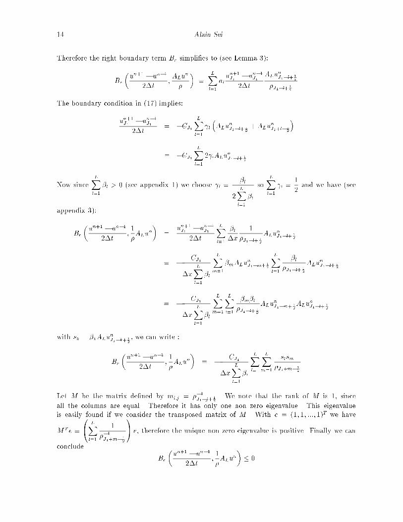
Therefore the right boundary term Br simpli�es to (see Lemma 3):
Br
�un+1 � un�1
2�t;ALu
n
�
�=
LXl=1
alun+1J1
� un�1J1
2�t
ALunJ1�l+
12
�J1�l+ 12
The boundary condition in (17) implies:
un+1J1� un�1J1
2�t= �CJ1
LXl=1
l
�ALu
nJ1�l+
12+ALu
nJ1+l�
12
�
= �CJ1
LXl=1
2 lALunJ1�l+
12
Now sinceLXl=1
�l > 0 (see appendix 1) we choose l =�l
2LXl=1
�l
soLXl=1
l =1
2and we have (see
appendix 3):
Br
�un+1 � un�1
2�t;1
�ALu
n
�=
un+1J1� un�1J1
2�t
LXl=1
�l
�x
1
�J1�l+ 12
ALunJ1�l+
12
= � CJ1
�xLXl=1
�l
LXm=1
�mALunJ1�m+
12
LXl=1
�l
�J1�l+ 12
ALunJ1�l+
12
= � CJ1
�xLXl=1
�l
LXm=1
LXl=1
�m�l
�J1�l+ 12
ALunJ1�m+
12ALu
nJ1�l+
12
with sk = �kALunJ1�k+
12, we can write :
Br
�un+1 � un�1
2�t;1
�ALu
n
�= � CJ1
�xLXl=1
�l
LXl=1
LXm=1
slsm
�J1+m� 12
Let M be the matrix de�ned by mi;j = ��1J1�j+
12. We note that the rank of M is 1, since
all the columns are equal. Therefore it has only one non zero eigenvalue. This eigenvalue
is easily found if we consider the transposed matrix of M . With e = (1; 1; :::; 1)T we have
MTe =
0@ LX
l=1
1
��1J1+m�
12
1A e, therefore the unique non zero eigenvalue is positive. Finally we can
conclude
Br
�un+1 � un�1
2�t;1
�ALu
n
�� 0
Energy Estimates and Stability 15
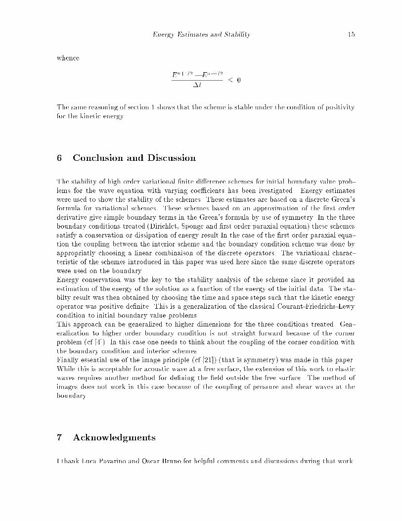
whence
En+1=2 �En�1=2
�t� 0
The same reasoning of section 1 shows that the scheme is stable under the condition of positivity
for the kinetic energy.
6 Conclusion and Discussion
The stability of high order variational �nite di�erence schemes for initial boundary value prob-
lems for the wave equation with varying coe�cients has been ivestigated. Energy estimates
were used to show the stability of the schemes. These estimates are based on a discrete Green's
formula for variational schemes. These schemes based on an approximation of the �rst order
derivative give simple boundary terms in the Green's formula by use of symmetry. In the three
boundary conditions treated (Dirichlet, Sponge and �rst order paraxial equation) these schemes
satisfy a conservation or dissipation of energy result.In the case of the �rst order paraxial equa-
tion the coupling between the interior scheme and the boundary condition scheme was done by
appropriatly choosing a linear combinaison of the discrete operators. The variational charac-
teristic of the schemes introduced in this paper was used here since the same discrete operators
were used on the boundary.
Energy conservation was the key to the stability analysis of the scheme since it provided an
estimation of the energy of the solution as a function of the energy of the initial data. The sta-
bilty result was then obtained by choosing the time and space steps such that the kinetic energy
operator was positive de�nite. This is a generalization of the classical Courant-Friedrichs-Lewy
condition to initial boundary value problems.
This approach can be generalized to higher dimensions for the three conditions treated. Gen-
eralization to higher order boundary condition is not straight forward because of the corner
problem (cf [4]). In this case one needs to think about the coupling of the corner condition with
the boundary condition and interior schemes.
Finally essential use of the image principle (cf [21]) (that is symmetry) was made in this paper.
While this is acceptable for acoustic wave at a free surface, the extension of this work to elastic
waves requires another method for de�ning the �eld outside the free surface. The method of
images does not work in this case because of the coupling of pressure and shear waves at the
boundary.
7 Acknowledgments
I thank Luca Pavarino and Oscar Bruno for helpful comments and discussions during that work.
16 Alain Sei
8 Appendix
8.1 Appendix 1
For the scheme to be consistent �l verifyLXl=1
�l
2l � 1= 1 and to approximate the �rst derivative
to order 2LLXl=1
(2l� 1)2p�1�l = 0 p = 1; ::; L
Solving this linear system in �l gives:
�l =(�1)l+1
2l� 1
Ym6=l
(2m� 1)2
jYm6=l
(2m� 1)2 � (2l� 1)2 j
8.2 Appendix 2
We want to prove that the semi norm de�ned on H1L is a norm. We only need to prove that
jjujjH1L= 0 =) u = 0. We have
jjujjH1L= 0 () jjALujj� = 0
()J�1Xj=0
(ALu)2j+1=2 = 0
=)LXl=1
�l(uj+l � uj�l+1) = 0 j = 0; ::; J � 1
We can write this linear system of equations in matrix form. With the vector ~U and the matrix
B de�ned by~UT = (u1�L; :::; u1; :::; uJ; :::; uJ�L+1)
B =
0BBBBBBBBBBBB@
��L � �L�1 � � � �L�1 �L 0 � � � 0
0 � �L � �L�1 � � � �L�1 �L 0 � � � 0:
:
:
:
0 � � � 0 � �L � �L�1 � � � �L�1 �L
1CCCCCCCCCCCCA
we can write the previous equations as
B:~U = 0
B is a J + 2L� 1 by J matrix. If we consider ~U 0 composed of the J �rst components of ~U and
the matrix B0 composed of the �rst J line of B, we �nd ~U 0 solution of
B0: ~U 0 = 0
Energy Estimates and Stability 17
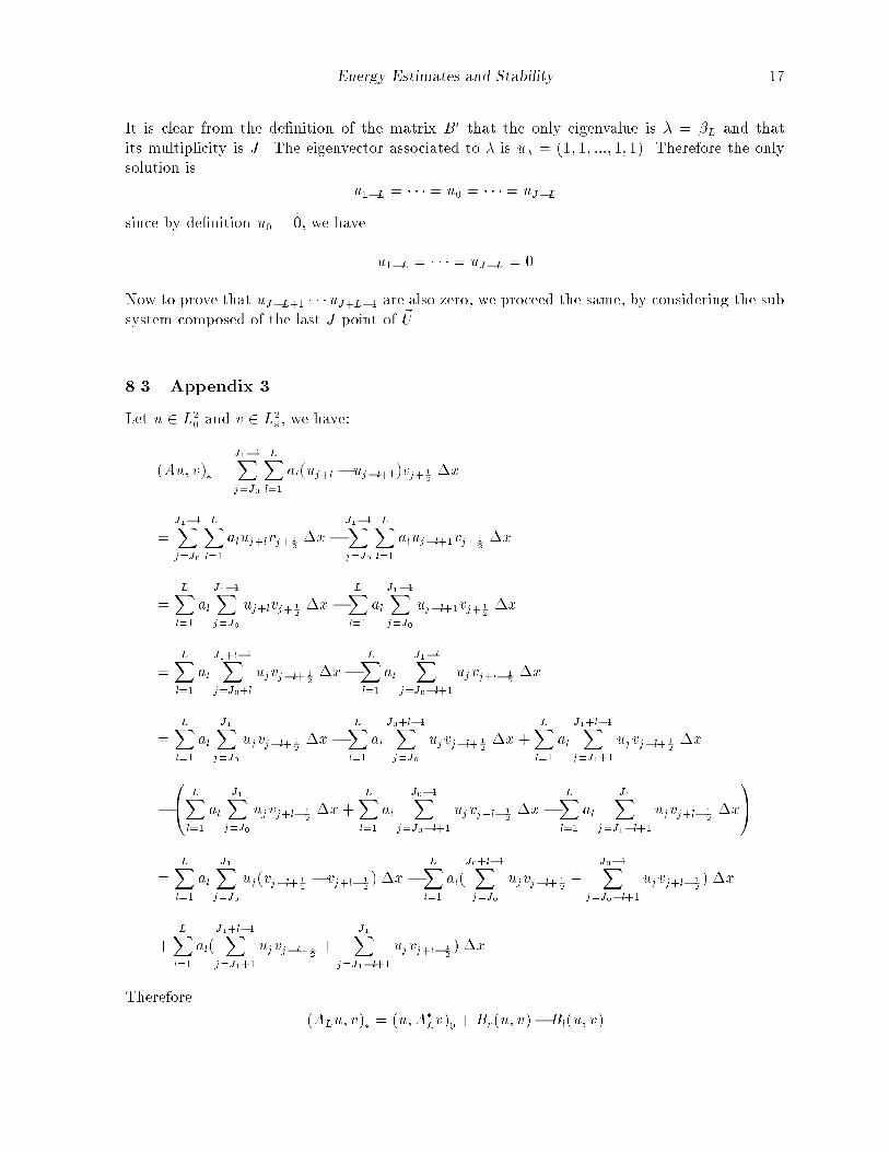
It is clear from the de�nition of the matrix B0 that the only eigenvalue is � = �L and that
its multiplicity is J . The eigenvector associated to � is u� = (1; 1; :::; 1; 1). Therefore the only
solution is
u1�L = � � �= u0 = � � �= uJ�L
since by de�nition u0 = 0, we have
u1�L = � � � = uJ�L = 0
Now to prove that uJ�L+1 � � �uJ+L�1 are also zero, we proceed the same, by considering the sub
system composed of the last J point of ~U .
8.3 Appendix 3
Let u 2 L20 and v 2 L2�, we have:
(Au; v)� =J1�1Xj=J0
LXl=1
al(uj+l � uj�l+1)vj+ 12�x
=J1�1Xj=J0
LXl=1
aluj+lvj+ 12�x�
J1�1Xj=J0
LXl=1
aluj�l+1vj+ 12�x
=LXl=1
al
J1�1Xj=J0
uj+lvj+ 12�x�
LXl=1
al
J1�1Xj=J0
uj�l+1vj+ 12�x
=LXl=1
al
J1+l�1Xj=J0+l
ujvj�l+ 12�x�
LXl=1
al
J1�lXj=J0�l+1
ujvj+l� 12�x
=LXl=1
al
J1Xj=J0
ujvj�l+ 12�x�
LXl=1
al
J0+l�1Xj=J0
ujvj�l+ 12�x+
LXl=1
al
J1+l�1Xj=J1+1
ujvj�l+ 12�x
�0@ LX
l=1
al
J1Xj=J0
ujvj+l� 12�x+
LXl=1
al
J0�1Xj=J0�l+1
ujvj+l� 12�x�
LXl=1
al
J1Xj=J1�l+1
ujvj+l� 12�x
1A
=LXl=1
al
J1Xj=J0
uj(vj�l+ 12� vj+l� 1
2) �x�
LXl=1
al(J0+l�1Xj=J0
ujvj�l+ 12+
J0�1Xj=J0�l+1
ujvj+l� 12) �x
+LXl=1
al(J1+l�1Xj=J1+1
ujvj�l+ 12+
J1Xj=J1�l+1
ujvj+l� 12) �x
Therefore
(ALu; v)� = (u;A�Lv)0 +Br(u; v)� Bl(u; v)
18 Alain Sei
with
Br(u; v) =LXl=1
al(J1+l�1Xj=J1+1
ujvj�l+ 12+
J1Xj=J1�l+1
ujvj+l� 12) �x
Bl(u; v) =LXl=1
al(J0+l�1Xj=J0
ujvj�l+ 12+
J0�1Xj=J0�l+1
ujvj+l� 12) �x
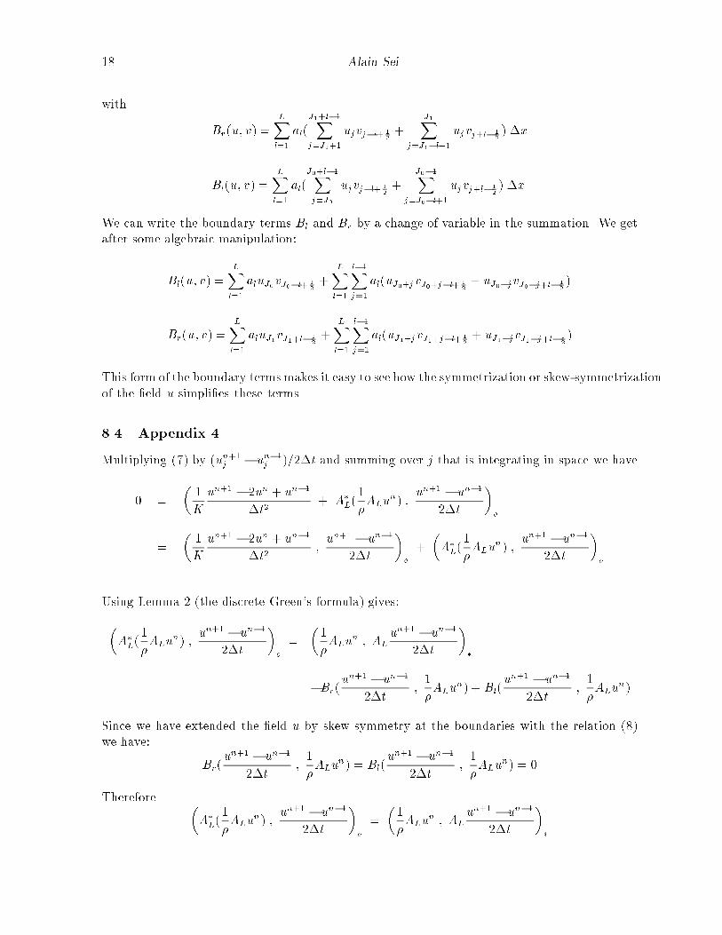
We can write the boundary terms Bl and Br by a change of variable in the summation. We get
after some algebraic manipulation:
Bl(u; v) =LXl=1
aluJ0vJ0�l+ 12+
LXl=1
l�1Xj=1
al(uJ0+jvJ0+j�l+ 12+ uJ0�jvJ0�j+l� 1
2)
Br(u; v) =LXl=1
aluJ1vJ1+l� 12+
LXl=1
l�1Xj=1
al(uJ1+jvJ1+j�l+ 12+ uJ1�jvJ1�j+l� 1
2)
This form of the boundary termsmakes it easy to see how the symmetrization or skew-symmetrization
of the �eld u simpli�es these terms.
8.4 Appendix 4
Multiplying (7) by (un+1j � un�1j )=2�t and summing over j that is integrating in space we have
0 =
�1
K
un+1 � 2un + un�1
�t2+ A�L(
1
�ALu
n) ;un+1 � un�1
2�t
�o
=
�1
K
un+1 � 2un + un�1
�t2;un+1 � un�1
2�t
�o
+
�A�L(
1
�ALu
n) ;un+1 � un�1
2�t
�o
Using Lemma 2 (the discrete Green's formula) gives:
�A�L(
1
�ALu
n) ;un+1 � un�1
2�t
�o
=
�1
�ALu
n ; AL
un+1 � un�1
2�t
��
�Br(un+1 � un�1
2�t;1
�ALu
n) +Bl(un+1 � un�1
2�t;1
�ALu
n)
Since we have extended the �eld u by skew symmetry at the boundaries with the relation (8)
we have:
Br(un+1 � un�1
2�t;1
�ALu
n) = Bl(un+1 � un�1
2�t;1
�ALu
n) = 0
Therefore �A�L(
1
�ALu
n) ;un+1 � un�1
2�t
�o
=
�1
�ALu
n ; AL
un+1 � un�1
2�t
��
Energy Estimates and Stability 19
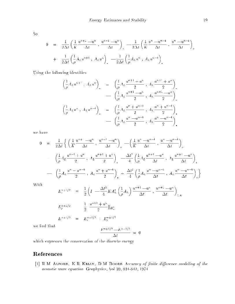
So
0 =1
2�t
�1
K
un+1 � un
�t;un+1 � un
�t
�o
� 1
2�t
�1
K
un � un�1
�t;un � un�1
�t
�o
+1
2�t
�1
�ALu
n+1 ; ALun
��
� 1
2�t
�1
�ALu
n ; ALun�1
��
Using the following identities
�1
�ALu
n+1 ; ALun
��
=
�1
�AL
un+1 + un
2; AL
un+1 + un
2
��
��1
�AL
un+1 � un
2; AL
un+1 � un
2
���
1
�ALu
n ; ALun�1
��
=
�1
�AL
un + un�1
2; AL
un + un�1
2
��
��1
�AL
un � un�1
2; AL
un � un�1
2
��
we have
0 =1
2�t
� �1
K
un+1 � un
�t;un+1 � un
�t
�o
��1
K
un � un�1
�t;un � un�1
�t
�o
+
�1
�AL
un+1 + un
2; AL
un+1 + un
2
��
� �t2
4
�1
�AL
un+1 � un
�t; AL
un+1 � un
�t
��
��1
�AL
un + un�1
2; AL
un + un�1
2
��
+�t2
4
�1
�AL
un � un�1
�t; AL
un � un�1
�t
��
�
With
En+1=2c =
1
2
�I � �t2
4KA�L
�1
�AL
�un+1 � un
�t;un+1 � un
�t
�0;K
En+1=2p =
1
2jju
n+1 + un
2jjH1
L
En+1=2 = En+1=2c + En+1=2
p
we �nd thatEn+1=2�En+1=2
�t= 0
which expresses the conservation of the discrete energy.
References
[1] R.M Alford, K.R Kelly, D.M Boore Accuracy of �nite di�erence modeling of the
acoustic wave equation. Geophysics, Vol 39, 834-842, 1974.
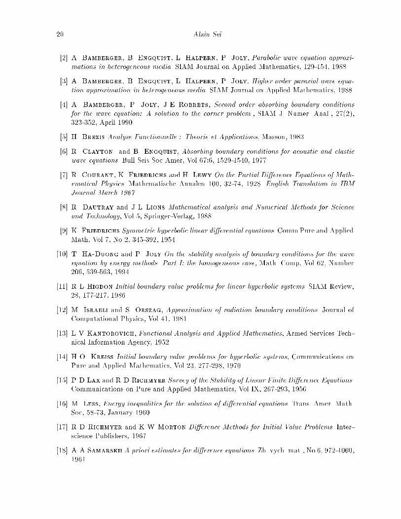
20 Alain Sei
[2] A. Bamberger, B. Engquist, L. Halpern, P. Joly, Parabolic wave equation approxi-
mations in heterogeneous media. SIAM Journal on Applied Mathematics, 129-154, 1988.
[3] A. Bamberger, B. Engquist, L. Halpern, P. Joly, Higher order paraxial wave equa-
tion approximation in heterogeneous media. SIAM Journal on Applied Mathematics, 1988.
[4] A. Bamberger, P. Joly, J.E Robrets, Second order absorbing boundary conditions
for the wave equation: A solution to the corner problem., SIAM J. Numer. Anal., 27(2),
323-352, April 1990.
[5] H. Brezis Analyse Functionnelle : Theorie et Applications, Masson, 1983.
[6] R. Clayton and B. Engquist, Absorbing boundary conditions for acoustic and elastic
wave equations. Bull Seis Soc Amer, Vol 67:6, 1529-1540, 1977.
[7] R. Courant, K. Friedrichs and H. Lewy On the Partial Di�erence Equations of Math-
ematical Physics. Mathematische Annalen 100, 32-74, 1928. English Translation in IBM
Journal March 1967.
[8] R. Dautray and J.L Lions Mathematical analysis and Numerical Methods for Science
and Technology, Vol 5, Springer-Verlag, 1988.
[9] K. Friedrichs Symmetric hyperbolic linear di�erential equations. Comm Pure and Applied
Math, Vol 7, No 2, 345-392, 1954.
[10] T. Ha-Duong and P. Joly On the stability analysis of boundary conditions for the wave
equation by energy methods. Part I: the homogeneous case, Math. Comp, Vol 62, Number
206, 539-563, 1994.
[11] R.L Higdon Initial boundary value problems for linear hyperbolic systems. SIAM Review,
28, 177-217, 1986.
[12] M. Israeli and S. Orszag, Approximation of radiation boundary conditions. Journal of
Computational Physics, Vol 41, 1981.
[13] L.V Kantorovich, Functional Analysis and Applied Mathematics, Armed Services Tech-
nical Information Agency, 1952.
[14] H.O. Kreiss Initial boundary value problems for hyperbolic systems, Communications on
Pure and Applied Mathematics, Vol 23, 277-298, 1970.
[15] P.D Lax and R.D Richmyer Survey of the Stability of Linear Finite Di�erence Equations.
Communications on Pure and Applied Mathematics, Vol IX, 267-293, 1956.
[16] M. Less, Energy inequalities for the solution of di�erential equations. Trans. Amer. Math.
Soc, 58-73, January 1960.
[17] R.D Richmyer and K.W Morton Di�erence Methods for Initial Value Problems. Inter-
science Publishers, 1967.
[18] A.A Samarskii A priori estimates for di�erence equations. Zh. vych. mat., No 6, 972-1000,
1961.
Energy Estimates and Stability 21
[19] A. Sei, A Family of schemes for the computation of elastic waves. SIAM Journal on Sci-
enti�c Computing, Vol 16, Number 4, pp 898-916.
[20] R. Vichnevetski and J. Bowles, Fourier analysis of numerical approximations of hy-
perbolic equations, Philadelphia, SIAM, 1982.
[21] A.N Tikhonov andA.A SamarskiiPartial di�erential equations of mathematical physics.
San Francisco. Holden-Day, 1964.


![Alain Bashung - Alain Bashung [PVC Book]](https://img.dokumen.tips/doc/110x75/55cf868e550346484b98cd83/alain-bashung-alain-bashung-pvc-book.jpg)